Estimating $\chi_{\mathrm{top}}$ Lattice Artifacts from Flowed SU(2) Calorons

Abstract

Lattice computations of the high-temperature topological susceptibility of QCD receive lattice-spacing corrections and suffer from systematics arising from the type and depth of gradient flow. We study the lattice spacing corrections to $\chi_{\mathrm{top}}$ semi-analytically by exploring the behavior of discretized Harrington-Shepard calorons under the action of different forms of gradient flow. From our study we conclude that $N_{\tau}=6$ is definitely too small of a time extent to study the theory at temperatures of order $4~{}T_{\mathrm{c}}$ and we explore how the amount of gradient flow influences the continuum extrapolation.

1 Introduction

Quantum Chromodynamics fields generically contain topological structure, which may play a role in some low-energy phenomenology and have been treated extensively in the literature Schafer:1996wv . This paper shall put the focus on topology at high temperatures $T\gg T_{\mathrm{c}}$ the (crossover) temperature. At these temperatures, the topological susceptibility – the mean-squared $Q$-value per unit 4-volume – is small, but it nevertheless plays a crucial role in the cosmological physics of the QCD axion Peccei:1977ur ; Weinberg:1977ma ; Wilczek:1977pj ; Preskill:1982cy ; Abbott:1982af ; Dine:1982ah , should it exist. In this case, besides the now rather well-determined value of the topological susceptibility in vacuum diCortona:2015ldu , we also need the topological susceptibility in the temperature range $3~{}T_{\mathrm{c}}$ – $7~{}T_{\mathrm{c}}$ Klaer:2017ond ; Moore:2017ond , since this is the temperature range where a cosmological axion density would be established. The exploration of topological susceptibility at high temperatures within QCD has recently become the topic of intense investigation Berkowitz:2015aua ; Borsanyi:2015cka ; Petreczky:2016vrs ; Taniguchi:2016tjc ; Burger:2017xkz ; Frison:2016vuc ; Borsanyi:2016ksw ; Jahn:2018dke . (For a recent review of the axion see Ref. Irastorza:2018dyq .)

At low temperatures, topology is dominated by long range physics where the coupling is strong. In this regime, we have little rigorous theoretical guidance for the form of the configurations which predominantly contribute to the topological susceptibility. On the other hand, at high temperatures the coupling is weak and Gross, Pisarski, and Yaffe Gross:1980br demonstrated that the dominant configurations are expected to be calorons (periodic instantons) with radius $\rho$ of order of half the inverse temperature. Smaller objects are suppressed by the smaller coupling at short distances, and larger objects are suppressed by their interaction with thermal fluctuations. In general, at high temperatures, topological objects are rare and can be treated singly (dilute instanton gas).

At the temperature range relevant for axion cosmology, topological objects should be dilute, but corrections to perturbation theory may be large. In particular, the calculation of the thermal corrections to the caloron action is not secure due to the infrared issues of thermal fluctuations which exist even at weak coupling in gauge theories Linde:1980ts ; diCortona:2015ldu . Those can influence the environment of the caloron and change the exact coefficient of the $\exp(-\rho^{2}T^{2})$ suppression of large calorons. Therefore a nonperturbative lattice treatment would be very valuable. But this brings with it some complications. Strictly speaking, there is no perfectly clean and unambiguous definition for topology on the lattice. After all, on a compact space without boundary, topology partitions the space of smooth continuum configurations into path-disconnected subspaces with different integer $Q$ values. But the space of lattice configurations is $[\mathrm{SU}(N)]^{N_{\ell}}$ (with $N_{\ell}$ the number of lattice links), which is path connected, precluding a continuous and integer definition of $Q$. This problem has long been appreciated; Lüscher showed that topology becomes well defined if we restrict to sufficiently “smooth” lattice configurations, in the sense that all plaquettes are suitably close to the identity Luscher:1981zq . That means that the failure for a perfectly clean definition of topology on the lattice lies with certain very non-smooth configurations, termed “dislocations.”

A modern tool for studying topology on the lattice is the integration of a lattice discretized version of $Q$ after the lattice fields have been subjected to gradient flow Narayanan:2006rf ; Luscher:2009eq . This definition has its roots in older studies employing cooling Berg:1981nw ; deForcrand:1997esx ; GarciaPerez:1998ru ; GarciaPerez:1999hs , with gradient flow representing a better-controlled and better-understood form of gauge-link cooling. With gradient flow, a well-defined parameter $t$ controls the extent of smearing applied. Gradient flow tends to eliminate dislocations Teper:1985rb , but since there is no clean distinction between dislocations and small-but-physical instantons, it may also destroy the smallest instantons which we want to keep. This issue is addressed phenomenologically in most lattice studies that attempt a calculation of the topological susceptibility, but we are surprised by the absence of a more systematic study, which might help in understanding how wide the flow time window actually is, and how large we should expect the lattice artifacts in the topological susceptibility to be. In other words, it would be useful to get a better analytical understanding of how lattice spacing and flow-depth effects may influence the determined topological susceptibility.

In this paper we shall explore this issue by studying exactly how much gradient flow destroys exactly what size of Harrington-Shepard calorons Harrington:1978ve . This requires a lattice implementation of the caloron, which we supply. We also explore different implementations of gradient flow: a.) Wilson flow Luscher:2009eq , b.) a recently proposed $\mathcal{O}\mathopen{}\mathclose{{}\left(a^{2}}\right)$-improved flow dubbed Zeuthen flow Ramos:2015baa , and c.) an “overimproved” flow in which we force the $a^{2}$ errors in the flow action to have the opposite sign as in Wilson flow. We are hardly the first to implement discretized topological configurations on the lattice Pugh:1989ek ; Bruckmann:2004nu ; Bruckmann:2004zy or to consider topology after cooling deForcrand:1995qq ; deForcrand:1995bq ; deForcrand:1997esx ; GarciaPerez:1998ru ; GarciaPerez:1999hs . But our emphasis is a little different; we want to understand and control what size of dislocation/caloron survives what amount of flow, and what impact this may have on the determination of the topological susceptibility at finite lattice spacing and on the corresponding extrapolation to the continuum limit.

A natural objection to our study is that, in the temperature range of relevance, the coupling is still quite large. Therefore, the actual topological objects from the lattice will not be clean calorons, but will have large fluctuations. Nonetheless, gradient flow will drive any topological object towards a caloron solution in a much smaller amount of flow time than it takes for the object to disappear, since the caloron is a stationary point of the action up to $a^{2}$ corrections. Therefore the actual topological objects’ flow trajectories should be very similar to those for calorons. (In fact, in the continuum, we could even define the size of a topological object to be the size of the caloron it approaches under gradient flow.) Therefore our study can still shed light on how much flow removes what size of topological object. Combining this with an estimate, based on Gross Pisarski and Yaffe’s work, for the size distribution of calorons, can illuminate what flow depths affect the topological objects we want to keep, and what lattice spacings may be too coarse to distinguish between dislocations and physically relevant topological objects.

The paper is structured as follows: In Sec. 2 we collect our definitions and define our topology configurations at finite temperature. Section 3 then introduces the different flows and flow actions. In Sec. 4 we compute $\rho_{\mathrm{crit}}(t)$ which indicate the value of the radius of a caloron that barely survived the amount of flow time $t$. These curves are further used in Sec. 5 to estimate how lattice spacing systematics interfere with flow effects in the approach to the continuum. An example study at $T=4~{}T_{\mathrm{c}}$ is used. Our conclusions can then be found in Sec. 6.

2 Caloron discretization with $Q=1$

The Harrington-Shepard caloron Harrington:1978ve can be understood as the finite temperature generalization of the BPST instanton tHooft:1976rip . The most straightforward way of constructing the solution is to recognize that one has to take into account the infinite time copies that arise due to the compactification of the Euclidean time direction whose inverse length plays the role of temperature ($\beta\equiv T^{-1}$). Following Jackiw:1976fs we consider a superpotential of the form

$$\Phi_{\mathrm{HS}}(x) =1+\sum_{k\in\mathds{Z}}\frac{\rho^{2}}{\mathopen{}\mathclose{{}\left(x-z_{k}}\right)^{2}}$$

$$=1+\frac{\pi\rho^{2}\sinh\frac{2\pi\mathopen{}\mathclose{{}\left|\vec{x}-\vec{z}}\right|}{\beta}}{\beta\mathopen{}\mathclose{{}\left|\vec{x}-\vec{z}}\right|\mathopen{}\mathclose{{}\left(\cosh\frac{2\pi\mathopen{}\mathclose{{}\left|\vec{x}-\vec{z}}\right|}{\beta}-\cos\frac{2\pi\mathopen{}\mathclose{{}\left(x_{0}-z_{0}}\right)}{\beta}}\right)}$$ (1)

with $z_{k}=\mathopen{}\mathclose{{}\left(z_{0}+k\beta,\vec{z}}\right)$ and $\rho$ having length-units and playing the role of the caloron radius. Concentrating on SU(2) calorons, the gauge field continuum form is obtained via

$$A_{\mu}^{a}(x)=\eta_{a\mu\nu}\partial_{\nu}\ln\Phi_{\mathrm{HS}}(x),$$ (2)

where $\eta_{a\mu\nu}=\epsilon_{0a\mu\nu}+\delta_{a\mu}\delta_{\nu 0}-\delta_{a\nu}\delta_{\mu 0}$ is the ’t Hooft symbol (equivalently for $\bar{\eta}_{a\mu\nu}$ the sign of the last two terms is reversed and one obtains an anti-instanton with $Q=-1$) tHooft:1976rip . The self-duality condition $F_{\mu\nu}=\frac{1}{2}\epsilon_{\mu\nu\rho\sigma}F_{\rho\sigma}$, implies that a valid solution for $A_{\mu}(x)$ is obtained if $\Phi_{\mathrm{HS}}(x)$ obeys the Poisson equation $\square\Phi_{\mathrm{HS}}=0$.

It is a tedious but straightforward exercise to check that indeed this gauge field yields $Q=1$ and $S=8\pi^{2}$. Notice that it is given in singular gauge, meaning that there is a singularity at the center of the caloron when $x=z$ . Next, we use the path-ordered exponential map to obtain the expression for the lattice links as

$$U_{\mu}(x)=\mathcal{P}\exp\mathopen{}\mathclose{{}\left[a\int_{0}^{1}\mathrm{d}t\ A_{\mu}\mathopen{}\mathclose{{}\left(\Gamma_{\mu}(x,t)}\right)}\right],$$ (3)

where $\Gamma_{\mu}(x,t)=x+ta\hat{\mu}$ is an appropriate parameterization for the corresponding path connecting the two neighboring lattice sites $x$ and $x+a\hat{\mu}$ with $t\in[0,1]$ (no summation over $\mu$ is implied in Eq. (3)).

In the case of an instanton (without periodic images), $A_{\mu}$ commutes everywhere along a link, but this turns out not to be true for the caloron. In order to compute the links we rewrite Eq. (3) as a product of $n$ shorter links,

$$U_{\mu}(x)=\lim_{n\to\infty}\>\mathcal{P}\prod_{k=1}^{n}\exp\mathopen{}\mathclose{{}\left[\frac{a}{n}A_{\mu}\mathopen{}\mathclose{{}\left(\Gamma_{\mu}\mathopen{}\mathclose{{}\left(x,\frac{2k-1}{2n}}\right)}\right)}\right],$$ (4)

where in practice we use $n\sim 40$ rather than taking the strict $n\to\infty$ limit. Periodicity is imposed in all four dimensions, and while boundary effects are absent in the time direction, our lattice field will have a discontinuity at the spatial edges of the box. We ameliorate this problem with gradient flow confined to the boundary region as described in App. A.

Finally the embedding into an SU(3) background is trivial since a particular lattice gauge exists in which the links take the following form:

$$U^{\mathrm{SU(3)}}_{\mu}=\mathopen{}\mathclose{{}\left(\begin{array}[]{c|c}U^{\mathrm{SU(2)}}_{\mu}&\begin{matrix}0\\ 0\end{matrix}\\ \hline\cr\begin{matrix}0&0\end{matrix}&1\\ \end{array}}\right).$$ (5)

Therefore we are effectively considering SU(2) configurations in this paper. This makes our study less general than Ref. Bruckmann:2004nu , who also consider calorons in the background of nontrivial holonomy. Note, however, that if we are primarily interested in high temperatures, nontrivial holonomy is not likely to be relevant, since fluctuations create an effective potential for the Polyakov loop which favors trivial holonomy Gross:1980br .

3 Gradient Flows

Gradient flow and its discretized version on the lattice Narayanan:2006rf ; Luscher:2009eq ; Luscher:2010iy ; Luscher:2010we ; Luscher:2011bx ; Luscher:2013cpa have become an essential tool to reduce UV fluctuations. In the continuum it defines a mapping of the gauge fields $A_{\mu}(x)$ to smeared gauge fields $B_{\mu}(x,t)$, where $t$ is the so-called flow time, via the flow equation

$$\partial_{t}B_{\mu}=D_{\nu}F_{\nu\mu},\qquad B_{\mu}(x,0)=A_{\mu}(x).$$ (6)

The right-hand side of this differential equation is nothing but the classical equations of motion. Consequently, it will drive the gauge field along the trajectory of steepest descent minimizing the action along the way. On the lattice the simplest form reads

$$a^{2}\partial_{t}V_{\mu}(x,t)=-g_{0}^{2}\partial_{x,\mu}S_{\mathrm{W}}[V]V_{\mu}(x,t),$$ (7)

where $V_{\mu}(x,t)$ is the flowed gauge field with initial condition $V_{\mu}(x,0)=U_{\mu}(x)$ and $S_{\mathrm{W}}$ denotes the Wilson plaquette action. The Lie-algebra valued derivative of a general function of the link variables $f(U_{\mu})$ is given by

$$\partial_{x,\mu}^{a}f(U_{\mu}(x))=\mathopen{}\mathclose{{}\left.T^{a}\frac{\mathrm{d}}{\mathrm{d}s}f\mathopen{}\mathclose{{}\left(\mathrm{e}^{sT^{a}}U_{\mu}(x)}\right)}\right|_{s=0}.$$ (8)

Recently, an $\mathcal{O}\mathopen{}\mathclose{{}\left(a^{2}}\right)$ improved version of the flow equation was developed in Ref. Ramos:2015baa . The so-called Zeuthen flow equation reads

$$a^{2}\partial_{t}V_{\mu}(x,t)=-g_{0}^{2}\mathopen{}\mathclose{{}\left(1+\frac{a^{2}}{12}\nabla_{\mu}^{\ast}\nabla_{\mu}}\right)\partial_{x,\mu}S_{\mathrm{Sym}}[V]V_{\mu}(x,t),$$ (9)

where $S_{\mathrm{Sym}}$ is the tree-level improved Symanzik action Luscher:1984xn and the discretized adjoint covariant derivative is given by

$$\begin{split}a\nabla_{\mu}f(x)&=U_{\mu}(x)f(x+a\hat{\mu})U_{\mu}^{\dagger}(x)-f(x),\\ a\nabla_{\mu}^{\ast}f(x)&=f(x)-U_{\mu}^{\dagger}(x-a\hat{\mu})f(x-a\hat{\mu})U_{\mu}(x-a\hat{\mu}).\end{split}$$ (10)

The unexpected additional factor $(1+a^{2}\nabla_{\mu}^{\ast}\nabla^{\mu}/12)$ can be understood as follows. We know that improvement requires replacing square plaquettes with a linear combination of squares and rectangles. The Symanzik action does this in the four spacetime directions. The added term does it in the flow-time direction. Ref. Ramos:2015baa have proven that this gives a (tree-level) $\mathcal{O}\mathopen{}\mathclose{{}\left(a^{2}}\right)$ improvement of the flow equation. In addition to these two we investigate a flow equation with an overimproved action (precise definitions of these actions are given in Subsec. 4.1)

$$a^{2}\partial_{t}V_{\mu}(x,t)=-g_{0}^{2}\mathopen{}\mathclose{{}\left(\partial_{x,\mu}S_{\mathrm{OI}}[V]}\right)V_{\mu}(x,t).$$ (11)

We expect this flow equation to allow for stable topological solutions under flow. Notice that the flow equations Eqs. (7), (9), and (11) do not depend on $g^{2}_{0}$ at all since the actions themselves carry such a factor, too. We therefore omit $g^{2}_{0}$ factors when not relevant for the discussion.

The goal is to study the effect of Eqs. (7), (9), and (11) on our constructed clean topological configurations to learn about how their topological properties are changed. This can represent interesting information to better control systematic errors when performing lattice calculations of topological observables with the help of flow.

4 Lattice Caloron Properties

Mainly we will focus on the measurement of the topological charge $Q$ and the action $S$ which in the continuum take the values $Q=1$ and $S=8\pi^{2}$, respectively. Deviations from these numbers occur on a finite lattice due to cutoff and boundary effects. We will try to disentangle those to more deeply understand the effect of flow.

4.1 Actions

Throughout this work we consider Lüscher-Weisz actions of the form Luscher:1984xn ; openQCD (omitting $g^{2}_{0}$ factors)

$$S(c_{0},c_{1}) =2\mathopen{}\mathclose{{}\left(c_{0}\sum_{x}\mathrm{Re}\mathrm{tr}\mathopen{}\mathclose{{}\left(\mathds{1}-U_{\mathrm{P}}(x)_{(1,1)}}\right)}\right.$$

$$+\mathopen{}\mathclose{{}\left.c_{1}\sum_{x}\mathrm{Re}\mathrm{tr}\mathopen{}\mathclose{{}\left(\mathds{1}-U_{\mathrm{R}}(x)_{(2,1)}}\right)}\right),$$ (12)

where $U_{\mathrm{P}}(x)_{(1,1)}$ denotes the simple closed plaquette and $U_{\mathrm{R}}(x)_{(2,1)}$ are $2\times 1$ (and $1\times 2$) rectangles where both loop orientations are taken into account by the $\mathrm{Re}\mathrm{tr}$ operation. A correct normalization requires $c_{0}+8c_{1}=1$. The three actions going into the three different flow equations can be summarized as follows:

$$S\mathopen{}\mathclose{{}\left(1,0}\right) =S_{\mathrm{W}}\qquad$$ (Wilson),

$$S\mathopen{}\mathclose{{}\left(5/3,-1/12}\right) =S_{\mathrm{Sym}}\qquad$$ (Symanzik), (13)

$$S\mathopen{}\mathclose{{}\left(7/3,-1/6}\right) =S_{\mathrm{OI}}\qquad$$ (Overimproved).

Fig. 1 explores how each action varies as a function of the caloron size $\rho T$, on a lattice with $N_{\tau}=8$ and an aspect ratio of 6. We find that all actions start small and are suppressed until about $\rho=1.6a$, which is $\rho T=0.2$ for this $N_{\tau}$ value. A rapid rise towards the expected value of $8\pi^{2}$ is then observed, followed eventually by a rise above $8\pi^{2}$. These two features – the rapid rise from zero towards $8\pi^{2}$, and the eventual rise above this value – arise from different artifacts. The former is a lattice spacing artifact, which we now explore. We overlay each curve with an estimate based on a small-$a$ expansion, taken to first nontrivial subleading order. Specifically, the expansion of the Wilson action in operator dimension takes the form

$$S_{\mathrm{W}}=-\frac{1}{2}\mathrm{tr}\mathopen{}\mathclose{{}\left\{F_{\mu\nu}F_{\mu\nu}}\right\}+\frac{a^{2}}{12}\mathrm{tr}\mathopen{}\mathclose{{}\left\{D_{\mu}F_{\mu\nu}D_{\mu}F_{\mu\nu}}\right\}+\cdots,$$ (14)

where each index is summed once. This leads to $a^{2}$ corrections to the caloron action. Inserting the caloron field from Eqs. (2) and (2), a corresponding finite temperature integration $\int^{1/T}_{0}\mathrm{d}\tau\int\mathrm{d}^{3}x$ yields

$$S_{\mathrm{W}}=8\pi^{2}\mathopen{}\mathclose{{}\left[1+\mathcal{F}(\rho T)\mathopen{}\mathclose{{}\left(\frac{a}{\rho}}\right)^{2}+\mathcal{O}\mathopen{}\mathclose{{}\left(\frac{a}{\rho}}\right)^{4}}\right].$$ (15)

We have evaluated $\mathcal{F}(\rho T)$ numerically and find that it is very well fit by

$$\mathcal{F}(\rho T)=-\frac{1}{5}+b(\rho T)^{2}+\mathcal{O}(\rho T)^{4}$$ (16)

with $-1/5$ the zero-temperature (instanton) value and $b=-0.758$. The first (vacuum) effect is $\mathcal{O}(a^{2}/\rho^{2})$; because of it, the action is significantly smaller for $\rho<1.6a$, and we should consider such objects as “dislocations” rather than true continuum-like calorons. The second term gives rise to an $\mathcal{O}(a^{2}T^{2}=1/N_{\tau}^{2})$ correction, which is present at all caloron sizes, and represents a size-independent mis-estimate of the caloron action due to the lattice spacing. For the overimproved case the $a^{2}$ correction is the same but with opposite sign. For the Symanzik case we have not evaluated the full temperature-dependent $\mathcal{O}(a^{4})$ correction, but instead use the $\mathcal{O}(a^{4})$ correction to the instanton action found by Ref.GarciaPerez:1993lic . This is adequate because the correction is small for $\rho T\sim 1$ where thermal effects are expected.

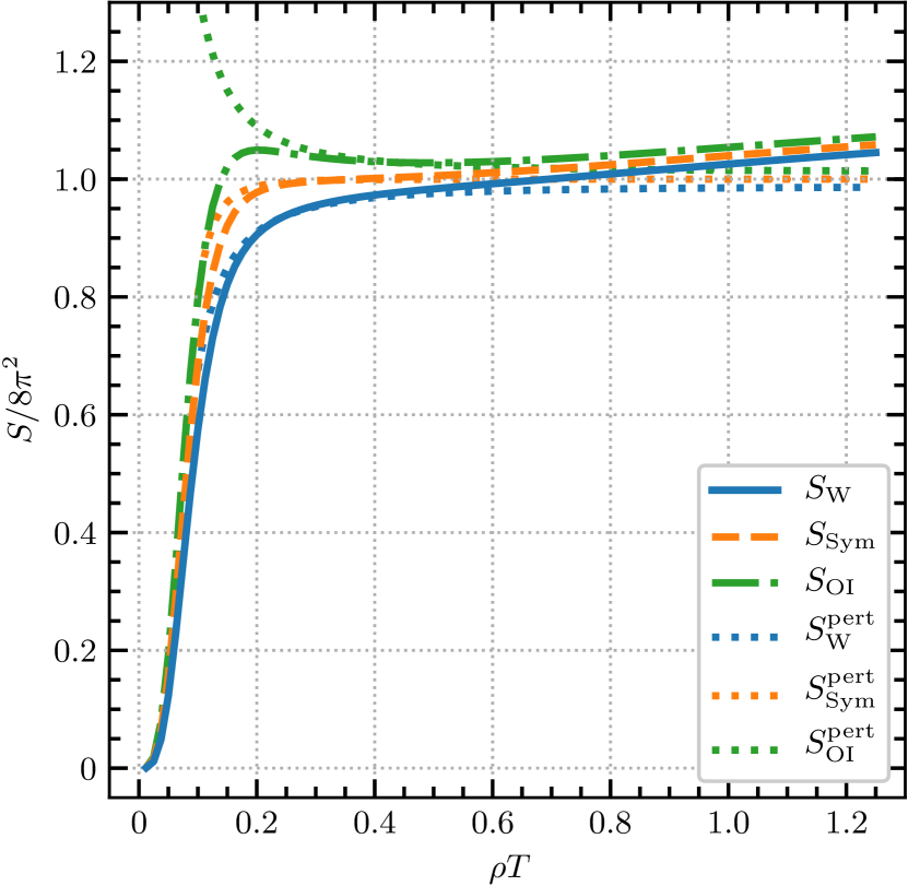
Figure 1: Different actions together with the perturbative predictions as a function of the caloron size. The caloron is placed at the center of an $8\times 48^{3}$ lattice. In this plot we used $t_{0}T^{2}=20/64$ for reducing the boundary effects (cf. App. A). Dotted lines indicate a small-$a$ expansion up to the first nontrivial correction.

The overimproved action possesses positive $a^{2}$ corrections and therefore develops a maximum. This will be of importance when flowing with this action as it will stabilize calorons larger than the size where $S$ is maximum, preventing them from shrinking, “falling through the lattice,” and being lost. As we will see, although promising, this approach does not substantially help in the calculation of the topological susceptibility.

The figure also features a rise in the action above $8\pi^{2}$ at large caloron sizes; for the lattice considered in the figure, this effect becomes larger than the $a^{2}$ effects above about $\rho T=0.7$. This is a finite-volume effect which is ameliorated by going to a larger aspect ratio. It is also partly an artifact of the way we construct the caloron solution, since we take properly into account the temporal periodicity but not the space periodicity. In order to reduce this effect as much as possible, we “flow the boundaries away.” What this means is that we perform a space-time dependent flow where the core of the configuration (where most of the topological charge is localized) is unaffected while boundary effects are smoothed out. A similar idea was used in Ref. GarciaPerez:1998ru where a discretized version of $D_{\mu}F_{\mu\nu}(x)$ was measured on every space-time point and an improved form of cooling was performed on those lattice points that satisfied the bound $D_{\mu}F_{\mu\nu}(x)>\epsilon$. In App. A we explain our own procedure for reducing boundary effects which we utilize throughout this work. From now on, when setting up a topological configuration, we always implicitly apply this procedure. Note that the gradient flow used to reduce the boundary effects should not be confused with the usual gradient flow that we apply for some calculations in the remainder of this work.

4.2 Topological Charges

The field-strength tensor $F_{\mu\nu}(x)$ is the main building block for constructing gauge operators like the topological charge. Apart from the popular geometrical clover definition (4-plaquette average), we considered an improved version thereof. To this end, we implement an improved field-strength tensor $\hat{F}^{\mathrm{imp}}_{\mu\nu}$ free of $\mathcal{O}\mathopen{}\mathclose{{}\left(a^{2}}\right)$ errors by considering weighted averages of $1\times 1$ plaquettes and $2\times 1$ rectangles Moore:1996wn ; BilsonThompson:2002jk .

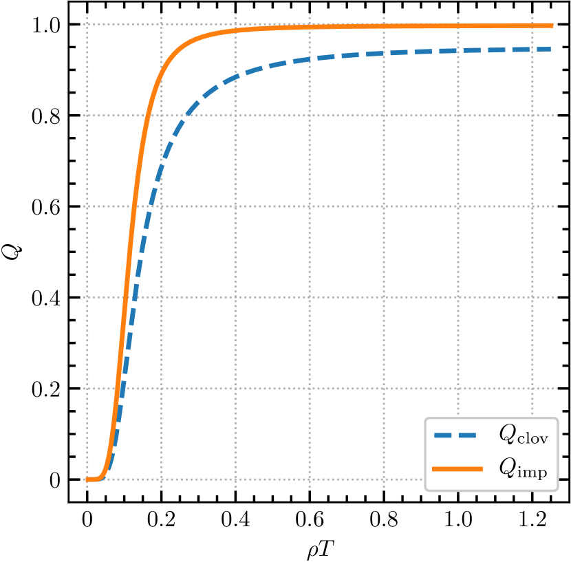
Figure 2: Two different discretizations of the topological charge operator as a function of the caloron size on an $8\times 32^{3}$ lattice.

We then study the two definitions

$$Q_{\mathrm{clov/imp}}=-\frac{1}{32\pi^{2}}\epsilon_{\mu\nu\rho\sigma}\sum_{x}\mathrm{tr}\mathopen{}\mathclose{{}\left(\hat{F}_{\mu\nu}(x)\hat{F}_{\rho\sigma}(x)}\right),$$ (17)

where in each case

$$\begin{split}\hat{F}^{\mathrm{clov}}_{\mu\nu}(x)&=F_{\mu\nu}(x)+\mathcal{O}\mathopen{}\mathclose{{}\left(a^{2}}\right),\\ \hat{F}^{\mathrm{imp}}_{\mu\nu}(x)&=F_{\mu\nu}(x)+\mathcal{O}\mathopen{}\mathclose{{}\left(a^{4}}\right).\end{split}$$ (18)

As can be seen from Fig. 2, the improved topological charge operator shows a much better behavior at all investigated values of the radius. Notice that boundary effects are milder for the topological charge than for the action. We see only advantages to using the improved definition.

4.3 Critical Radius

One of the relevant aspects we want to address in this paper is the behavior of a discretized caloron configuration under different flow equations. We see in Fig. 2 that, for $N_{\tau}=8$, a caloron with $\rho T\gtrsim 0.12$ will have a $Q$ value larger than $1/2$, if the measurement is made before any flow is applied. Of course in practice such a measurement would be impossible, since the $Q$ of the caloron would be swamped by contributions from nontopological fluctuations. These disappear after a modest amount of gadient flow. But calorons also shrink and tend to disappear as flow is applied, precisely because of the action corrections which we explored in Fig. 1. We illustrate this effect in Fig. 3, which shows how the $Q$ value changes under flow for a “large” caloron with $\rho T=0.5$ on an $N_{\tau}=8$ lattice. We see that, after some amount of time, the measured topological charge abruptly collapses. This occurs because flow causes the caloron to shrink, eventually abruptly shrinking away and disappearing between lattice sites. At least for Wilson and Zeuthen flow, any caloron will eventually disappear in this way.

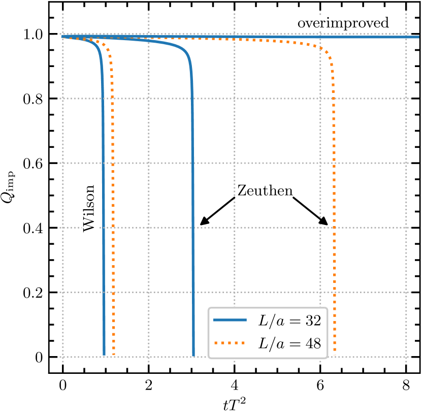
Figure 3: Topological charge $Q_{\mathrm{imp}}$ as a function of flow time for a caloron with $\rho T=0.5$, for three flow definitions and two box sizes ($N_{\tau}=8$ is fixed). Calorons live much longer under Zeuthen flow, and forever under overimproved flow.

The collapse is slower for Zeuthen flow because of the absence of $a^{2}$ lattice-spacing corrections to the action, but the $a^{4}$ and finite-volume effects nevertheless eventually lead to collapse. For the overimproved action, the action has a maximum which prevents flow from ever destroying the caloron.

It would be very useful to know more precisely, how much flow destroys what size of caloron. To investigate this, we first establish a definition of when we consider a caloron to really exist: when the topological charge $Q$ exceeds some threshold, which we choose to be $1/2$. (We see in Fig. 3 that the exact choice is almost immaterial.) This corresponds well to the typical procedure one will use in determining the topological susceptibility in a simulation: a configuration is generated, $Q$ is measured, and then its value is thresholded to an integer. The choice $1/2$ corresponds to thresholding to the nearest integer. We therefore define the critical radius of a caloron where it becomes topological as

$$Q_{\mathrm{imp}}\mathopen{}\mathclose{{}\left(\rho_{\mathrm{crit}}}\right)\equiv 0.5.$$ (19)

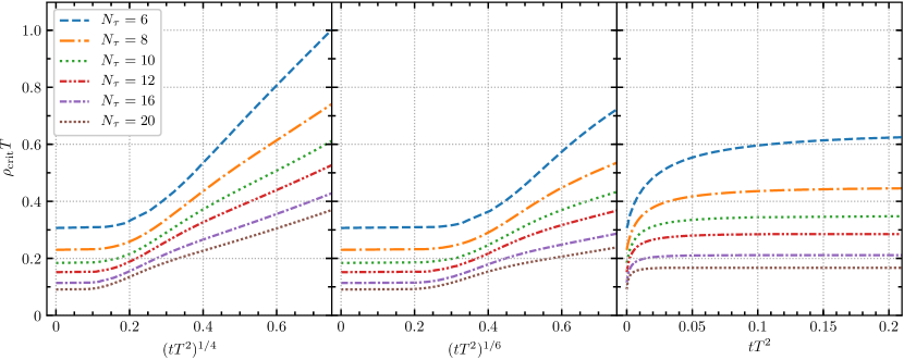
Figure 4: Critical caloron radius (separating calorons which survive from those which collapse) as a function of flow depth for three types of flow, and several different temporal lattice extents. Left: Wilson flow. Middle: Zeuthen flow. Right: Overimproved flow.

We can then study how flow causes lattice calorons to shrink and disappear by investigating $\rho_{\mathrm{crit}}$ as a function of flow time, that is, what initial caloron radii $\rho$ still have $Q_{\mathrm{imp}}>0.5$ after some flow depth $t$. This is shown in Fig. 4, which can be used to look up how much flow is needed to collapse calorons of a given size.

We see in the figure that $\rho_{\mathrm{crit}}$ grows almost linearly with $t^{1/4}$, which is easily explained analytically. An ordinary perturbative fluctuation of momentum $p$ decays as $\exp\mathopen{}\mathclose{{}\left(-p^{2}t}\right)$ (this is a leading result coming from Eq. (6)), and so doubling the size requires four times the flow time, or $t\propto\rho^{2}$. However, calorons are nearly extrema of the action, up to $a^{2}/\rho^{2}$ corrections in the Wilson action, so we expect $t\propto\rho_{\mathrm{crit}}^{4}$. Therefore Fig. 4 plots $\rho_{\mathrm{crit}}$ against $t^{1/4}$ (Wilson case), which would be a straight line for $1/N_{\tau}\ll\rho T\ll 1$. The figure shows that calorons also collapse under Zeuthen flow, though more slowly (as the energy depends on scale only at $\mathcal{O}\mathopen{}\mathclose{{}\left(a^{4}}\right)$, we therefore expect $t\propto\rho_{\mathrm{crit}}^{6}$) and, in fact, the curves show a linear trend. Under overimproved flow calorons are preserved above some critical size, which was the original motivation for considering it GarciaPerez:1993lic .

5 Estimated $a^{2}$ Errors in the Topological Susceptibility

We want to apply our results to get a semi-analytical understanding of how both flow depth and $a^{2}$ errors may influence lattice determinations of the topological susceptibility at high temperatures. Our goal is not to calculate the topological susceptibility per se, but to see how flow and lattice spacing may influence its determination at finite lattice spacing.

We will do so by approximating the distribution of topological objects using the dilute instanton gas (DIGA) approximation. We incorporate the known one-loop renormalization contributions to the caloron Gross:1980br , and estimate the topological susceptibility by integrating over all instanton sizes. In the continuum this quantity is given by

$$\chi\mathopen{}\mathclose{{}\left(T/T_{\mathrm{c}}}\right)\simeq 2\int^{1/\Lambda^{N_{\mathrm{f}}=0}_{\overline{\mathrm{MS}}}}_{0}\mathrm{d}\rho\,D(\rho)G(\pi\rho T)$$ (20)

with

$$D(\rho)=\frac{d_{\overline{\mathrm{MS}}}}{\rho^{5}}\mathopen{}\mathclose{{}\left(\frac{8\pi^{2}}{g^{2}(\mu=\rho^{-1})}}\right)^{6}\exp\mathopen{}\mathclose{{}\left(-\frac{8\pi^{2}}{g^{2}(\mu=\rho^{-1})}}\right)$$ (21)

the vacuum density of instantons with size $\rho$, and

$$G(\lambda) =\exp\mathopen{}\mathclose{{}\left(-2\lambda^{2}-18A(\lambda)}\right),$$ (22)

$$A(\lambda) =-\frac{1}{12}\ln\mathopen{}\mathclose{{}\left(1+\frac{\lambda^{2}}{3}}\right)+\alpha\mathopen{}\mathclose{{}\left(1+\gamma\lambda^{-\frac{3}{2}}}\right)^{-8}$$ (23)

the thermal corrections, first computed by Gross, Pisarski, and Yaffe Gross:1980br . The parameter values in these expressions are $\alpha=0.0128974$, $\gamma=0.15858$, and $d_{\overline{\mathrm{MS}}}=\frac{\mathrm{e}^{5/6}}{\pi^{2}}\mathrm{e}^{-4.534122}$. The running of the coupling $g^{2}(\mu)$ can be found in Ref. Chetyrkin:1997un and $T_{\mathrm{c}}/\Lambda^{N_{\mathrm{f}}=0}_{\overline{\mathrm{MS}}}=1.26$ is taken from Ref. Borsanyi:2012ve . The product of $D(\rho)$ and of $G(\pi\rho T)$ in Eq. (20) leads to an integrand with a broad peak near $\rho T\simeq 0.4$ (solid black curve in Fig. 5), which is then the typical size for the calorons which dominate the topological susceptibility.

In performing a lattice Monte-Carlo study, the practitioner chooses an action for sampling configurations. The choice is logically independent from the choice of action used in gradient flow, but it can be equally impactful. In particular, if the lattice study is based on sampling with the Wilson action, something we assume throughout this section, then the continuum action $8\pi^{2}$ in Eq. (21) should be replaced by the lattice Wilson action of a caloron from Eq. (15), leading to an $a^{2}$ correction to $D(\rho)$:

$$D_{\mathrm{lat}}(\rho,T/T_{\mathrm{c}},N_{\tau})=$$

$$D(\rho)\exp\mathopen{}\mathclose{{}\left[-\frac{8\pi^{2}}{g^{2}(\mu=\rho^{-1})}\mathopen{}\mathclose{{}\left(\frac{1}{\rho TN_{\tau}}}\right)^{2}\mathcal{F}\mathopen{}\mathclose{{}\left(\rho T}\right)}\right].$$ (24)

This rests on an assumption that the coefficient in front of the dimension-6 $a^{2}$-suppressed operator ($DFDF$) takes its tree level value. Realistically we expect corrections from, e.g., the renormalization of the $a^{2}$ action correction and from higher-order effects in $G(\pi\rho T)$, so our results here should be viewed only as estimates, based on the best tools we have available, for how $a^{2}$ effects will affect the caloron density on the lattice.

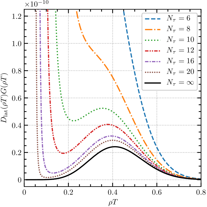
Figure 5: Integrand of Eq. (25) at $T/T_{\mathrm{c}}=4$ for $N_{\tau}=6,8,10,12,16,20$. The black solid curve represents the continuum case and corresponds to the intregrand of Eq. (20).

To estimate the topological susceptibility as measured on the lattice, we integrate this modified caloron density over those caloron sizes which are not destroyed by gradient flow – which is precisely all $\rho>\rho_{\mathrm{crit}}$ as determined in Fig. 4. We therefore write

$$\chi_{\mathrm{lat}}(T/T_{\mathrm{c}},N_{\tau},tT^{2})=$$

$$2\int^{1/\Lambda^{N_{\mathrm{f}}=0}_{\overline{\mathrm{MS}}}}_{\rho_{\mathrm{crit}}(tT^{2},N_{\tau})}\mathrm{d}\rho\,D_{\mathrm{lat}}\mathopen{}\mathclose{{}\left(\mu=\rho^{-1},T/T_{\mathrm{c}}}\right)G(\pi\rho T).$$ (25)

We illustrate the integrand for several $N_{\tau}$ values in Fig. 5.

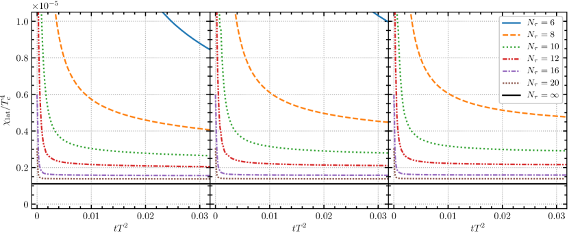
Figure 6: Estimated effect of lattice artifacts on the topological susceptibility, at $T/T_{\mathrm{c}}=4$ and for $N_{\tau}=6,8,10,12,16,20$, as a function of the flow depth $tT^{2}$. Left: Wilson flow. Middle: Zeuthen flow. Right: Overimproved flow. The solid line denotes the continuum limit.

Fig. 6 shows the resulting estimate of the topological susceptibility which we would obtain by working at a given $N_{\tau}$ and applying a given amount of gradient flow. The lattice corrections to the action raise the contributions in the peak of Eq. (20) near $\rho T\simeq 0.4$. But lattice artifacts also dramatically increase the number of dislocations with $\rho\sim a$, as we see from the integrand in Fig. 5. If these two scales, $a$ and $0.4/T$, are well separated, then gradient flow can erase the dislocations with little impact on the typical calorons. That is, there will be a minimum in the integrand of Fig. 5, and we can use Fig. 4 to choose a flow depth which will erase calorons below this minimum. This leads to a plateau in the susceptibility over a range of flow depths, as seen in Fig. 6. For coarser lattices such as $N_{\tau}=6,8$, examining Fig. 5, it is not clear where to cut to separate calorons from dislocations, and there is no associated plateau in Fig. 6. Therefore $N_{\tau}=6,8$ will likely not be sufficient to give results which are stable against the amount of flow, but larger $N_{\tau}$ will, especially if we use Zeuthen flow. Overimproved flow is good for completely “cleaning” a configuration of perturbative fluctuations, but in terms of eliminating small instantons, it is effectively equivalent to using a specific fixed depth of Wilson flow. Therefore it is not preferred if we want flexibility in choosing the size of caloron/dislocation which we eliminate.

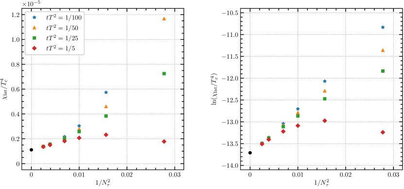
Figure 7: Left: Continuum extrapolation Eq. (25) at $T/T_{\mathrm{c}}=4$ at fixed (Wilson) flow time. Right: Logarithm of left plot. The black point represents the continuum value.

Finally, we consider the extrapolation to zero lattice spacing in Fig. 7. The lattice spacing corrections are very large even for $N_{\tau}=10$, and a simple extrapolation in $\chi$ can easily lead to a negative result. But that is because the $a^{2}$ errors are best viewed as a correction to the logarithm of $\chi$, as we see in Eq. (5). If we extrapolate in terms of $\ln(\chi)$, the procedure works much better.

6 Conclusions

We have constructed calorons on the lattice. We find that they possess most of the action and topological charge if $\rho T\gtrsim 1/N_{\tau}$, and nearly all of the charge and action if $\rho T\gtrsim 2/N_{\tau}$. Wilson flow destroys small calorons, with progressively more flow destroying larger calorons, as expected. Our work expresses this in a quantitative fashion, in Fig. 4.

Also, if a lattice study were to flow each topologically nontrivial configuration until it loses topological character ($Q_{\mathrm{imp}}<0.5$), and keep track of the distribution of flow depths needed, then a plot as the one in Fig. 3 could be used to turn this result into a size distribution of the topological objects observed on the lattice.

Using our results to estimate the $a^{2}$ errors which arise when computing the topological susceptibility $\chi(T)$ on the lattice, we find that $N_{\tau}=6$ is insufficient to be in the scaling regime (probably $N_{\tau}=8$ as well), and lattice spacing errors are expected to lead to a severe overestimate of $\chi(T)$ at finite $a$, which may lead to negative values if we extrapolate $\chi(T)$ against $a^{2}$. It is more natural to extrapolate $\ln\mathopen{}\mathclose{{}\left(\chi(T)}\right)$ against $a^{2}$, because this corresponds better to the way in which $a^{2}$ errors enter in the susceptibility.

Note that the inclusion of light quarks in Eq. (22) would change the factor $-2\lambda^{2}$ to $-(2+N_{\mathrm{f}}/3)\lambda^{2}$, which makes the dominant size of calorons smaller. Therefore, since $\rho TN_{\tau}$ becomes smaller, the corrections in Eq. (5) become larger (since $\mathcal{F}$ is negative), and the value of $N_{\tau}$ needed to reach scaling will be still larger.

Appendix A Reducing Boundary Effects

In writing down caloron field configurations, we cannot avoid the discontinuity at the spatial boundaries of our box. We will try to minimize the damage by smearing out the boundary discontinuities with gradient flow. Consider the caloron placed at the center of the lattice and denote the lattice spatial extent as $L$. We then flow the links using a flow time that depends on the relative distance

$$d=\sqrt{\mathopen{}\mathclose{{}\left(x-z}\right)^{2}}$$ (26)

of the base point of the link $U_{\mu}(x)$ and the center of the instanton. The flow time depth gets modified as

$$t(d)=\begin{cases}0,\hfill d<\frac{L}{4}\\ \frac{t_{0}}{2}\mathopen{}\mathclose{{}\left(1+\sin\mathopen{}\mathclose{{}\left[\frac{4\pi}{L}\mathopen{}\mathclose{{}\left(d-\frac{3}{8}L}\right)}\right]}\right),\hfill\frac{L}{4}\leq d\leq\frac{L}{2}\\ t_{0},\hfill d>\frac{L}{2}\end{cases}$$ (27)

where $t_{0}$ is the “normal” flow time. This is nothing but a smooth interpolation between zero flow (close to the center of the caloron) and full flow (close to the boundary). With this procedure we reduce boundary effects while the core of the caloron remains unaffected. In Fig. 8 we show both the topological charge and the Wilson action of the caloron for different values of $t_{0}$. We observe that the Wilson action suffers significantly more from boundary effects than the topological charge. Applying this modified version of Wilson flow indeed reduces boundary effects. We find that a flow time of $t_{0}T^{2}=5/N^{2}_{\tau}$ is sufficient to satisfactorily reduce most of the boundary effects.

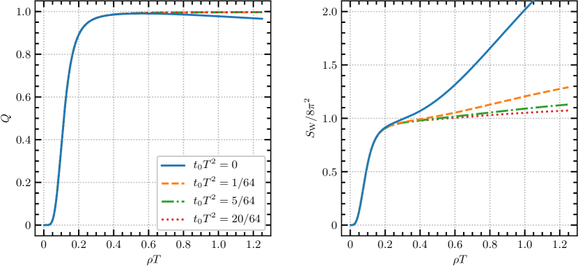
Figure 8: Caloron topological charge (left) and Wilson action (right) for different values of $t_{0}T^{2}$ as defined in Eq. (27) on an $8\times 48^{3}$ lattice.

References

- (1) T. Schäfer and E. V. Shuryak, Instantons in QCD, Rev. Mod. Phys. 70 (1998) 323–426, [hep-ph/9610451].
- (2) R. Peccei and H. R. Quinn, Constraints Imposed by CP Conservation in the Presence of Instantons, Phys.Rev. D16 (1977) 1791–1797.
- (3) S. Weinberg, A New Light Boson?, Phys.Rev.Lett. 40 (1978) 223–226.
- (4) F. Wilczek, Problem of Strong p and t Invariance in the Presence of Instantons, Phys.Rev.Lett. 40 (1978) 279–282.
- (5) J. Preskill, M. B. Wise and F. Wilczek, Cosmology of the Invisible Axion, Phys. Lett. B120 (1983) 127–132.
- (6) L. F. Abbott and P. Sikivie, A Cosmological Bound on the Invisible Axion, Phys. Lett. B120 (1983) 133–136.
- (7) M. Dine and W. Fischler, The Not So Harmless Axion, Phys. Lett. B120 (1983) 137–141.
- (8) G. Grilli di Cortona, E. Hardy, J. P. Vega and G. Villadoro, The QCD axion, precisely, JHEP 01 (2016) 034, [1511.02867].
- (9) V. B. Klaer and G. D. Moore, The dark-matter axion mass, JCAP 1711 (2017) 049, [1708.07521].
- (10) G. D. Moore, Axion dark matter and the Lattice, EPJ Web Conf. 175 (2018) 01009, [1709.09466].
- (11) E. Berkowitz, M. I. Buchoff and E. Rinaldi, Lattice QCD input for axion cosmology, Phys. Rev. D92 (2015) 034507, [1505.07455].
- (12) S. Borsanyi, M. Dierigl, Z. Fodor, S. D. Katz, S. W. Mages, D. Nogradi et al., Axion cosmology, lattice QCD and the dilute instanton gas, Phys. Lett. B752 (2016) 175–181, [1508.06917].
- (13) P. Petreczky, H.-P. Schadler and S. Sharma, The topological susceptibility in finite temperature QCD and axion cosmology, Phys. Lett. B762 (2016) 498–505, [1606.03145].
- (14) Y. Taniguchi, K. Kanaya, H. Suzuki and T. Umeda, Topological susceptibility in finite temperature ( 2+1 )-flavor QCD using gradient flow, Phys. Rev. D95 (2017) 054502, [1611.02411].
- (15) F. Burger, E.-M. Ilgenfritz, M. P. Lombardo, M. Müller-Preussker and A. Trunin, Topology (and axion’s properties) from lattice QCD with a dynamical charm, Nucl. Phys. A967 (2017) 880–883, [1705.01847].
- (16) J. Frison, R. Kitano, H. Matsufuru, S. Mori and N. Yamada, Topological susceptibility at high temperature on the lattice, JHEP 09 (2016) 021, [1606.07175].
- (17) S. Borsanyi et al., Calculation of the axion mass based on high-temperature lattice quantum chromodynamics, Nature 539 (2016) 69–71, [1606.07494].
- (18) P. T. Jahn, G. D. Moore and D. Robaina, in pure-glue QCD through reweighting, Phys. Rev. D98 (2018) 054512, [1806.01162].
- (19) I. G. Irastorza and J. Redondo, New experimental approaches in the search for axion-like particles, 1801.08127.
- (20) D. J. Gross, R. D. Pisarski and L. G. Yaffe, QCD and Instantons at Finite Temperature, Rev. Mod. Phys. 53 (1981) 43.
- (21) A. D. Linde, Infrared Problem in Thermodynamics of the Yang-Mills Gas, Phys. Lett. 96B (1980) 289–292.
- (22) M. Lüscher, Topology of Lattice Gauge Fields, Commun. Math. Phys. 85 (1982) 39.
- (23) P. H. Ginsparg and K. G. Wilson, A Remnant of Chiral Symmetry on the Lattice, Phys. Rev. D25 (1982) 2649.
- (24) H. Neuberger, Exactly massless quarks on the lattice, Phys. Lett. B417 (1998) 141–144, [hep-lat/9707022].
- (25) M. Luscher, Exact chiral symmetry on the lattice and the Ginsparg-Wilson relation, Phys. Lett. B428 (1998) 342–345, [hep-lat/9802011].
- (26) R. Narayanan and H. Neuberger, Infinite N phase transitions in continuum Wilson loop operators, JHEP 03 (2006) 064, [hep-th/0601210].
- (27) M. Lüscher, Trivializing maps, the Wilson flow and the HMC algorithm, Commun. Math. Phys. 293 (2010) 899–919, [0907.5491].
- (28) B. Berg, Dislocations and Topological Background in the Lattice O(3) Model, Phys. Lett. B104 (1981) 475–480.
- (29) P. de Forcrand, M. Garcia Perez and I.-O. Stamatescu, Topology of the SU(2) vacuum: A Lattice study using improved cooling, Nucl. Phys. B499 (1997) 409–449, [hep-lat/9701012].
- (30) M. Garcia Perez, O. Philipsen and I.-O. Stamatescu, Cooling, physical scales and topology, Nucl. Phys. B551 (1999) 293–313, [hep-lat/9812006].
- (31) M. Garcia Perez, A. Gonzalez-Arroyo, A. Montero and P. van Baal, Calorons on the lattice: A New perspective, JHEP 06 (1999) 001, [hep-lat/9903022].
- (32) M. Teper, Instantons in the Quantized SU(2) Vacuum: A Lattice Monte Carlo Investigation, Phys. Lett. B162 (1985) 357–362.
- (33) B. J. Harrington and H. K. Shepard, Periodic Euclidean Solutions and the Finite Temperature Yang-Mills Gas, Phys. Rev. D17 (1978) 2122.
- (34) A. Ramos and S. Sint, Symanzik improvement of the gradient flow in lattice gauge theories, Eur. Phys. J. C76 (2016) 15, [1508.05552].
- (35) D. J. R. Pugh and M. Teper, Topological Dislocations in the Continuum Limit of SU(2) Lattice Gauge Theory, Phys. Lett. B224 (1989) 159–165.
- (36) F. Bruckmann, D. Nogradi and P. van Baal, Higher charge calorons with non-trivial holonomy, Nucl. Phys. B698 (2004) 233–254, [hep-th/0404210].
- (37) F. Bruckmann, E. M. Ilgenfritz, B. V. Martemyanov, M. Muller-Preussker, D. Nogradi, D. Peschka et al., Calorons with non-trivial holonomy on and off the lattice, Nucl. Phys. Proc. Suppl. 140 (2005) 635–646, [hep-lat/0408036].
- (38) P. de Forcrand, M. Garcia Perez and I.-O. Stamatescu, Improved cooling algorithm for gauge theories, Nucl. Phys. Proc. Suppl. 47 (1996) 777–780, [hep-lat/9509064].
- (39) P. de Forcrand and S. Kim, Topological susceptibility and instanton size distribution from over improved cooling, Nucl. Phys. Proc. Suppl. 47 (1996) 278–281, [hep-lat/9509081].
- (40) G. ’t Hooft, Symmetry Breaking Through Bell-Jackiw Anomalies, Phys. Rev. Lett. 37 (1976) 8–11.
- (41) R. Jackiw, C. Nohl and C. Rebbi, Conformal Properties of Pseudoparticle Configurations, Phys. Rev. D15 (1977) 1642.
- (42) M. Lüscher, Properties and uses of the Wilson flow in lattice QCD, JHEP 08 (2010) 071, [1006.4518].
- (43) M. Lüscher, Topology, the Wilson flow and the HMC algorithm, PoS LATTICE2010 (2010) 015, [1009.5877].
- (44) M. Lüscher and P. Weisz, Perturbative analysis of the gradient flow in non-abelian gauge theories, JHEP 02 (2011) 051, [1101.0963].
- (45) M. Lüscher, Chiral symmetry and the Yang–Mills gradient flow, JHEP 04 (2013) 123, [1302.5246].
- (46) M. Lüscher and P. Weisz, On-Shell Improved Lattice Gauge Theories, Commun. Math. Phys. 97 (1985) 59.
- (47) http://luscher.web.cern.ch/luscher/openQCD/index.html.
- (48) M. Garcia Perez, A. Gonzalez-Arroyo, J. R. Snippe and P. van Baal, Instantons from over - improved cooling, Nucl. Phys. B413 (1994) 535–552, [hep-lat/9309009].
- (49) G. D. Moore, Improved Hamiltonian for Minkowski Yang-Mills Theory, Nucl. Phys. B480 (1996) 689–728, [hep-lat/9605001].
- (50) S. O. Bilson-Thompson, D. B. Leinweber and A. G. Williams, Highly improved lattice field strength tensor, Annals Phys. 304 (2003) 1–21, [hep-lat/0203008].
- (51) K. G. Chetyrkin, B. A. Kniehl and M. Steinhauser, Decoupling relations to O (alpha-s**3) and their connection to low-energy theorems, Nucl. Phys. B510 (1998) 61–87, [hep-ph/9708255].
- (52) S. Borsanyi, G. Endrodi, Z. Fodor, S. D. Katz and K. K. Szabo, Precision SU(3) lattice thermodynamics for a large temperature range, JHEP 07 (2012) 056, [1204.6184].