Efficient Bayesian Inference for a Gaussian Process Density Model

Abstract

We reconsider a nonparametric density model based on Gaussian processes. By augmenting the model with latent Pólya–Gamma random variables and a latent marked Poisson process we obtain a new likelihood which is conjugate to the model’s Gaussian process prior. The augmented posterior allows for efficient inference by Gibbs sampling and an approximate variational mean field approach. For the latter we utilise sparse GP approximations to tackle the infinite dimensionality of the problem. The performance of both algorithms and comparisons with other density estimators are demonstrated on artificial and real datasets with up to several thousand data points.

1 INTRODUCTION

Gaussian processes (GP) provide highly flexible nonparametric prior distributions over functions [1]. They have been successfully applied to various statistical problems such as e.g. regression [2], classification [3], point processes [4] or the modelling of dynamical systems [5, 6]. Hence, it would seem natural to apply Gaussian processes also to density estimation which is one of the most basic statistical problems. GP density estimation, however, is a nontrivial task: Typical realisations of a GP do not respect non–negativity and normalisation of a probability density. Hence, functions drawn from a GP prior have to be passed through a nonlinear squashing function and the results have to be normalised subsequently to model a density. These operations make the corresponding posterior distributions non–Gaussian. Moreover, likelihoods depend on all the infinitely many GP function values in the domain rather than on the finite number of function values at observed data points. Since analytical inference is impossible, [7] introduced an interesting Markov chain Monte–Carlo sampler which allows for (asymptotically) exact inference for a Gaussian process density model, where the GP is passed through a sigmoid link function. The approach is able to deal with the infinite dimensionality of the model, because the sampling of the GP variables is reduced to a finite dimensional problem by a point process representation. However, since the likelihood of the GP variables is not conjugate to the prior, the method has to resort to a time–consuming Metropolis–Hastings approach. In this paper we will use recent results on representing the sigmoidal squashing function as an infinite mixture of Gaussians involving Pólya–Gamma random variables [9] to augment the model in such a way that the model becomes tractable by a simpler Gibbs sampler. The new model structure allows also for a much faster variational Bayesian approximation.

The paper is organised as follows: Sec. 2 introduces the GP density model, followed by an augmentation scheme that makes its likelihood conjugate to the GP prior. With this model representation we derive two efficient Bayesian inference algorithms in Sec. 3, namely an exact Gibbs sampler and an approximate, fast variational Bayes algorithm. The performance of both algorithms is demonstrated in Sec. 4 on artificial and real data. Finally, Sec. 5 discusses potential extensions of the model.

2 GAUSSIAN PROCESS DENSITY MODEL

The generative model proposed by [7] constructs densities over some $d$-dimensional data space $\mathcal{X}$ to be of the form

$$\rho(\boldsymbol{x}|g)=\frac{\sigma(g(\boldsymbol{x}))\pi(\boldsymbol{x})}{\int_{\mathcal{X}}\sigma(g(\boldsymbol{x}))\pi(\boldsymbol{x})d\boldsymbol{x}}.$$ (1)

$\pi(\boldsymbol{x})$ defines a (bounded) base probability measure over $\mathcal{X}$, which is usually taken from a fixed parametric family. The denominator ensures normalisation $\int_{\mathcal{X}}\rho(\boldsymbol{x}|g)d\boldsymbol{x}=1$. The choice of $\pi(\boldsymbol{x})$ is important as will be discussed Sec. 5. A prior distribution over densities is introduced by assuming a Gaussian process prior [1] over the function $g(\boldsymbol{x}):\mathcal{X}\rightarrow\mathbb{R}$. The GP is defined by a mean function $\mu(\boldsymbol{x})$ (in this paper, we consider only constant mean functions $\mu(\boldsymbol{x})=\mu_{0}$) and covariance kernel $k(\boldsymbol{x},\boldsymbol{x}^{\prime})$. Finally, $\sigma(z)=\frac{1}{1+e^{-z}}$ is the sigmoid function, which guarantees that the density is non–negative and bounded.

In Bayesian inference, the posterior distribution of $g$ given observed data ${\cal D}=\left\{\boldsymbol{x}_{n}\right\}_{n=1}^{N}$ with $\boldsymbol{x}\in\mathcal{X}$ is computed from the GP prior $p(g)$ and the likelihood as

$$p(g|{\cal D})\propto p({\cal D}|g)p(g).$$ (2)

The likelihood is given by

$$p({\cal D}|g)=\frac{\prod_{n=1}^{N}\sigma(g(\boldsymbol{x}_{n}))\pi(\boldsymbol{x}_{n})}{\left(\int_{\mathcal{\mathcal{X}}}\sigma(g(\boldsymbol{x}))\pi(\boldsymbol{x})d\boldsymbol{x}\right)^{N}}.$$ (3)

Practical inference for this problem, however, is non-trivial, because (i) the posterior is non–Gaussian and (ii) the likelihood involves an integral of $g$ over the whole space. Thus, in contrast to simpler problems such as GP regression or classification, it is impossible to reduce inference to finite dimensional integrals. To circumvent the problem that the likelihood is not conjugate to the GP prior, [7] proposed a Metropolis-Hastings MCMC algorithm for this model. We will show in the next sections that one can augment the model with auxiliary latent random variables in such a way that the resulting likelihood is of a conjugate form allowing for a more efficient Gibbs sampler with explicit conditional probabilities.

2.1 LIKELIHOOD AUGMENTATION

To obtain a likelihood which is conjugate to the GP $p(g)$ we require that it assumes a Gaussian form in $g$.

Representing the denominator

As a starting point, we follow [10] and use the representation

$$\frac{1}{z^{N}}=\frac{\int_{0}^{\infty}\lambda^{N-1}e^{-\lambda z}d\lambda}{\Gamma(N)},$$ (4)

where $\Gamma(\cdot)$ is the gamma function. Identifying $z=\int_{\mathcal{\mathcal{X}}}\sigma(g(\boldsymbol{x}))\pi(\boldsymbol{x})d\boldsymbol{x}$ in Eq. (3) we can rewrite the likelihood as $p({\cal D}|g)=\int_{0}^{\infty}p({\cal D},\lambda|g)d\lambda$ where

$$\begin{split}p({\cal D},\lambda|g)\propto&\exp\left(-\int_{\mathcal{X}}\lambda\sigma(g(\boldsymbol{x}))\pi(\boldsymbol{x})d\boldsymbol{x}\right)\\ &\times p(\lambda)\;\prod_{n=1}^{N}\lambda\sigma(g(\boldsymbol{x}_{n}))\pi(\boldsymbol{x}_{n}),\end{split}$$ (5)

with the improper prior $p(\lambda)=\lambda^{-1}$ over the auxiliary latent variable $\lambda$. To transform the likelihood further into a form which is Gaussian in $g$, we utilise a representation of the sigmoid function as a scale mixture of Gaussians.

Pólya–Gamma representation of sigmoid function

As discovered by [9], the inverse hyperbolic cosine can be represented as an infinite mixture of scaled Gaussians

$$\cosh^{-b}(z/2)=\int_{0}^{\infty}e^{-\frac{z^{2}}{2}\omega}p_{\scriptscriptstyle\mathrm{PG}}(\omega|b,0)d\omega,$$ (6)

where $p_{\scriptscriptstyle\mathrm{PG}}(\omega|b,0)$ is the Pólya–Gamma density of random variable $\omega\in\mathbb{R}^{+}$. Moments of those densities can be easily computed [9]. Later, we will also use the tilted Pólya-Gamma densities defined as

$$p_{\scriptscriptstyle\mathrm{PG}}(\omega|b,c)\propto\exp\left(-\frac{c^{2}}{2}\omega\right)p_{\scriptscriptstyle\mathrm{PG}}(\omega|b,0).$$ (7)

These definitions allows for a Gaussian representation of the sigmoid function as

$$\sigma(z)=\frac{e^{z/2}}{2\cosh(z/2)}=\int_{0}^{\infty}e^{f(\omega,z)}p_{\scriptscriptstyle\mathrm{PG}}(\omega|1,0)d\omega$$ (8)

with $f(\omega,z)=\frac{z}{2}-\frac{z^{2}}{2}\omega-\ln 2$. This result will be used to transform the products over observations $\sigma(g(\boldsymbol{x}_{n}))$ in the likelihood (5) into a Gaussian form.

We will next deal with the first term in the likelihood (5) which contains the integral over $\boldsymbol{x}$. For this part of the model we will derive a point process representation which can be understood as a generalisation of the approach of [7].

Marked–Poisson representation

Utilising the sigmoid property $\sigma(z)=1-\sigma(-z)$ and the Pólya-Gamma representation (8) the integral in the exponent of Eq. (5) can be written as a double integral

$$\begin{split}&-\int_{\mathcal{X}}\lambda\sigma(g(\boldsymbol{x}))\pi(\boldsymbol{x})d\boldsymbol{x}=\\ &\int_{\mathcal{X}}(\sigma(-g(\boldsymbol{x}))-1)\lambda\pi(\boldsymbol{x})d\boldsymbol{x}=\\ &\int_{\mathcal{X}}\int_{\mathbb{R}^{+}}\left(e^{f(\omega,-g(\boldsymbol{x}))}-1\right)\lambda\pi(\boldsymbol{x})p_{\scriptscriptstyle\mathrm{PG}}(\omega|1,0)d\omega d\boldsymbol{x}\end{split}$$ (9)

Next we will use a result for the characteristic function of a Poisson process. Following [11, chap. 3] one has

$$\mathbb{E}_{\phi}\left[\prod_{\boldsymbol{z}\in\Pi}h(\boldsymbol{z})\right]=\exp\left(\int_{\mathcal{Z}}(h(\boldsymbol{z})-1)\phi(\boldsymbol{z})d\boldsymbol{z}\right).$$ (10)

$h(\cdot)$ is a function on a space $\mathcal{Z}$ and the expectation is over a Poisson process $\Pi$ with rate function $\phi(\boldsymbol{z})$. $\Pi=\left\{\boldsymbol{z}_{m}\right\}_{m=1}^{M}$ denotes a random set of points on the space $\mathcal{Z}$. To apply this result to our problem, we identify $\mathcal{Z}=\mathcal{X}\times R^{+}$, $\boldsymbol{z}=(\boldsymbol{x},\omega)$ and $\phi_{\lambda}(\boldsymbol{x},\omega)=\lambda\pi(\boldsymbol{x})p_{\scriptscriptstyle\mathrm{PG}}(\omega|1,0)$ and finally $h(\boldsymbol{z})=e^{f(\omega,-g(\boldsymbol{x}))}$ to rewrite the exponential in Eq. (5) as

$$\begin{split}e^{-\int_{\mathcal{X}}\lambda\sigma(g(\boldsymbol{x}))\pi(\boldsymbol{x})d\boldsymbol{x}}=\mathbb{E}_{{\phi}_{\lambda}}\left[\prod_{(\omega,\boldsymbol{x})\in\Pi}e^{f(\omega,-g(\boldsymbol{x}))}\right].\end{split}$$ (11)

By substituting Eq. (8) and (11) into Eq.(5) we obtain the final augmented form of the likelihood of Eq. (3) which is one of the main results of our paper.

$$\begin{split}p({\cal D},\lambda,\Pi,&\boldsymbol{\omega}_{N}|g)\propto\prod_{n=1}^{N}\phi_{\lambda}(\boldsymbol{x}_{n},\omega_{n})e^{f(\omega_{n},g(\boldsymbol{x}_{n}))}\\ &\times p_{\phi_{\lambda}}(\Pi|\lambda)p(\lambda)\;\prod_{(\omega,\boldsymbol{x})\in\Pi}e^{f(\omega,-g(\boldsymbol{x}))},\end{split}$$ (12)

with $p_{\phi}(\Pi|\lambda)$ being the density over a Poisson process $\Pi=\left\{(\boldsymbol{x}_{m},\omega_{m})\right\}_{m=1}^{M}$ in the augmented space $\mathcal{X}\times\mathbb{R}^{+}$ with intensity $\phi_{\lambda}(\boldsymbol{x},\omega)$. This new process can be identified as a marked Poisson process [11, chap. 5], where the events $\left\{\boldsymbol{x}_{m}\right\}_{m=1}^{M}$ in the original data space $\mathcal{X}$ follow a Poisson process with rate $\lambda\pi(\boldsymbol{x})$. Then, on each event $\boldsymbol{x}_{m}$ an independent mark $\omega_{m}\sim p_{\scriptscriptstyle\mathrm{PG}}(\omega_{m}|b,0)$ is drawn at random from the Pólya–Gamma density. Finally, $\boldsymbol{\omega}_{N}=\left\{\omega_{n}\right\}_{n=1}^{N}$ is the set of latent Pólya–Gamma variables which result from the sigmoid augmentation at the observations $\boldsymbol{x}_{n}$.

Augmented posterior over GP density

With Eq. (12) we obtain the joint posterior over the GP $g$, the rate scaling $\lambda$, the marked Poisson process $\Pi$, and the Pólya–Gamma variables at the observations $\boldsymbol{\omega}_{N}$ as

$$p(\boldsymbol{\omega}_{N},\Pi,\lambda,g|{\cal D})\propto p({\cal D},\boldsymbol{\omega}_{N},\Pi,\lambda|g)p(g).$$ (13)

In the following, this new representation will be used to derive two inference algorithms.

3 INFERENCE

We will first derive an efficient Gibbs sampler which (asymptotically) solves the inference problem exactly, and then a variational mean-field algorithm, which only finds an approximate solution, but in a much faster time.

3.1 GIBBS SAMPLER

Gibbs sampling [13] generates samples from the posterior by creating a Markov chain, where at each time, a block of variables is drawn from the conditional posterior given all the other variables. Hence, to perform Gibbs sampling, we have to derive these conditional distributions for each set of variables from Eq. (13). Most of the following results are easily obtained by direct inspection. The only non–trivial case is the conditional distribution over the latent point process $\Pi$.

Pólya-Gamma variables at observations

The conditional posterior over the set of Pólya–Gamma variables $\boldsymbol{\omega}_{N}$ depends only on the function $g$ at the observations $\left\{g(\boldsymbol{x}_{n})\right\}_{n=1}^{N}$ and turns out to be

$$p(\boldsymbol{\omega}_{N}|\boldsymbol{g})=\prod_{n=1}^{N}p_{\scriptscriptstyle\mathrm{PG}}(\omega_{n}|1,g(\boldsymbol{x}_{n})),$$ (14)

where we have used the definition of a tilted Pólya-Gamma density in Eq. (7). This density can be efficiently sampled by methods developed by [9].

Rate scaling

The rate scaling $\lambda$ has a conditional Gamma density given by

$$\rm{Gamma}(\lambda|\alpha,1)=\frac{(\lambda)^{\alpha-1}e^{-\lambda}}{\Gamma(\alpha)}.$$ (15)

with $\alpha=|\Pi|+N=M+N$. Hence, the posterior is dependent on the number of observations and the number on events of the marked Poisson process $\Pi$.

Posterior Gaussian process

Due to the form of the augmented likelihood the conditional posterior for the GP $\boldsymbol{g}_{N+M}$ at the observations $\left\{\boldsymbol{x}_{n}\right\}_{n=1}^{N}$ and the latent events $\left\{\boldsymbol{x}_{m}\right\}_{m=1}^{M}$ is a multivariate Gaussian density

$$p(\boldsymbol{g}_{N+M}|\Pi,\boldsymbol{\omega}_{N})=\mathcal{N}(\boldsymbol{\mu}_{N+M},\Sigma_{N+M}),$$ (16)

with covariance matrix $\Sigma_{N+M}=[D+K_{N+M}^{-1}]^{-1}$. The diagonal matrix $D$ has its first $N$ entries given by $\boldsymbol{\omega}_{N}$ followed by $M$ entries being $\left\{\omega_{m}\right\}_{m=1}^{M}$. The mean is $\boldsymbol{\mu}_{N+M}=\Sigma_{N+M}\left[\boldsymbol{u}+K_{N+M}^{-1}\boldsymbol{\mu}_{0}^{(N+M)}\right]$, where the first $N$ entries of $N+M$ dimensional vector $\boldsymbol{u}$ are $1/2$ and the rest are $-1/2$. $K_{N+M}$ is the prior covariance kernel matrix of the GP evaluated at the observed points $\boldsymbol{x}_{n}$ and the latent events $\boldsymbol{x}_{m}$, and $\boldsymbol{\mu}_{0}^{(N+M)}$ is an $N+M$ dimensional vector with all entries being $\mu_{0}$.

The predictive conditional posterior for the GP for any set of points in $\mathcal{X}$ is simply given via the conditional prior $p(g|\boldsymbol{g}_{N+M})$, which has a well known form and can be found in [1].

Sampling the latent marked point process

We easily find that the conditional posterior of the marked point process is given by

$$\scriptstyle p(\Pi|g,\lambda)= \scriptstyle\frac{\prod_{\omega,\boldsymbol{x}\in\Pi}e^{f(\omega,-g(\boldsymbol{x}))}p_{\phi_{\lambda}}(\Pi|\lambda)}{\exp\left(\int_{\mathcal{X}\times\mathbb{R}^{+}}\left(e^{f(\omega,-g(\boldsymbol{x}))}-1\right)\phi_{\lambda}(\boldsymbol{x},\omega)d\omega d\boldsymbol{x}\right)},$$ (17)

where the form of the normalising denominator is obtained using Eq. (10). By computing the characteristic function of this conditional point process (see App. A) we can show that it is again a marked Poisson process with intensity

$$\Lambda(\boldsymbol{x},\omega)=\lambda\pi(\boldsymbol{x})\sigma(-g(\boldsymbol{x}))p_{\scriptscriptstyle\mathrm{PG}}(\omega|1,g(\boldsymbol{x})).$$ (18)

To sample from this process we first draw Poisson events $\boldsymbol{x}_{m}$ in the original data space $\mathcal{X}$ using the rate $\int_{\mathbb{R}^{+}}\Lambda(\boldsymbol{x},\omega)d\omega=\lambda\pi(\boldsymbol{x})\sigma(-g(\boldsymbol{x}))$ [11, chap. 5]. Subsequently for each event $\boldsymbol{x}_{m}$ a mark $\omega_{m}$ is generated from the conditional density $\omega_{m}\sim p_{\scriptscriptstyle\mathrm{PG}}(\omega|1,g(\boldsymbol{x}_{m}))$.

To sample the events $\left\{\boldsymbol{x}_{m}\right\}_{m=1}^{M}$, we use the well known approach of thinning [4]. We note, that the rate is upper bounded by the base measure $\lambda\pi(\boldsymbol{x})$. Hence, we first generate points $\tilde{\boldsymbol{x}}_{m}$ from a Poisson process with intensity $\lambda\pi(\boldsymbol{x})$. This is easily achieved by noting that the required number $M_{\rm max}$ of such events is Poisson distributed with mean parameter $\int_{\mathcal{X}}\lambda\pi(\boldsymbol{x})dx=\lambda$. The position of the events can then be obtained by sampling $\left\{\tilde{\boldsymbol{x}}_{m}\right\}_{m=1}^{M_{\rm max}}$ independent points from the base density $\tilde{\boldsymbol{x}}_{m}\sim\pi(\boldsymbol{x})$. These events are thinned by keeping each point $\tilde{\boldsymbol{x}}_{m}$ with probability $\sigma(-g(\tilde{\boldsymbol{x}}_{m}))$. The kept events constitute the final set $\left\{\boldsymbol{x}_{m}\right\}_{m=1}^{M}$.

Sampling hyperparameters

In this work we will consider specific functional forms for the kernel $k(\boldsymbol{x},\boldsymbol{x}^{\prime})$ and the base measure $\pi(\boldsymbol{x})$ which are parametrised by hyperparameters $\boldsymbol{\theta}_{k}$ and $\boldsymbol{\theta}_{\pi}$. These will be sampled by a Metropolis-Hastings method [15]. The GP prior mean $\mu_{0}$ can be directly sampled from the conditional posterior given $\boldsymbol{g}_{M+N}$. In this work, the hyperparameters are sampled every $v=10$ step. Different choices of $v$ might yield faster convergence of the Markov Chain. Pseudo code for the Gibbs sampler is provided in Alg. 1.

1

Init : $\left\{\boldsymbol{x}_{m}\right\}_{m=1}^{M}$, $\boldsymbol{g}_{N+M}$, $\lambda$, and $\boldsymbol{\theta}_{k}$, $\boldsymbol{\theta}_{\pi}$, $\mu_{0}$

2 for Length of Markov chain do

3       Sample PG variables at $\left\{\boldsymbol{x}_{m}\right\}$: $\boldsymbol{\omega}_{N}\sim$ Eq. (14)

4       Sample latent Poisson process: $\Pi\sim$ Eq. (17)

5       Sample rate scaling: $\lambda\sim$ Eq. (15)

6       Sample GP: $\boldsymbol{g}_{N+M}\sim$ Eq. (16)

7       Sample hyperparameters: Every $v^{\rm th}$ sample with Metropolis–Hastings

8      

9 end for

10

Algorithm 1 Gibbs sampler for GP density model.

3.2 VARIATIONAL BAYES

While expected to be more efficient than a Metropolis-Hastings sampler based on the unaugmented likelihood [7], the Gibbs sampler is practically still limited. The main computational bottleneck comes from the sampling of the conditional Gaussian over function values of $g$. The computation of the covariances requires the inversion of matrices of dimensions $N+M$, with a complexity $\mathcal{O}((N+M)^{3})$. Hence the algorithm does not only become infeasible, when we have many observations, i.e when $N$ is large, but also if the sampler requires many thinned events, i.e. if $M$ is large. This can happen in particular for bad choices of the base measure $\pi(\boldsymbol{x})$. In the following, we introduce a variational Bayes algorithm [16], which solves the inference problem approximately, but with a complexity which scales linearly in the data size and is independent of structure.

Structured mean–field approach

The idea of variational inference [16] is to approximate an intractable posterior $p(Z|{\cal D})$ by a simpler distribution $q(Z)$ from a tractable family. $q(Z)$ is optimised by minimising the Kullback-Leibler divergence between $q(Z)$ and $p(Z|{\cal D})$ which is equivalent to maximising the so called variational lower bound (sometimes also called ELBO for evidence lower bound) given by

$$\mathcal{L}(q(Z))=\mathbb{E}_{Q}\left[\ln\frac{p(Z,{\cal D})}{q(Z)}\right]\leq\ln p({\cal D}),$$ (19)

where $Q$ denotes the probability measure with density $q(Z)$. A common approach for variational inference is a structured mean–field method, where dependencies between sets of variables are neglected. For the problem at hand we assume that

$$q(\boldsymbol{\omega}_{N},\Pi,g,\lambda)=q_{1}(\boldsymbol{\omega}_{N},\Pi)q_{2}(g,\lambda).$$ (20)

A standard result for the variational mean–field approach shows that the optimal independent factors, which maximise the lower bound in Eq. (19) are given by

$$\ln q_{1}(\boldsymbol{\omega}_{N},\Pi)=\mathbb{E}_{Q_{2}}\left[\ln p({\cal D},\boldsymbol{\omega}_{N},\Pi,\lambda,g)\right]+{\rm const.},$$ (21)

$$\ln q_{2}(g,\lambda)=\mathbb{E}_{Q_{1}}\left[\ln p({\cal D},\boldsymbol{\omega}_{N},\Pi,\lambda,g)\right]+{\rm const}.$$ (22)

By inspecting Eq. (13), (21), and  (22) it turns out that the densities of all four sets of variables factorise as

$$q_{1}(\boldsymbol{\omega}_{N},\Pi)=q_{1}(\boldsymbol{\omega}_{N})q_{1}(\Pi),$$ (23)

$$q_{2}(g,\lambda)=q_{2}(g)q_{2}(\lambda).$$ (24)

We will optimise the factors by a straightforward iterative algorithm, where each factor is updated given expectations over the others based on the previous step. Hence, the lower bound in Eq. (19) is increased in each step. Again we will see that the augmented likelihood in Eq. (12) allows for analytic solutions of all required factors.

Pólya–Gamma variables at the observations

Similar to the Gibbs sampler, the variational posterior of the Pólya-Gamma variables at the observations is a product of tilted Pólya–Gamma densities given by

$$q_{1}(\boldsymbol{\omega}_{N})=\prod_{n=1}^{N}p_{\scriptscriptstyle\mathrm{PG}}(\omega_{n}|1,c_{n}),$$ (25)

with $c_{n}=\sqrt{\mathbb{E}_{Q_{2}}\left[g(\boldsymbol{x}_{n})^{2}\right]}$. The only difference is, that the second argument of $p_{\scriptscriptstyle\mathrm{PG}}$ depends on the expectation of the square of $g(\boldsymbol{x}_{n})$.

Posterior marked Poisson process

Similar to the corresponding result for the Gibbs sampler we can show that the optimal latent point process $\Pi$ is a Poisson process with rate given by

$$\begin{split}\Lambda_{1}(\boldsymbol{x},\omega)=&\lambda_{1}\pi(\boldsymbol{x})\sigma(-c(\boldsymbol{x}))p_{\scriptscriptstyle\mathrm{PG}}(\omega|1,c(\boldsymbol{x}))\\ &\times e^{\left(c(x)-g_{1}(\boldsymbol{x})\right)/2}\end{split}$$ (26)

with $\lambda_{1}=e^{\mathbb{E}_{Q_{2}}\left[\ln\lambda\right]}$, $c(\boldsymbol{x})=\sqrt{\mathbb{E}_{Q_{2}}\left[f(\boldsymbol{x})^{2}\right]}$, and $g_{1}(\boldsymbol{x})=\mathbb{E}_{Q_{2}}\left[g(x)\right]$. Note also the similarity to the Gibbs sampler in Eq. (18).

Optimal posterior for rate scaling

The posterior for the rate scaling $\lambda$ is a Gamma distribution given by

$$q_{2}(\lambda)=\rm{Gamma}(\lambda|\alpha_{2},1)=\frac{\lambda^{\alpha_{2}-1}e^{-\lambda}}{\Gamma(\alpha_{2})},$$ (27)

where $\alpha_{2}=N+\mathbb{E}_{Q_{1}}\left[\sum_{\boldsymbol{x}^{\prime}\in\Pi}\delta(\boldsymbol{x}-\boldsymbol{x}^{\prime})\right]$, and $\mathbb{E}_{Q_{1}}\left[\sum_{\boldsymbol{x}^{\prime}\in\Pi}\delta(\boldsymbol{x}-\boldsymbol{x}^{\prime})\right]=\int_{\mathcal{X}}\int_{\mathbb{R}^{+}}\Lambda_{1}(\boldsymbol{x},\omega)d\omega d\boldsymbol{x}$, and $\delta(\cdot)$ is the Dirac delta function. The integral is solved by importance sampling as will be explained (see Eq. (38)).

Approximation of GP via sparse GP

The optimal variational form for the posterior $g$ is a GP given by

$$q_{2}(g)\propto e^{U(g)}p(g),$$ (28)

where $U(g)=\mathbb{E}_{Q_{1}}\left[\ln p({\cal D},\boldsymbol{\omega}_{N},\Pi,\lambda|g)\right]$ results in the Gaussian log–likelihood

$$U(g)=-\frac{1}{2}\int_{\mathcal{X}}A(\boldsymbol{x})g(\boldsymbol{x})^{2}d\boldsymbol{x}+\int_{\mathcal{X}}B(\boldsymbol{x})g(\boldsymbol{x})d\boldsymbol{x}+{\rm const.}$$ (29)

with

$$A(\boldsymbol{x})=\sum_{n=1}^{N}\mathbb{E}_{Q_{1}}\left[\omega_{n}\right]\delta(\boldsymbol{x}-\boldsymbol{x}_{n})+\int_{\mathbb{R}^{+}}\omega\Lambda_{1}(\boldsymbol{x},\omega)d\omega,$$ (30)

$$B(\boldsymbol{x})=\frac{1}{2}\sum_{n=1}^{N}\delta(\boldsymbol{x}-\boldsymbol{x}_{n})-\frac{1}{2}\int_{\mathbb{R}^{+}}\Lambda_{1}(\boldsymbol{x},\omega)d\omega.$$ (31)

For general GP priors, this free form optimum is intractable by the fact that the likelihood depends on $g$ at infinitely many points. Hence, we resort to an additional approximation which makes the dimensionality of the problem again finite. The well known framework of sparse GPs [17, 18, 19] turns out to be useful in this case. This has been introduced for likelihoods with large, but finite dimensional likelihoods [19, 20] and later generalised to infinite dimensional problems [21, 22]. The sparse approximation assumes a variational posterior of the form

$$q_{2}(g)=p(g|\boldsymbol{g}_{s})q_{2}(\boldsymbol{g}_{s}),$$ (32)

where $\boldsymbol{g}_{s}$ is the GP evaluated at a finite set of inducing points $\left\{\boldsymbol{x}_{l}\right\}_{l=1}^{L}$ and $p(g|\boldsymbol{g}_{s})$ is the conditional prior. A variational optimisation yields

$$q_{2}(\boldsymbol{g}_{s})\propto e^{U^{s}(\boldsymbol{g}_{s})}p(\boldsymbol{g}_{s}),$$ (33)

where the first term can be seen as a new ‘effective’ likelihood only depending on the inducing points. This new (log) likelihood is given by

$$\begin{split}&U^{s}(\boldsymbol{g}_{s})=\mathbb{E}_{P}\left[U(g)|\boldsymbol{g}_{s}\right]=\\ &-\frac{1}{2}\int_{\mathcal{X}}A(\boldsymbol{x})\tilde{g}_{s}(\boldsymbol{x})^{2}d\boldsymbol{x}+\int_{\mathcal{X}}B(\boldsymbol{x})\tilde{g}_{s}(\boldsymbol{x})d\boldsymbol{x}+{\rm const.},\end{split}$$ (34)

with $\tilde{g}_{s}(\boldsymbol{x})=\mu_{0}+\boldsymbol{k}_{s}(\boldsymbol{x})^{\top}\;K_{s}^{-1}(\boldsymbol{g}_{s}-\boldsymbol{\mu}_{0}^{(L)})$, $\boldsymbol{k}_{s}(\boldsymbol{x})$ being an $L$ dimensional vector, where the $l^{\rm th}$ entry is $k(\boldsymbol{x},\boldsymbol{x}_{l})$ and $K_{s}$ being the prior covariance matrix for all inducing points. The expectation is computed with respect to the GP prior conditioned on the sparse GP $\boldsymbol{g}_{s}$. We identify Eq. (33) being a multivariate normal distribution with covariance matrix

$$\Sigma_{2}^{s}=\left[K_{s}^{-1}\int_{\mathcal{X}}A(\boldsymbol{x})\boldsymbol{k}_{s}(\boldsymbol{x})^{\top}\boldsymbol{k}_{s}(\boldsymbol{x})d\boldsymbol{x}\;K_{s}^{-1}+K_{s}^{-1}\right]^{-1},$$ (35)

and mean

$$\boldsymbol{\mu}_{2}^{s}=\Sigma_{2}^{s}\left(K_{s}^{-1}\int_{\mathcal{X}}\boldsymbol{k}_{s}(\boldsymbol{x})\tilde{B}(\boldsymbol{x})d\boldsymbol{x}+K_{s}^{-1}\boldsymbol{\mu}_{0}^{(L)}\right),$$ (36)

with $\tilde{B}(\boldsymbol{x})=B(\boldsymbol{x})-A(x)(\mu_{0}-\boldsymbol{k}_{s}(\boldsymbol{x})^{\top}K_{s}^{-1}\boldsymbol{\mu}_{0}^{(L)})$.

Integrals over $\boldsymbol{x}$

The sparse GP approximation and the posterior over $\lambda$ in Eq. (27) requires the computation of integrals of the form

$$I\doteq\int_{\mathcal{X}}\int_{\mathbb{R}^{+}}y(\boldsymbol{x},\omega)\Lambda_{1}(\boldsymbol{x},\omega)d\omega d\boldsymbol{x},$$ (37)

with specific functions $y(\boldsymbol{x},\omega)$. For these functions, the inner integral over $\omega$ can be computed analytically, but the outer one over the space $\mathcal{X}$ has to be treated numerically. We approximate it via importance sampling

$$I\approx\frac{1}{R}\sum_{r=1}^{R}\int_{\mathbb{R}^{+}}y(\boldsymbol{x}_{r},\omega_{r})\frac{\Lambda_{1}(\boldsymbol{x}_{r},\omega_{r})}{\pi(\boldsymbol{x}_{r})}d\omega_{r},$$ (38)

where every sample point $\boldsymbol{x}_{r}$ is independently drawn from the base measure $\pi(\boldsymbol{x})$.

Updating hyperparameters

Having an analytic solution for every factor of the variational posterior in Eq. (20) we further require the optimisation of hyperparameters. $\boldsymbol{\theta}_{k}$, $\boldsymbol{\theta}_{\pi}$ and $\mu_{0}$ are optimised by maximising the lower bound in Eq. (19) (see App. B for explicit form) with a gradient ascent algorithm having an adaptive learning rate (Adam) [23]. Additional hyperparameters are the locations of inducing points $\left\{\boldsymbol{x}_{l}\right\}_{l=1}^{L}$. Half of them are drawn randomly from the initial base measure, while half of them are positioned on regions with a high density of observations found by a k–means algorithm. Pseudo code for the complete variational algorithm is provided in Alg. 2.

1

Init : Inducing points, $q_{2}(\boldsymbol{g}_{s})$, $q_{2}(\lambda)$, and $\boldsymbol{\theta}_{k},\boldsymbol{\theta}_{\pi},\mu_{0}$

2 while $\mathcal{L}$ not converged do

3       Update $q_{1}$

4             PG distributions at observations: $q_{1}^{*}(\boldsymbol{\omega}_{N})$ with Eq. (25)

5             Rate of latent process: $\Lambda_{1}(\boldsymbol{x},\omega)$ with Eq. (26)

6      

7      

8      Update $q_{2}$

9             Rate scaling: $\alpha_{2}$ with Eq. (27)

10             Sparse GP: $\Sigma_{2}^{s},\mu_{2}^{s}$ with Eq. (35), (36)

11      

12      

13      Update $\boldsymbol{\theta}_{k},\boldsymbol{\theta}_{\pi},\mu_{0}$ with gradient update

14 end while

15

Algorithm 2 Variational Bayes algorithm for GP density model

Python code for Alg. 1 and 2 is provided at [24].

4 RESULTS

To test our two inference algorithms, the Gibbs sampler and the variational Bayes algorithm (VB), we will first evaluate them on data drawn from the generative model. Then we compare both on an artificial dataset and several real datasets. We will only consider cases with $\mathcal{X}=\mathbb{R}^{d}$. To evaluate the quality of inference we consider always the logarithm of the expected test likelihood

$$\ell_{\rm test}(\tilde{{\cal D}})\doteq\ln\left(\mathbb{E}\left[\prod_{\boldsymbol{x}\in\tilde{{\cal D}}}\rho(\boldsymbol{x})\right]\right),$$ (39)

where $\tilde{{\cal D}}$ is test data unknown to the inference algorithm and the expectation is over the inferred posterior measure. In practice we sample this expectation from the inferred posterior over $g$. Since this quantity involves an integral, that is again approximated by Eq. (38), we check that the standard deviation ${\rm std}(I)$ is less than $1\%$ of the value of the estimated value $I$.

Data from generative model.

We generate datasets according to Eq. (1), where $g$ is drawn from the GP prior with $\mu_{0}=0$. As covariance kernel we assume a squared exponential throughout this work

$$k(\boldsymbol{x},\boldsymbol{x}^{\prime})=\theta_{k}^{(0)}\prod_{i=1}^{d}\exp\left(-\frac{(x_{i}-x_{i}^{\prime})^{2}}{2(\theta_{k}^{(i)})^{2}}\right).$$ (40)

The base measure $\pi(\boldsymbol{x})$ is a standard normal density. We use the algorithm described in [7] to generate exact samples. In this section, the hyperparameters $\boldsymbol{\theta}_{k},\boldsymbol{\theta}_{\pi}$ and $\mu_{0}$ are fixed to the true values for inference. Unless stated otherwise for the VB the number of inducing points is fixed to $200$ and the number of integration points for importance sampling to $5\times 10^{3}$. For the Gibbs sampler, we sample a Markov chain of $5\times 10^{3}$ samples after a burn–in period of $2\times 10^{3}$ samples.

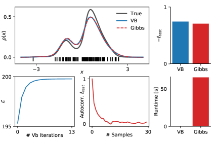
Figure 1: 1D data from the generative model. Data consist of $100$ samples from the underlying density sampled from the GP density model. Upper left: True density (black line), data (black vertical bars), mean posterior density inferred by Gibbs sampler (red dashed line) and VB algorithm (blue line). Upper right: Negative log expected test likelihood of Gibbs and VB inferred posterior. Lower left: Variational lower bound as function of iterations of the VB algorithm. Lower middle: Autocorrelation of test likelihood as function of Markov chain samples obtained from Gibbs sampler. Lower right: Runtime of the two algorithms (VB took $0.3\ {\rm s}$).

In Fig. 1 we see a 1 dimensional example dataset, where both inference algorithms recover well the structure of the underlying density. The inferred posterior means are barely distinguishable. However, evaluating the inferred densities on an unseen test set, we note that the Gibbs sampler performs slightly better. Of course, this is expected since the sampler provides exact inference for the generative model and should (on average) not be outperformed by the approximate VB as long as the sampled Markov chain is long enough. In Fig. 1 (bottom left) we see that only $13$ iterations of the VB are required to meet the convergence criterion. For Markov chain samplers to be efficient, correlations between samples should decay quickly. Fig. 1 (bottom middle) shows the autocorrelation of $\ell_{\rm test}$, which was evaluated at each sample of the Markov chain. After about $10$ samples the correlations reach a plateau close to $0$, demonstrating excellent mixing properties of the sampler. Comparing the run time of both algorithms, VB ($0.3\ {\rm s}$) outperforms the sampler $\sim 1\ {\rm min}$ by more than $2$ orders of magnitude.

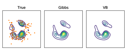
Figure 2: 2D data from generative model. Right: $200$ samples from the underlying two dimensional density. Middle: Posterior mean of Gibbs sampler inferred density. Right: Posterior mean of VB inferred density.

To demonstrate the inference for more complicated problems, $2$ dimensional data are generated with $200$ samples (Fig. 2). The posterior mean densities inferred by both algorithms capture the structure well. As before, the log expected test likelihood is larger for the Gibbs sampler ($\ell_{\rm test}=-296.2$) compared to VB ($\ell_{\rm test}=-306.0$). However, the Gibbs sampler took $>20\ {\rm min}$ while the VB required only $1.8\ \rm{s}$ to obtain the result.

Dim	# points	Gibbs		VB
		$\ell_{\rm test}$	$T$ [s]	$\ell_{\rm test}$	$T$ [s]
1	50	-146.9	30.1	-149.2	1.13
2	100	-257.0	649.9	-260.2	2.03
2	200	-285.3	546.1	-289.6	1.41
6	400	-823.9	4667	-822.2	0.89

Table 1: Performance of Gibbs sampler and VB on different datasets sampled from generative model. $\ell_{\rm test}$ was evaluated on a unknown test set including $50$ samples. In addition, runtime $T$ is reported in seconds.

In Tab. 1 we show results for datasets with different size and different dimensionality. The results confirm that the run time for the Gibbs sampler scales strongly with size and dimensionality of a problem, while the VB algorithm seems relatively unaffected in this regard. However, the VB is in general outperformed by the sampler in terms of expected test likelihood or in the same range. Note, that the runtime of the Gibbs sampler does not solely depend on the number of observed data points $N$ (compare data set 2 and 3 in Tab. 1). As discussed earlier this can happen, when the base measure $\pi(\boldsymbol{x})$ is very different from the target density $\rho(\boldsymbol{x})$ resulting in many latent Poisson events (i.e. $M$ is large).

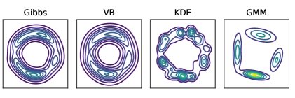
Figure 3: Comparison to other density estimation methods on artificial 2D data. Training data consist of $100$ data points uniformly distributed on a circle ($1.5$ radius) and additional Gaussian noise ($0.2$ std.). From left to right: The posterior mean inferred by Gibbs sampler and VB algorithm, followed by density estimation using KDE and GMM.

	Gibbs	VB	KDE	GMM
$\ell_{\rm test}$	-220.31	-230.53	-228.43	-237.34

Table 2: Log expected test likelihood for circle data.

Circle data

In the following, we compare the GP density model and its two inference algorithms with two alternative density estimation methods. These are given by a kernel density estimator (KDE) with a Gaussian kernel and a Gaussian mixture model (GMM) [25]. The free parameters of these models (kernel bandwidth for KDE and number of components for GMM) are optimised by $10$-fold cross–validation. Furthermore, GMM is initialised $10$ times and the best result is reported. For the GP density model a Gaussian density is assumed as base measure $\pi(\boldsymbol{x})$, and hyperparameters $\boldsymbol{\theta}_{\pi},\ \boldsymbol{\theta}_{k}$, and $\mu_{0}$ are now optimised. Similar to [7] we consider $100$ samples uniformly drawn from a circle with additional Gaussian noise. The inferred densities (only the mean of the posterior for Gibbs and VB) are shown in Fig. 3. Both GP density methods recover well the structure of the data, but the VB seems to overestimate the width of the Gaussian noise compared to the Gibbs sampler. While the KDE also recovers relatively well the data structure the GMM fails in this case. This is also reflected on the log expected test likelihoods (Tab. 2).

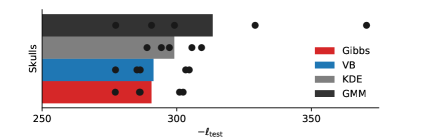
Figure 4: Performance on ‘Egyptian Skulls’ dataset [26]. $100$ training points and $4$ dimensions. Bar height shows average negative log test likelihood obtained by five random permutations of training and test set and points mark single permutation results.

Real data sets

The ‘Egyptian Skulls’ dataset [26] contains $150$ data points in $4$ dimensions. $100$ training points are randomly selected and performance is evaluated on the remaining ones. Before fitting data is whitened. Base measure and fitting procedure for all algorithms are the same as for the circular data. Furthermore, fitting is done for $5$ random permutations of training and test set. The results in Fig. 4 show that both algorithms for the GP density model outperform the two other ones on this dataset.

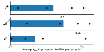
Figure 5: Application on higher dimensional data with many data points. The improvement on log expected test likelihood $\ell_{\rm test}$ per test point compared to GMM, when using same as base measure $\pi(\boldsymbol{x})$ for the VB inference. From top to bottom: ‘Forest Fire’ dataset  [27, 28] ($400$ training points, $117$ test points, $5$ dim.), ‘Thyroid’ dataset [29] ($3\times 10^{3}$, $772$, $6$), ‘Wine’ dataset [27] ($6\times 10^{3}$, $498$, $9$). Bars mark improvement on average of random permutations of training and test set while points mark single runs.

Often practical problems may consist of many more data points and dimensions. As discussed, the Gibbs sampler is not practical for such kind of problems, while the VB could handle larger amounts of data. Unfortunately, the sparsity assumption and the integration via importance sampling is expected to become poorer with increasing number of dimensions. Noting, however, that the ‘effective’ dimensionality in our model is determined by the base measure $\pi(\boldsymbol{x})$, one can circumvent this problem by an educated choice of $\pi(\boldsymbol{x})$ if data ${\cal D}$ lie in a submanifold of the high dimensional space $\mathcal{X}$.

We employ this strategy by first fitting a GMM to the problem and then utilising the fit as base measure. In Fig. 5 we consider $3$ different datasets to test this procedure. As in Fig. 4, fitting is repeated $5$ times for random permutations if training and test set. For the ‘Thyroid’ dataset, one of the $5$ fits is excluded, because the importance sampling yielded poor approximation ${\rm std}(I)>I\times 10^{-2}$. The training sets contain $400$ to $6000$ data points with $5$ to $9$ dimensions. The results for KDE are not reported, since it is always outperformed by the GMM. Fig. 5 demonstrates combining the GMM and VB algorithm results in an improvement of the log test likelihood $\ell_{\rm test}$ compared to using only GMM. Average relative improvements of $\ell_{\rm test}$ are $8.9\ \%$ for ‘Forest Fire’, $4.1\ \%$ for ‘Thyroid’, and $1.1\ \%$ for ‘Wine’ dataset.

5 DISCUSSION

We have shown how inference for a nonparametric, GP based, density model can be made efficient. In the following we would like to discuss various possible extensions but also limitations of our approach.

Choice of base measure

As we have shown for applications to real data, the choice of the base measure is quite important, especially for the sampler and for high dimensional problems. While many datasets might favour a normal distribution as base measure, problems with outliers might favour fat tailed densities. In general, any density which can be evaluated on the data space $\mathcal{X}$ and which allows for efficient sampling, is a valid choice as base measure $\pi(\boldsymbol{x})$ in our inference approach for the GP density model. Any powerful density estimator which fulfils this condition could provide a base measure which could then potentially be improved by the GP model. It would e.g. be interesting to apply this idea to neural networks [30, 31] based estimators. Other generalisations of our model could consider alternative data spaces $\mathcal{X}$. One might e.g. think of specific discrete and structured sets $\mathcal{X}$ for which appropriate Gaussian processes could be defined by suitable Mercer kernels.

Big data & high dimensionality

Our proposed Gibbs sampler suffers from cubic scaling in the number of data points and is found to be already impractical for problems with hundreds of observations. This could potentially be tackled by using sparse (approximate) GP methods for the sampler (see [32] for a potential approach). On the other hand, the proposed VB algorithm scales only linearly with the training set size and can be applied to problems with several thousands of observations. The integration of stochastic variational inference into our method could potentially increase this limit [33].

Potential limitations of the GP density model are given by high dimensional problems. If approached naively, the combination of the sparse GP approximation and the numerical integration using importance sampling is expected to yield bad approximations in such cases. If the data is concentrated on a low dimensional submanifold of the high–dimensional space, one could still try to combine our method with other density estimators providing a base measure $\pi(\boldsymbol{x})$ that is adapted to this submanifold, to allow for tractable GP inference.

Acknowledgements

CD was supported by the Deutsche Forschungsgemeinschaft (GRK1589/2) and partially funded by Deutsche Forschungsgemeinschaft (DFG) through grant CRC 1294 “Data Assimilation”, Project (A06) “Approximative Bayesian inference and model selection for stochastic differential equations (SDEs)”.

Appendix A THE CONDITIONAL POSTERIOR POINT PROCESS

Here we prove that the conditional posterior point process in Equation (17) again is a Poisson process using Campbell’s theorem [11, chap. 3]. For an arbitrary function $h(\cdot,\cdot)$ we set $H\doteq\sum_{(\boldsymbol{x},\omega)\in\Pi}h(\boldsymbol{x},\omega)$. We calculate the characteristic functional

$$\begin{split}&\mathbb{E}_{\phi_{\lambda}}\left[\left.e^{H}\right|g,\lambda\right]=\\ &\frac{\mathbb{E}_{\phi_{\lambda}}\left[\left.\prod_{(\omega,\boldsymbol{x})\in\Pi}e^{f(\omega,-g(\boldsymbol{x}))+h(\boldsymbol{x},\omega)}\right|g,\lambda\right]}{\exp\left(\int_{\mathcal{X}\times\mathbb{R}^{+}}\left(e^{f(\omega,-g(\boldsymbol{x}))}-1\right)\phi_{\lambda}(\boldsymbol{x},\omega)d\omega d\boldsymbol{x}\right)}=\\ &\frac{\exp\left\{\int_{\mathcal{X}\times\mathbb{R}^{+}}\left(e^{f(\omega,-g(\boldsymbol{x}))+h(\boldsymbol{x},\omega)}-1\right)\phi_{\lambda}(\boldsymbol{x},\omega)d\omega d\boldsymbol{x}\right\}}{\exp\left(\int_{\mathcal{X}\times\mathbb{R}^{+}}\left(e^{f(\omega,-g(\boldsymbol{x}))}-1\right)\phi_{\lambda}(\boldsymbol{x},\omega)d\omega d\boldsymbol{x}\right)}=\\ &\exp\left\{\int_{\mathcal{X}\times\mathbb{R}^{+}}\left(e^{h(\boldsymbol{x},\omega)}-1\right)e^{f(\omega,-g)}\phi_{\lambda}(\boldsymbol{x},\omega)d\omega d\boldsymbol{x}\right\}=\\ &\exp\left\{\int_{\mathcal{X}\times\mathbb{R}^{+}}\left(e^{h(\boldsymbol{x},\omega)}-1\right)\Lambda(\boldsymbol{x},\omega)d\omega d\boldsymbol{x}\right\},\end{split}$$ (41)

where the last equality follows from the definition of $\phi_{\lambda}(\boldsymbol{x},\omega)$ and the tilted Polya–Gamma density. Using the fact that a Poisson process is uniquely characterised by its generating function this shows that the conditional posterior $p(\Pi|g,\lambda)$ is a marked Poisson process.

Appendix B VARIATIONAL LOWER BOUND

The full variational lower bound is given by

$$\begin{split}\mathcal{L}(q)=&\sum_{n=1}^{N}\left\{\mathbb{E}_{Q}\left[\ln\lambda\right]+\ln\pi(\boldsymbol{x}_{n})+\mathbb{E}_{Q}\left[f(\omega_{n},g(\boldsymbol{x}_{n}))\right]\right.\\ &\left.-\ln\cosh\left(\frac{c_{n}}{2}\right)+\frac{c_{n}^{2}}{2}\mathbb{E}_{Q}\left[\omega_{n}\right]\right\}\\ &+\int_{\mathcal{X}}\int_{\mathbb{R}^{+}}\left\{\mathbb{E}_{Q}\left[\ln\lambda\right]+\mathbb{E}_{Q}\left[f(\omega,-g(\boldsymbol{x}))\right]-\ln\lambda_{1}\right.\\ &\left.-\ln\sigma(-c(\boldsymbol{x}))-\ln\cosh\left(\frac{c(\boldsymbol{x})}{2}\right)-\frac{c(\boldsymbol{x})^{2}}{2}\omega\right.\\ &\left.-\frac{c(\boldsymbol{x})-g_{1}(\boldsymbol{x})}{2}+1\right\}\Lambda_{1}(\boldsymbol{x},\omega)d\omega d\boldsymbol{x}\\ &-\mathbb{E}_{Q}\left[\lambda\right]+\mathbb{E}_{Q}\left[\ln\frac{p(\lambda)}{q(\lambda)}\right]+\mathbb{E}_{Q}\left[\ln\frac{p(\boldsymbol{g}_{s})}{q(\boldsymbol{g}_{s})}\right].\end{split}$$ (42)

References

- [1] Carl Edward Rasmussen and Christopher KI Williams. Gaussian processes for machine learning, volume 1. MIT press Cambridge, 2006.
- [2] Christopher KI Williams and Carl Edward Rasmussen. Gaussian processes for regression. In Advances in neural information processing systems, pages 514–520, 1996.
- [3] Hannes Nickisch and Carl Edward Rasmussen. Approximations for binary gaussian process classification. Journal of Machine Learning Research, 9(Oct):2035–2078, 2008.
- [4] Ryan Prescott Adams, Iain Murray, and David JC MacKay. Tractable nonparametric bayesian inference in poisson processes with gaussian process intensities. In Proceedings of the 26th Annual International Conference on Machine Learning, pages 9–16. ACM, 2009.
- [5] Cedric Archambeau, Dan Cornford, Manfred Opper, and John Shawe-Taylor. Gaussian process approximations of stochastic differential equations. In Gaussian Processes in Practice, pages 1–16, 2007.
- [6] Andreas Damianou, Michalis K Titsias, and Neil D Lawrence. Variational gaussian process dynamical systems. In Advances in Neural Information Processing Systems, pages 2510–2518, 2011.
- [7] Iain Murray, David MacKay, and Ryan P Adams. The gaussian process density sampler. In Advances in Neural Information Processing Systems, pages 9–16, 2009.
- [8] Jaakko Riihimäki, Aki Vehtari, et al. Laplace approximation for logistic gaussian process density estimation and regression. Bayesian analysis, 9(2):425–448, 2014.
- [9] Nicholas G Polson, James G Scott, and Jesse Windle. Bayesian inference for logistic models using pólya–gamma latent variables. Journal of the American statistical Association, 108(504):1339–1349, 2013.
- [10] Stephen G Walker. Posterior sampling when the normalizing constant is unknown. Communications in Statistics—Simulation and Computation®, 40(5):784–792, 2011.
- [11] John Frank Charles Kingman. Poisson processes. Wiley Online Library, 1993.
- [12] Takis Konstantopoulos, Zurab Zerakidze, and Grigol Sokhadze. Radon–Nikodým Theorem, pages 1161–1164. Springer Berlin Heidelberg, Berlin, Heidelberg, 2011.
- [13] Stuart Geman and Donald Geman. Stochastic relaxation, gibbs distributions, and the bayesian restoration of images. In Readings in Computer Vision, pages 564–584. Elsevier, 1987.
- [14] Scott Linderman. pypolyagamma. https://github.com/slinderman/pypolyagamma, 2017.
- [15] W Keith Hastings. Monte carlo sampling methods using markov chains and their applications. Biometrika, 57(1):97–109, 1970.
- [16] Christopher M Bishop. Pattern recognition and machine learning. springer, 2006.
- [17] Lehel Csató. Gaussian Processes -Iterative Sparse Approximations. PhD Thesis, 2002.
- [18] Lehel Csató, Manfred Opper, and Ole Winther. Tap gibbs free energy, belief propagation and sparsity. In T. G. Dietterich, S. Becker, and Z. Ghahramani, editors, Advances in Neural Information Processing Systems 14, pages 657–663. MIT Press, 2002.
- [19] Michalis K Titsias. Variational learning of inducing variables in sparse gaussian processes. In International Conference on Artificial Intelligence and Statistics, pages 567–574, 2009.
- [20] Edward Snelson and Zoubin Ghahramani. Sparse gaussian processes using pseudo-inputs. In Advances in neural information processing systems, pages 1257–1264, 2006.
- [21] Alexander G de G Matthews, James Hensman, Richard Turner, and Zoubin Ghahramani. On sparse variational methods and the kullback-leibler divergence between stochastic processes. In Artificial Intelligence and Statistics, pages 231–239, 2016.
- [22] Philipp Batz, Andreas Ruttor, and Manfred Opper. Approximate bayes learning of stochastic differential equations. arXiv preprint arXiv:1702.05390, 2017.
- [23] Diederik P Kingma and Jimmy Ba. Adam: A method for stochastic optimization. arXiv preprint arXiv:1412.6980, 2014.
- [24] Christian Donner. Sgpd_inference. https://github.com/christiando/SGPD_Inference, 2018.
- [25] F. Pedregosa, G. Varoquaux, A. Gramfort, V. Michel, B. Thirion, O. Grisel, M. Blondel, P. Prettenhofer, R. Weiss, V. Dubourg, J. Vanderplas, A. Passos, D. Cournapeau, M. Brucher, M. Perrot, and E. Duchesnay. Scikit-learn: Machine Learning in Python . Journal of Machine Learning Research, 12:2825–2830, 2011.
- [26] David J Hand, Fergus Daly, K McConway, D Lunn, and E Ostrowski. A handbook of small data sets, volume 1. cRc Press, 1993.
- [27] Dua Dheeru and Efi Karra Taniskidou. UCI machine learning repository, 2017.
- [28] Paulo Cortez and Aníbal de Jesus Raimundo Morais. A data mining approach to predict forest fires using meteorological data. 2007.
- [29] Fabian Keller, Emmanuel Muller, and Klemens Bohm. Hics: high contrast subspaces for density-based outlier ranking. In Data Engineering (ICDE), 2012 IEEE 28th International Conference on, pages 1037–1048. IEEE, 2012.
- [30] Hugo Larochelle and Iain Murray. The neural autoregressive distribution estimator. In Proceedings of the Fourteenth International Conference on Artificial Intelligence and Statistics, pages 29–37, 2011.
- [31] Benigno Uria, Iain Murray, and Hugo Larochelle. A deep and tractable density estimator. In International Conference on Machine Learning, pages 467–475, 2014.
- [32] Yves-Laurent Kom Samo and Stephen Roberts. Scalable nonparametric bayesian inference on point processes with gaussian processes. In International Conference on Machine Learning, pages 2227–2236, 2015.
- [33] Matthew D Hoffman, David M Blei, Chong Wang, and John Paisley. Stochastic variational inference. The Journal of Machine Learning Research, 14(1):1303–1347, 2013.
- [34] Yarin Gal and Richard Turner. Improving the gaussian process sparse spectrum approximation by representing uncertainty in frequency inputs. In International Conference on Machine Learning, pages 655–664, 2015.