AMR Dependency Parsing with a Typed Semantic Algebra

Abstract

We present a semantic parser for Abstract Meaning Representations which learns to parse strings into tree representations of the compositional structure of an AMR graph. This allows us to use standard neural techniques for supertagging and dependency tree parsing, constrained by a linguistically principled type system. We present two approximative decoding algorithms, which achieve state-of-the-art accuracy and outperform strong baselines.

1 Introduction

Over the past few years, Abstract Meaning Representations (AMRs, Banarescu et al. (2013)) have become a popular target representation for semantic parsing. AMRs are graphs which describe the predicate-argument structure of a sentence. Because they are graphs and not trees, they can capture reentrant semantic relations, such as those induced by control verbs and coordination. However, it is technically much more challenging to parse a string into a graph than into a tree. For instance, grammar-based approaches Peng et al. (2015); Artzi et al. (2015) require the induction of a grammar from the training corpus, which is hard because graphs can be decomposed into smaller pieces in far more ways than trees. Neural sequence-to-sequence models, which do very well on string-to-tree parsing Vinyals et al. (2014), can be applied to AMRs but face the challenge that graphs cannot easily be represented as sequences van Noord and Bos (2017a, b).

In this paper, we tackle this challenge by making the compositional structure of the AMR explicit. As in our previous work, Groschwitz et al. (2017), we view an AMR as consisting of atomic graphs representing the meanings of the individual words, which were combined compositionally using linguistically motivated operations for combining a head with its arguments and modifiers. We represent this structure as terms over the AM algebra as defined in Groschwitz et al. (2017). This previous work had no parser; here we show that the terms of the AM algebra can be viewed as dependency trees over the string, and we train a dependency parser to map strings into such trees, which we then evaluate into AMRs in a postprocessing step. The dependency parser relies on type information, which encodes the semantic valencies of the atomic graphs, to guide its decisions.

More specifically, we combine a neural supertagger for identifying the elementary graphs for the individual words with a neural dependency model along the lines of Kiperwasser and Goldberg (2016) for identifying the operations of the algebra. One key challenge is that the resulting term of the AM algebra must be semantically well-typed. This makes the decoding problem NP-complete. We present two approximation algorithms: one which takes the unlabeled dependency tree as given, and one which assumes that all dependencies are projective. We evaluate on two data sets, achieving state-of-the-art results on one and near state-of-the-art results on the other (Smatch f-scores of 71.0 and 70.2 respectively). Our approach clearly outperforms strong but non-compositional baselines.

Plan of the paper. After reviewing related work in Section 2, we explain the AM algebra in Section 3 and extend it to a dependency view in Section 4. We explain model training in Section 5 and decoding in Section 6. Section 7 evaluates a number of variants of our system.

2 Related Work

Recently, AMR parsing has generated considerable research activity, due to the availability of large-scale annotated data Banarescu et al. (2013) and two successful SemEval Challenges May (2016); May and Priyadarshi (2017).

Methods from dependency parsing have been shown to be very successful for AMR parsing. For instance, the JAMR parser Flanigan et al. (2014, 2016) distinguishes concept identification (assigning graph fragments to words) from relation identification (adding graph edges which connect these fragments), and solves the former with a supertagging-style method and the latter with a graph-based dependency parser. Foland and Martin (2017) use a variant of this method based on an intricate neural model, yielding state-of-the-art results. We go beyond these approaches by explicitly modeling the compositional structure of the AMR, which allows the dependency parser to combine AMRs for the words using a small set of universal operations, guided by the types of these AMRs.

Other recent methods directly implement a dependency parser for AMRs, e.g. the transition-based model of Damonte et al. (2017), or postprocess the output of a dependency parser by adding missing edges Du et al. (2014); Wang et al. (2015). In contrast to these, our model makes no strong assumptions on the dependency parsing algorithm that is used; here we choose that of Kiperwasser and Goldberg (2016).

The commitment of our parser to derive AMRs compositionally mirrors that of grammar-based AMR parsers Artzi et al. (2015); Peng et al. (2015). In particular, there are parallels between the types we use in the AM algebra and CCG categories (see Section 3 for details). As a neural system, our parser struggles less with coverage issues than these, and avoids the complex grammar induction process these models require.

More generally, our use of semantic types to restrict our parser is reminiscent of Kwiatkowski et al. (2010), Krishnamurthy et al. (2017) and Zhang et al. (2017), and the idea of deriving semantic representations from dependency trees is also present in Reddy et al. (2017).

3 The AM algebra

A core idea of this paper is to parse a string into a graph by instead parsing a string into a dependency-style tree representation of the graph’s compositional structure, represented as terms of the Apply-Modify (AM) algebra Groschwitz et al. (2017).

The values of the AM algebra are annotated s-graphs, or as-graphs: directed graphs with node and edge labels in which certain nodes have been designated as sources Courcelle and Engelfriet (2012) and annotated with type information. Some examples of as-graphs are shown in Fig. 1. Each as-graph has exactly one root, indicated by the bold outline. The sources are indicated by red labels; for instance, $G_{\text{want}}$ has an s-source and an o-source. The annotations, written in square brackets behind the red source names, will be explained below. We use these sources to mark open argument slots; for example, $G_{\text{sleep}}$ in Fig. 1 represents an intransitive verb, missing its subject, which will be added at the s-source.

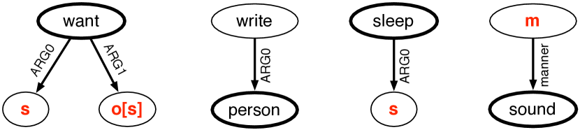
Figure 1: Elementary as-graphs $G_{\text{want}}$, $G_{\text{writer}}$, $G_{\text{sleep}}$, and $G_{\text{sound}}$ for the words “want”, “writer”, “sleep”, and “soundly” respectively.

The AM algebra can combine as-graphs with each other using two linguistically motivated operations: apply and modify. Apply (App) adds an argument to a predicate. For example, we can add a subject – the graph $G_{\text{writer}}$ in Fig. 1 – to the graph $G_{\text{VP }}$in Fig. 2d using App${}_{\text{\text{{s}}}}$, yielding the complete AMR in Fig. 2b. Linguistically, this is like filling the subject (s) slot of the predicate wants to sleep soundly with the argument the writer. In general, for a source $a$, $\text{{App}}_{a}(G_{P},G_{A})$, combines the as-graph $G_{P}$ representing a predicate, or head, with the as-graph $G_{A}$, which represents an argument. It does this by plugging the root node of $G_{A}$ into the $a$-source $u$ of $G_{P}$ – that is, the node $u$ of $G_{P}$ marked with source $a$. The root of the resulting as-graph $G$ is the root of $G_{P}$, and we remove the $a$ marking on $u$, since that slot is now filled.

The modify operation (Mod) adds a modifier to a graph. For example, we can combine two elementary graphs from Fig. 1 with Mod_m ($G_{\text{sleep}}$, $G_{\text{sound}}$), yielding the graph in Fig. 2c. The m-source of the modifier $G_{\text{soundly}}$ attaches to the root of $G_{\text{sleep}}$. The root of the result is the same as the root of $G_{\text{sleep}}$ in the same sense that a verb phrase with an adverb modifier is still a verb phrase. In general, $\text{{Mod}}_{a}(G_{H},G_{M})$, combines a head $G_{H}$ with a modifier $G_{M}$. It plugs the root of $G_{H}$ into the $a$-source $u$ of $G_{M}$. Although this may add incoming edges to the root of $G_{H}$, that node is still the root of the resulting graph $G$. We remove the $a$ marking from $G_{M}$.

In both App and Mod, if there is any other source $b$ which is present in both graphs, the nodes marked with $b$ are unified with each other. For example, when $G_{\text{want}}$ is o-applied to $t_{1}$ in Fig. 2d, the s-sources of the graphs for “want” and “sleep soundly” are unified into a single node, creating a reentrancy. This falls out of the definition of merge for s-graphs which formally underlies both operations (see Courcelle and Engelfriet (2012)).

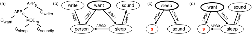
Figure 2: (a) An AM-term with its value (b), along with the values for its subexpressions (c) $t_{1}=\text{{Mod}}_{m}(G_{\text{sleep}},G_{\text{sound}})$ and (d) $t_{2}=\text{{App}}_{o}(G_{\text{want}},t_{1})$.

Finally, the AM algebra uses types to restrict its operations. Here we define the type of an as-graph as the set of its sources with their annotations; thus for example, in Fig. 1, the graph for “writer” has the empty type $[\;]$, $G_{\text{sleep}}$ has type $[\text{\text{{s}}}]$, and $G_{\text{want}}$ has type $[\text{\text{{s}}},\text{\text{{o}}}{[\text{\text{{s}}}]}]$. Each source in an as-graph specifies with its annotation the type of the as-graph which is plugged into it via App. In other words, for a source $a$, we may only $a$-apply $G_{P}$ with $G_{A}$ if the annotation of the $a$-source in $G_{P}$ matches the type of $G_{A}$. For example, the o-source of $G_{\text{wants}}$ (Fig. 1) requires that we plug in an as-graph of type $[\text{{s}}]$; observe that this means that the reentrancy in Fig. 2b is lexically specified by the control verb “want”. All other source nodes in Fig. 1 have no annotation, indicating a type requirement of $[\;]$.

Linguistically, modification is optional; we therefore want the modified graph to be derivationally just like the unmodified graph, in that exactly the same operations can apply to it. In a typed algebra, this means Mod should not change the type of the head. Mod_a therefore requires that the modifier $G_{M}$ have no sources not already present in the head $G_{H}$, except $a$, which will be deleted anyway.

As in any algebra, we can build terms from constants (denoting elementary as-graphs) by recursively combining them with the operations of the AM algebra. By evaluating the operations bottom-up, we obtain an as-graph as the value of such a term; see Fig. 2 for an example. However, as discussed above, an operation in the term may be undefined due to a type mismatch. We call an AM-term well-typed if all its operations are defined. Every well-typed AM-term evaluates to an as-graph. Since the applicability of an AM operation depends only on the types, we also write $\tau=\text{{f}}(\tau_{1},\tau_{2})$ if as-graphs of type $\tau_{1}$ and $\tau_{2}$ can be combined with the operation f and the result has type $\tau$.

Relationship to CCG.

There is close relationship between the types of the AM algebra and the categories of CCG. A type $[\text{{s}},\text{{o}}]$ specifies that the as-graph needs to be applied to two arguments to be semantically complete, similar a CCG category such as $\mathrm{S}\backslash\mathrm{NP}/\mathrm{NP}$, where a string needs to be applied to two NP arguments to be syntactically complete. However, AM types govern the combination of graphs, while CCG categories control the combination of strings. This relieves AM types of the need to talk about word order; there are no “forward” or “backward” slashes in AM types, and a smaller set of operations. Also, the AM algebra spells out raising and control phenomena more explicitly in the types.

4 Indexed AM terms

In this paper, we connect AM terms to the input string $w$ for which we want to produce a graph. We do this in an indexed AM term, exemplified in Fig. 3a. We assume that every elementary as-graph $G$ at a leaf represents the meaning of an individual word token $w_{i}$ in $w$, and write $G[i]$ to annotate the leaf $G$ with the index $i$ of this token. This induces a connection between the nodes of the AMR and the tokens of the string, in that the label of each node was contributed by the elementary as-graph of exactly one token.

We define the head index of a subtree $t$ to be the index of the token which contributed the root of the as-graph to which $t$ evaluates. For a leaf with annotation $i$, the head index is $i$; for an App or Mod node, the head index is the head index of the left child, i.e. of the head argument. We annotate each App and Mod operation with the head index of the left and right subtree.

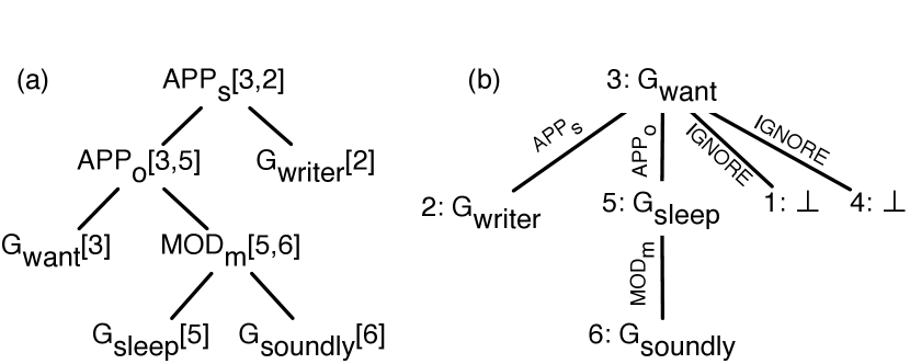
Figure 3: (a) An indexed AM term and (b) an AM dependency tree, linking the term in Fig. 2;a to the sentence “The writer wants to sleep soundly”.

4.1 AM dependency trees

We can represent indexed AM terms more compactly as AM dependency trees, as shown in Fig. 3b. The nodes of such a dependency tree are the tokens of $w$. We draw an edge with label f from $i$ to $k$ if there is a node with label $\text{{f}}[i,k]$ in the indexed AM term. For example, the tree in 3b has an edge labeled Mod_m from 5 ($G_{\text{sleep}}$) to 6 ($G_{\text{soundly}}$) because there is a node in the term in 3a labeled $\text{{Mod}}_{m}[5,6]$. The same AM dependency tree may represent multiple indexed AM terms, because the order of apply and modify operations is not specified in the dependency tree. However, it can be shown that all well-typed AM terms that map to the same AM dependency tree evaluate to the same as-graph. We define a well-typed AM dependency tree as one that represents a well-typed AM term.

Because not all words in the sentence contribute to the AMR, we include a mechanism for ignoring words in the input. As a special case, we allow the constant $\bot$, which represents a dummy as-graph (of type $\bot$) which we use as the semantic value of words without a semantic value in the AMR. We furthermore allow the edge label ignore in an AM dependency tree, where $\text{{ignore}}(\tau_{1},\tau_{2})=\tau_{1}$ if $\tau_{2}=\bot$ and is undefined otherwise; in particular, an AM dependency tree with ignore edges is only well-typed if all ignore edges point into $\bot$ nodes. We keep all other operations $\text{{f}}(\tau_{1},\tau_{2})$ as is, i.e. they are undefined if either $\tau_{1}$ or $\tau_{2}$ is $\bot$, and never yield $\bot$ as a result. When reconstructing an AM term from the AM dependency tree, we skip ignore edges, such that the subtree below them will not contribute to the overall AMR.

4.2 Converting AMRs to AM terms

In order to train a model that parses sentences into AM dependency trees, we need to convert an AMR corpus – in which sentences are annotated with AMRs – into a treebank of AM dependency trees. We do this in three steps: first, we break each AMR up into elementary graphs and identify their roots; second, we assign sources and annotations to make elementary as-graphs out of them; and third, combine them into indexed AM terms.

For the first step, an aligner uses hand-written heuristics to identify the string token to which each node in the AMR corresponds (see Section C in the Supplementary Materials for details). We proceed in a similar fashion as the JAMR aligner Flanigan et al. (2014), i.e. by starting from high-confidence token-node pairs and then extending them until the whole AMR is covered. Unlike the JAMR aligner, our heuristics ensure that exactly one node in each elementary graph is marked as the root, i.e. as the node where other graphs can attach their edges through App and Mod. When an edge connects nodes of two different elementary graphs, we use the “blob decomposition” algorithm of Groschwitz et al. (2017) to decide to which elementary graph it belongs. For the example AMR in Fig. 2b, we would obtain the graphs in Fig. 1 (without source annotations). Note that ARG edges belong with the nodes at which they start, whereas the “manner” edge in $G_{\text{soundly}}$ goes with its target.

In the second step we assign source names and annotations to the unlabeled nodes of each elementary graph. Note that the annotations are crucial to our system’s ability to generate graphs with reentrancies. We mostly follow the algorithm of Groschwitz et al. (2017), which determines necessary annotations based on the structure of the given graph. The algorithm chooses each source name depending on the incoming edge label. For instance, the two leaves of $G_{\text{want}}$ can have the source labels s and o because they have incoming edges labeled ARG0 and ARG1. However, the Groschwitz algorithm is not deterministic: It allows object promotion (the sources for an ARG3 edge may be o3, o2, or o), unaccusative subjects (promoting the minimal object to s if the elementary graph contains an ARGi-edge ($i>0$) but no ARG0-edge Perlmutter (1978)), and passive alternation (swapping o and s). To make our as-graphs more consistent, we prefer constants that promote objects as far as possible, use unaccusative subjects, and no passive alternation, but still allow constants that do not satisfy these conditions if necessary. This increased our Smatch score significantly.

Finally, we choose an arbitrary AM dependency tree that combines the chosen elementary as-graphs into the annotated AMR; in practice, the differences between the trees seem to be negligible.

5 Training

We can now model the AMR parsing task as the problem of computing the best well-typed AM dependency tree $t$ for a given sentence $w$. Because $t$ is well-typed, it can be decoded into an (indexed) AM term and thence evaluated to an as-graph.

We describe $t$ in terms of the elementary as-graphs $G[i]$ it uses for each token $i$ and of its edges $\text{{f}}[i,k]$. We assume a node-factored, edge-factored model for the score $\omega(t)$ of $t$:

$$\omega(t)=\sum_{1\leq i\leq n}\omega(G[i])+\sum_{\text{{f}}[i,k]\in E}\omega(\text{{f}}[i,k]),$$ (1)

where the edge weight further decomposes into the sum $\omega(\text{{f}}[i,k])=\omega(i\rightarrow k)+\omega(\text{{f}}\mid i\rightarrow k)$ of a score $\omega(i\rightarrow k)$ for the presence of an edge from $i$ to $k$ and a score $\omega(\text{{f}}\mid i\rightarrow k)$ for this edge having label f. Our aim is to compute the well-typed $t$ with the highest score.

We present three models for $\omega$: one for the graph scores and two for the edge scores. All of these are based on a two-layer bidirectional LSTM, which reads inputs $\mathbf{x}=(x_{1},\ldots,x_{n})$ token by token, concatenating the hidden states of the forward and the backward LSTMs in each layer. On the second layer, we thus obtain vector representations $v_{i}=\mbox{BiLSTM}(\mathbf{x},i)$ for the individual input tokens (see Fig. 4). Our models differ in the inputs $\mathbf{x}$ and the way they predict scores from the $v_{i}$.

5.1 Supertagging for elementary as-graphs

We construe the prediction of the as-graphs $G[i]$ for each input position $i$ as a supertagging task Lewis et al. (2016). The supertagger reads inputs $x_{i}=(w_{i},p_{i},c_{i})$, where $w_{i}$ is the word token, $p_{i}$ its POS tag, and $c_{i}$ is a character-based LSTM encoding of $w_{i}$. We use pretrained GloVe embeddings Pennington et al. (2014) concatenated with learned embeddings for $w_{i}$, and learned embeddings for $p_{i}$.

To predict the score for each elementary as-graph out of a set of $K$ options, we add a $K$-dimensional output layer as follows:

$$\omega(G[i])=\log{\mbox{softmax}}(W\cdot v_{i}+b)$$

and train the neural network using a cross-entropy loss function. This maximizes the likelihood of the elementary as-graphs in the training data.

5.2 Kiperwasser & Goldberg edge model

Predicting the edge scores amounts to a dependency parsing problem. We chose the dependency parser of Kiperwasser and Goldberg (2016), henceforth K&G, to learn them, because of its accuracy and its fit with our overall architecture. The K&G parser scores the potential edge from $i$ to $k$ and its label from the concatenations of $v_{i}$ and $v_{k}$:

$$\begin{array}[]{rcl}\mbox{MLP}_{\theta}(v)&=&W_{2}\cdot\tanh(W_{1}\cdot v+b_{1})+b_{2}\\ \omega(i\rightarrow k)&=&\mbox{MLP}_{\mbox{{e}}}(v_{i}\circ v_{k})\\ \omega(\text{{f}}{}\mid i\rightarrow k)&=&\mbox{MLP}_{\mbox{{lbl}}}(v_{i}\circ v_{k})\end{array}$$

We use inputs $x_{i}=(w_{i},p_{i},\tau_{i})$ including the type $\tau_{i}$ of the supertag $G[i]$ at position $i$, using trained embeddings for all three. At evaluation time, we use the best scoring supertag according to the model of Section 5.1. At training time, we sample from $q$, where $q(\tau_{i})=(1-\delta)+\delta\cdot p(\tau_{i}|p_{i},p_{i-1})$, $q(\tau)=\delta\cdot p(\tau|p_{i},p_{i-1})$ for any $\tau\neq\tau_{i}$ and $\delta$ is a hyperparameter controlling the bias towards the aligned supertag. We train the model using K&G’s original DyNet implementation. Their algorithm uses a hinge loss function, which maximizes the score difference between the gold dependency tree and the best predicted dependency tree, and therefore requires parsing each training instance in each iteration. Because the AM dependency trees are highly non-projective, we replaced the projective parser used in the off-the-shelf implementation by the Chu-Liu-Edmonds algorithm implemented in the TurboParser Martins et al. (2010), improving the LAS on the development set by 30 points.

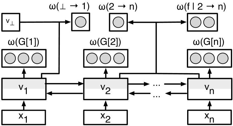
Figure 4: Architecture of the neural taggers.

5.3 Local edge model

We also trained a local edge score model, which uses a cross-entropy rather than a hinge loss and therefore avoids the repeated parsing at training time. Instead, we follow the intuition that every node in a dependency tree has at most one incoming edge, and train the model to score the correct incoming edge as high as possible. This model takes inputs $x_{i}=(w_{i},p_{i})$.

We define the edge and edge label scores as in Section 5.2, with tanh replaced by ReLU. We further add a learned parameter $v_{\bot}$ for the “LSTM embedding” of a nonexistent node, obtaining scores $\omega(\bot\rightarrow k)$ for $k$ having no incoming edge.

To train $\omega(i\rightarrow k)$, we collect all scores for edges ending at the same node $k$ into a vector $\omega(\bullet\rightarrow k)$. We then minimize the cross-entropy loss for the gold edge into $k$ under ${\mbox{softmax}}(\omega(\bullet\rightarrow k))$, maximizing the likelihood of the gold edges. To train the labels $\omega(\text{{f}}\mid i\rightarrow k)$, we simply minimize the cross-entropy loss of the actual edge labels f of the edges which are present in the gold AM dependency trees.

The PyTorch code for this and the supertagger are available at bitbucket.org/tclup/amr-dependency.

6 Decoding

Given learned estimates for the graph and edge scores, we now tackle the challenge of computing the best well-typed dependency tree $t$ for the input string $w$, under the score model (equation (1)). The requirement that $t$ must be well-typed is crucial to ensure that it can be evaluated to an AMR graph, but as we show in the Supplementary Materials (Section A), makes the decoding problem NP-complete. Thus, an exact algorithm is not practical. In this section, we develop two different approximation algorithms for AM dependency parsing: one which assumes the (unlabeled) dependency tree structure as known, and one which assumes that the AM dependency tree is projective.

$\displaystyle\begin{array}[]{@{}c@{}}s=\omega(G[i])\quad G\neq\bot\\ \hline\cr([i,i+1],i,\tau(G)):s\end{array}$   Init

$\displaystyle\begin{array}[]{@{}c@{}}([i,k],r,\tau):s\quad s^{\prime}=\omega(\bot[k])\\ \hline\cr([i,k+1],r,\tau):s+s^{\prime}\end{array}$   Skip-R

$\displaystyle\begin{array}[]{@{}c@{}}([i,k],r,\tau):s\quad s^{\prime}=\omega(\bot[i-1])\\ \hline\cr([i-1,k],r,\tau):s+s^{\prime}\end{array}$   Skip-L

  $([i,j],r_{1},\tau_{1}):s_{1}\quad([j,k],r_{2},\tau_{2}):s_{2}$ $\tau=\text{{f}}(\tau_{1},\tau_{2})\;\mbox{defined}\quad s=\omega(\text{{f}}[r_{1},r_{2}])$    Arc-R [f]                                   $([i,k],r_{1},\tau):s_{1}+s_{2}+s$

  $([i,j],r_{1},\tau_{1}):s_{1}\quad([j,k],r_{2},\tau_{2}):s_{2}$ $\tau=\text{{f}}(\tau_{2},\tau_{1})\;\mbox{defined}\quad s=\omega(\text{{f}}[r_{2},r_{1}])$    Arc-L [f]                                   $([i,k],r_{2},\tau):s_{1}+s_{2}+s$

Figure 5: Rules for the projective decoder.

6.1 Projective decoder

The projective decoder assumes that the AM dependency tree is projective, i.e. has no crossing dependency edges. Because of this assumption, it can recursively combine adjacent substrings using dynamic programming. The algorithm is shown in Fig. 5 as a parsing schema Shieber et al. (1995), which derives items of the form $([i,k],r,\tau)$ with scores $s$. An item represents a well-typed derivation of the substring from $i$ to $k$ with head index $r$, and which evaluates to an as-graph of type $\tau$.

The parsing schema consists of three types of rules. First, the Init rule generates an item for each graph fragment $G[i]$ that the supertagger predicted for the token $w_{i}$, along with the score and type of that graph fragment. Second, given items for adjacent substrings $[i,j]$ and $[j,k]$, the Arc rules apply an operation f to combine the indexed AM terms for the two substrings, with Arc-R making the left-hand substring the head and the right-hand substring the argument or modifier, and Arc-L the other way around. We ensure that the result is well-typed by requiring that the types can be combined with f. Finally, the Skip rules allow us to extend a substring such that it covers tokens which do not correspond to a graph fragment (i.e., their AM term is $\bot$), introducing ignore edges. After all possible items have been derived, we extract the best well-typed tree from the item of the form $([1,n],r,\tau)$ with the highest score, where $\tau=[\;]$.

Because we keep track of the head indices, the projective decoder is a bilexical parsing algorithm, and shares a parsing complexity of $O(n^{5})$ with other bilexical algorithms such as the Collins parser. It could be improved to a complexity of $O(n^{4})$ using the algorithm of Eisner and Satta (1999).

6.2 Fixed-tree decoder

The fixed-tree decoder computes the best unlabeled dependency tree $t_{r}$ for $w$, using the edge scores $\omega(i\rightarrow k)$, and then computes the best AM dependency tree for $w$ whose unlabeled version is $t_{r}$. The Chu-Liu-Edmonds algorithm produces a forest of dependency trees, which we want to combine into $t_{r}$. We choose the tree whose root $r$ has the highest score for being the root of the AM dependency tree and make the roots of all others children of $r$.

$\displaystyle\begin{array}[]{@{}c@{}}s=\omega(G[i])\\ \hline\cr(i,\emptyset,\tau(G)):s\end{array}$   Init

   $(i,C_{1},\tau_{1}):s_{1}\quad(k,Ch(k),\tau_{2}):s_{2}$ $k\in Ch(i)\backslash C_{1}$ $\tau=\text{{f}}(\tau_{1},\tau_{2})\;\mbox{defined}\quad s=\omega(\text{{f}}[i,k])$    Edge[f]                                            $(i,C_{1}\cup\{k\},\tau):s_{1}+s_{2}+s$

Figure 6: Rules for the fixed-tree decoder.

At this point, the shape of $t_{r}$ is fixed. We choose supertags for the nodes and edge labels for the edges by traversing $t_{r}$ bottom-up, computing types for the subtrees as we go along. Formally, we apply the parsing schema in Fig. 6. It uses items of the form $(i,C,\tau):s$, where $1\leq i\leq n$ is a node of $t_{r}$, $C$ is the set of children of $i$ for which we have already chosen edge labels, and $\tau$ is a type. We write $Ch(i)$ for the set of children of $i$ in $t_{r}$.

The Init rule generates an item for each graph that the supertagger can assign to each token $i$ in $w$, ensuring that every token is also assigned $\bot$ as a possible supertag. The Edge rule labels an edge from a parent node $i$ in $t_{r}$ to one of its children $k$, whose children already have edge labels. As above, this rule ensures that a well-typed AM dependency tree is generated by locally checking the types. In particular, if all types $\tau_{2}$ that can be derived for $k$ are incompatible with $\tau_{1}$, we fall back to an item for $k$ with $\tau_{2}=\bot$ (which always exists), along with an ignore edge from $i$ to $k$.

The complexity of this algorithm is $O(n\cdot 2^{d}\cdot d)$, where $d$ is the maximal arity of the nodes in $t_{r}$.

7 Evaluation

We evaluate our models on the LDC2015E86 and LDC2017T10 datasets (henceforth “2015” and “2017”). Technical details and hyperparameters of our implementation can be found in Sections B to D of the Supplementary Materials.

7.1 Training data

The original LDC datasets pair strings with AMRs. We convert each AMR in the training and development set into an AM dependency tree, using the procedure of Section 4.2. About 10% of the training instances cannot be split into elementary as-graphs by our aligner; we removed these from the training data. Of the remaining AM dependency trees, 37% are non-projective.

Furthermore, the AM algebra is designed to handle short-range reentrancies, modeling grammatical phenomena such as control and coordination, as in the derivation in Fig. 2. It cannot easily handle the long-range reentrancies in AMRs which are caused by coreference, a non-compositional phenomenon. We remove such reentrancies from our training data (about 60% of the roughly 20,000 reentrant edges). Despite this, our model performs well on reentrant edges (see Table 2).

7.2 Pre- and postprocessing

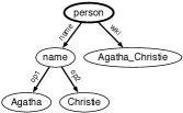
Figure 7: A named entity

We use simple pre- and postprocessing steps to handle rare words and some AMR-specific patterns. In AMRs, named entities follow a pattern shown in Fig. 7. Here the named entity is of type “person”, has a name edge to a “name” node whose children spell out the tokens of “Agatha Christie”, and a link to a wiki entry. Before training, we replace each “name” node, its children, and the corresponding span in the sentence with a special NAME token, and we completely remove wiki edges. In this example, this leaves us with only a “person” and a NAME node. Further, we replace numbers and some date patterns with NUMBER and DATE tokens. On the training data this is straightforward, since names and dates are explicitly annotated in the AMR. At evaluation time, we detect dates and numbers with regular expressions, and names with Stanford CoreNLP Manning et al. (2014). We also use Stanford CoreNLP for our POS tags.

Each elementary as-graph generated by the procedure of Section 4.2 has a unique node whose label corresponds most closely to the aligned word (e.g. the “want” node in $G_{\text{want}}$ and the “write” node in $G_{\text{writer}}$). We replace these node labels with LEX in preprocessing, reducing the number of different elementary as-graphs from 28730 to 2370. We factor the supertagger model of Section 5.1 such that the unlexicalized version of $G[i]$ and the label for LEX are predicted separately.

At evaluation, we re-lexicalize all LEX nodes in the predicted AMR. For words that were frequent in the training data (at least 10 times), we take the supertagger’s prediction for the label. For rarer words, we use simple heuristics, explained in the Supplementary Materials (Section D). For names, we just look up name nodes with their children and wiki entries observed for the name string in the training data, and for unseen names use the literal tokens as the name, and no wiki entry. Similarly, we collect the type for each encountered name (e.g. “person” for “Agatha Christie”), and correct it in the output if the tagger made a different prediction. We recover dates and numbers straightforwardly.

7.3 Supertagger accuracy

All of our models rely on the supertagger to predict elementary as-graphs; they differ only in the edge scores. We evaluated the accuracy of the supertagger on the converted development set (in which each token has a supertag) of the 2015 data set, and achieved an accuracy of 73%. The correct supertag is within the supertagger’s 4 best predictions for 90% of the tokens, and within the 10 best for 95%.

Interestingly, supertags that introduce grammatical reentrancies are predicted quite reliably, although they are relatively rare in the training data. The elementary as-graph for subject control verbs (see $G_{\text{want}}$ in Fig. 1) accounts for only 0.8% of supertags in the training data, yet 58% of its occurrences in the development data are predicted correctly (84% in 4-best). The supertag for VP coordination (with type $[\text{{op1}}[\text{{s}}],\text{{op2}}[\text{{s}}]]$) makes up for 0.4% of the training data, but 74% of its occurrences are recognized correctly (92% in 4-best). Thus the prediction of informative types for individual words is feasible.

7.4 Comparison to Baselines

Type-unaware fixed-tree baseline. The fixed-tree decoder is built to ensure well-typedness of the predicted AM dependency trees. To investigate to what extent this is required, we consider a baseline which just adds the individually highest-scoring supertags and edge labels to the unlabeled dependency tree $t_{u}$, ignoring types. This leads to AM dependency trees which are not well-typed for 75% of the sentences (we fall back to the largest well-typed subtree in these cases). Thus, an off-the-shelf dependency parser can reliably predict the tree structure of the AM dependency tree, but correct supertag and edge label assignment requires a decoder which takes the types into account.

JAMR-style baseline. Our elementary as-graphs differ from the elementary graphs used in JAMR-style algorithms in that they contain explicit source nodes, which restrict the way in which they can be combined with other as-graphs. We investigate the impact of this choice by implementing a strong JAMR-style baseline. We adapt the AMR-to-dependency conversion of Section 4.2 by removing all unlabeled nodes with source names from the elementary graphs. For instance, the graph $G_{\text{want}}$ in Fig. 1 now only consists of a single “want” node. We then aim to directly predict AMR edges between these graphs, using a variant of the local edge scoring model of Section 5.3 which learns scores for each edge in isolation. (The assumption for the original local model, that each node has only one incoming edge, does not apply here.)

When parsing a string, we choose the highest-scoring supertag for each word; there are only 628 different supertags in this setting, and 1-best supertagging accuracy is high at 88%. We then follow the JAMR parsing algorithm by predicting all edges whose score is over a threshold (we found -0.02 to be optimal) and then adding edges until the graph is connected. Because we do not predict which node is the root of the AMR, we evaluated this model as if it always predicted the root correctly, overestimating its score slightly.

Model	2015	2017
Ours
local edge + projective decoder	$70.2\scalebox{0.8}{$\pm 0.3$}$	71.0 $\pm 0.5$
local edge + fixed-tree decoder	$69.4\scalebox{0.8}{$\pm 0.6$}$	$70.2\scalebox{0.8}{$\pm 0.5$}$
K&G  edge + projective decoder	$68.6\scalebox{0.8}{$\pm 0.7$}$	$69.4\scalebox{0.8}{$\pm 0.4$}$
K&G  edge + fixed-tree decoder	$69.6\scalebox{0.8}{$\pm 0.4$}$	$69.9\scalebox{0.8}{$\pm 0.2$}$
Baselines
fixed-tree (type-unaware)	$26.0\scalebox{0.8}{$\pm 0.6$}$	$27.9\scalebox{0.8}{$\pm 0.6$}$
JAMR-style	$66.1$	66.2
Previous work
CAMR Wang et al. (2015)	66.5	-
JAMR Flanigan et al. (2016)	67	-
Damonte et al. (2017)	64	-
van Noord and Bos (2017b)	68.5	71.0
Foland and Martin (2017)	70.7	-
Buys and Blunsom (2017)	-	61.9

Table 1: 2015 & 2017 test set Smatch scores

7.5 Results

	2015					2017
Metric	W’15	F’16	D’17	PD	FTD	vN’17	PD	FTD
Smatch	67	67	64	70	70	71	71	70
Unlabeled	69	69	69	73	73	74	74	74
No WSD	64	68	65	71	70	72	72	70
Named Ent.	75	79	83	79	78	79	78	77
Wikification	0	75	64	71	72	65	71	71
Negations	18	45	48	52	52	62	57	55
Concepts	80	83	83	83	84	82	84	84
Reentrancies	41	42	41	46	44	52	49	46
SRL	60	60	56	63	61	66	64	62

Table 2: Details for the LDC2015E86 and LDC2017T10 test sets

Table 1 shows the Smatch scores (Cai and Knight, 2013) of our models, compared to a selection of previously published results. Our results are averages over 4 runs with $95\%$ confidence intervals (JAMR-style baselines are single runs). On the 2015 dataset, our best models (local + projective, K&G + fixed-tree) outperform all previous work, with the exception of the Foland and Martin (2017) model; on the 2017 set we match state of the art results (though note that van Noord and Bos (2017b) use 100k additional sentences of silver data). The fixed-tree decoder seems to work well with either edge model, but performance of the projective decoder drops with the K&G edge scores. It may be that, while the hinge loss used in the K&G edge scoring model is useful to finding the correct unlabeled dependency tree in the fixed-tree decoder, scores for bad edges – which are never used when computing the hinge loss – are not trained accurately. Thus such edges may be erroneously used by the projective decoder.

As expected, the type-unaware baseline has low recall, due to its inability to produce well-typed trees. The fact that our models outperform the JAMR-style baseline so clearly is an indication that they indeed gain some of their accuracy from the type information in the elementary as-graphs, confirming our hypothesis that an explicit model of the compositional structure of the AMR can help the parser learn an accurate model.

Table 2 analyzes the performance of our two best systems (PD = projective, FTD = fixed-tree) in more detail, using the categories of Damonte et al. (2017), and compares them to Wang’s, Flanigan’s, and Damonte’s AMR parsers on the 2015 set and , and van Noord and Bos (2017b) for the 2017 dataset. (Foland and Martin (2017) did not publish such results.) The good scores we achieve on reentrancy identification, despite removing a large amount of reentrant edges from the training data, indicates that our elementary as-graphs successfully encode phenomena such as control and coordination.

The projective decoder is given 4, and the fixed-tree decoder 6, supertags for each token. We trained the supertagging and edge scoring models of Section 5 separately; joint training did not help. Not sampling the supertag types $\tau_{i}$ during training of the K&G model, removing them from the input, and removing the character-based LSTM encodings $c_{i}$ from the input of the supertagger, all reduced our models’ accuracy.

7.6 Differences between the parsers

Although the Smatch scores for our two best models are close, they sometimes struggle with different sentences. The fixed-tree parser is at the mercy of the fixed tree; the projective parser cannot produce non-projective AM dependency trees. It is remarkable that the projective parser does so well, given the prevalence of non-projective trees in the training data. Looking at its analyses, we find that it frequently manages to find a projective tree which yields an (almost) correct AMR, by choosing supertags with unusual types, and by using modify rather than apply (or vice versa).

8 Conclusion

We presented an AMR parser which applies methods from supertagging and dependency parsing to map a string into a well-typed AM term, which it then evaluates into an AMR. The AM term represents the compositional semantic structure of the AMR explicitly, allowing us to use standard tree-based parsing techniques.

The projective parser currently computes the complete parse chart. In future work, we will speed it up through the use of pruning techniques. We will also look into more principled methods for splitting the AMRs into elementary as-graphs to replace our hand-crafted heuristics. In particular, advanced methods for alignments, as in Lyu and Titov (2018), seem promising. Overcoming the need for heuristics also seems to be a crucial ingredient for applying our method to other semantic representations.

Acknowledgements

We would like to thank the anonymous reviewers for their comments. We thank Stefan Grünewald for his contribution to our PyTorch implementation, and want to acknowledge the inspiration obtained from Nguyen et al. (2017). We also extend our thanks to the organizers and participants of the Oslo CAS Meaning Construction workshop on Universal Dependencies. This work was supported by the DFG grant KO 2916/2-1 and a Macquarie University Research Excellence Scholarship for Jonas Groschwitz.

Appendix A NP-completeness of the decoding problem

We prove NP-completeness for the well-typed decoding problem by reduction from Hamiltonian-Path.

Let $G=(V,E)$ be a directed graph with nodes $V=\{1,\ldots,n\}$ and edges $E\subseteq V\times V$. A Hamiltonian path in $G$ is a sequence $(v_{1},\ldots,v_{n})$ that contains each node of $V$ exactly once, such that $(v_{i},v_{i+1})\in E$ for all $1\leq i\leq n-1$. We assume w.l.o.g. that $v_{n}=n$. Deciding whether $G$ has a Hamiltonian path is NP-complete.

Given $G$, we construct an instance of the decoding problem for the sentence $w=1\ldots n$ as follows. We assume that the first graph fragments shown in Fig. 8a (with node label “i”) is the only graph fragment the supertagger allows for 1, …, $n-1$, and the second one (with node label “f”) is the only graph fragment allowed for $n$. We let $\omega(i\rightarrow k)=1$ if $(i,k)\in E$, and zero otherwise.

Under this construction, every well-typed AM dependency tree for $w$ corresponds to a linear sequence of nodes connected by edges with label $\text{{App}}_{s}$ (see Fig. 8c for an example) More specifically, $n$ is a leaf, and every node except for $n$ has precisely one outgoing $\text{{App}}_{s}$ edge; this is enforced by the well-typedness. Because of the edge scores, the score of such a dependency tree is $n-1$ iff it only uses edges that also exist in $G$; otherwise the score is less than $n-1$. Therefore, we can decide whether $G$ has a Hamiltonian path by running the decoder, i.e. computing the highest-scoring well-typed AM dependency tree $t$ for $w$, and checking whether the score of $t$ is $n-1$.

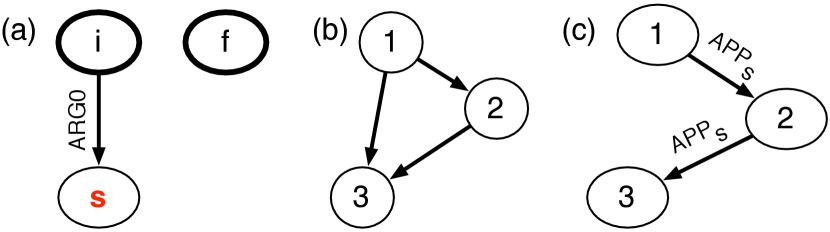
Figure 8: (a) The two graph fragments required for the NP-completeness proof. (b) An example graph and (c) the AM dependency tree corresponding to its Hamiltonian path.

Appendix B Neural Network Details

We implemented the supertagger (Section 5.1) and the local dependency model (Section 5.3) in PyTorch, and used the original DyNet implementation of Kiperwasser and Goldberg (2016) (short K&G) for the K&G model. Further details are:

1. As pre-trained embeddings, we use GloVE Pennington et al. (2014). The vectors we use have 200 dimensions and are trained on Wikipedia and Gigaword. We add randomly initialized vectors for the name, date and number tokens and for the unknown word token (if no GloVE vector exists). We keep these embeddings fixed and do not train them.

2. For the learned word embeddings, we follow K&G in all our models in using a word dropout of $\alpha=0.25$. That is, during training, for a word that occurs $k$ times in the training data, with probability $\frac{\alpha}{k+\alpha}$ we instead use the word embedding for the unknown word token instead of $w_{i}$.

3. The character-based encodings $c_{i}$ for the supertagger are generated by a single layer LSTM with 100 hidden dimensions, reading the word left to right. If a word (or sequence of words) is replaced by e.g. a name token during pre-processing, the character-based encoding reads the original string instead (this helps to classify names correctly as country, person etc.).

4. To prevent overfitting, we add dropout of 0.5 in the LSTM layers of all the models except for the K&G model which we keep as implemented by the authors. We also add 0.5 dropout to the MLPs in the supertagger and local dependency model.

5. For the K&G model with the fixed-tree decoder, we perform early stopping computing the Smatch score on the development set with 2 best supertags after each epoch.

6. Hyperparameters for the different neural models are detailed in Tables 3, 4 and 5. We did not observe any improvements when increasing the number of LSTM dimensions of the K&G model.

Optimizer	Adam
Learning Rate	0.004
Epochs	37
Pre-trained word embeddings	glove.6B
Pre-trained word emb. dimension	200
Learned word emb. dimension	100
POS embedding dimension	32
Character encoding dimension	100
$\alpha$ (word dropout)	0.25
Bi-LSTM layers	2 (stacked)
Hidden dimensions in each LSTM	256
Hidden units in MLPs	256
Internal dropout of LSTMs, MLPs	0.5
Input vector dropout	0.8

Table 3: Hyperparameters used for training the supertagger (Section 5.1)

Optimizer	Adam
Learning rate	default
Epochs	16
Word embedding dimension	100
POS embedding dimension	20
Type embedding dimension	32
$\alpha$ (word dropout)	0.25
Bi-LSTM layers	2 (stacked)
Hidden dimensions in each LSTM	128
$\delta$	0.2
Hidden units in MLPs	100

Table 4: Hyperparameters used for training K&Gś model (Section 5.2)

Optimizer	Adam
Learning Rate	0.004
Epochs	35
Pre-trained word embeddings	glove.6B
Pre-trained word emb. dimension	200
POS embedding dimension	25
Bi-LSTM layers	2 (stacked)
Hidden dimensions in each LSTM	256
Hidden units in MLPs	256
Internal dropout of LSTMs, MLPs	0.5
Input vector dropout	0.8

Table 5: Hyperparameters used for training the simplified dependency model (Section 5.3)

Appendix C Decoding Details

The goal item of the decoders is one with empty type that covers the complete sentence. In practice, the projective decoder always found such a derivation. However, in in a few cases, this cannot be achieved by the fixed-tree decoder with the given supertags. Thus, we take instead the item which minimizes the number of open sources in the resulting graph.

When the fixed-tree decoder takes longer than 20 minutes using $k$ best supertags, it is re-run with $k-1$ best supertags. If $k=0$, a dummy graph is used instead. Typically, the limit of 20 minutes is exceeded one or more times by the same sentence of the test set.

With the projective decoder, in most runs, 1 or 2 sentences took too long to parse and we used a dummy graph instead.

We trained the supertagger and all models 4 times with different initializations. For evaluation, we paired each edge model with a supertag model such that every run used a different edge model and different supertags. The reported confidence intervals are 95% confidence intervals according to the t-distribution.

Appendix D Pre- and postprocessing Details

D.1 Aligner

We use a heuristic process to generate alignments satisfying the conditions above. Its core principles are similar to the JAMR aligner of Flanigan et al. (2014). There are two types of actions:

Action 1: Align a word to a node (based on the word and the node label, using lexical similarity, handwritten rules and WordNet neighbourhood; we align some name and date patterns directly). That node becomes the lexical node of the alignment.

Action 2: Extend an existing alignment to an adjacent node, such as from “write” to “person” in the example graph in the main paper. Such an extension is chosen on a heuristic based on

1. the direction and label of the edge along which the alignment is split,

2. the labels of both the node we spread from, and the node we spread to, and

3. the word of the alignment.

We disallow this action if the resulting alignment would violate the single-root constraint of Section 4.2 in the main paper.

Each action has a basic heuristic score, which we increase if a nearby node is already aligned to a nearby word, and decrease if other potential operations conflict with this one. We remove We iteratively execute the highest scoring action until all heuristic options are exhausted or all nodes aligned. We then align remaining unaligned nodes to words near adjacent alignments.

D.2 Postprocessing

Having obtained an AM dependency tree, we can recover an AM term and evaluate it. During postprocessing we have to re-lexicalize the resulting graph according to the input string. For relatively frequent words in the training data (occurring at least 10 times), we take the supertagger’s prediction for the label. For rarer words, the neural label prediction accuracy drops, and we simply take the node label observed most often with the word in the training data. For unseen words, if the lexicalized node has outgoing ARGx edges, we first try to find a verb lemma for the word in WordNet Miller (1995) (we use version 3.0). If that fails, we try, again in WordNet, to find the closest verb derivationally related to any lemma of the word. If that also fails, we take the word literally. In any case, we add “-01” to the label. If the lexicalized node does not have an outgoing ARGx edge, we try fo find a noun lemma for the word in Wordnet, and otherwise take the word literally.

For names, we again simply look up name nodes and wiki entries observed for the word in the training data, and for unseen names use the literal tokens as the name and no wiki entry. We recover dates and numbers straightforwardly.

References

- Artzi et al. (2015) Yoav Artzi, Kenton Lee, and Luke Zettlemoyer. 2015. Broad-coverage CCG Semantic Parsing with AMR. In Proceedings of the 2015 Conference on Empirical Methods in Natural Language Processing.
- Banarescu et al. (2013) Laura Banarescu, Claire Bonial, Shu Cai, Madalina Georgescu, Kira Griffitt, Ulf Hermjakob, Kevin Knight, Philipp Koehn, Martha Palmer, and Nathan Schneider. 2013. Abstract Meaning Representation for Sembanking. In Proceedings of the 7th Linguistic Annotation Workshop and Interoperability with Discourse.
- Buys and Blunsom (2017) Jan Buys and Phil Blunsom. 2017. Oxford at SemEval-2017 task 9: Neural AMR parsing with pointer-augmented attention. In Proceedings of the 11th International Workshop on Semantic Evaluation (SemEval-2017). pages 914–919.
- Cai and Knight (2013) Shu Cai and Kevin Knight. 2013. Smatch: an evaluation metric for semantic feature structures. In Proceedings of the 51st Annual Meeting of the Association for Computational Linguistics.
- Courcelle and Engelfriet (2012) Bruno Courcelle and Joost Engelfriet. 2012. Graph Structure and Monadic Second-Order Logic, a Language Theoretic Approach. Cambridge University Press.
- Damonte et al. (2017) Marco Damonte, Shay B. Cohen, and Giorgio Satta. 2017. An incremental parser for abstract meaning representation. In Proceedings of the 15th Conference of the European Chapter of the Association for Computational Linguistics: Volume 1, Long Papers. Association for Computational Linguistics.
- Du et al. (2014) Yantao Du, Fan Zhang, Weiwei Sun, and Xiaojun Wan. 2014. Peking: Profiling syntactic tree parsing techniques for semantic graph parsing. In Proceedings of the 8th International Workshop on Semantic Evaluation (SemEval 2014).
- Eisner and Satta (1999) Jason Eisner and Giorgio Satta. 1999. Efficient parsing for bilexical context-free grammars and head automaton grammars. In Proceedings of the 37th ACL.
- Flanigan et al. (2016) Jeffrey Flanigan, Chris Dyer, Noah A Smith, and Jaime Carbonell. 2016. CMU at SemEval-2016 task 8: Graph-based AMR parsing with infinite ramp loss. In Proceedings of the 10th International Workshop on Semantic Evaluation (SemEval-2016).
- Flanigan et al. (2014) Jeffrey Flanigan, Sam Thomson, Jaime Carbonell, Chris Dyer, and Noah A. Smith. 2014. A discriminative graph-based parser for the abstract meaning representation. In Proceedings of the 52nd Annual Meeting of the Association for Computational Linguistics (Volume 1: Long Papers).
- Foland and Martin (2017) William Foland and James H. Martin. 2017. Abstract Meaning Representation Parsing using LSTM Recurrent Neural Networks. In Proceedings of the 55th Annual Meeting of the Association for Computational Linguistics (Volume 1: Long Papers).
- Groschwitz et al. (2017) Jonas Groschwitz, Meaghan Fowlie, Mark Johnson, and Alexander Koller. 2017. A constrained graph algebra for semantic parsing with amrs. In Proceedings of the 12th International Conference on Computational Semantics (IWCS).
- Kiperwasser and Goldberg (2016) Eliyahu Kiperwasser and Yoav Goldberg. 2016. Simple and Accurate Dependency Parsing Using Bidirectional LSTM Feature Representations. Transactions of the Association for Computational Linguistics 4:313–327.
- Krishnamurthy et al. (2017) Jayant Krishnamurthy, Pradeep Dasigi, and Matt Gardner. 2017. Neural semantic parsing with type constraints for semi-structured tables. In Proceedings of the 2017 Conference on Empirical Methods in Natural Language Processing. pages 1516–1526.
- Kwiatkowski et al. (2010) Tom Kwiatkowski, Luke Zettlemoyer, Sharon Goldwater, and Mark Steedman. 2010. Inducing probabilistic CCG grammars from logical form with higher-order unification. In Proceedings of the 2010 conference on empirical methods in natural language processing. Association for Computational Linguistics, pages 1223–1233.
- Lewis et al. (2016) Mike Lewis, Kenton Lee, and Luke Zettlemoyer. 2016. LSTM CCG Parsing. In Proceedings of the 2016 Conference of the North American Chapter of the Association for Computational Linguistics: Human Language Technologies.
- Lyu and Titov (2018) Chunchuan Lyu and Ivan Titov. 2018. Amr parsing as graph prediction with latent alignment. In Proceedings of the 56th Annual Conference of the Association for Computational Linguistics (ACL).
- Manning et al. (2014) Christopher D. Manning, Mihai Surdeanu, John Bauer, Jenny Finkel, Steven J. Bethard, and David McClosky. 2014. The stanford corenlp natural language processing toolkit. In Proceedings of 52nd Annual Meeting of the Association for Computational Linguistics: System Demonstrations.
- Martins et al. (2010) André F. T. Martins, Noah A. Smith, Eric P. Xing, Pedro M. Q. Aguiar, and Mário A. T. Figueiredo. 2010. Turbo parsers: Dependency parsing by approximate variational inference. In Proceedings of the 2010 Conference on Empirical Methods in Natural Language Processing. Association for Computational Linguistics.
- May (2016) Jonathan May. 2016. Semeval-2016 task 8: Meaning representation parsing. In Proceedings of the 10th International Workshop on Semantic Evaluation (SemEval-2016). Association for Computational Linguistics.
- May and Priyadarshi (2017) Jonathan May and Jay Priyadarshi. 2017. Semeval-2017 task 9: Abstract meaning representation parsing and generation. In Proceedings of the 11th International Workshop on Semantic Evaluation (SemEval-2017). Association for Computational Linguistics.
- Miller (1995) George A Miller. 1995. Wordnet: a lexical database for english. Communications of the ACM 38(11):39–41.
- Nguyen et al. (2017) Dat Quoc Nguyen, Mark Dras, and Mark Johnson. 2017. A novel neural network model for joint POS tagging and graph-based dependency parsing. arXiv preprint arXiv:1705.05952 .
- Peng et al. (2015) Xiaochang Peng, Linfeng Song, and Daniel Gildea. 2015. A synchronous hyperedge replacement grammar based approach for amr parsing. In Proceedings of the 19th Conference on Computational Language Learning.
- Pennington et al. (2014) Jeffrey Pennington, Richard Socher, and Christopher D. Manning. 2014. Glove: Global vectors for word representation. In Empirical Methods in Natural Language Processing (EMNLP).
- Perlmutter (1978) David M Perlmutter. 1978. Impersonal passives and the unaccusative hypothesis. In annual meeting of the Berkeley Linguistics Society. volume 4, pages 157–190.
- Reddy et al. (2017) Siva Reddy, Oscar Täckström, Slav Petrov, Mark Steedman, and Mirella Lapata. 2017. Universal semantic parsing. In Proceedings of the 2017 Conference on Empirical Methods in Natural Language Processing. Association for Computational Linguistics, pages 89–101.
- Shieber et al. (1995) Stuart Shieber, Yves Schabes, and Fernando Pereira. 1995. Principles and implementation of deductive parsing. Journal of Logic Programming 24(1–2):3–36.
- van Noord and Bos (2017a) Rik van Noord and Johan Bos. 2017a. Dealing with co-reference in neural semantic parsing. In Proceedings of the 2nd Workshop on Semantic Deep Learning (SemDeep-2).
- van Noord and Bos (2017b) Rik van Noord and Johan Bos. 2017b. Neural semantic parsing by character-based translation: Experiments with abstract meaning representations. Computational Linguistics in the Netherlands Journal .
- Vinyals et al. (2014) Oriol Vinyals, Lukasz Kaiser, Terry Koo, Slav Petrov, Ilya Sutskever, and Geoffrey E. Hinton. 2014. Grammar as a foreign language. CoRR abs/1412.7449.
- Wang et al. (2015) Chuan Wang, Nianwen Xue, and Sameer Pradhan. 2015. A Transition-based Algorithm for AMR Parsing. In Proceedings of NAACL-HLT.
- Zhang et al. (2017) Yuchen Zhang, Panupong Pasupat, and Percy Liang. 2017. Macro grammars and holistic triggering for efficient semantic parsing. In Proceedings of the 2017 Conference on Empirical Methods in Natural Language Processing. Association for Computational Linguistics, pages 1214–1223.