Reliable computer simulation methods for electrostatic biomolecular models based on the Poisson-Boltzmann equation

Abstract

In this paper we have derived explicitly computable bounds on the error in energy norm for the nonlinear Poisson-Boltzmann equation. Together with the computable bounds, we have also obtained efficient error indicators which can serve as a basis for a reliable adaptive finite element algorithm.

Keywords: Poisson Boltzmann equation, biomolecules, electrostatic interaction, computer simulation, reliable modeling, adaptivity, regularization, nonlinear elliptic interface problem

1 Introduction

Biomolecular electrostatics plays an important role in the analysis of the molecular structure of biological macromolecules such as proteins, RNA or DNA [18, 36, 19]. When modeling various electrostatic effects, a commonly accepted and widely used approach is based on solving the nonlinear Poisson Boltzmann equation (PBE). Applications include computations of the electrostatic potential of biomolecules in solution, the encounter rate coefficient, free energy of association in conjunction with its salt dependence, or pKa values of such molecules. Biomolecular association, e.g., the association of ligand and proteins, depends in a complex manner on the shape of the molecules and their electrostatic fields. Therefore, predictions by mathematical models have to take into account both shape and charge distribution effects, cf. [11].

The Poisson-Boltzmann equation introduced by Gouy [12] and Chapman [7] describes the electrochemical potential of ions in the diffuse layer caused by a charged solid that comes into contact with an ionic solution, creating a layer of surface charges and counter-ions in the form of a double layer. The model accounts for the thermal motion of ions that behave as point charges. It has been generalized by Debye and Huckel to provide a theory for the electrostatic interaction of ions in electrolyte solutions [27].

Simple-shape molecular models, e.g., electrostatic models for globular proteins as used in [17], had been replaced in the early 1980s by models based on more complex geometries. This development was driven by the progress of finite element (FE), boundary element (BE), and finite difference (FD) methods for solving nonlinear partial differential equations (PDE), see e.g. [1]. Numerous software packages for the simulation of biomolecular electrostatic effects that are presently available, such as APBS, CHARMM, DelPhi and UHBD, reflect the popularity and success of the PBE model.

Major advances in the quality of the numerical solution of the PBE regarding accuracy and efficiency are due to proper regularization and mesh adaptation techniques, see, e.g., [24, 23, 25]. Adaptive FE methods exploit error indicators, which must be reliable and efficient in that upon multiplication by constants of the same order they provide bounds for the actual error from above and below. Efficient error indicators can be constructed by different methods closely related to different approaches to the a posteriori error estimation problem. In this context, we mention residual based methods, goal-oriented methods, methods based on post-processing of numerical solutions (e.g., averaging or equilibration), and functional type methods. The latter have been developed in the framework of duality theory for convex variational problems [15, 31, 30]. They provide estimates that generate guaranteed tight bounds on the distance to the exact solution valid for the whole class of energy admissible functions (see, e.g., [29]). These estimates contain neither mesh dependent constants nor do they rely on any special conditions or assumptions on the exact solution (e.g., higher regularity) or approximation (e.g., Galerkin orthogonality), which means that they are fully computable. For these reasons, they are very convenient to use and the error analysis presented in this paper is based upon this approach.

The present paper is a continuation of a recent work by the authors ([21]) and is devoted to adaptive modeling of electrostatic interactions of biomolecules. We use two test systems on which the theoretical findings are demonstrated. The first system consists of two chromophores Alexa 488 and Alexa 594 (Figure 1). These chromophores are frequently used for protein labeling in biophysical experiments. Here we are interested in calculating the electrostatic interaction between them. The interaction of the dyes, especially the charged ones, such as in our case, influences their conformational states and orientations, that impacts results of the FRET (Förster Resonance Energy Transfer) experiment. Thus, interpretation and prediction of the experimental results depends on detailed understanding of the chromophores dynamics. The second test is performed on an insulin protein with a PDB ID 1RWE. This is a small protein that functions in the hormonal control of metabolism [35]. Because of its mportance in the treatment of diabetes mellitus, this protein has attracted attention as a target of protein engineering. In recent years analogues have gained widespread clinical acceptance [2]. Despite such empirical success, how insulin binds to the insulin receptor is not well understood. The important contribution to the binding may come from electrostatic interactions between two molecules. The Poisson-Boltzmann equation can be used to calculate the electrostatic surface of insulin, which would help to determine the binding sites. Then, the distribution of the electrostatic potential around the protein can be used in simulations of binding dynamics. Typically, the exact solution of such problems behaves very differently in different parts of the domain and it is often impossible to a priori locate the zones with complicated behavior (e.g., high gradients, oscillations, singularities, etc.). Therefore, a crucial component in this approach is mesh adaptation, which requires robust and efficient error indicators.

The main contribution of this work is to develop error control methods that allow for a fully reliable mathematical modeling of the class of problems in question. The paper is organized as follows. In Section 2 a class of nonlinear interface problems describing the electrostatic potential of biomolecules is presented. The general problem, which is governed by the nonlinear PBE, is first posed in a classical form, discussing also different regularization techniques based on two- and three-term splittings, and then in a variational form. Section 3 focuses on the derivation of error majorants and minorants for the individual components of the solution that appear in the different splittings leading to reliable and fully computable a posteriori estimates as well as efficient and robust indicators for the overall error. Near best approximation results are also proven in Section 3 for different regularization techniques. Finally, in Section 4, theoretical discussions are complemented by extensive numerical tests that demonstrate the reliability of the presented methods.

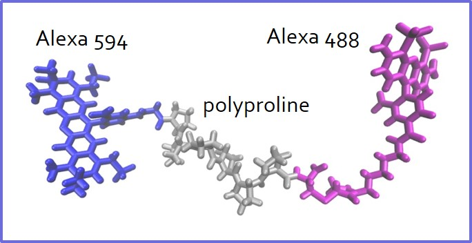
Figure 1: Polyproline 6 labeled with Alexa 488 and Alexa 594 [34].

2 Problem formulation

2.1 Classical form of the problem

In this paper we consider an interface problem describing the electrostatic potential in a system consisting of a (macro)molecule embedded in a solution, e.g., of a solvent like water and a solute like $\rm{NaCl}$. The computational domain $\Omega\subset\mathbb{R}^{d}$ is assumed to be bounded with Lipschitz boundary $\partial\Omega$. The domain containing the molecule is denoted by $\Omega_{m}\subset\mathbb{R}^{d}$ and assumed to be strictly inside $\Omega$, i.e. $\overline{\Omega}_{m}\subset\Omega$ and also with Lipschitz boundary. The domain containing the solution with the moving ions of the solute is denoted by $\Omega_{s}$ and is defined by $\Omega_{s}=\Omega\setminus\overline{\Omega}_{m}$. The interface of $\Omega_{m}$ and $\Omega_{s}$ is denoted by $\Gamma=\overline{\Omega}_{m}\cap\overline{\Omega}_{s}=\partial\Omega_{m}$, and the outward unit normal vector on $\partial\Omega_{m}=\Gamma$ by $n$.

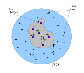
Figure 2: Computational domain $\Omega$ with molecular domain $\Omega_{m}$ and solution domain $\Omega_{s}$.

Assuming that we have only two ion species in the solution with the same concentration $c(x)$ (which are univalent but with opposite charge, i.e $q_{j}=(-1)^{j}e_{c},\,j=1,2,\,e_{c}>0$), the interface problem reads as follows

$$-\nabla\cdot\left(\epsilon\nabla\phi\right)+8\pi ce_{c}\,\sinh\left(\frac{e_{c}\phi}{k_{B}T}\right) = 4\pi\sum\limits_{i=1}^{N}{q_{i}\delta_{x_{i}}(x)}\quad\text{in }\Omega_{m}\cup\Omega_{s},$$ (2.1a)

$$\left[\phi\right]_{\Gamma} = 0,$$ (2.1b)

$$\left[\epsilon\nabla\phi\cdot n\right]_{\Gamma} = 0,$$ (2.1c)

$$\phi = \psi\quad\text{on }\partial\Omega,$$ (2.1d)

where $\psi\in C^{0,1}(\partial\Omega)$ and $e_{c}$ is the electron charge. The function $c(x)\geq 0$ is given by

$$c(x)=\left\{\begin{array}[]{lll}&0,&x\in\Omega_{m},\\ &c^{\infty},&x\in\Omega_{s},\end{array}\right.$$

where $c^{\infty}$ is a positive constant and represents the bulk concentration of the two ion species in solution, $k_{B}$ is the Boltzmann constant, $T$ is the absolute temperature (constant), $x_{i}$ is the position of the $i$-th fixed point charge in the molecular domain $\Omega_{m}$, $\delta_{x_{i}}$ is the delta distribution centered at $x_{i}$, and $\phi(x)$ is the unknown electrostatic potential. The coefficient $\epsilon(x)$ (dielectric constant) is piecewise constant, i.e.

$$\epsilon(x)=\left\{\begin{aligned} &\epsilon_{m},&x&\in\Omega_{m},\\ &\epsilon_{s},&x&\in\Omega_{s}.\end{aligned}\right.$$ (2.2)

Introduce the new variable $\tilde{\phi}=\frac{e_{c}\phi}{k_{B}T}$. Then writing $q_{i}=z_{i}e_{c}$, where $z_{i}\in\mathbb{Z}$ we obtain the dimensionless form of (2.1):

$$-\nabla\cdot\left(\epsilon(x)\nabla\tilde{\phi}\right)+k^{2}(x)\sinh\left(\tilde{\phi}\right) = \frac{4\pi e_{c}^{2}}{k_{B}T}\sum\limits_{i=1}^{N}{z_{i}\delta_{x_{i}}(x)}\quad\text{in }\Omega_{m}\cup\Omega_{s},$$ (2.3a)

$$\left[\tilde{\phi}\right]_{\Gamma} = 0,$$ (2.3b)

$$\left[\epsilon\nabla\tilde{\phi}\cdot n\right]_{\Gamma} = 0,$$ (2.3c)

$$\tilde{\phi} = g\quad\text{on }\partial\Omega,$$ (2.3d)

where $g=\frac{e_{c}\psi}{k_{B}T}$ and the coefficient $k(x)$ is given by

$$k^{2}(x)=\frac{8\pi c(x)e_{c}^{2}}{k_{B}T}=\left\{\begin{aligned} &k_{m}^{2}=0,&x&\in\Omega_{m},\\ &k_{s}^{2}=\frac{8\pi c^{\infty}e_{c}^{2}}{k_{B}T},&x&\in\Omega_{s}.\end{aligned}\right.$$ (2.4)

Equation (2.1a) is often referred to as the Poisson-Boltzmann equation (PBE) [20], [13], [25]. Equations (2.1b) and (2.1c) are the interface conditions. Here $\left[f\right]_{\Gamma}$ denotes the jump of a function $f:\Omega_{m}\cup\Omega_{s}\to\mathbb{R}$ that is uniformly continuous in $U_{\Gamma}\cap\Omega_{m}$ and $U_{\Gamma}\cap\Omega_{s}$, where $U_{\Gamma}$ is a neighborhood of $\Gamma$, that is,

$$\left[f\right]_{\Gamma}:=\gamma_{\Gamma}\left(f{\mathord{\upharpoonright}_{\Omega_{m}}}\right)-\gamma_{\Gamma}\left(f{\mathord{\upharpoonright}_{\Omega_{s}}}\right)$$

with $\gamma_{\Gamma}(f{\mathord{\upharpoonright}_{X}})$ denoting the unique extension of $f{\mathord{\upharpoonright}_{X}}$ by continuity to $\Gamma$ and $f{\mathord{\upharpoonright}_{X}}$ denoting the restriction of $f$ to $X\in\{\Omega_{m},\Omega_{s}\}$.

We notice that in fact the physical problem prescribes a vanishing potential at infinite distance from the boundary of $\Omega_{m}$, i.e., $\lim_{|x|\to\infty}{\phi(x)}=0$. In practice, one uses a bounded computational domain and imposes the boundary condition (2.1d) instead, where the function $\psi$ can usually be calculated accurately enough by solving a simpler problem, possibly with a known analytical solution.

2.2 2-term and 3-term splittings of the solution

A commonly used technique (see, e.g. [23]) to solve and analyze problem (2.3) is to split the solution according to $\tilde{\phi}=G+u$, where $G$ is the analytically known solution of the problem

$$-\nabla\cdot(\epsilon_{m}\nabla G)=\frac{4\pi e_{c}^{2}}{k_{B}T}\sum\limits_{i=1}^{N}{z_{i}\delta_{x_{i}}(x)},\quad\text{on }\mathbb{R}^{d},\,d\in\{2,3\}.$$ (2.5)

If $d=2$, then

$$G=\sum\limits_{i=1}^{N}{G_{i}}=-\frac{2\pi e_{c}^{2}}{\epsilon_{m}k_{B}T}\sum\limits_{i=1}^{N}{z_{i}\ln{|x-x_{i}|}}$$ (2.6)

and if $d=3$

$$G=\sum\limits_{i=1}^{N}{G_{i}}=\frac{e_{c}^{2}}{\epsilon_{m}k_{B}T}\sum\limits_{i=1}^{N}{\frac{z_{i}}{|x-x_{i}|}}.$$ (2.7)

The regular component $u$ is assumed to be a function in $H^{1}(\Omega)$. Since $\epsilon_{m}$ and $\epsilon_{s}$ are constants, the problem for $u$ is as follows:

$$-\nabla\cdot\left(\epsilon\nabla u\right)+k^{2}\sinh\left(u+G\right) = 0\quad\text{in }\Omega_{m}\cup\Omega_{s},$$ (2.8a)

$$\left[u\right]_{\Gamma} = 0,$$ (2.8b)

$$\left[\epsilon\nabla u\cdot n\right]_{\Gamma} = -\left[\epsilon\nabla G\cdot n\right]_{\Gamma},$$ (2.8c)

$$u = g-G\quad\text{on}\quad\partial\Omega.$$ (2.8d)

For further analysis of (2.8), it is convenient to split $u$ into $u^{N}+u^{L}$, where $u^{L}$ solves

$$-\nabla\cdot\left(\epsilon\nabla u^{L}\right) = 0\quad\text{in }\Omega_{m}\cup\Omega_{s},$$ (2.9a)

$$\left[u^{L}\right]_{\Gamma} = 0,$$ (2.9b)

$$\left[\epsilon\frac{\partial u^{L}}{\partial n}\right]_{\Gamma} = -\left[\epsilon\nabla G\cdot n\right],$$ (2.9c)

$$u^{L} = g-G,\quad\text{on }\partial\Omega,$$ (2.9d)

and $u^{N}$ solves the homogeneous nonlinear problem

$$-\nabla\cdot\left(\epsilon\nabla u^{N}\right)+k^{2}\sinh(u^{N}+G+u^{L}) = 0\quad\text{in }\Omega_{m}\cup\Omega_{s},$$ (2.10a)

$$\left[u^{N}\right]_{\Gamma} = 0,$$ (2.10b)

$$\left[\epsilon\frac{\partial u^{N}}{\partial n}\right]_{\Gamma} = 0,$$ (2.10c)

$$u^{N} = 0,\quad\text{on }\partial\Omega.$$ (2.10d)

Notice that the problem (2.10) uses the exact solution $u^{L}$ of (2.9).

However, the splitting $\tilde{\phi}=G+u$ causes numerical instability when $G$ and $u$ are with opposite signs but nearly of the same absolute value in $\Omega_{s}$. This mostly happens when $\epsilon_{m}\ll\epsilon_{s}$ (see, e.g. [25]). In order to overcome this difficulty one may use a splitting of $\tilde{\phi}$ into $3$ components, two of which add up to zero in $\Omega_{s}$. Such a splitting is given by

$$\tilde{\phi}=G+u^{H}+u,$$ (2.11)

such that $\tilde{\phi}=u$ in $\Omega_{s}$, i.e. $u^{H}=-G$ in $\Omega_{s}$, and has been used in [25].

The no-jump condition (2.3b) on $\Gamma$ can be expressed as:

$$\left[\tilde{\phi}\right]_{\Gamma}:=\gamma_{\Gamma}\left((G+u^{H}+u){\mathord{\upharpoonright}_{\Omega_{m}}}\right)-\gamma_{\Gamma}\left(u{\mathord{\upharpoonright}_{\Omega_{s}}}\right)=0.$$

If we further require $u^{H}$ to be continuous across $\Gamma$, then $\left[u\right]_{\Gamma}=0$. Consequently, we arrive at the following system of equations:

$$u^{H} = -G\quad\text{in }\Omega_{s},$$

$$-\nabla\cdot\left(\epsilon_{s}\nabla u\right)+k^{2}\sinh(u) = 0\quad\text{in }\Omega_{s},$$ (2.12)

and

$$-\nabla\cdot\left(\epsilon_{m}\nabla\left(u+u^{H}+G\right)\right)=\frac{4\pi e_{c}^{2}}{k_{B}T}\sum\limits_{i=1}^{N}{z_{i}\delta_{x_{i}}(x)}\quad\text{in }\Omega_{m}.$$ (2.13)

Hence, defining $u^{H}$ in $\Omega_{m}$ to be the solution of

$$-\Delta u^{H} = 0\quad\text{in}\quad\Omega_{m},$$ (2.14a)

$$u^{H} = -G\quad\text{on}\quad\Gamma=\partial\Omega_{m},$$ (2.14b)

taking into account (2.5) and recalling that $\epsilon_{m}$ is a constant, we get

$$-\nabla\cdot\left(\epsilon_{m}\nabla u\right)=0\quad\text{in }\Omega_{m}.$$ (2.15)

In view of (2.2) and (2.4) we can represent (2.2) and (2.15) in one common form, namely,

$$-\nabla\cdot\left(\epsilon\nabla u\right)+k^{2}\sinh(u)=0\quad\text{in }\Omega_{m}\cup\Omega_{s}.$$

In order to find the interface condition for the flux $\epsilon\nabla u\cdot n$, we note that $\left[\epsilon\frac{\partial\tilde{\phi}}{\partial n}\right]=0.$ From this condition, we deduce the relation

$$\gamma_{\Gamma}\left({\epsilon_{m}\frac{\partial u}{\partial n}}{\mathord{\upharpoonright}_{\Omega_{m}}}\right)+\gamma_{\Gamma}\left(\epsilon_{m}\frac{\partial\left(u^{H}+G\right)}{\partial n}{\mathord{\upharpoonright}_{\Omega_{m}}}\right)=\gamma_{\Gamma}\left(\epsilon_{s}\frac{\partial u}{\partial n}{\mathord{\upharpoonright}_{\Omega_{s}}}\right)$$

or, equivalently,

$$\left[\epsilon\frac{\partial u}{\partial n}\right]_{\Gamma}=-\gamma_{\Gamma}\left(\epsilon_{m}\frac{\partial\left(u^{H}+G\right)}{\partial n}{\mathord{\upharpoonright}_{\Omega_{m}}}\right)=:g_{\Gamma}$$

Thus, we arrive at the following interface problem for the regular component $u$:

$$-\nabla\cdot\left(\epsilon\nabla u\right)+k^{2}\sinh(u) = 0\quad\text{in }\Omega_{m}\cup\Omega_{s},$$ (2.16a)

$$\left[u\right]_{\Gamma} = 0,$$ (2.16b)

$$\left[\epsilon\frac{\partial u}{\partial n}\right]_{\Gamma} = g_{\Gamma},$$ (2.16c)

$$u = g,\quad\text{on }\partial\Omega.$$ (2.16d)

For further analysis of problem (2.16), we split the regular component $u$ into $u^{N}+u^{L}$, where $u^{L}$ solves the linear nonhomogeneous interface problem

$$-\nabla\cdot\left(\epsilon\nabla u^{L}\right) = 0\quad\text{in }\Omega_{m}\cup\Omega_{s},$$ (2.17a)

$$\left[u^{L}\right]_{\Gamma} = 0,$$ (2.17b)

$$\left[\epsilon\frac{\partial u^{L}}{\partial n}\right]_{\Gamma} = g_{\Gamma},$$ (2.17c)

$$u^{L} = g,\quad\text{on }\partial\Omega$$ (2.17d)

and $u^{N}$ solves the homogeneous nonlinear problem

$$-\nabla\cdot\left(\epsilon\nabla u^{N}\right)+k^{2}\sinh(u^{N}+u^{L}) = 0\quad\text{in }\Omega_{m}\cup\Omega_{s},$$ (2.18a)

$$\left[u^{N}\right]_{\Gamma} = 0,$$ (2.18b)

$$\left[\epsilon\frac{\partial u^{N}}{\partial n}\right]_{\Gamma} = 0,$$ (2.18c)

$$u^{N} = 0,\quad\text{on }\partial\Omega.$$ (2.18d)

Again, (2.18) includes the exact solution of (2.17) as a known function.

2.3 Variational form of the problem

It is easy to see that the generalized solution

$$u^{L}\in H_{g}^{1}(\Omega)=\{v\in H^{1}(\Omega):\gamma_{\partial\Omega}(v)=g\text{ on }\partial\Omega\}$$

of (2.17) solves the variational problem

$$a(u^{L},v)=\langle g_{\Gamma},\gamma_{\Gamma}(v)\rangle_{\Gamma},\forall v\in H_{0}^{1}(\Omega),$$ (2.19)

where

$$a(u,v):=\int_{\Omega}{\epsilon\nabla u\cdot\nabla vdx},$$ (2.20)

$\gamma_{\partial\Omega}(v)$ is the trace of $v$ on $\partial\Omega$, $\gamma_{\Gamma}(v)$ is the trace of $v$ on $\Gamma$, and $\langle.,.\rangle_{\Gamma}$ denotes the duality pairing in $H^{-1/2}(\Gamma)\times H^{1/2}(\Gamma)$.

If the distribution $g_{\Gamma}\in H^{-1/2}(\Gamma)$ is regular so that the action on any function $v\in H^{1/2}$ can be represented by the integral $\int_{\Gamma}g_{\Gamma}vds$, where $g_{\Gamma}\in L^{2}$, then we the right hand side in (2.19) can be written in the form $\int_{\Gamma}g_{\Gamma}\gamma_{\Gamma}ds$ for all $v\in H_{0}^{1}(\Omega)$.
For the $3$-term regularization, if $\nabla u^{H}$ is uniformly continuous in a neighborhood of the interface $\Gamma$, since $\nabla G$ is smooth in a neighborhood of the interface $\Gamma$, then we have

$$g_{\Gamma}=-\gamma_{\Gamma}\left(\epsilon_{m}\frac{\partial(u^{H}+G)}{\partial n}{\mathord{\upharpoonright}_{\Omega_{m}}}\right)\in L^{2}(\Gamma)$$

and in this case we can use $\int\limits_{\Gamma}{g_{\Gamma}vds}$ on the RHS of (2.19). We can also write

$$g_{\Gamma}=-\gamma_{\Gamma}(\epsilon_{m}\nabla u^{H}\cdot n{\mathord{\upharpoonright}_{\Omega_{m}}})-\gamma_{\Gamma}(\epsilon_{m}\nabla G\cdot n{\mathord{\upharpoonright}_{\Omega_{s}}}).$$ (2.21)

Therefore, we see that if $\nabla u^{H}$ is only in $H(\operatorname{div};\Omega_{m})$, then the functional $g_{\Gamma}\in H^{-1/2}(\Gamma)$ is defined as follows

$$\langle g_{\Gamma},v\rangle_{\Gamma}=-\langle\gamma_{n,\Omega_{m}}(\epsilon_{m}\nabla u^{H}),v\rangle_{\Gamma}+\langle\gamma_{n,\Omega_{s}}(\epsilon_{m}\nabla G),v\rangle_{\Gamma},\,\forall v\in H^{1/2}(\Gamma),$$ (2.22)

where $\gamma_{n,X}$ denotes the normal trace in the space $H(\operatorname{div};X)$. Now, using the divergence formula, the weak formulation (2.19) can be rewritten as:

$$\begin{aligned} &\text{Find }u^{L}\in H_{g}^{1}(\Omega)\text{ such that}&\\ &\int\limits_{\Omega}{\epsilon\nabla u^{L}\cdot\nabla vdx}=-\int\limits_{\Omega_{m}}{\operatorname{div}{(\epsilon_{m}\nabla u^{H})}vdx}-\int\limits_{\Omega_{m}}{\epsilon_{m}\nabla u^{H}\cdot\nabla vdx}\\ &+\int\limits_{\Omega_{s}}{\operatorname{div}{(\epsilon_{m}\nabla G)}vdx}+\int\limits_{\Omega_{s}}{\epsilon_{m}\nabla G\cdot\nabla vdx}\\ &=-\int\limits_{\Omega_{m}}{\epsilon_{m}\nabla u^{H}\cdot\nabla vdx}+\int\limits_{\Omega_{s}}{\epsilon_{m}\nabla G\cdot\nabla vdx},\,\forall v\in H_{0}^{1}(\Omega).\end{aligned}$$ (2.23)

For the $2$-term regularization, $g_{\Gamma}$ is known exactly, and it is given by the relation

$$g_{\Gamma}=-[\epsilon\nabla G\cdot n]\in L^{2}(\Gamma)$$

Here is used the fact that $\nabla G$ is smooth in a neighborhood of the interface $\Gamma$. Since

$$\langle g_{\Gamma},\gamma_{\Gamma}(v)\rangle_{\Gamma}=\int\limits_{\Omega}{(\epsilon_{m}-\epsilon)\nabla G\cdot\nabla vdx}=\int\limits_{\Omega_{s}}{(\epsilon_{m}-\epsilon_{s})\nabla G\cdot\nabla vdx},\,\forall v\in H_{0}^{1}(\Omega),$$ (2.24)

the integral relation that defines $u^{L}$ in the $2$-term regularization comes in the form:

$$\begin{aligned} &\text{Find }u^{L}\in H_{g-G}^{1}(\Omega)\text{ such that}\\ &\int\limits_{\Omega}{\epsilon\nabla u^{L}\cdot\nabla vdx}=\int\limits_{\Omega_{s}}{(\epsilon_{m}-\epsilon_{s})\nabla G\cdot\nabla vdx},\,\forall v\in H_{0}^{1}(\Omega),\,\forall v\in H_{0}^{1}(\Omega).\end{aligned}$$ (2.25)

The well-posedness of (2.19) (or, equivalently, (2.23)) follows from the Lax-Milgram Lemma. Moreover, if $\partial\Omega$ and $\Gamma$ are sufficiently smooth, for example, if $\partial\Omega$ is Lipschitz and $\Gamma$ is $C^{1}$, then from [16] it follows that $u^{L}\in W^{1,p}(\Omega)$ for some $p>d=3$. Using the embedding theorems, we conclude that $u^{L}\in L^{\infty}(\Omega)$: Denote by $V^{*}$ the topological dual of a Banach space $V$ and by $p^{\prime}=\frac{p}{p-1}$ the Hölder conjugate of $p$. It has been shown in [16] that for $\partial\Omega$ being Lipschitz and $\Gamma\in C^{1}$, $\Gamma$ is not touching $\partial\Omega$, there exists $p>3$ such that $-\nabla\cdot(\epsilon(x)\nabla u):W_{0}^{1,q}(\Omega)\to W^{-1,q}(\Omega)=\left(W_{0}^{1,q^{\prime}}\right)^{*}$ is a topological isomorphism for all $q\in(p^{\prime},p)$. In addition, if $\partial\Omega$ is also $C^{1}$, then $p$ may be taken to be $\infty$. This result is useful, because for $q>d=3$ we know that the functions in $W^{1,q}(\Omega)$ are Hölder continuous and thus in $L^{\infty}(\Omega)$.

We can then apply this result to the homogenized version of problem (2.19): find $u_{0}^{L}\in H_{0}^{1}(\Omega)$ such that

$$a(u_{0}^{L},v)=-a(u_{g}^{L},v)+\langle g_{\Gamma},\gamma_{\Gamma}(v)\rangle_{\Gamma},\,\forall v\in H_{0}^{1}(\Omega),$$

where $u^{L}=u_{g}^{L}+u_{0}^{L}\in H_{g}^{1}(\Omega)$ with $u_{g}^{L}\in W^{1,q}(\Omega)\cap L^{\infty}(\Omega)$, $q$ is a fixed number such that $3<q<p$, and $\gamma_{\partial\Omega}(u_{g}^{L})=g$. Note that in order to apply Theorem 1.1 in [16] the functionals $\langle g_{\Gamma},\gamma_{\Gamma}(.)\rangle_{\Gamma}$ and $-a(u_{g}^{L},.)$ need to be well defined, bounded and linear over $W_{0}^{1,q^{\prime}}$, where $q^{\prime}=\frac{q}{q-1}<\frac{3}{2}$.

To show the boundedness of these functionals we assume additionally that $\Gamma\in C^{1,1}$. In this case, by applying Theorem 2.4.2.5 from [28] we get that $u^{H}\in W^{2,2}(\Omega_{m})$ and thus by the Sobolev embedding theorem for $d=3$, $\nabla u^{H}\in L^{6}(\Omega_{m})$ and for $d=2$, $\nabla u^{H}\in L^{r}(\Omega_{m}),\,\forall r:1\leq r<\infty$. Then, for the $3$-term splitting, using (2.23) and applying Hölder inequality, we obtain

$$\left|\langle g_{\Gamma},\gamma_{\Gamma}(v)\rangle_{\Gamma}\right|\leq\epsilon_{m}\left(\|\nabla u^{H}\|_{L^{q}(\Omega_{m})}+\|\nabla G\|_{L^{q}(\Omega_{s})}\right)\|v\|_{W^{1,q^{\prime}}(\Omega)},\,\forall v\in W_{0}^{1,q^{\prime}},$$

$$\left|-a(u_{g}^{L},v)\right|\leq\epsilon_{\max}\|u_{g}^{L}\|_{W^{1,q}(\Omega)}\|v\|_{W^{1,q^{\prime}}(\Omega)},\,\forall v\in W_{0}^{1,q^{\prime}}(\Omega).$$

For the $2$-term splitting we will have $u^{L}=u_{g-G}^{L}+u_{0}^{L}$ where $u_{g-G}^{L}\in W^{1,q}(\Omega)\cap L^{\infty}(\Omega)$ with $\gamma_{\partial\Omega}(u_{g-G}^{L})=g-G$ and $u_{0}^{L}\in H_{0}^{1}(\Omega)$. Thus, using (2.25) we obtain, as before,

$$\left|\langle g_{\Gamma},\gamma_{\Gamma}(v)\rangle_{\Gamma}\right|\leq(\epsilon_{m}-\epsilon_{s})\|\nabla G\|_{L^{q}(\Omega_{s})}\|v\|_{W^{1,q^{\prime}}(\Omega)},\,\forall v\in W_{0}^{1,q^{\prime}},$$

$$\left|-a(u_{g-G}^{L},v)\right|\leq\epsilon_{\max}\|u_{g-G}^{L}\|_{W^{1,q}(\Omega)}\|v\|_{W^{1,q^{\prime}}(\Omega)},\,\forall v\in W_{0}^{1,q^{\prime}}(\Omega).$$

Another way to see that $u^{L}\in L^{\infty}(\Omega)$ without assuming that $\Gamma$ is $C^{1}$ and only assuming that it is Lipschitz is to apply Theorem B.2 from Kinderlehrer and Stampacchia [8]. For this, we need only to ensure that for some $s>d$ it holds $\nabla G\in\left[L^{s}(\Omega_{s})\right]^{d}$, $\nabla u^{H}\in\left[L^{s}(\Omega_{m})\right]^{d}$ in the case of the 3-term splitting and that $\nabla G\in\left[L^{s}(\Omega_{s})\right]^{d}$ in the case of the 2-term splitting (just apply the result of Theorem B.2 to the homogenized versions of (2.23) and (2.25)). Indeed, $\nabla G\in\left[L^{s}(\Omega_{s})\right]^{d}$ since $G$ is smooth in $\Omega_{s}$ and $u^{H}\in W^{1,p}(\Omega)$ for some $p>d$ according to [16].

Definition 2.1.

If $u^{N}\in H_{0}^{1}(\Omega)$ is such that $b(x,u^{N}+u^{L})v\in L^{1}(\Omega)\,\forall v\in H_{0}^{1}(\Omega)\cap L^{\infty}(\Omega)$ and

$$a(u^{N},v)+\int_{\Omega}{b(x,u^{N}+u^{L})vdx}=0,\,\forall v\in H_{0}^{1}(\Omega)\cap L^{\infty}(\Omega),$$ (2.26)

where $a(.,.)$ is defined in (2.20) and $b(x,s):=k^{2}(x)\sinh(s)$ then $u^{N}$ is called a weak solution of (2.18). Similarly, we call $u^{N}$ a weak solution of (2.10) if $u^{N}\in H_{0}^{1}(\Omega)$ and $u^{N}$ is such that $b(x,u^{N}+G+u^{L})v\in L^{1}(\Omega)\,\forall v\in H_{0}^{1}(\Omega)\cap L^{\infty}(\Omega)$ and

$$a(u^{N},v)+\int_{\Omega}{b(x,u^{N}+G+u^{L})vdx}=0,\,\forall v\in H_{0}^{1}(\Omega)\cap L^{\infty}(\Omega).$$ (2.27)

According to [21], we have the following proposition.

Proposition 2.1.

Problem (2.26) has a unique weak solution $u^{N}\in H_{0}^{1}(\Omega)$, which belongs to $L^{\infty}(\Omega)$ and satisfies $\|u^{N}\|_{L^{\infty}(\Omega)}\leq\|u^{L}\|_{L^{\infty}(\Omega_{s})}$. Similarly, problem (2.27) has an unique weak solution $u^{N}$ which belongs to $L^{\infty}(\Omega)$ and satisfies $\|u^{N}\|_{L^{\infty}(\Omega)}\leq\|G+u^{L}\|_{L^{\infty}(\Omega_{s})}$. As a consequence, the test functions in (2.26) and (2.27) can be taken in $H_{0}^{1}(\Omega)$.

In certain situations, when using the 3-term splitting, it is better not to split the regular component $u$ additionally into $u^{L}+u^{N}$. Such a situation may arise if the norm of $u^{L}+u^{N}$ is much smaller than the norm of at least one of $u^{L}$ and $u^{N}$ since then small relative errors in $u^{L}$ and $u^{N}$ become substantial relative errors in the sum $u^{L}+u^{N}$. Therefore, we also consider solving equation (2.16).

Definition 2.2.

$u$ is called a weak solution of (2.16) if $u\in H_{g}^{1}(\Omega)$ and $u$ is such that $b(x,u)v\in L^{1}(\Omega)\,\forall v\in H_{0}^{1}(\Omega)\cap L^{\infty}(\Omega)$ and

$$\begin{aligned} &a(u,v)+\int_{\Omega}{b(x,u)vdx}=\langle g_{\Gamma},\gamma_{\Gamma}(v)\rangle_{\Gamma}\\ &=-\int\limits_{\Omega_{m}}{\epsilon_{m}\nabla u^{H}\cdot\nabla vdx}+\int\limits_{\Omega_{s}}{\epsilon_{m}\nabla G\cdot\nabla vdx},\text{ for all }v\in H_{0}^{1}(\Omega)\cap L^{\infty}(\Omega).\end{aligned}$$ (2.28)

To see that (2.28) has a solution, we can define the energy functional $J$ over $H_{g}^{1}(\Omega)$, like in [21]

$$J(v):=\left\{\begin{aligned} &\int\limits_{\Omega}{\left[\frac{\epsilon(x)}{2}\left|\nabla v\right|^{2}+k^{2}\cosh(v)+\epsilon_{m}\nabla u^{H}\cdot\nabla v\mathbbm{1}_{\Omega_{m}}-\epsilon_{m}\nabla G\cdot\nabla v\mathbbm{1}_{\Omega_{s}}\right]dx},\\ &\text{ if }k^{2}\cosh(v)\in L^{1}(\Omega),\\ \\ &+\infty,\text{ if }k^{2}\cosh(v)\notin L^{1}(\Omega),\end{aligned}\right.$$ (2.29)

and show the existence of a unique minimizer $u\in H_{g}^{1}(\Omega)$, where $\mathbbm{1}_{X}$ is the indicator function of the set $X$. Then, for the minimizer $u$, using Lebesgue Dominated Convergence Theorem, we can prove that it is indeed a solution to (2.28). The uniqueness of the solution $u$ of (2.28) is proven in a similar way to the approach in [21]. However, an easier approach is to take advantage of the fact that we have already shown existence and uniqueness of a solution to problems (2.23) and (2.26). Moreover, since $u=u^{L}+u^{N}$, where $u^{L}\in L^{\infty}(\Omega)$ is a solution to (2.23) and $u^{N}\in L^{\infty}(\Omega)$ is a solution to (2.26), it follows that $u\in H_{g}^{1}(\Omega)\cap L^{\infty}(\Omega)$.

Hence we have the following proposition.

Proposition 2.2.

Problem (2.28) has a unique weak solution $u\in H_{0}^{1}(\Omega)$ which belongs to $L^{\infty}(\Omega)$. As a consequence, the test functions in (2.28) can be taken to be only in $H_{0}^{1}(\Omega)$.

3 A posteriori error estimates

3.1 Harmonic component $u^{H}$

To get fully reliable error bounds for approximate solutions of problem (2.3), we need first to derive a posteriori estimates for the quantities

$$\|\nabla(u^{H}-\tilde{u}^{H})\|_{L^{2}(\Omega_{m})}\quad\mbox{and}\quad\|\nabla u^{H}-T(\nabla\tilde{u}^{H})\|_{L^{2}(\Omega_{m})},$$

where $\tilde{u}^{H}$ is a conforming approximation of $u^{H}$ and $T(\nabla\tilde{u}^{H})\in H(\operatorname{div};\Omega_{m})$ with $T$ being a regularization operator that maps the numerical flux $\nabla\tilde{u}^{H}$ into $H(\operatorname{div};\Omega_{m})$.

For the first quantity, we have (see [32])

$$\|\nabla(u^{H}-\tilde{u}^{H})\|_{L^{2}(\Omega_{m})}\leq C_{F\Omega_{m}}\|\operatorname{div}\left(T(\nabla\tilde{u}^{H})\right)\|_{L^{2}(\Omega_{m})}+\|\nabla\tilde{u}^{H}-T(\nabla\tilde{u}^{H})\|_{L^{2}(\Omega_{m})}.$$ (3.1)

For the second quantity, we proceed as follows:

$$\|\nabla\tilde{u}^{H}-T(\nabla\tilde{u}^{H})\|_{L^{2}(\Omega_{m})}^{2} = \|\nabla(u^{H}-\tilde{u}^{H})\|_{L^{2}(\Omega_{m})}^{2}$$

$$+ \|\nabla u^{H}-T(\nabla\tilde{u}^{H})\|_{L^{2}(\Omega_{m})}^{2}$$

$$- 2\int\limits_{\Omega_{m}}{\left(T(\nabla\tilde{u}^{H})-\nabla u^{H}\right)\cdot\nabla(\tilde{u}^{H}-u^{H})dx}.$$

Thus, using the Cauchy-Schwartz inequality, we obtain

$$\|\nabla(u^{H}-\tilde{u}^{H})\|_{L^{2}(\Omega_{m})}^{2}+\|\nabla u^{H}-T(\nabla\tilde{u}^{H})\|_{L^{2}(\Omega_{m})}^{2}$$

$$\leq\|\nabla\tilde{u}^{H}-T(\nabla\tilde{u}^{H})\|_{L^{2}(\Omega_{m})}^{2}+2\|\operatorname{div}\left(T(\nabla\tilde{u}^{H})\right)\|_{L^{2}(\Omega_{m})}C_{F\Omega_{m}}\|\nabla(\tilde{u}^{H}-u^{H})\|_{L^{2}(\Omega_{m})}$$

$$\leq\|\nabla\tilde{u}^{H}-T(\nabla\tilde{u}^{H})\|_{L^{2}(\Omega_{m})}^{2}+\|\nabla(u^{H}-\tilde{u}^{H})\|_{L^{2}(\Omega_{m})}^{2}+C_{F\Omega_{m}}^{2}\|\operatorname{div}\left(T(\nabla\tilde{u}^{H})\right)\|_{L^{2}(\Omega_{m})}^{2}$$

Finally,

$$\mathrel{\phantom{=}}\|\nabla u^{H}-T(\nabla\tilde{u}^{H})\|_{L^{2}(\Omega_{m})}$$

$$\leq\left(\|\nabla\tilde{u}^{H}-T(\nabla\tilde{u}^{H})\|_{L^{2}(\Omega_{m})}^{2}+C_{F\Omega_{m}}^{2}\|\operatorname{div}\left(T(\nabla\tilde{u}^{H})\right)\|_{L^{2}(\Omega_{m})}^{2}\right)^{1/2}$$ (3.3)

$$=:M_{\oplus,H}\left(\tilde{u}^{H},T(\nabla\tilde{u}^{H})\right)$$

If $T(\nabla\tilde{u}^{H})$ is additionally equilibrated (for example using the patchwise equilibration technique in [6]) then both estimates (3.1) and (3.1) follow from (3.1) (Prager-Synge estimate).

3.2 Linear nonhomogeneous problem

In this section, we show how to obtain a guaranteed bound on the energy norm of the error $\nabla(\tilde{u}^{L}-v)$. Here $v$ is some conforming approximation of $\tilde{u}^{L}$, the weak solution of the interface problem (2.23) with $\nabla u^{H}$ replaced by $T(\nabla\tilde{u}^{H})$. The function $\tilde{u}^{H}$ is some conforming approximation of $u^{H}$ and $T$ is some operator that maps the numerical flux $\epsilon\nabla\tilde{u}^{H}$ into $H(\operatorname{div};\Omega_{m})$. If $\nabla\tilde{u}^{H}$ is already in $H(\operatorname{div};\Omega_{m})$, then we can take $T$ to be the identity. The error estimate that we derive here is similar to the one derived in Chapter 4 from [32] with the exception that here we avoid involving the trace constant in $\Omega_{m}$ by exactly prescribing the jump condition on the interface $\Gamma$.

The function $\tilde{u}^{L}$ satisfies the weak formulation:

$$\text{Find }\tilde{u}^{L}\in H_{g}^{1}(\Omega)\text{ such that}$$

$$\mathrel{\phantom{=}}\underline{\int\limits_{\Omega}{\epsilon\nabla\tilde{u}^{L}\cdot\nabla\phi dx}=-\int\limits_{\Omega_{m}}{\epsilon_{m}T(\nabla\tilde{u}^{H})\cdot\nabla\phi dx}+\int\limits_{\Omega_{s}}{\epsilon_{m}\nabla G\cdot\nabla\phi dx}}$$

$$=-\int\limits_{\Omega_{m}}{\operatorname{div}(\epsilon_{m}T(\nabla\tilde{u}^{H}))\phi dx}-\int\limits_{\Omega_{m}}{\epsilon_{m}T(\nabla\tilde{u}^{H})\cdot\nabla\phi dx}$$

$$+\int\limits_{\Omega_{s}}{\operatorname{div}(\epsilon_{m}\nabla G)\phi dx}+\int\limits_{\Omega_{s}}{\epsilon_{m}\nabla G\cdot\nabla\phi dx}+\int\limits_{\Omega_{m}}{\operatorname{div}(\epsilon_{m}T(\nabla\tilde{u}^{H}))\phi dx}$$

$$=-\langle\gamma_{n,\Omega_{m}}(\epsilon_{m}T(\nabla\tilde{u}^{H})),\gamma_{\Gamma}(\phi)\rangle_{\Gamma}+\langle\gamma_{n,\Omega_{s}}(\epsilon_{m}\nabla G),\gamma_{\Gamma}(\phi)\rangle_{\Gamma}$$

$$+\int\limits_{\Omega_{m}}{\operatorname{div}(\epsilon_{m}T(\nabla\tilde{u}^{H}))\phi dx},\,\forall\phi\in H_{0}^{1}(\Omega).$$ (3.4)

Now, let $\tilde{y}_{L}^{*}=y^{*}_{\tilde{g}_{\Gamma}}+\tilde{y}_{0}^{*}$, where

$$\begin{aligned} &y^{*}_{\tilde{g}_{\Gamma}}=-\epsilon_{m}T(\nabla\tilde{u}^{H})\mathbbm{1}_{\Omega_{m}}+\epsilon_{m}\nabla G\mathbbm{1}_{\Omega_{s}},\\ &\tilde{y}_{0}^{*}\in H(\operatorname{div};\Omega),\end{aligned}$$ (3.5)

and $\mathbbm{1}_{X}$ is the indicator function of the set $X$. From (3.5) it follows that ${\tilde{y}_{L}^{*}}_{\mathord{\upharpoonright}_{\Omega_{m}}}\in H(\operatorname{div};\Omega_{m})$ and ${\tilde{y}_{L}^{*}}_{\mathord{\upharpoonright}_{\Omega_{s}}}\in H(\operatorname{div};\Omega_{s})$. From (3.2), testing with functions $\phi\in H_{0}^{1}(\Omega_{m})$ and $\phi\in H_{0}^{1}(\Omega_{s})$, we see that

$$\begin{aligned} (\epsilon\nabla\tilde{u}^{L})_{\mathord{\upharpoonright}_{\Omega_{m}}}&\in H(\operatorname{div};\Omega_{m}),\,\operatorname{div}\left((\epsilon\nabla\tilde{u}^{L})_{\mathord{\upharpoonright}_{\Omega_{m}}}\right)=-\operatorname{div}\left(\epsilon_{m}T(\nabla\tilde{u}^{H})\right),\\ (\epsilon\nabla\tilde{u}^{L})_{\mathord{\upharpoonright}_{\Omega_{s}}}&\in H(\operatorname{div};\Omega_{s}),\,\operatorname{div}\left((\epsilon\nabla\tilde{u}^{L})_{\mathord{\upharpoonright}_{\Omega_{m}}}\right)=0.\end{aligned}$$ (3.6)

Let $v\in H_{g}^{1}(\Omega)$ be a conforming approximation of $\tilde{u}^{L}$. We proceed with the derivation of an a posteriori estimate for ${\left|\kern-1.07639pt\left|\kern-1.07639pt\left|\nabla(\tilde{u}^{L}-v)\right|\kern-1.07639pt\right|\kern-1.07639pt\right|}$, where

$${\left|\kern-1.07639pt\left|\kern-1.07639pt\left|q\right|\kern-1.07639pt\right|\kern-1.07639pt\right|}^{2}=\int\limits_{\Omega}{\epsilon|q|^{2}dx},\quad{\left|\kern-1.07639pt\left|\kern-1.07639pt\left|q\right|\kern-1.07639pt\right|\kern-1.07639pt\right|}_{*}^{2}=\int\limits_{\Omega}{\frac{1}{\epsilon}|q|^{2}dx},\quad\forall q\in[L^{2}(\Omega)]^{3}.$$

Furthermore,

$$(\epsilon\nabla(\tilde{u}^{L}-v),\nabla\phi)=-\langle\gamma_{n,\Omega_{m}}\left(\epsilon_{m}T(\nabla\tilde{u}^{H})\right),\gamma_{\Gamma}(\phi)\rangle_{\Gamma}+\langle\gamma_{n,\Omega_{s}}\left(\epsilon_{m}\nabla G\right),\gamma_{\Gamma}(\phi)\rangle_{\Gamma}$$

$$+\int\limits_{\Omega_{m}}{\operatorname{div}\left(\epsilon_{m}T(\nabla\tilde{u}^{H})\right)\phi dx}+\int\limits_{\Omega_{m}}{\operatorname{div}(y^{*}_{\tilde{g}_{\Gamma}}+\tilde{y}_{0}^{*})\phi dx}+\int\limits_{\Omega_{s}}{\operatorname{div}(y^{*}_{\tilde{g}_{\Gamma}}+\tilde{y}_{0}^{*})\phi dx}$$

$$-\langle\gamma_{n,\Omega_{m}}\left(y^{*}_{\tilde{g}_{\Gamma}}+\tilde{y}_{0}^{*}\right),\gamma_{\Gamma}(\phi)\rangle_{\Gamma}-\langle\gamma_{n,\Omega_{s}}\left(y^{*}_{\tilde{g}_{\Gamma}}+\tilde{y}_{0}^{*}\right),\gamma_{\Gamma}(\phi)\rangle_{\Gamma}-(\epsilon\nabla v-\tilde{y}_{L}^{*},\nabla\phi)$$

$$=\int\limits_{\Omega_{m}}{\operatorname{div}\left(\epsilon_{m}T(\nabla\tilde{u}^{H})\right)\phi dx}+\int\limits_{\Omega_{m}}{\operatorname{div}(y^{*}_{\tilde{g}_{\Gamma}}+\tilde{y}_{0}^{*})\phi dx}+\int\limits_{\Omega_{s}}{\operatorname{div}(y^{*}_{\tilde{g}_{\Gamma}}+\tilde{y}_{0}^{*})\phi dx}$$

$$-(\epsilon\nabla v-\tilde{y}_{L}^{*},\nabla\phi)=\int\limits_{\Omega_{m}}{\operatorname{div}\tilde{y}_{0}^{*}\phi dx}+\int\limits_{\Omega_{s}}{\operatorname{div}\tilde{y}_{0}^{*}\phi dx}-(\epsilon\nabla v-\tilde{y}_{L}^{*},\nabla\phi)$$

$$=(\operatorname{div}\tilde{y}_{0}^{*},\phi)-(\epsilon\nabla v-\tilde{y}_{L}^{*},\nabla\phi),$$

where we have used (3.5). Now, taking $\phi=\tilde{u}^{L}-v\in H_{0}^{1}(\Omega)$ we have that

$${\left|\kern-1.07639pt\left|\kern-1.07639pt\left|\nabla(\tilde{u}^{L}-v)\right|\kern-1.07639pt\right|\kern-1.07639pt\right|}^{2}\leq\frac{C_{F\Omega}}{\sqrt{\epsilon_{\min}}}\|\operatorname{div}\tilde{y}_{0}^{*}\|_{L^{2}(\Omega)}{\left|\kern-1.07639pt\left|\kern-1.07639pt\left|\nabla(\tilde{u}^{L}-v)\right|\kern-1.07639pt\right|\kern-1.07639pt\right|}+{\left|\kern-1.07639pt\left|\kern-1.07639pt\left|\epsilon\nabla v-\tilde{y}_{L}^{*}\right|\kern-1.07639pt\right|\kern-1.07639pt\right|}_{*}{\left|\kern-1.07639pt\left|\kern-1.07639pt\left|\nabla(\tilde{u}^{L}-v)\right|\kern-1.07639pt\right|\kern-1.07639pt\right|}$$

and thus by dividing by ${\left|\kern-1.07639pt\left|\kern-1.07639pt\left|\nabla(\tilde{u}^{L}-v)\right|\kern-1.07639pt\right|\kern-1.07639pt\right|}$ we obtain

$${\left|\kern-1.07639pt\left|\kern-1.07639pt\left|\nabla(\tilde{u}^{L}-v)\right|\kern-1.07639pt\right|\kern-1.07639pt\right|}\leq\frac{C_{F\Omega}}{\sqrt{\epsilon_{\min}}}\|\operatorname{div}\tilde{y}_{0}^{*}\|_{L^{2}(\Omega)}+{\left|\kern-1.07639pt\left|\kern-1.07639pt\left|\epsilon\nabla v-\tilde{y}^{*}_{\tilde{g}_{\Gamma}}-\tilde{y}_{0}^{*}\right|\kern-1.07639pt\right|\kern-1.07639pt\right|}_{*}=:M_{\oplus,L}(v,\tilde{y}_{0}^{*})$$ (3.7)

Now, we show that the estimate (3.7) is sharp. For this, take $\tilde{y}_{0}^{*}=\tilde{p}_{L}^{*}-y^{*}_{\tilde{g}_{\Gamma}}$, where $\tilde{p}_{L}^{*}=\epsilon\nabla\tilde{u}^{L}$. We claim that $\tilde{y}_{0}^{*}\in H(\operatorname{div};\Omega)$. Indeed, let $\phi\in H_{0}^{1}(\Omega)$. Then using (3.5), (3.6), and the fact that $G$ is harmonic in $\Omega_{s}$, we obtain

$$\int\limits_{\Omega}{\tilde{y}_{0}^{*}\cdot\nabla\phi dx}=\int\limits_{\Omega}{\tilde{p}_{L}^{*}\cdot\nabla\phi dx}-\int\limits_{\Omega}{y^{*}_{\tilde{g}_{\Gamma}}\cdot\nabla\phi dx}$$

$$=-\langle\gamma_{n,\Omega_{m}}\left(\epsilon_{m}T(\nabla\tilde{u}^{H})\right),\gamma_{\Gamma}(\phi)\rangle_{\Gamma}+\langle\gamma_{n,\Omega_{s}}\left(\epsilon_{m}\nabla G\right),\gamma_{\Gamma}(\phi)\rangle_{\Gamma}$$

$$+\int\limits_{\Omega_{m}}{\operatorname{div}\left(\epsilon_{m}T(\nabla\tilde{u}^{H})\right)\phi dx}-\int\limits_{\Omega_{m}}{\operatorname{div}\left(\epsilon_{m}T(\nabla\tilde{u}^{H})\right)\phi dx}+\langle\gamma_{n,\Omega_{m}}\left(\epsilon_{m}T(\nabla\tilde{u}^{H})\right),\gamma_{\Gamma}(\phi)\rangle_{\Gamma}$$

$$+\int\limits_{\Omega_{s}}{\operatorname{div}(\epsilon_{m}\nabla G)\phi dx}-\langle\gamma_{n,\Omega_{s}}\left(\epsilon_{m}\nabla G\right),\gamma_{\Gamma}(\phi)\rangle_{\Gamma}=0.$$

Thus $\tilde{y}_{0}^{*}\in H(\operatorname{div};\Omega)$ and $\operatorname{div}\tilde{y}_{0}^{*}=0$. Now, substituting $\tilde{y}_{0}^{*}$ into the estimate (3.7) and using again (3.5) and (3.6), we obtain that the RHS of (3.7) is equal to ${\left|\kern-1.07639pt\left|\kern-1.07639pt\left|\nabla(\tilde{u}^{L}-v)\right|\kern-1.07639pt\right|\kern-1.07639pt\right|}$. In practice, to find a sharp bound on the error we can do a minimization of the majorant $M_{\oplus,L}(v,\tilde{y}_{0}^{*})$ in $\tilde{y}_{0}^{*}$ over a finite dimensional subspace of $H(\operatorname{div};\Omega)$. However, it is more convenient to minimize the squared majorant $M_{\oplus,L}^{2}(v,\tilde{y}_{0}^{*};\alpha)$ simultaneously over $\alpha\in\mathbb{R}_{>0}:=\{x\in\mathbb{R}:x>0\}$ and $\tilde{y}_{0}^{*}$ in a finite dimensional subspace of $H(\operatorname{div};\Omega)$, cf. [32]:

$${\left|\kern-1.07639pt\left|\kern-1.07639pt\left|\nabla(\tilde{u}^{L}-v)\right|\kern-1.07639pt\right|\kern-1.07639pt\right|}^{2}\leq M_{\oplus,L}^{2}(v,\tilde{y}_{0}^{*})$$

$$\leq(1+\alpha)\frac{C_{F\Omega}}{\epsilon_{\min}}\|\operatorname{div}\tilde{y}_{0}^{*}\|_{L^{2}(\Omega)}^{2}+\left(1+\frac{1}{\alpha}\right){\left|\kern-1.07639pt\left|\kern-1.07639pt\left|\epsilon\nabla v-y^{*}_{\tilde{g}_{\Gamma}}-\tilde{y}_{0}^{*}\right|\kern-1.07639pt\right|\kern-1.07639pt\right|}_{*}^{2}:=M_{\oplus,L}^{2}(v,\tilde{y}_{0}^{*};\alpha)$$ (3.8)

Another approach to obtain a sharp bound on the error is to apply an appropriate flux reconstruction, similar to the one we use in Section 4.4.2.

For the $2$-term regularization, we can obtain in a similar way the estimate

$${\left|\kern-1.07639pt\left|\kern-1.07639pt\left|\nabla(u^{L}-v)\right|\kern-1.07639pt\right|\kern-1.07639pt\right|}\leq\frac{C_{F\Omega}}{\sqrt{\epsilon_{\min}}}\|\operatorname{div}y_{0}^{*}\|_{L^{2}(\Omega)}+{\left|\kern-1.07639pt\left|\kern-1.07639pt\left|\epsilon\nabla v-(\epsilon_{m}-\epsilon)\nabla G-y_{0}^{*}\right|\kern-1.07639pt\right|\kern-1.07639pt\right|}_{*},$$ (3.9)

where we write $u^{L}$ instead of $\tilde{u}^{L}$ since there is no approximation error in the interface condition (2.9c) or equivalently in the RHS of the weak formulation (2.25) and $y_{0}^{*}\in H(\operatorname{div};\Omega)$ is arbitrary.

3.3 Nonlinear homogeneous problem

Now, we turn our attention to the problem (2.26) which falls in the class of problems that we have considered in [21]. Since in practice, we only have an approximation $\tilde{u}^{L}_{h_{L}}$ to $u^{L}$, we consider problem (2.26) with $\tilde{u}^{L}_{h_{L}}$ instead of $u^{L}$ and we assume that $\tilde{u}^{L}_{h_{L}}\in L^{\infty}(\Omega)$ which is the case if $\tilde{u}^{L}_{h_{L}}$ is for example a finite element approximation. We denote the exact solution of problem (2.26) by $\tilde{u}^{N}$. Applying Proposition 2.1 to problem (2.26) with $\tilde{u}^{L}_{h_{L}}\in L^{\infty}(\Omega)$ we see that $\|\tilde{u}^{N}\|_{L^{\infty}(\Omega)}\leq\|\tilde{u}^{L}_{h_{L}}\|_{L^{\infty}(\Omega_{s})}$.

From [21] we have the following error equality

$${\left|\kern-1.07639pt\left|\kern-1.07639pt\left|\nabla(\tilde{u}^{N}-v)\right|\kern-1.07639pt\right|\kern-1.07639pt\right|}^{2} +{\left|\kern-1.07639pt\left|\kern-1.07639pt\left|\tilde{p}_{N}^{*}-\tilde{y}_{N}^{*}\right|\kern-1.07639pt\right|\kern-1.07639pt\right|}_{*}^{2}$$

$$+2D_{F}(v,-\Lambda^{*}\tilde{p}_{N}^{*})+2D_{F}(\tilde{u}^{N},-\Lambda^{*}\tilde{y}_{N}^{*})=2M_{\oplus,N}^{2}(v,\tilde{y}_{N}^{*})$$ (3.10)

where $v$ is an arbitrary conforming approximation of $\tilde{u}^{N}$, $\tilde{p}_{N}^{*}=\epsilon\nabla\tilde{u}^{N}$, $\tilde{y}_{N}^{*}\in H(\operatorname{div};\Omega)$ with $\operatorname{div}\tilde{y}_{N}^{*}=0$ in $\Omega_{m}$ is an approximation of the exact flux $\tilde{p}_{N}^{*}$, $\Lambda^{*}\equiv-\operatorname{div}$, and ${\left|\kern-1.07639pt\left|\kern-1.07639pt\left|.\right|\kern-1.07639pt\right|\kern-1.07639pt\right|}$, ${\left|\kern-1.07639pt\left|\kern-1.07639pt\left|.\right|\kern-1.07639pt\right|\kern-1.07639pt\right|}_{*}$ denote the primal and the dual energy norm, respectively, given by ${\left|\kern-1.07639pt\left|\kern-1.07639pt\left|q\right|\kern-1.07639pt\right|\kern-1.07639pt\right|}^{2}:=\int\limits_{\Omega}{\epsilon|q|^{2}dx}$, ${\left|\kern-1.07639pt\left|\kern-1.07639pt\left|q\right|\kern-1.07639pt\right|\kern-1.07639pt\right|}_{*}^{2}=\int\limits_{\Omega}{\frac{1}{\epsilon}|q|^{2}dx}$ for all $q\in\left[L^{2}(\Omega)\right]^{d}$. The majorant $2M_{\oplus,N}^{2}(v,\tilde{y}_{N}^{*})$ is given by

$$2M_{\oplus,N}^{2}(v,\tilde{y}_{N}^{*})=\int\limits_{\Omega}{\eta^{2}(x)dx}={\left|\kern-1.07639pt\left|\kern-1.07639pt\left|\epsilon\nabla v-\tilde{y}_{N}^{*}\right|\kern-1.07639pt\right|\kern-1.07639pt\right|}_{*}^{2}+2D_{F}(v,-\Lambda^{*}\tilde{y}_{N}^{*}),$$ (3.11)

where

$$\mathrel{\phantom{=}}D_{F}(v,-\Lambda^{*}\tilde{y}_{N}^{*})=-\int\limits_{\Omega_{s}}{\operatorname{div}\tilde{y}_{N}^{*}vdx}$$ (3.12)

$$+\int\limits_{\Omega_{s}}{k^{2}\left(\cosh(v+\tilde{u}_{h_{L}}^{L})+\frac{\operatorname{div}\tilde{y}_{N}^{*}}{k^{2}}\left(\operatorname{arsinh}\left(\frac{\operatorname{div}\tilde{y}_{N}^{*}}{k^{2}}\right)-\tilde{u}_{h_{L}}^{L}\right)-\sqrt{\left(\frac{\operatorname{div}\tilde{y}_{N}^{*}}{k^{2}}\right)^{2}+1}\right)dx}$$

The quantities $D_{F}(v,-\Lambda^{*}\tilde{p}_{N}^{*})$ and $D_{F}(\tilde{u}^{N},-\Lambda^{*}\tilde{y}_{N}^{*})$ are non-negative and measure the error in $v-u$ and in $\operatorname{div}\tilde{y}_{N}^{*}-\operatorname{div}\tilde{p}_{N}^{*}$, respectively, as it is shown in [21]. Since $D_{F}(v,-\Lambda^{*}\tilde{p}_{N}^{*})\geq 0$ and $D_{F}(\tilde{u}^{N},-\Lambda^{*}\tilde{y}_{N}^{*})\geq 0$ we have an upper bound for the error in the combined energy norm. It is also easy to obtain a lower bound for the same error (see [21]). These two bounds can be written as

$$\frac{1}{2}{\left|\kern-1.07639pt\left|\kern-1.07639pt\left|\epsilon\nabla v-\tilde{y}_{N}^{*}\right|\kern-1.07639pt\right|\kern-1.07639pt\right|}_{*}^{2}\leq{\left|\kern-1.07639pt\left|\kern-1.07639pt\left|\nabla(\tilde{u}^{N}-v)\right|\kern-1.07639pt\right|\kern-1.07639pt\right|}^{2}+{\left|\kern-1.07639pt\left|\kern-1.07639pt\left|\tilde{p}_{N}^{*}-\tilde{y}_{N}^{*}\right|\kern-1.07639pt\right|\kern-1.07639pt\right|}_{*}^{2}\leq 2M_{\oplus,N}^{2}(v,\tilde{y}_{N}^{*})$$ (3.13)

In [21], the following practical estimation for the error in the combined energy norm is suggested

$${\left|\kern-1.07639pt\left|\kern-1.07639pt\left|\nabla(v-\tilde{u}^{N})\right|\kern-1.07639pt\right|\kern-1.07639pt\right|}^{2}+{\left|\kern-1.07639pt\left|\kern-1.07639pt\left|\tilde{y}_{N}^{*}-\tilde{p}_{N}^{*}\right|\kern-1.07639pt\right|\kern-1.07639pt\right|}_{*}^{2}\sim{\left|\kern-1.07639pt\left|\kern-1.07639pt\left|\epsilon\nabla v-\tilde{y}_{N}^{*}\right|\kern-1.07639pt\right|\kern-1.07639pt\right|}_{*}^{2}.$$ (3.14)

Note that in practice, the term $2\int\limits_{\Omega}{(\tilde{y}_{N}^{*}-\tilde{p}_{N}^{*})\cdot\nabla(v-\tilde{u}^{N})dx}$ is much smaller than ${\left|\kern-1.07639pt\left|\kern-1.07639pt\left|\nabla(v-\tilde{u}^{N})\right|\kern-1.07639pt\right|\kern-1.07639pt\right|}^{2}+{\left|\kern-1.07639pt\left|\kern-1.07639pt\left|\tilde{y}_{N}^{*}-\tilde{p}_{N}^{*}\right|\kern-1.07639pt\right|\kern-1.07639pt\right|}_{*}^{2}$. For the 2-term regularization, instead of $\tilde{u}_{h_{L}}^{L}$ in (3.12), we have $G+u_{h_{L}}^{L}$, where $u_{h_{L}}^{L}$ is a conforming (not neccessarily finite element) approximation of $u^{L}$.

We end this section by recalling a near best approximation result ([21] ). Contrary to the result in [23, Theorem 6.2], we do not make any restrictive assumptions on the meshes to ensure that the finite element approximations $\tilde{u}_{h_{N}}^{N}$ are uniformly bounded in the $L^{\infty}$ norm. Let $V_{h}\subset L^{\infty}(\Omega)$ be a closed subspace of $H_{0}^{1}(\Omega)$ and $\tilde{u}_{h_{N}}^{N}\in V_{h}$ be the Galerkin approximation of $\tilde{u}^{N}$ defined by:

$$\begin{aligned} &\text{ Find }\tilde{u}_{h_{N}}^{N}\in V_{h},\text{ such that }\\ &a(\tilde{u}_{h_{N}}^{N},v)+\int_{\Omega}{b(x,\tilde{u}_{h_{N}}^{N}+\tilde{u}_{h_{L}}^{L})vdx}=0,\,\forall v\in V_{h}\end{aligned}$$ (3.15)

Proposition 3.1.

Let $V_{h}\subset L^{\infty}(\Omega)$ be a closed subspace of $H_{0}^{1}(\Omega)$ and $\tilde{u}_{h_{N}}^{N}\in V_{h}$ be the Galerkin approximation of $\tilde{u}^{N}$ defined by (3.15). Then

$${\left|\kern-1.07639pt\left|\kern-1.07639pt\left|\nabla(\tilde{u}_{h_{N}}^{N}-\tilde{u}^{N})\right|\kern-1.07639pt\right|\kern-1.07639pt\right|}^{2}\leq\inf\limits_{v\in V_{h}}{\bigg{\{}{\left|\kern-1.07639pt\left|\kern-1.07639pt\left|\nabla(v-\tilde{u}^{N})\right|\kern-1.07639pt\right|\kern-1.07639pt\right|}^{2}+\int\limits_{\Omega_{s}}{k^{2}\left(\sinh(v+\tilde{u}_{h_{L}}^{L})-\sinh(\tilde{u}^{N}+\tilde{u}_{h_{L}}^{L})\right)^{2}dx}\bigg{\}}}$$

If $V_{h}$ is a finite element space, then using Proposition 3.1, qualified and unqualified convergence of the finite element approximations $\tilde{u}_{h_{N}}^{N}$ can be proven since $\tilde{u}^{N},\tilde{u}_{h_{L}}^{L}\in L^{\infty}(\Omega)$ and $\sinh$ is a locally Lipschitz function (see [21]). Of course, an analogous result holds also for the component $\tilde{u}^{N}$ in the 2-term splitting.

3.4 Nonlinear nonhomogeneous problem for $u$ in the 3-term splitting without performing additional splitting into $u^{L}+u^{N}$

As we mentioned in Section 2.3, it would be better if we could estimate directly the error when solving (2.28). Here $v$ denotes some conforming approximation of $\tilde{u}$ - the weak solution of problem (2.28) where instead of $\nabla u^{H}$ we have $T(\nabla\tilde{u}^{H})$. The function $\tilde{u}^{H}$ is some conforming approximation of $u^{H}$ and $T$ is some operator that maps the numerical flux $\epsilon\nabla\tilde{u}^{H}$ into $H(\operatorname{div};\Omega_{m})$ (if $\nabla\tilde{u}^{H}$ is already in $H(\operatorname{div};\Omega_{m})$, then we can take $T$ to be the identity). By $\tilde{y}^{*}\in\left[L^{2}(\Omega)\right]^{3}$ we denote an arbitrary approximation of the exact flux $\tilde{p}^{*}=\epsilon\nabla\tilde{u}$. We briefly discuss the derivation of a functional error estimate similar to the one derived in [21]. For this, we consider only the case of homogeneous boundary conditions $g=0$, which correspond to $\psi=0$ in (2.1d), and note that the case of nonhomogeneous boundary conditions can be easily treated (see [29]). By $\tilde{J}$ we denote the functional $J$ in (2.29) but with $T(\nabla\tilde{u}^{H})$ instead of $\nabla u^{H}$ in its definition. We rewrite the functional $\tilde{J}$ in the general form $\tilde{J}=G(\Lambda v)+F(v)$, where

$$G(\Lambda v):=\int\limits_{\Omega}{\frac{\epsilon}{2}\left|\nabla v\right|^{2}dx},$$

$$F(v):=\int\limits_{\Omega}{k^{2}\cosh(v)dx}+\int\limits_{\Omega_{m}}{\epsilon_{m}T(\nabla\tilde{u}^{H})\cdot\nabla vdx}-\int\limits_{\Omega_{s}}{\epsilon_{m}\nabla G\cdot\nabla vdx}$$

and $\Lambda:=\nabla:H_{0}^{1}(\Omega)\to\left[L^{2}(\Omega)\right]^{3}$. We further denote by $\Lambda^{*}:=-\operatorname{div}:\left[L^{2}(\Omega)\right]^{3}\to H^{-1}(\Omega)$ the adjoint operator to $\Lambda$, where $H^{-1}(\Omega)$ denotes the dual space of $H_{0}^{1}(\Omega)$ and with $\langle\cdot,\cdot\rangle$ the duality pairing in $H^{-1}(\Omega)\times H_{0}^{1}(\Omega)$. In order to apply the abstract framework from [21], which is based on the theory in [29], we compute the Fenchel conjugate of $F$ evaluated at $-\Lambda^{*}\tilde{y}^{*}$ for $\tilde{y}^{*}\in\left[L^{2}(\Omega)\right]^{3}$. Since the exact flux $\tilde{p}^{*}=\epsilon\nabla\tilde{u}$ satisfies the prescribed interface jump condition $\tilde{g}_{\Gamma}$ by the functions $\epsilon_{m}T(\nabla\tilde{u}^{H})$ and $\epsilon_{m}\nabla G$, i.e

$$\langle\tilde{g}_{\Gamma},v\rangle_{\Gamma}=-\langle\gamma_{n,\Omega_{m}}\left(\epsilon_{m}T\left(\nabla\tilde{u}^{H}\right)\right),v\rangle_{\Gamma}+\langle\gamma_{n,\Omega_{s}}(\epsilon_{m}\nabla G),v\rangle_{\Gamma},\,\forall v\in H^{1/2}(\Gamma),$$ (3.16)

it is enough to compute $F^{*}(-\Lambda^{*}\tilde{y}^{*})$ only for such $\tilde{y}^{*}\in\left[L^{2}(\Omega)\right]^{3}$ that can be represented in the form

$$\tilde{y}^{*}=-\epsilon_{m}T(\nabla\tilde{u}^{H})\mathbbm{1}_{\Omega_{m}}+\epsilon_{m}\nabla G\mathbbm{1}_{\Omega_{s}}+\tilde{y}_{0}^{*},\text{ for }\tilde{y}_{0}^{*}\in H(\operatorname{div};\Omega).$$ (3.17)

$$\begin{aligned} &F^{*}(-\Lambda^{*}\tilde{y}^{*})=\sup\limits_{z\in H_{0}^{1}(\Omega)}{\left[\langle-\Lambda^{*}\tilde{y}^{*},z\rangle-F(z)\right]}=\sup\limits_{z\in H_{0}^{1}(\Omega)}{\left[(-\tilde{y}^{*},\Lambda z)-F(z)\right]}\\ &=\sup\limits_{z\in H_{0}^{1}(\Omega)}{\int\limits_{\Omega}{\left[-\tilde{y}^{*}\cdot\nabla z-k^{2}\cosh(z)-\epsilon_{m}T(\nabla\tilde{u}^{H})\mathbbm{1}_{\Omega_{m}}+\epsilon_{m}\nabla G\mathbbm{1}_{\Omega_{s}}\right]dx}}\\ &=\sup\limits_{z\in H_{0}^{1}(\Omega)}{\int\limits_{\Omega}{\left[-\tilde{y}_{0}^{*}\cdot\nabla z-k^{2}\cosh(z)\right]dx}}\\ &=\sup\limits_{z\in H_{0}^{1}(\Omega)}{\int\limits_{\Omega}{\left[\operatorname{div}\tilde{y}_{0}^{*}z-k^{2}\cosh(z)\right]dx}}\quad\left(\text{ finite if }\operatorname{div}\tilde{y}_{0}^{*}=0\text{ in }\Omega_{m}\right)\\ &\leq\int\limits_{\Omega_{s}}{\sup\limits_{\xi\in\mathbb{R}}{\left(\operatorname{div}\tilde{y}_{0}^{*}(x)\xi-k^{2}\cosh(\xi)\right)dx}}\\ &=\int\limits_{\Omega_{s}}{\left(\operatorname{div}\tilde{y}_{0}^{*}\operatorname{arsinh}\left(\frac{\operatorname{div}\tilde{y}_{0}^{*}}{k^{2}}\right)-k^{2}\sqrt{\left(\frac{\operatorname{div}\tilde{y}_{0}^{*}}{k^{2}}\right)^{2}+1}\right)dx}.\end{aligned}$$ (3.18)

We note that we actually have equalities everywhere in (3.18). The proof for this is similar to the one in [21] and we omit it here. We define the majorant $M_{\oplus}^{2}(v,\tilde{y}^{*})$ for any $\tilde{y}^{*}$ of the form (3.17) with $\operatorname{div}\tilde{y}_{0}^{*}=0$ in $\Omega_{m}$ by

$$2M_{\oplus}^{2}(v,\tilde{y}^{*})=\int\limits_{\Omega}{\tilde{\eta}^{2}(x)dx}={\left|\kern-1.07639pt\left|\kern-1.07639pt\left|\epsilon\nabla v-\tilde{y}^{*}\right|\kern-1.07639pt\right|\kern-1.07639pt\right|}_{*}^{2}+2D_{F}(v,-\Lambda^{*}\tilde{y}^{*}),$$ (3.19)

where

$$D_{F}(v,-\Lambda^{*}\tilde{y}^{*}) = F(v)+F^{*}(-\Lambda^{*}\tilde{y}^{*})+\langle\Lambda^{*}\tilde{y}^{*},v\rangle$$ (3.20)

$$= \int\limits_{\Omega_{s}}{k^{2}\left(\cosh(v)+\frac{\operatorname{div}\tilde{y}_{0}^{*}}{k^{2}}\operatorname{arsinh}\left(\frac{\operatorname{div}\tilde{y}_{0}^{*}}{k^{2}}\right)-\sqrt{\left(\frac{\operatorname{div}\tilde{y}_{0}^{*}}{k^{2}}\right)^{2}+1}\right)dx}$$

$$- \int\limits_{\Omega_{s}}{\operatorname{div}\tilde{y}_{0}^{*}vdx}.$$

The error estimate for the combined energy norm can be expressed as

$$\frac{1}{2}{\left|\kern-1.07639pt\left|\kern-1.07639pt\left|\epsilon\nabla v-\tilde{y}^{*}\right|\kern-1.07639pt\right|\kern-1.07639pt\right|}_{*}^{2}\leq{\left|\kern-1.07639pt\left|\kern-1.07639pt\left|\nabla(\tilde{u}-v)\right|\kern-1.07639pt\right|\kern-1.07639pt\right|}^{2}+{\left|\kern-1.07639pt\left|\kern-1.07639pt\left|\tilde{p}^{*}-\tilde{y}^{*}\right|\kern-1.07639pt\right|\kern-1.07639pt\right|}_{*}^{2}\leq 2M_{\oplus}^{2}(v,\tilde{y}^{*}).$$ (3.21)

To see that this estimate is sharp, we take $\tilde{y}_{0}^{*}:=\tilde{p}^{*}+\epsilon_{m}T(\nabla\tilde{u}^{H})\mathbbm{1}_{\Omega_{m}}-\epsilon_{m}\nabla G\mathbbm{1}_{\Omega_{s}}$. It is easy to verify that this $\tilde{y}_{0}^{*}$ is in $H(\operatorname{div};\Omega)$ with $\operatorname{div}y_{0}^{*}=0$ in $\Omega_{m}$. Then the corresponding $\tilde{y}^{*}$ is equal to $\tilde{p}^{*}$ and clearly $M_{\oplus}(v,\tilde{y}^{*})^{2}=J(\tilde{u})-I^{*}(\tilde{p}^{*})=0$, where $I^{*}(\tilde{y}^{*})=-G^{*}(\tilde{y}^{*})-F^{*}(-\Lambda^{*}\tilde{y}^{*})$ and $G^{*}$ is the Fenchel conjugate of $G$ (see [29, 21]).

Similarly to the near best approximation result for $\tilde{u}^{N}$ (Proposition 3.1), we present such a result also for the regular component $\tilde{u}$. Let $V_{h}\subset L^{\infty}(\Omega)$ be again a closed subspace of $H_{0}^{1}(\Omega)$ and let $\tilde{u}_{h}$ be the unique minimizer of $\tilde{J}$ over $V_{h}$, which is also the unique solution of the Galerkin problem:

$$\text{Find }\tilde{u}_{h}\in V_{h}\text{ such that }$$

$$a(\tilde{u}_{h},v)+\int\limits_{\Omega}{b(x,\tilde{u}_{h})vdx}=-\int\limits_{\Omega_{m}}{\epsilon_{m}T(\nabla\tilde{u}^{H})\cdot\nabla vdx}+\int\limits_{\Omega_{s}}{\epsilon_{m}\nabla G\cdot\nabla vdx},$$ (3.22)

$$\text{ for all }v\in V_{h}.$$

Now, if we denote $D_{G}(\Lambda v,\tilde{y}^{*}):=G(\Lambda v)+G^{*}(\tilde{y}^{*})-(\tilde{y}^{*},\Lambda v)\geq 0$ (see [29]), using the abstract framework presented in [29, 21] we can write for any $v\in H_{0}^{1}(\Omega)$

$$\tilde{J}(v)-\tilde{J}(\tilde{u})=M_{\oplus}^{2}(v,\tilde{p}^{*})=D_{G}(\Lambda v,\tilde{p}^{*})+D_{F}(v,-\Lambda^{*}\tilde{p}^{*}).$$ (3.23)

Then, using (3.23) and that $D_{G}(\Lambda v,\tilde{p}^{*})=\frac{1}{2}{\left|\kern-1.07639pt\left|\kern-1.07639pt\left|\nabla(v-\tilde{u})\right|\kern-1.07639pt\right|\kern-1.07639pt\right|}^{2}$, for any $v\in V_{h}$ we can write

$$\mathrel{\phantom{=}}{\left|\kern-1.07639pt\left|\kern-1.07639pt\left|\nabla(\tilde{u}_{h}-\tilde{u})\right|\kern-1.07639pt\right|\kern-1.07639pt\right|}^{2}+2D_{F}(\tilde{u}_{h},-\Lambda^{*}\tilde{p}^{*})=2\left(\tilde{J}(\tilde{u}_{h})-\tilde{J}(\tilde{u})\right)$$

$$\leq 2\left(\tilde{J}(v)-\tilde{J}(\tilde{u})\right)={\left|\kern-1.07639pt\left|\kern-1.07639pt\left|\nabla(v-\tilde{u})\right|\kern-1.07639pt\right|\kern-1.07639pt\right|}^{2}+2D_{F}(v,-\Lambda^{*}\tilde{p}^{*}).$$

Next, using $\operatorname{div}\tilde{p}_{0}^{*}=k^{2}\sinh(\tilde{u})$, where $\tilde{p}_{0}^{*}=\tilde{p}^{*}+\epsilon_{m}T(\nabla\tilde{u}^{H})\mathbbm{1}_{\Omega_{m}}-\epsilon_{m}\nabla G\mathbbm{1}_{\Omega_{s}}$, we calculate

$$D_{F}(v,-\Lambda^{*}\tilde{p}^{*})=\int\limits_{\Omega_{s}}{k^{2}\left(\cosh(v)-\cosh(\tilde{u})+\tilde{u}\sinh(\tilde{u})-v\sinh(\tilde{u})\right)dx}.$$ (3.24)

Using Proposition 3.2 in [21] and the fact that $2D_{F}(\tilde{u}_{h},-\Lambda^{*}\tilde{p}^{*})\geq 0$, we obtain the near best approximation result for the regular component $\tilde{u}$.

Proposition 3.2.

Let $V_{h}\subset L^{\infty}(\Omega)$ be a closed subspace of $H_{0}^{1}(\Omega)$ and $\tilde{u}_{h}\in V_{h}$ be the Galerkin approximation of $\tilde{u}$ defined by (3.4). Then

$${\left|\kern-1.07639pt\left|\kern-1.07639pt\left|\nabla(\tilde{u}_{h}-\tilde{u})\right|\kern-1.07639pt\right|\kern-1.07639pt\right|}^{2}\leq\inf\limits_{v\in V_{h}}{\bigg{\{}{\left|\kern-1.07639pt\left|\kern-1.07639pt\left|\nabla(v-\tilde{u})\right|\kern-1.07639pt\right|\kern-1.07639pt\right|}^{2}+\int\limits_{\Omega_{s}}{k^{2}(\sinh(v)-\sinh(\tilde{u}))^{2}dx}\bigg{\}}}$$ (3.25)

If $V_{h}$ is a finite element space, then using Proposition 3.2, qualified and unqualified convergence of the finite element approximations $\tilde{u}_{h}$ can be proven since $\tilde{u}\in L^{\infty}(\Omega)$ and $\sinh$ is a locally Lipschitz function (see [21]).

3.5 Overall error in the regular component $u$

3.5.1 Overall error in the regular component $u$ with the additional splitting in $u^{L}+u^{N}$

Finally, we give a justification for how the a posteriori error estimates developed in Sections 3.1, 3.2, 3.3 can be put together and applied in practice. More precisely, we estimate the effect of using an approximation of $u^{H}$ in (2.23) to compute an approximation of $u^{L}$ which is then used in equation (2.26) to compute an approximation of $u^{N}$ on the quality of the total approximate regular part of the potential $\tilde{u}_{h}\sim u$. Again, by $\tilde{u}^{L}$ we denote the exact solution to (3.2), where $\tilde{u}^{H}$ is a conforming approximation of $u^{H}$ and $T(\nabla\tilde{u}^{H})\in H(\operatorname{div};\Omega)$. The finite element approximation of $\tilde{u}^{L}$ is denoted by $\tilde{u}_{h_{L}}^{L}$ and is assumed to be computed by some conforming FEM based on the weak formulation (3.2) on some mesh for which we use a subindex ${h_{L}}$ to distinguish the finite element functions corresponding to this mesh. This means that $\tilde{u}_{h_{L}}^{L}\in H_{g}^{1}(\Omega)$ and it can be regarded as a conforming approximation of both $u^{L}$ and $\tilde{u}^{L}$. With $u^{N}$ as before, we denote the exact solution to equation (2.26) with the exact $u^{L}$ in it. Again, by $\tilde{u}^{N}$ we denote the exact solution to equation (2.26) but with $\tilde{u}_{h_{L}}^{L}$ in it, and by $\tilde{u}_{h_{N}}^{N}$ we denote the conforming finite element approximation of $\tilde{u}^{N}$. The subindex $h_{N}$ in $\tilde{u}_{h_{N}}^{N}$ again means that this approximation is computed on a possibly different mesh than the one used for $\tilde{u}_{h_{L}}^{L}$. In this notation, the approximation $\tilde{u}_{h}$ of $u$ that we compute satisfies $\tilde{u}_{h}=\tilde{u}_{h_{L}}^{L}+\tilde{u}_{h_{N}}^{N}$. We want to estimate $|||\nabla(u-\tilde{u}_{h})|||$.

$${\left|\kern-1.07639pt\left|\kern-1.07639pt\left|\nabla(u-\tilde{u}_{h})\right|\kern-1.07639pt\right|\kern-1.07639pt\right|} = {\left|\kern-1.07639pt\left|\kern-1.07639pt\left|\nabla(u^{N}+u^{L}-\tilde{u}_{h_{N}}^{N}-\tilde{u}_{h_{L}}^{L})\right|\kern-1.07639pt\right|\kern-1.07639pt\right|}$$ (3.26)

$$\leq {\left|\kern-1.07639pt\left|\kern-1.07639pt\left|\nabla(u^{N}-\tilde{u}_{h_{N}}^{N})\right|\kern-1.07639pt\right|\kern-1.07639pt\right|}+{\left|\kern-1.07639pt\left|\kern-1.07639pt\left|\nabla(u^{L}-\tilde{u}_{h_{L}}^{L})\right|\kern-1.07639pt\right|\kern-1.07639pt\right|}$$

For the first term on the RHS we have that

$${\left|\kern-1.07639pt\left|\kern-1.07639pt\left|\nabla(u^{N}-\tilde{u}_{h_{N}}^{N})\right|\kern-1.07639pt\right|\kern-1.07639pt\right|}\leq{\left|\kern-1.07639pt\left|\kern-1.07639pt\left|\nabla(u^{N}-\tilde{u}^{N})\right|\kern-1.07639pt\right|\kern-1.07639pt\right|}+{\left|\kern-1.07639pt\left|\kern-1.07639pt\left|\nabla(\tilde{u}^{N}-\tilde{u}_{h_{N}}^{N})\right|\kern-1.07639pt\right|\kern-1.07639pt\right|}.$$ (3.27)

The second term on the RHS in (3.27) we estimate by the functional a posteriori error estimate (3.3) and the first term we estimate as follows:

$$\begin{array}[]{|ll}&a(u^{N},v)+(b(x,u^{N}+u^{L}),v)=0,\,\forall v\in H_{0}^{1}(\Omega)\\ &a(\tilde{u}^{N},v)+(b(x,\tilde{u}^{N}+\tilde{u}_{h_{L}}^{L}),v)=0,\,\forall v\in H_{0}^{1}(\Omega)\end{array}$$ (3.30)

Subtracting the second from the first equation above, we get

$$a(u^{N}-\tilde{u}^{N},v)=(b(x,\tilde{u}^{N}+\tilde{u}_{h_{L}}^{L})-b(x,u^{N}+u^{L}),v)=0,\,\forall v\in H_{0}^{1}(\Omega).$$ (3.31)

Now take $v:=u^{N}+u^{L}-\tilde{u}^{N}-\tilde{u}_{h_{L}}^{L}\in H_{0}^{1}(\Omega)$ and obtain

$$\begin{split}&\mathrel{\phantom{=}}a(u^{N}-\tilde{u}^{N},u^{N}+u^{L}-\tilde{u}^{N}-\tilde{u}_{h_{L}}^{L})\\ &=(b(x,\tilde{u}^{N}+u_{h_{L}}^{L})-b(x,u^{N}+u^{L}),u^{N}+u^{L}-\tilde{u}^{N}-\tilde{u}_{h_{L}}^{L})\leq 0\end{split}$$ (3.32)

where we have used the monotonicity of the nonlinearity: $(b(x,w)-b(x,z),w-z)\geq 0$, $\forall w,z\in H^{1}(\Omega)$. Using the boundedness of the bilinear form $a(.,.)$ we get

$$\mathrel{\phantom{=}}{\left|\kern-1.07639pt\left|\kern-1.07639pt\left|\nabla(u^{N}-\tilde{u}^{N})\right|\kern-1.07639pt\right|\kern-1.07639pt\right|}^{2}=a(u^{N}-\tilde{u}^{N},u^{N}-\tilde{u}^{N})$$

$$=a(u^{N}-\tilde{u}^{N},u^{N}+u^{L}-\tilde{u}^{N}-\tilde{u}_{h_{L}}^{L})+a(u^{N}-\tilde{u}^{N},\tilde{u}_{h_{L}}^{L}-u^{L})$$

$$\leq 0+{\left|\kern-1.07639pt\left|\kern-1.07639pt\left|\nabla(u^{N}-\tilde{u}^{N})\right|\kern-1.07639pt\right|\kern-1.07639pt\right|}{\left|\kern-1.07639pt\left|\kern-1.07639pt\left|\nabla(u^{L}-\tilde{u}_{h_{L}}^{L})\right|\kern-1.07639pt\right|\kern-1.07639pt\right|}.$$

Thus,

$${\left|\kern-1.07639pt\left|\kern-1.07639pt\left|\nabla(u^{N}-\tilde{u}^{N})\right|\kern-1.07639pt\right|\kern-1.07639pt\right|}\leq{\left|\kern-1.07639pt\left|\kern-1.07639pt\left|\nabla(u^{L}-\tilde{u}_{h_{L}}^{L})\right|\kern-1.07639pt\right|\kern-1.07639pt\right|}.$$ (3.33)

Next, we estimate the term ${\left|\kern-1.07639pt\left|\kern-1.07639pt\left|\nabla(u^{L}-\tilde{u}_{h_{L}}^{L})\right|\kern-1.07639pt\right|\kern-1.07639pt\right|}$. By the triangle inequality, we have

$${\left|\kern-1.07639pt\left|\kern-1.07639pt\left|\nabla(u^{L}-\tilde{u}_{h_{L}}^{L})\right|\kern-1.07639pt\right|\kern-1.07639pt\right|}\leq{\left|\kern-1.07639pt\left|\kern-1.07639pt\left|\nabla(u^{L}-\tilde{u}^{L})\right|\kern-1.07639pt\right|\kern-1.07639pt\right|}+{\left|\kern-1.07639pt\left|\kern-1.07639pt\left|\nabla(\tilde{u}^{L}-\tilde{u}_{h_{L}}^{L})\right|\kern-1.07639pt\right|\kern-1.07639pt\right|},$$ (3.34)

where to the second term we apply the a posteriori error estimate (3.7) or (3.2) for problem (3.2) and the first term is bounded as follows: subtract equation (3.2) from (2.23), take $\phi=u^{L}-\tilde{u}^{L}$ and use Cauchy-Schwartz inequality to obtain

$${\left|\kern-1.07639pt\left|\kern-1.07639pt\left|\nabla(u^{L}-\tilde{u}^{L})\right|\kern-1.07639pt\right|\kern-1.07639pt\right|}^{2}\leq\sqrt{\epsilon_{m}}\|\nabla u^{H}-T(\nabla\tilde{u}^{H})\|_{L^{2}(\Omega_{m})}{\left|\kern-1.07639pt\left|\kern-1.07639pt\left|\nabla(u^{L}-\tilde{u}^{L})\right|\kern-1.07639pt\right|\kern-1.07639pt\right|}$$

Thus, we get

$${\left|\kern-1.07639pt\left|\kern-1.07639pt\left|\nabla(u^{L}-\tilde{u}^{L})\right|\kern-1.07639pt\right|\kern-1.07639pt\right|}\leq\sqrt{\epsilon_{m}}\|\nabla u^{H}-T(\nabla\tilde{u}^{H})\|_{L^{2}(\Omega_{m})}\leq\sqrt{\epsilon_{m}}M_{\oplus,H}\left(\tilde{u}^{H},T(\nabla\tilde{u}^{H})\right).$$ (3.35)

Finally, if we want to compute an approximation $\tilde{u}$ of $u$ with a prescribed error tolerance $\delta$, using (3.26), (3.27), (3.33), (3.34), and (3.35) we obtain

$$\begin{aligned} &\mathrel{\phantom{=}}{\left|\kern-1.07639pt\left|\kern-1.07639pt\left|\nabla(u-\tilde{u}_{h})\right|\kern-1.07639pt\right|\kern-1.07639pt\right|}\leq{\left|\kern-1.07639pt\left|\kern-1.07639pt\left|\nabla(u^{L}-\tilde{u}_{h_{L}}^{L})\right|\kern-1.07639pt\right|\kern-1.07639pt\right|}+{\left|\kern-1.07639pt\left|\kern-1.07639pt\left|\nabla(\tilde{u}^{N}-\tilde{u}_{h_{N}}^{N})\right|\kern-1.07639pt\right|\kern-1.07639pt\right|}+{\left|\kern-1.07639pt\left|\kern-1.07639pt\left|\nabla(u^{L}-\tilde{u}_{h_{L}}^{L})\right|\kern-1.07639pt\right|\kern-1.07639pt\right|}\\ &\leq 2\left({\left|\kern-1.07639pt\left|\kern-1.07639pt\left|\nabla(u^{L}-\tilde{u}^{L})\right|\kern-1.07639pt\right|\kern-1.07639pt\right|}+{\left|\kern-1.07639pt\left|\kern-1.07639pt\left|\nabla(\tilde{u}^{L}-\tilde{u}_{h_{L}}^{L})\right|\kern-1.07639pt\right|\kern-1.07639pt\right|}\right)+\sqrt{2}M_{\oplus,N}(\tilde{u}_{h_{N}}^{N},\tilde{y}_{N}^{*})\\ &\leq 2\left(\sqrt{\epsilon_{m}}\|\nabla u^{H}-T(\nabla\tilde{u}^{H})\|_{L^{2}(\Omega_{m})}+M_{\oplus,L}(\tilde{u}^{L}_{h_{L}},y_{0}^{*})\right)+\sqrt{2}M_{\oplus,N}(\tilde{u}_{h_{N}}^{N},\tilde{y}_{N}^{*})\\ &\leq 2\sqrt{\epsilon_{m}}M_{\oplus,H}\left(\tilde{u}^{H},T(\nabla\tilde{u}^{H})\right)+2M_{\oplus,L}(\tilde{u}^{L}_{h_{L}},y_{0}^{*})+\sqrt{2}M_{\oplus,N}(\tilde{u}_{h_{N}}^{N},\tilde{y}_{N}^{*})\leq\delta.\end{aligned}$$ (3.36)

For the $2$-term regularization, we have

$${\left|\kern-1.07639pt\left|\kern-1.07639pt\left|\nabla(u-\tilde{u}_{h})\right|\kern-1.07639pt\right|\kern-1.07639pt\right|}\leq 2M_{\oplus,L}(u_{h_{L}}^{L},y_{0}^{*})+\sqrt{2}M_{\oplus,N}(\tilde{u}_{h_{N}}^{N},\tilde{y}_{N}^{*})\leq\delta,$$ (3.37)

where $\tilde{u}_{h}=u_{h_{L}}^{L}+\tilde{u}_{h_{N}}^{N}$, $u_{h_{L}}^{L}$ denotes a conforming approximation of $u^{L}$ and $\tilde{u}_{h_{N}}^{N}$ a conforming approximation of $\tilde{u}^{N}$–the exact solution of (2.27) containing $u_{h_{L}}^{L}$. Note that we can estimate the $H^{1}$-seminorm and the full $H^{1}$-norm of the difference $u-\tilde{u}_{h}$ by introducing Friedrichs constant and the minimum and maximum values of the dielectric coefficient $\epsilon$.

Remark 3.1.

We recall that the conforming (FEM) approximations of $u^{L}$ and $\tilde{u}^{N}$ in the 2-term splitting are denoted by $u_{h_{L}}^{L}$ and $\tilde{u}_{h_{N}}^{N}$, respectively, and the conforming approximtions of $\tilde{u}^{L}$ and $\tilde{u}^{N}$ in the 3-term splitting by $\tilde{u}^{L}_{h_{L}}$ and $\tilde{u}^{N}_{h_{N}}$, respectively. To be more precise, since the Dirichlet boundary condition (BC) on $\tilde{u}^{L}$ is $\gamma_{\partial\Omega}(\tilde{u}^{L})=g$ for the $3$-term regularization and $\gamma_{\partial\Omega}(u^{L})=g-G$ for the $2$-term regularization, it is clear that $g$ and $g-G$ are not exactly representable in most finite element spaces. Thus, by a conforming FEM approximation $\tilde{u}^{L}_{h_{L}}$ we should understand $\tilde{u}^{L}_{h_{L}}=u^{L}_{g}+\tilde{u}^{L}_{0,h_{L}}$ for the $3$-term regularization and $u^{L}_{h_{L}}=u^{L}_{g-G}+u^{L}_{0,h_{L}}$ for the $2$-term regularization, where $\tilde{u}^{L}_{0,h_{L}}$ solves a discrete FEM form of the homogenized equation $a(\tilde{u}_{0}^{L},v)=\langle g_{\Gamma},\gamma_{\Gamma}(v)\rangle_{\Gamma}-a(u_{g}^{L},v)$ for the $3$-term splitting and $a(u_{0}^{L},v)=\langle g_{\Gamma},\gamma_{\Gamma}(v)\rangle_{\Gamma}-a(u_{g-G}^{L},v)$ for the $2$-term splitting, respectively ($u_{g}^{L}$ and $u_{g-G}^{L}$ are defined in Section 2.3).

We further recall that for the $2$-term splitting there is no approximation error in the interface condition and so we use $u^{L}$ and $u^{L}_{h_{L}}$ instead of $\tilde{u}^{L}$ and $\tilde{u}^{L}_{h_{L}}$. In the 2-term and 3-term splitting, the Dirichlet BC on $\tilde{u}^{N}$ is homogeneous so there is no problem with building a conforming FEM approximation $\tilde{u}^{N}_{h_{N}}$. To build a conforming FEM approximation $\tilde{u}^{H}$ for $u^{H}$ we do the same as above.

3.5.2 Overall error in the regular component $u$ without the additional splitting in $u^{L}+u^{N}$

Here, we estimate the overall error in the regular component $u$ for the 3-term splitting in the case where we do not perform the additional splitting in $u^{L}+u^{N}$. We need to estimate the error ${\left|\kern-1.07639pt\left|\kern-1.07639pt\left|\nabla(u-\tilde{u}_{h})\right|\kern-1.07639pt\right|\kern-1.07639pt\right|}$, where $\tilde{u}_{h}$ is a conforming approximation of $\tilde{u}$, the solution of problem (2.28), where instead of $\nabla u^{H}$ we have $T(\nabla\tilde{u}^{H})$. By the triangle inequality, we have

$${\left|\kern-1.07639pt\left|\kern-1.07639pt\left|\nabla(u-\tilde{u}_{h})\right|\kern-1.07639pt\right|\kern-1.07639pt\right|}\leq{\left|\kern-1.07639pt\left|\kern-1.07639pt\left|\nabla(u-\tilde{u})\right|\kern-1.07639pt\right|\kern-1.07639pt\right|}+{\left|\kern-1.07639pt\left|\kern-1.07639pt\left|\nabla(\tilde{u}-\tilde{u}_{h})\right|\kern-1.07639pt\right|\kern-1.07639pt\right|}.$$ (3.38)

The second term is estimated by (3.21). For the first term, after subtracting the equation

$$\begin{aligned} &a(\tilde{u},v)+\int_{\Omega}{b(x,\tilde{u})vdx}=\\ &-\int\limits_{\Omega_{m}}{\epsilon_{m}T\left(\nabla\tilde{u}^{H}\right)\cdot\nabla vdx}+\int\limits_{\Omega_{s}}{\epsilon_{m}\nabla G\cdot\nabla vdx},\text{ for all }v\in H_{0}^{1}(\Omega),\end{aligned}$$ (3.39)

(that comes from (2.28)), we obtain

$$a(u-\tilde{u},v)=\left(b(x,\tilde{u})-b(x,u)),v\right)+\int\limits_{\Omega_{m}}{\epsilon_{m}\left(T\left(\nabla\tilde{u}^{H}\right)-\nabla u^{H}\right)\cdot\nabla vdx},\text{ for all }v\in H_{0}^{1}(\Omega).$$

Set here $v:=u-\tilde{u}\in H_{0}^{1}(\Omega)$. Using the monotonicity of $b(x,\cdot)$, we see that

$${\left|\kern-1.07639pt\left|\kern-1.07639pt\left|\nabla(u-\tilde{u})\right|\kern-1.07639pt\right|\kern-1.07639pt\right|}\leq\sqrt{\epsilon_{m}}\|T\left(\nabla\tilde{u}^{H}\right)-\nabla u^{H}\|_{L^{2}(\Omega_{m})}.$$ (3.40)

The overall error estimate for $u$ is as follows:

$${\left|\kern-1.07639pt\left|\kern-1.07639pt\left|\nabla(u-\tilde{u}_{h})\right|\kern-1.07639pt\right|\kern-1.07639pt\right|}\leq\sqrt{\epsilon_{m}}M_{\oplus,H}\left(\tilde{u}^{H},T(\nabla\tilde{u}^{H})\right)+\sqrt{2}M_{\oplus}(\tilde{u}_{h},\tilde{y}^{*})$$ (3.41)

Remark 3.2.

Note that we can skip the condition that the test functions $v$ in (3.39) and (2.28) are in $L^{\infty}(\Omega)$ because $u,\tilde{u}\in L^{\infty}(\Omega)$. We have already seen in Section 2.3 that $u$ is in $L^{\infty}(\Omega)$. To see that $\tilde{u}$ is also in $L^{\infty}(\Omega)$ we can formally split $\tilde{u}$ in a component that solves a linear nonhomogeneous interface problem and a component that solves a nonlinear homogeneous problem. The first component will be in $L^{\infty}$ by virtue of Theorem B.2 in [8] provided that $T\left(\nabla\tilde{u}^{H}\right)\in\left[L^{s}(\Omega)\right]^{d}$ for some $s>d$. The second component that solves the nonlinear homogeneous problem, is in $L^{\infty}(\Omega)$ by virtue of Propostion 2.1.

4 Numerical results

In this section we present three numerical examples based on the two term and three term regularizations. They show that nonlinear mathematical models in question can be studied by fully reliable computer simulation methods that provide results with guaranteed and explicitly known accuracy. In the first and third examples, we consider the system of two chromophores Alexa 488 and Alexa 594, which are used for protein labelling in biophysical experiments. The second experiment is conducted on an insulin protein (PDB ID: 1RWE). In all examples, we assume a solution consisting of NaCl with $k^{2}=10\,\AA^{-2}$, corresponding to ionic strength of $I_{s}\approx 1.178$ molar. The ground state charges are obtained by CHARMM 32. In the first and third examples, we assume dielectric constnats $\epsilon_{m}=2,\,\epsilon_{s}=80$ and in the second example $\epsilon_{m}=20,\,\epsilon_{s}=80$. The numerical experiments are carried out in FreeFem++ developed and maintained by Frederich Hecht [14]. All Figures below are generated with the help of VisIt [4]. The computational domain $\Omega$ for all examples is a cube with a side lenght of $A=6a_{\max}+24\,\AA$, where $a_{\max}$ is the maximum side length of the smallest bounding box for the molecule(s) with edges parallel to the coordinate axes. This amounts to $A=295.85\,\AA$ for the first and third examples and $A=268.21\,\AA$ for the second one. The molecules are situated in the center of $\Omega$. For the Friedrichs’ constant $C_{F\Omega}$ on a cube we have that $C_{F\Omega}\leq\frac{A\sqrt{3}}{3\pi}$ (see [26]). The Dirichlet boundary condition in (2.1) for all experiments is given by $\psi=0$ on $\partial\Omega$. The discretization used in the numerical tests to find conforming approximations $u_{h_{L}}^{L}$ and $\tilde{u}_{h_{N}}^{N}$ for $u^{L}$ and $\tilde{u}^{N}$, respectively, is based on standard linear ($P_{1}$) finite elements although the derived estimates apply to any conforming approximations, which could for example also be obtained from higher order finite element methods (hpFEM) or isogeometric analysis (IGA). The surface meshes are constructed with TMSmesh 2.1 [3, 22] which produces a Gaussian molecular surface. The surface mesh of the two chromophores is additionally optimized with the help of Mmgs [9] and the surface mesh of the insulin protein is optimised with MeshLab [5]. The initial tetrahedral meshes are generated using TetGen [33] and then they are adapted with the help of mmg3d [10]. The shape of the molecules is not changed during adaptation. This is justified, since the molecule structure is only known with a certain precision from X-ray crystallography. It is also possible to use isoparametric elements to represent the molecular surface exactly. Then, in the mesh refining procedure new points will be inserted on the surface by splitting the curved elements on the interface $\Gamma$.

4.1 Example 1: Alexa 488 and Alexa 594

The first system consists of two chromophores Alexa 594 and Alexa 488 with a total of 171 atoms in aqueous solution of NaCl. The parameters of the force fields of Alexa chromophores were created by an analogy approach from that of similar chemical groups in the CHARMM forse field (version v35b3). The coordinates of the molecules are taken from a time frame of molecular dynamic simulations. In the all-atom MD simulations the dyes were attached to a polyproline 11 and dissolved in water box with NaCl [34]. The parameters of this example are $\epsilon_{m}=2$, $\epsilon_{s}=80$, $k_{m}^{2}=0\,\AA^{-2}$, $k_{s}^{2}=10\,\AA^{-2}$ which corresponds to ionic strength $I_{s}=1.178$ molar.

4.1.1 Finding $u^{L}$

First, we solve adaptively (2.9) to find an approximation $u_{h_{L}}^{L}$ of $u^{L}$. As an error indicator we use the second term in the error estimate computed over each element $K$ (3.9)

$$\eta_{K}^{L}={\left|\kern-1.07639pt\left|\kern-1.07639pt\left|\epsilon\nabla u_{h_{L}}^{L}-y_{L}^{*}\right|\kern-1.07639pt\right|\kern-1.07639pt\right|}_{*(K)}=\left(\int\limits_{K}{\frac{1}{\epsilon}\left|\epsilon\nabla u_{h_{L}}^{L}-y_{L}^{*}\right|^{2}dx}\right)^{\frac{1}{2}},$$ (4.1)

where $y_{L}^{*}=(\epsilon_{m}-\epsilon)\nabla G+y_{0}^{*}$. To find $y_{0}^{*}\in H(\operatorname{div};\Omega)$, we perform a minimization of the squared majorant $M_{\oplus,L}^{2}(u_{h_{L}}^{L},y_{0}^{*};\alpha)$ over $\alpha\in\mathbb{R}_{>0}$ and $y_{0}^{*}\in RT_{0}$ defined over the same mesh.

$${\left|\kern-1.07639pt\left|\kern-1.07639pt\left|\nabla(u^{L}-u_{h_{L}}^{L})\right|\kern-1.07639pt\right|\kern-1.07639pt\right|}^{2} \leq M_{\oplus,L}^{2}(u_{h_{L}}^{L},y_{0}^{*})$$ (4.2)

$$\leq (1+\alpha)\frac{C_{F\Omega}}{\epsilon_{\min}}\|\operatorname{div}y_{0}^{*}\|_{L^{2}(\Omega)}^{2}+\frac{(1+\alpha)}{\alpha}{\left|\kern-1.07639pt\left|\kern-1.07639pt\left|\epsilon\nabla u_{h_{L}}^{L}-(\epsilon_{m}-\epsilon)\nabla G-y_{0}^{*}\right|\kern-1.07639pt\right|\kern-1.07639pt\right|}_{*}^{2}$$

$$:= M_{\oplus,L}^{2}(u_{h_{L}}^{L},y_{0}^{*};\alpha)$$

This procedure gives a very sharp bound from above for the error. Moreover, we have a simple and efficient lower bound for the energy norm of the error $\nabla(u^{L}-u_{h_{L}}^{L})$. Indeed, let us denote by $J^{L}$ the quadratic functional whose unique minimizer over $H_{g-G}^{1}(\Omega)$ is the solution $u^{L}$ of (2.25) and which is defined by $J^{L}(v)=\int\limits_{\Omega}{\left(\frac{\epsilon}{2}\left|\nabla u^{L}\right|-(\epsilon_{m}-\epsilon)\nabla G\cdot\nabla v\right)dx}$. Then, assuming that $u_{h_{L}}^{L}\in H_{g-G}^{1}(\Omega)$ (for example when $u_{h_{L}}^{L}=u_{g-G}^{L}+u_{0,h_{L}}^{L}$, where $u_{0,h_{L}}^{L}$ is the finite element solution of the homogenized version of (2.25) and $u_{g-G}^{L}$ is defined in Section 2.3), from the equality

$${\left|\kern-1.07639pt\left|\kern-1.07639pt\left|\nabla(u_{h_{L}}^{L}-u^{L})\right|\kern-1.07639pt\right|\kern-1.07639pt\right|}^{2}=2\left(J^{L}(u_{h_{L}}^{L})-J^{L}(u^{L})\right)$$ (4.3)

it follows that for all $w\in H_{g-G}^{1}(\Omega)$

$${\left|\kern-1.07639pt\left|\kern-1.07639pt\left|\nabla(u_{h_{L}}^{L}-u^{L})\right|\kern-1.07639pt\right|\kern-1.07639pt\right|}^{2}\geq 2\left(J^{L}(u_{h_{L}}^{L})-J^{L}(w)\right)=:M_{\ominus,L}^{2}(u_{h_{L}}^{L},w).$$ (4.4)

For $w$ we always take the last available approximation $u_{h_{L}}^{L}$ from the adaptive procedure and compute the lower bound for the error on all previous levels. For convenience, we will denote the approximation $u_{h_{L}}^{L}$ on mesh level $i$ by $u_{i}^{L}$. Instead $y_{L}^{*}=(\epsilon_{m}-\epsilon)\nabla G+y_{0}^{*}$ and $y_{0}^{*}$ we write $y_{L,i}^{*}$ and $y_{0,i}^{*}$ where $i=0,1,..\bar{p}$, $i=0$ corresponds to the initial mesh, and $i=\bar{p}$ corresponds to the last mesh. The results after solving adaptively for $u^{L}$ are shown in the tables below where $\|v\|_{0}$ denotes the $L^{2}(\Omega)$ norm of the function $v$ and $\bar{p}=7$.

Table 1: Example 1

Example 1: $k_{m}^{2}=0,\,k_{s}^{2}=10,\,\epsilon_{m}=2,\,\epsilon_{s}=80$
level $i$	#elements	$\|u_{i}^{L}\|_{0}$	${\left|\kern-0.96873pt\left|\kern-0.96873pt\left|\nabla u_{i}^{L}\right|\kern-0.96873pt\right|\kern-0.96873pt\right|}$	$M_{\ominus,L}(u_{i}^{L},u_{\bar{p}}^{L})$	$M_{\oplus,L}(u_{i}^{L},y_{0,i}^{*})$	$J^{L}(u_{i}^{L})$
0	667 008	63584.27	15679.01	3318.24	3358.51	-122925209.65
1	1 695 251	64014.26	15977.11	1267.71	1369.07	-127627031.79
2	3 803 582	64064.47	16006.50	819.032	968.374	-128095169.28
3	7 238 416	64094.10	16018.35	543.720	749.503	-128282760.11
4	10 268 886	64109.01	16022.61	401.463	653.047	-128349989.97
5	13 164 899	64115.19	16024.94	295.404	593.411	-128386944.42
6	16 124 993	64119.55	16026.50	194.810	549.973	-128411600.81
7	19 531 518	64122.38	16027.69	0.00000	514.037	-128430576.31

We can also find guaranteed lower and upper bounds on the relative errors in energy and combined energy norm, as well as practical estimations for these quantities (see [21]). The combined energy norm of the pair $(v,q)\in H_{0}^{1}(\Omega)\times\left[L^{2}(\Omega)\right]^{d}$ is defined by

$${\left|\kern-1.07639pt\left|\kern-1.07639pt\left|(v,q)\right|\kern-1.07639pt\right|\kern-1.07639pt\right|}_{\text{CEN}}:=\sqrt{{\left|\kern-1.07639pt\left|\kern-1.07639pt\left|\nabla v\right|\kern-1.07639pt\right|\kern-1.07639pt\right|}^{2}+{\left|\kern-1.07639pt\left|\kern-1.07639pt\left|q\right|\kern-1.07639pt\right|\kern-1.07639pt\right|}_{*}^{2}}.$$

By ${\text{RE}}_{i,j,k,s}^{\text{L,Up}}$ we denote the guaranteed upper bound for the relative error in energy norm, by ${\text{RCEN}}_{i,j,s}^{\text{L,Up}}$ the guaranteed upper bound on the relative error in combined energy norm, by ${\text{RE}}_{i,j,k,s}^{\text{L,Low}}$ the guaranteed lower bound on the relative energy norm error, and by ${\text{RCEN}}_{i,j,s}^{\text{L,Low}}$ the guaranteed lower bound for the relative error in combined energy norm where the indices $i,j,k,s$ correspond to the refinement levels from which approximations for $u^{L}$ and $p_{L}^{*}$ are taken. For any $i,j,k,s\in\{0,1,2,...,\bar{p}\}$ we have

$${\left|\kern-1.07639pt\left|\kern-1.07639pt\left|\nabla u_{j}^{L}\right|\kern-1.07639pt\right|\kern-1.07639pt\right|}-M_{\oplus,L}(u_{j}^{L},y_{0,s}^{*})\leq{\left|\kern-1.07639pt\left|\kern-1.07639pt\left|\nabla u_{j}^{L}-\nabla(u_{j}^{L}-u^{L})\right|\kern-1.07639pt\right|\kern-1.07639pt\right|}\leq{\left|\kern-1.07639pt\left|\kern-1.07639pt\left|\nabla u_{j}^{L}\right|\kern-1.07639pt\right|\kern-1.07639pt\right|}+M_{\oplus,L}(u_{j}^{L},y_{0,s}^{*}).$$

Therefore,

$$\frac{{\left|\kern-1.07639pt\left|\kern-1.07639pt\left|\nabla(u_{i}^{L}-u^{L})\right|\kern-1.07639pt\right|\kern-1.07639pt\right|}}{{\left|\kern-1.07639pt\left|\kern-1.07639pt\left|\nabla u^{L}\right|\kern-1.07639pt\right|\kern-1.07639pt\right|}} \leq \frac{M_{\oplus,L}(u_{i}^{L},y_{0,k}^{*})}{{\left|\kern-1.07639pt\left|\kern-1.07639pt\left|\nabla u_{j}^{L}\right|\kern-1.07639pt\right|\kern-1.07639pt\right|}-M_{\oplus,L}(u_{j}^{L},y_{0,s}^{*})}=:{\text{RE}}_{i,j,k,s}^{\text{L,Up}},$$ (4.5a)

$${\text{RE}}_{i,j,k,s}^{\text{L,Low}}: = \frac{M_{\ominus,L}(u_{i}^{L},u_{k}^{L})}{{\left|\kern-1.07639pt\left|\kern-1.07639pt\left|\nabla u_{j}^{L}\right|\kern-1.07639pt\right|\kern-1.07639pt\right|}+M_{\oplus,L}(u_{j}^{L},y_{0,s}^{*})}\leq\frac{{\left|\kern-1.07639pt\left|\kern-1.07639pt\left|\nabla(u_{i}^{L}-u^{L})\right|\kern-1.07639pt\right|\kern-1.07639pt\right|}}{{\left|\kern-1.07639pt\left|\kern-1.07639pt\left|\nabla u^{L}\right|\kern-1.07639pt\right|\kern-1.07639pt\right|}},$$ (4.5b)

where (4.5a) is valid if ${\left|\kern-1.07639pt\left|\kern-1.07639pt\left|\nabla u_{j}^{L}\right|\kern-1.07639pt\right|\kern-1.07639pt\right|}-M_{\oplus,L}(u_{j}^{L},y_{0,s}^{*})>0$. For any level $i$, the above bounds are expected to be the sharpest when we take $j,k,s=\bar{p}$. In practice, on each level $i$, the best one can do is to take for ${\text{RE}}_{i,j,k,s}^{\text{L,Up}}$ $j=i,s=i,k=i$. Optionally, once the computations are done, i.e., we have reached level $\bar{p}$, one can return and recompute slightly sharper upper bounds for each $i=0,1,...,\bar{p}$ with $j=\bar{p},s=\bar{p}$ and $k=i$. This results in only 2 arithmetic operations per level, provided that ${\left|\kern-1.07639pt\left|\kern-1.07639pt\left|\nabla u_{\bar{p}}^{L}\right|\kern-1.07639pt\right|\kern-1.07639pt\right|}$ and $M_{\oplus,L}(u_{i}^{L},y_{0,i}^{*}),\,i=0,1,...,\bar{p}$ are saved. On the other hand, ${\text{RE}}_{i,j,k,s}^{\text{L,Low}}$ is equal to zero if $k=i$ and it is expected that ${\text{RE}}_{i,j,k,s}^{\text{Low}}$ will be negative if $k<i$. Therefore, on each level $i$, to compute the best possible lower bounds for all previous levels $0,1,...,i-1$, we take $k=i,j=i,s=i$. Further, we have the equality

$${\left|\kern-1.07639pt\left|\kern-1.07639pt\left|\epsilon\nabla v-y^{*}\right|\kern-1.07639pt\right|\kern-1.07639pt\right|}_{*}^{2}={\left|\kern-1.07639pt\left|\kern-1.07639pt\left|\nabla(v-u)\right|\kern-1.07639pt\right|\kern-1.07639pt\right|}^{2}+{\left|\kern-1.07639pt\left|\kern-1.07639pt\left|y^{*}-p^{*}\right|\kern-1.07639pt\right|\kern-1.07639pt\right|}_{*}^{2}-2\int\limits_{\Omega}{(y^{*}-p^{*})\cdot\nabla(v-u)dx},$$ (4.6)

which holds for any $v,u\in H^{1}(\Omega)$ and any $y^{*},p^{*}\in\left[L^{2}(\Omega)\right]^{d}$. Also,

$$\mathrel{\phantom{=}}\left|\int\limits_{\Omega}{(y_{L}^{*}-p_{L}^{*})\cdot\nabla(u_{h_{L}}^{L}-u^{L})dx}\right|$$ (4.7)

$$=\left|\int\limits_{\Omega}{\operatorname{div}y_{0}^{*}(u_{h_{L}}^{L}-u^{L})dx}\right|\leq\frac{C_{F\Omega}\|\operatorname{div}y_{0}^{*}\|_{L^{2}(\Omega)}}{\sqrt{\epsilon_{\min}}}M_{\oplus,L}(u_{h_{L}}^{L},y_{0}^{*}),$$ (4.8)

and, therefore, we obtain the estimate

$$\begin{aligned} &\mathrel{\phantom{\leq}}\left(M_{\ominus,L}^{\text{CEN}}(u_{h_{L}}^{L},y_{0}^{*})\right)^{2}:={\left|\kern-1.07639pt\left|\kern-1.07639pt\left|\epsilon\nabla u_{h_{L}}^{L}-y_{L}^{*}\right|\kern-1.07639pt\right|\kern-1.07639pt\right|}_{*}^{2}-2\frac{C_{F\Omega}\|\operatorname{div}y_{0}^{*}\|_{L^{2}(\Omega)}}{\sqrt{\epsilon_{\min}}}M_{\oplus,L}(u_{h_{L}}^{L},y_{0}^{*})\\ &\leq{\left|\kern-1.07639pt\left|\kern-1.07639pt\left|(u_{h_{L}}^{L}-u^{L},y_{L}^{*}-p_{L}^{*})\right|\kern-1.07639pt\right|\kern-1.07639pt\right|}_{\text{CEN}}^{2}\\ &\leq{\left|\kern-1.07639pt\left|\kern-1.07639pt\left|\epsilon\nabla u_{h_{L}}^{L}-y_{L}^{*}\right|\kern-1.07639pt\right|\kern-1.07639pt\right|}_{*}^{2}+2\frac{C_{F\Omega}\|\operatorname{div}y_{0}^{*}\|_{L^{2}(\Omega)}}{\sqrt{\epsilon_{\min}}}M_{\oplus,L}(u_{h_{L}}^{L},y_{0}^{*})=:\left(M_{\oplus,L}^{\text{CEN}}(u_{h_{L}}^{L},y_{0}^{*})\right)^{2}.\end{aligned}$$ (4.9)

Since $y_{0}^{*}$ is found by minimization of $M_{\oplus,L}^{2}(u_{h_{L}}^{L},y_{0}^{*};\alpha)$, in our experiments $\|\operatorname{div}y_{0}^{*}\|_{L^{2}(\Omega)}$ is usually of the order $10^{-5}$ to $10^{-4}$ and the above estimate turns out to be very sharp. Then for any level $i=0,1,...,\bar{p}$, we can bound the relative error in the combined energy norm as follows

$$\begin{aligned} &\frac{{\left|\kern-1.07639pt\left|\kern-1.07639pt\left|\left(u_{i}^{L}-u^{L},y_{L,i}^{*}-p_{L}^{*}\right)\right|\kern-1.07639pt\right|\kern-1.07639pt\right|}_{\text{CEN}}}{{\left|\kern-1.07639pt\left|\kern-1.07639pt\left|(u^{L},p_{L})\right|\kern-1.07639pt\right|\kern-1.07639pt\right|}_{\text{CEN}}}\leq\frac{M_{\oplus,L}^{\text{CEN}}(u_{i}^{L},y_{0,i}^{*})}{\sqrt{2}\left({\left|\kern-1.07639pt\left|\kern-1.07639pt\left|\nabla u_{j}^{L}\right|\kern-1.07639pt\right|\kern-1.07639pt\right|}-M_{\oplus,L}(u_{j}^{L},y_{0,s}^{*})\right)}:={\text{RCEN}}_{i,j,s}^{\text{L,Up}}\\ &{\text{RCEN}}_{i,j,s}^{\text{L,Low}}:=\frac{M_{\ominus,L}^{\text{CEN}}(u_{i}^{L},y_{0,i}^{*})}{\sqrt{2}\left({\left|\kern-1.07639pt\left|\kern-1.07639pt\left|\nabla u_{j}^{L}\right|\kern-1.07639pt\right|\kern-1.07639pt\right|}+M_{\oplus,L}(u_{j}^{L},y_{0,s}^{*})\right)}\leq\frac{{\left|\kern-1.07639pt\left|\kern-1.07639pt\left|\left(u_{i}^{L}-u^{L},y_{L,i}^{*}-p_{L}^{*}\right)\right|\kern-1.07639pt\right|\kern-1.07639pt\right|}_{\text{CEN}}}{{\left|\kern-1.07639pt\left|\kern-1.07639pt\left|(u^{L},p_{L})\right|\kern-1.07639pt\right|\kern-1.07639pt\right|}_{\text{CEN}}}.\end{aligned}$$ (4.10)

For every level $i$, the sharpest estimates ${\text{RCEN}}_{i,j,s}^{\text{L,Up}}$ and ${\text{RCEN}}_{i,j,s}^{\text{L,Low}}$ are obtained when $j=i,s=i$. In the table below, we also present the practical estimation ${\text{P}}_{\text{rel},i}^{\text{L,CEN}}$ for the relative error in combined energy norm given by

$${\text{P}}_{\text{rel},i}^{\text{L,CEN}}:=\frac{{\left|\kern-1.07639pt\left|\kern-1.07639pt\left|\epsilon\nabla u_{i}^{L}-y_{L,i}^{*}\right|\kern-1.07639pt\right|\kern-1.07639pt\right|}_{*}}{\sqrt{2}{\left|\kern-1.07639pt\left|\kern-1.07639pt\left|\nabla u_{i}^{L}\right|\kern-1.07639pt\right|\kern-1.07639pt\right|}},\,\text{for all }i=0,1,...,\bar{p}.$$ (4.11)

Table 2: Example 1

Example 1: $k_{m}^{2}=0,\,k_{s}^{2}=10,\,\epsilon_{m}=2,\,\epsilon_{s}=80$
level $i$	#elements	${\text{RE}}_{i,\bar{p},\bar{p},\bar{p}}^{\text{L,Low}}[\%]$	${\text{RE}}_{i,\bar{p},i,\bar{p}}^{\text{L,Up}}[\%]$	${\text{RCEN}}_{i,\bar{p},\bar{p}}^{\text{L,Low}}[\%]$	${\text{P}}_{\text{rel},i}^{\text{L,CEN}}[\%]$	${\text{RCEN}}_{i,\bar{p},\bar{p}}^{\text{L,Up}}[\%]$
0	667 008	20.0598	21.6487	14.3546	15.1455	15.3079
1	1 695 251	7.66370	8.82493	5.85216	6.05907	6.24017
2	3 803 582	4.95130	6.24207	4.13936	4.27784	4.41381
3	7 238 416	3.28696	4.83125	3.20376	3.30850	3.41621
4	10 268 886	2.42697	4.20949	2.79147	2.88196	2.97656
5	13 164 899	1.78581	3.82509	2.53655	2.61840	2.70474
6	16 124 993	1.17768	3.54509	2.35088	2.42650	2.50675
7	19 531 518	0.00000	3.31345	2.19726	2.26777	2.34296

4.1.2 Finding $\tilde{u}^{N}$

Once we have obtained an approximation $u_{h_{L}}^{L}$ for $u^{L}$, we adaptively solve (2.27) with $u_{h_{L}}^{L}$ instead of $u^{L}$ in it to find approximations $\tilde{u}_{h_{N}}^{N}$ of $\tilde{u}^{N}$. For $u_{h_{L}}^{L}$ we take the approximation $u_{2}^{L}$ from level 2. In this case, we have $M_{\oplus,L}(u_{2}^{L},y_{0,2}^{*})=968.374$, see Table 1, and ${\text{RE}}_{2,2,2,2}^{\text{L,Up}}=6.43946\%$. For $\tilde{y}_{N}^{*}\in H(\operatorname{div};\Omega)$ with $\operatorname{div}(\tilde{y}_{N}^{*})=0$ in $\Omega_{m}$, we use a patchwise equilibrated reconstruction of the numerical flux $\epsilon\nabla\tilde{u}_{h_{N}}^{N}$ based on [6]. More precisely, we find $\tilde{y}_{N}^{*}$ in the Raviart-Thomas space $RT_{0}$ over the same mesh, such that its divergence is equal to the $L^{2}$ orthogonal projection of $k^{2}\sinh(\tilde{u}_{h_{N}}^{N}+G+u_{h_{L}}^{L})$ onto the space of piecewise constants. Since the computations on each patch are independent from the computations on the rest of the patches, this reconstruction is easy to implement in parallel. As an error indicator, we use the quantity $\eta_{K}^{N}$ (3.3).

$$\eta_{K}^{N}=\left({\left|\kern-1.07639pt\left|\kern-1.07639pt\left|\epsilon\nabla\tilde{u}_{h_{N}}^{N}-\tilde{y}_{N}^{*}\right|\kern-1.07639pt\right|\kern-1.07639pt\right|}_{*(K)}^{2}+2D_{F,K}(\tilde{u}_{h_{N}}^{N},-\Lambda^{*}\tilde{y}_{N}^{*})\right)^{\frac{1}{2}}.$$ (4.12)

where $D_{F,K}(\tilde{u}_{h_{N}}^{N},-\Lambda^{*}\tilde{y}_{N}^{*})$ is defined as in (3.12) but with integration taking place only on elements $K\in\Omega_{s}$ and with $G+u_{h_{L}}^{L}$ instead of $\tilde{u}_{h_{L}}^{L}$. From (3.3) we have the following upper bounds for the error in energy and combined energy norm

$${\left|\kern-1.07639pt\left|\kern-1.07639pt\left|\nabla(\tilde{u}_{h_{N}}^{N}-\tilde{u}^{N})\right|\kern-1.07639pt\right|\kern-1.07639pt\right|}\leq\sqrt{2}M_{\oplus,N}(\tilde{u}_{h_{N}}^{N},\tilde{y}_{N}^{*})$$

$${\left|\kern-1.07639pt\left|\kern-1.07639pt\left|\left(\tilde{u}_{h_{N}}^{N}-\tilde{u}^{N},\tilde{y}_{N}^{*}-\tilde{p}_{N}^{*}\right)\right|\kern-1.07639pt\right|\kern-1.07639pt\right|}_{\text{CEN}}\leq\sqrt{2}M_{\oplus,N}(\tilde{u}_{h_{N}}^{N},\tilde{y}_{N}^{*}).$$

We will denote by $\tilde{u}_{i}^{N}$ the finite element approximations of $\tilde{u}^{N}$ and by $\tilde{y}_{N,i}^{*}$ the approximations of the flux $\tilde{p}_{N}^{*}$ at mesh refinement level $i,i=0,1,2,...,\bar{p}$, where $\bar{p}=6$. By $J_{h_{L}}^{N}:H_{0}^{1}(\Omega)\to\mathbb{R}\cup\{+\infty\}$ we denote the functional defined by

$$J_{h_{L}}^{N}(v):=\left\{\begin{aligned} &\int\limits_{\Omega}{\left[\frac{\epsilon(x)}{2}\left|\nabla v\right|^{2}+k^{2}\cosh(v+G+u_{h_{L}}^{L})\right]dx},\text{ if }k^{2}\cosh(v+G+u_{h_{L}}^{L})\in L^{1}(\Omega),\\ &+\infty,\text{ if }k^{2}\cosh(v+G+u_{h_{L}}^{L})\notin L^{1}(\Omega).\end{aligned}\right.$$ (4.13)

The unique minimizer of $J_{h_{L}}^{N}$ over $H_{0}^{1}(\Omega)$ is the solution $\tilde{u}^{N}$ to the problem (2.27) with $u_{h_{L}}^{L}$ instead of $u^{L}$ in it (see [21]). The subindex $h_{L}$ in the notation for the functional $J_{h_{L}}^{N}$ corresponds to the mesh refinement level on which the approximation $u_{h_{L}}^{L}$ of $u^{L}$ is computed. Since in this case we take $u_{2}^{L}$ as an approximation of $u^{L}$, we are interested in the values of $J_{2}^{N}(\tilde{u}_{i}^{N})$ on levels $i=0,1,...,6$ in the adaptive solution for $\tilde{u}^{N}$ (see Table 3).

Table 3: Example 1

Example 1: $k_{m}^{2}=0,\,k_{s}^{2}=10,\,\epsilon_{m}=2,\,\epsilon_{s}=80$
level $i$	#elements	$\|\tilde{u}_{i}^{N}\|_{0}$	${\left|\kern-0.96873pt\left|\kern-0.96873pt\left|\nabla\tilde{u}_{i}^{N}\right|\kern-0.96873pt\right|\kern-0.96873pt\right|}$	${\left|\kern-0.96873pt\left|\kern-0.96873pt\left|\epsilon\nabla\tilde{u}_{i}^{N}-\tilde{y}_{N,i}^{*}\right|\kern-0.96873pt\right|\kern-0.96873pt\right|}_{*}$	$\sqrt{2}M_{\oplus,N}(\tilde{u}_{i}^{N},\tilde{y}_{N,i}^{*})$	$J_{2}^{N}(\tilde{u}_{i}^{N})$
0	667 008	927.667	324.330	155.122	192.502	259017030.567
1	1 315 573	928.279	320.425	70.1561	108.592	259013323.940
2	5 800 985	928.384	321.655	39.3835	61.8732	259012091.454
3	9 514 417	928.394	321.675	33.1119	52.9724	259011967.304
4	13 957 123	928.399	321.741	29.4864	47.2872	259011894.508
5	18 286 791	928.401	321.782	26.7945	43.4640	259011849.222
6	22 883 680	928.403	321.807	24.8527	40.5678	259011818.931

As for the linear part $u^{L}$ we can define the following guaranteed lower and upper bounds on the relative errors.

$$\frac{{\left|\kern-1.07639pt\left|\kern-1.07639pt\left|\nabla(\tilde{u}_{i}^{N}-\tilde{u}^{N})\right|\kern-1.07639pt\right|\kern-1.07639pt\right|}}{{\left|\kern-1.07639pt\left|\kern-1.07639pt\left|\nabla\tilde{u}^{N}\right|\kern-1.07639pt\right|\kern-1.07639pt\right|}}\leq\frac{\sqrt{2}M_{\oplus,N}(\tilde{u}_{i}^{N},\tilde{y}_{N,k}^{*})}{{\left|\kern-1.07639pt\left|\kern-1.07639pt\left|\nabla\tilde{u}_{j}^{N}\right|\kern-1.07639pt\right|\kern-1.07639pt\right|}-\sqrt{2}M_{\oplus,N}(\tilde{u}_{j}^{N},\tilde{y}_{N,s}^{*})}=:{\text{RE}}_{i,j,k,s}^{\text{N,Up}}$$ (4.14)

Using (3.13) and the estimates

$$\mathrel{\phantom{\leq}}{\left|\kern-1.07639pt\left|\kern-1.07639pt\left|(\tilde{u}_{i}^{N},\tilde{y}_{N,s}^{*})\right|\kern-1.07639pt\right|\kern-1.07639pt\right|}_{\text{CEN}}-\sqrt{2}M_{\oplus,N}\left(\tilde{u}_{i}^{N},\tilde{y}_{N,s}^{*}\right)$$

$$\leq{\left|\kern-1.07639pt\left|\kern-1.07639pt\left|(\tilde{u}^{N},\tilde{p}_{N}^{*})\right|\kern-1.07639pt\right|\kern-1.07639pt\right|}_{\text{CEN}}\leq{\left|\kern-1.07639pt\left|\kern-1.07639pt\left|(\tilde{u}_{i}^{N},\tilde{y}_{N,s}^{*})\right|\kern-1.07639pt\right|\kern-1.07639pt\right|}_{\text{CEN}}+\sqrt{2}M_{\oplus,N}\left(\tilde{u}_{i}^{N},\tilde{y}_{N,s}^{*}\right),\,\text{for all }i,s=0,1,...,\bar{p}$$

we can define the following guaranteed lower and upper bounds for the relative error in combined energy norm:

$$\begin{aligned} &\frac{{\left|\kern-1.07639pt\left|\kern-1.07639pt\left|\left(\tilde{u}_{i}^{N}-\tilde{u}^{N},\tilde{y}_{N,i}^{*}-\tilde{p}_{N}^{*}\right)\right|\kern-1.07639pt\right|\kern-1.07639pt\right|}_{\text{CEN}}}{{\left|\kern-1.07639pt\left|\kern-1.07639pt\left|\left(\tilde{u}^{N},\tilde{p}_{N}^{*}\right)\right|\kern-1.07639pt\right|\kern-1.07639pt\right|}_{\text{CEN}}}\leq\frac{\sqrt{2}M_{\oplus,N}\left(\tilde{u}_{i}^{N},\tilde{y}_{N,i}^{*}\right)}{{\left|\kern-1.07639pt\left|\kern-1.07639pt\left|\left(\tilde{u}_{j}^{N},\tilde{y}_{N,s}^{*}\right)\right|\kern-1.07639pt\right|\kern-1.07639pt\right|}_{\text{CEN}}-\sqrt{2}M_{\oplus,N}\left(\tilde{u}_{j}^{N},\tilde{y}_{N,s}^{*}\right)}:={\text{RCEN}}_{i,j,s}^{\text{N,Up}}\\ &{\text{RCEN}}_{i,j,s}^{\text{N,Low}}:=\frac{\frac{1}{\sqrt{2}}{\left|\kern-1.07639pt\left|\kern-1.07639pt\left|\epsilon\nabla\tilde{u}_{i}^{N}-\tilde{y}_{N,i}^{*}\right|\kern-1.07639pt\right|\kern-1.07639pt\right|}}{{\left|\kern-1.07639pt\left|\kern-1.07639pt\left|\left(\tilde{u}_{j}^{N},\tilde{y}_{N,s}^{*}\right)\right|\kern-1.07639pt\right|\kern-1.07639pt\right|}_{\text{CEN}}+\sqrt{2}M_{\oplus,N}\left(\tilde{u}_{j}^{N},\tilde{y}_{N,s}^{*}\right)}\leq\frac{{\left|\kern-1.07639pt\left|\kern-1.07639pt\left|\left(\tilde{u}_{i}^{N}-\tilde{u}^{N},\tilde{y}_{N,i}^{*}-\tilde{p}_{N}^{*}\right)\right|\kern-1.07639pt\right|\kern-1.07639pt\right|}_{\text{CEN}}}{{\left|\kern-1.07639pt\left|\kern-1.07639pt\left|\left(\tilde{u}^{N},\tilde{p}_{N}^{*}\right)\right|\kern-1.07639pt\right|\kern-1.07639pt\right|}_{\text{CEN}}}.\end{aligned}$$

The sharpest values for ${\text{RE}}_{i,j,k,s}^{\text{N,Up}}$, ${\text{RCEN}}_{i,j,s}^{\text{N,Up}}$, and ${\text{RCEN}}_{i,j,s}^{\text{N,Low}}$ at each level $i$ are expected to be obtained when $j=\bar{p},k=\bar{p},s=\bar{p}$ (assuming that we do not have another better approximation $\tilde{y}_{N}^{*}$ for the flux $\tilde{p}_{N}^{*}$). The practical estimation $P_{\text{rel},i}^{\text{N,CEN}}$ for the relative error in combined energy norm is given by

$${\text{P}}_{\text{rel},i}^{\text{N,CEN}}:=\frac{{\left|\kern-1.07639pt\left|\kern-1.07639pt\left|\epsilon\nabla\tilde{u}_{i}^{N}-\tilde{y}_{N,i}^{*}\right|\kern-1.07639pt\right|\kern-1.07639pt\right|}_{*}}{\sqrt{2}{\left|\kern-1.07639pt\left|\kern-1.07639pt\left|\nabla\tilde{u}_{i}^{N}\right|\kern-1.07639pt\right|\kern-1.07639pt\right|}},\,\text{for all }i=0,1,...,\bar{p}.$$ (4.15)

We also introduce a practical upper bound

$${\text{PRE}}_{i,j}^{\text{N,Up}}:=\frac{{\left|\kern-1.07639pt\left|\kern-1.07639pt\left|\epsilon\nabla\tilde{u}_{i}^{N}-\tilde{y}_{N,j}^{*}\right|\kern-1.07639pt\right|\kern-1.07639pt\right|}_{*}}{{\left|\kern-1.07639pt\left|\kern-1.07639pt\left|\nabla\tilde{u}_{i}^{N}\right|\kern-1.07639pt\right|\kern-1.07639pt\right|}},\,\text{for all }i,j=0,1,...,\bar{p},$$ (4.16)

for the relative error in energy norm which is based on the relation

$${\left|\kern-1.07639pt\left|\kern-1.07639pt\left|\nabla(\tilde{u}_{i}^{N}-\tilde{u}^{N})\right|\kern-1.07639pt\right|\kern-1.07639pt\right|}\leq{\left|\kern-1.07639pt\left|\kern-1.07639pt\left|\left(\tilde{u}_{i}^{N}-\tilde{u}^{N},\tilde{y}_{N,i}^{*}-\tilde{p}_{N}^{*}\right)\right|\kern-1.07639pt\right|\kern-1.07639pt\right|}\approx{\left|\kern-1.07639pt\left|\kern-1.07639pt\left|\epsilon\nabla\tilde{u}_{i}^{N}-\tilde{y}_{N,i}^{*}\right|\kern-1.07639pt\right|\kern-1.07639pt\right|}_{*}$$

and is useful when it is suspected that the guaranteed upper bound for the relative error overestimates the real error.

The above introduced bounds on the relative errors are presented in Table 4 and Table 5.

Table 4: Example 1

Example 1: $k_{m}^{2}=0,\,k_{s}^{2}=10,\,\epsilon_{m}=2,\,\epsilon_{s}=80$
level $i$	#elements	${\text{PRE}}_{i,i}^{\text{N,Up}}[\%]$	${\text{RE}}_{i,i,i,i}^{\text{N,Up}}[\%]$	${\text{RCEN}}_{i,i,i}^{\text{N,Low}}[\%]$	${\text{P}}_{\text{rel},i}^{\text{N,CEN}}[\%]$	${\text{RCEN}}_{i,i,i}^{\text{N,Up}}[\%]$
0	667 008	47.828	146.02	16.227	33.819	66.164
1	1 315 573	21.894	51.263	8.7551	15.481	31.076
2	5 800 985	12.243	23.817	5.3764	8.6578	15.695
3	9 514 417	10.293	19.714	4.6026	7.2786	13.152
4	13 957 123	9.1646	17.229	4.1455	6.4803	11.579
5	18 286 791	8.3269	15.616	3.7964	5.8880	10.546
6	22 883 680	7.7228	14.424	3.5422	5.4608	9.7758

Table 5: Example 1

Example 1: $k_{m}^{2}=0,\,k_{s}^{2}=10,\,\epsilon_{m}=2,\,\epsilon_{s}=80$
level $i$	#elements	${\text{RE}}_{i,\bar{p},\bar{p},\bar{p}}^{\text{N,Up}}$	${\text{RCEN}}_{i,\bar{p},\bar{p}}^{\text{N,Low}}$	${\text{RCEN}}_{i,\bar{p},\bar{p}}^{\text{N,Up}}$	${\left|\kern-0.96873pt\left|\kern-0.96873pt\left|\epsilon\nabla\tilde{u}_{i}^{N}-\tilde{y}_{N,\bar{p}}^{*}\right|\kern-0.96873pt\right|\kern-0.96873pt\right|}_{*}$	$\sqrt{2}M_{\oplus,N}(\tilde{u}_{i}^{N},\tilde{y}_{N,\bar{p}}^{*})$
		$[\%]$	$[\%]$	$[\%]$
0	667 008	40.974	22.129	46.434	89.292	115.23
1	1 315 573	24.311	10.008	26.194	51.983	68.373
2	5 800 985	16.737	5.6183	14.924	32.512	47.071
3	9 514 417	15.855	4.7236	12.777	29.023	44.591
4	13 957 123	15.269	4.2064	11.406	27.033	42.943
5	18 286 791	14.841	3.8224	10.484	25.734	41.741
6	22 883 680	14.424	3.5422	9.7758	24.852	40.567

Finally, according to (3.37) the overall error in the regular component $u$ will be

$${\left|\kern-1.07639pt\left|\kern-1.07639pt\left|\nabla(u-\tilde{u}_{h})\right|\kern-1.07639pt\right|\kern-1.07639pt\right|}\leq 2M_{\oplus,L}(u_{h_{L}}^{L},y_{0}^{*})+\sqrt{2}M_{\oplus,N}(\tilde{u}_{h_{N}}^{N},\tilde{y}_{N}^{*})=2M_{\oplus,L}(u_{2}^{L},y_{0,2}^{*})+\sqrt{2}M_{\oplus,N}(\tilde{u}_{6}^{N},\tilde{y}_{N,6}^{*})$$

$$=2\times 968.37+40.57=1977.31$$

For comparisson, the energy norm of the approximate regular component $\tilde{u}_{h}=u_{2}^{L}+\tilde{u}_{6}^{N}$ is ${\left|\kern-1.07639pt\left|\kern-1.07639pt\left|\nabla\tilde{u}_{h}\right|\kern-1.07639pt\right|\kern-1.07639pt\right|}=16276.2$. This means that the relative error in energy norm is no more than approximately $1977.31/16276.2=12.15\%$.

4.2 Example 1 (Alexa 488 and Alexa 594) recomputed with $u_{4}^{L}$

Here, we recompute an approximation $\tilde{u}_{h}$ of the regular component $u$ from Example 1. This time we take $u_{4}^{L}$ as an approximation of $u^{L}$ and solve with it for $\tilde{u}^{N}$. For $u_{4}^{L}$, we have $M_{\oplus,L}(u_{4}^{L},y_{0,4}^{*})=653.047$ and ${\text{RE}}_{4,4,4,4}^{\text{L,Up}}=4.2489\%$. The final level is $\bar{p}=3$.

Table 6: Example 1

Example 1: $k_{m}^{2}=0,\,k_{s}^{2}=10,\,\epsilon_{m}=2,\,\epsilon_{s}=80$
level $i$	#elements	$\|\tilde{u}_{i}^{N}\|_{0}$	${\left|\kern-0.96873pt\left|\kern-0.96873pt\left|\nabla\tilde{u}_{i}^{N}\right|\kern-0.96873pt\right|\kern-0.96873pt\right|}$	${\left|\kern-0.96873pt\left|\kern-0.96873pt\left|\epsilon\nabla\tilde{u}_{i}^{N}-\tilde{y}_{N,i}^{*}\right|\kern-0.96873pt\right|\kern-0.96873pt\right|}_{*}$	$\sqrt{2}M_{\oplus,N}(\tilde{u}_{i}^{N},\tilde{y}_{N,i}^{*})$	$J_{4}^{N}(\tilde{u}_{i}^{N})$
0	667 008	880.446	314.647	128.067	142.404	259007595.769
1	1 389 691	880.942	309.468	39.1633	60.4019	259004495.901
2	5 706 468	880.989	309.166	24.0717	40.2461	259004177.333
3	8 606 657	880.992	309.138	20.5852	35.7841	259004134.610

Table 7: Example 1

Example 1: $k_{m}^{2}=0,\,k_{s}^{2}=10,\,\epsilon_{m}=2,\,\epsilon_{s}=80$
level $i$	#elements	${\text{PRE}}_{i,i}^{\text{N,Up}}[\%]$	${\text{RE}}_{i,i,i,i}^{\text{N,Up}}[\%]$	${\text{RCEN}}_{i,i,i}^{\text{N,Low}}[\%]$	${\text{P}}_{\text{rel},i}^{\text{N,CEN}}[\%]$	${\text{RCEN}}_{i,i,i}^{\text{N,Up}}[\%]$
0	667 008	40.702	82.676	14.972	28.780	44.499
1	1 389 691	12.655	24.251	5.5423	8.9484	15.943
2	5 706 468	7.7860	14.965	3.5610	5.5055	10.125
3	8 606 657	6.6589	13.090	3.0751	4.7085	8.9065

Table 8: Example 1

Example 1: $k_{m}^{2}=0,\,k_{s}^{2}=10,\,\epsilon_{m}=2,\,\epsilon_{s}=80$
level $i$	#elements	${\text{RE}}_{i,\bar{p},\bar{p},\bar{p}}^{\text{N,Up}}$	${\text{RCEN}}_{i,\bar{p},\bar{p}}^{\text{N,Low}}$	${\text{RCEN}}_{i,\bar{p},\bar{p}}^{\text{N,Up}}$	${\left|\kern-0.96873pt\left|\kern-0.96873pt\left|\epsilon\nabla\tilde{u}_{i}^{N}-\tilde{y}_{N,\bar{p}}^{*}\right|\kern-0.96873pt\right|\kern-0.96873pt\right|}_{*}$	$\sqrt{2}M_{\oplus,N}(\tilde{u}_{i}^{N},\tilde{y}_{N,\bar{p}}^{*})$
		$[\%]$	$[\%]$	$[\%]$
0	667 008	33.507	19.131	35.443	73.624	91.593
1	1 389 691	16.777	5.8504	15.033	31.708	45.861
2	5 706 468	13.637	3.5959	10.017	22.183	37.279
3	8 606 657	13.090	3.0751	8.9065	20.585	35.784

In Table 8, it can be seen that the convergence of $\tilde{u}_{h_{N}}^{N}$ to $\tilde{u}^{N}$ is faster compared to the case when we used a worse approximation for $u^{L}$. Finally, according to (3.37) the overall error in the regular component $u$ can be estimated by

$${\left|\kern-1.07639pt\left|\kern-1.07639pt\left|\nabla(u-\tilde{u}_{h})\right|\kern-1.07639pt\right|\kern-1.07639pt\right|} \leq 2M_{\oplus,L}(u_{h_{L}}^{L},y_{0}^{*})+\sqrt{2}M_{\oplus,N}(\tilde{u}_{h_{N}}^{N},\tilde{y}_{N}^{*})$$

$$= 2M_{\oplus,L}(u_{4}^{L},y_{0,4}^{*})+\sqrt{2}M_{\oplus,N}(\tilde{u}_{3}^{N},\tilde{y}_{N,3}^{*})$$

$$= 2\times 653.047+35.784=1341.878$$

in this example. For comparisson, the energy norm of the approximate regular component $\tilde{u}_{h}=u_{4}^{L}+\tilde{u}_{3}^{N}$ is ${\left|\kern-1.07639pt\left|\kern-1.07639pt\left|\nabla\tilde{u}_{h}\right|\kern-1.07639pt\right|\kern-1.07639pt\right|}=16298.534$. This means that the relative error in energy norm is no more than approximately $1341.878/16298.534=8.23\%$.

4.3 Example 2: Insulin protein (PDB ID: 1RWE)

For the second application, we consider an insulin molecule. The system was prepared by using the crystal structure of the insulin from Protein Data Bank (ID code 1RWE). The CHARMM-GUI web server was employed to add hydrogens to the system. The total number of atoms (with the added hydrogens) is 1590. The charges for calculations were taken from the psf file, created by the CHARMM-GUI. In this example, the parameters are $\epsilon_{m}=20$, $\epsilon_{s}=80$, $k_{m}^{2}=0\,\AA^{-2}$, $k_{s}^{2}=10\,\AA^{-2}$ which corresponds to ionic strength $I_{s}\approx 1.178$ molar.

4.3.1 Finding $u^{L}$

Here, we use the same notation for the lower and upper bounds for the errors as in Section 4.1.1 and the last level of refinement on which we have computed an approximation of $u^{L}$ is $\bar{p}=7$.

Table 9: Example 2

Example 2: $k_{m}^{2}=0,\,k_{s}^{2}=10,\,\epsilon_{m}=20,\,\epsilon_{s}=80$
level $i$	#elements	$\|u_{i}^{L}\|_{0}$	${\left|\kern-0.96873pt\left|\kern-0.96873pt\left|\nabla u_{i}^{L}\right|\kern-0.96873pt\right|\kern-0.96873pt\right|}$	$M_{\ominus,L}(u_{i}^{L},u_{\bar{p}}^{L})$	$M_{\oplus,L}(u_{i}^{L},y_{0,i}^{*})$	$J^{L}(u_{i}^{L})$
0	477 557	4418.09	2096.18	1459.88	1538.92	-2196016.775
1	1 097 597	4442.42	2416.23	828.922	929.997	-2918092.174
2	1 864 757	4443.71	2497.76	535.229	641.975	-3118413.187
3	2 759 585	4445.16	2530.36	350.049	474.065	-3200381.471
4	3 786 443	4446.92	2542.89	242.798	389.654	-3232173.083
5	4 980 436	4449.12	2548.63	172.528	344.466	-3246765.623
6	6 351 963	4450.91	2552.02	111.874	314.884	-3255390.680
7	7 940 767	4452.58	2554.47	0.00000	291.514	-3261648.671

Table 10: Example 2

Example 2: $k_{m}^{2}=0,\,k_{s}^{2}=10,\,\epsilon_{m}=20,\,\epsilon_{s}=80$
level $i$	#elements	${\text{RE}}_{i,\bar{p},\bar{p},\bar{p}}^{\text{L,Low}}[\%]$	${\text{RE}}_{i,\bar{p},i,\bar{p}}^{\text{L,Up}}[\%]$	${\text{RCEN}}_{i,\bar{p},\bar{p}}^{\text{L,Low}}[\%]$	${\text{P}}_{\text{rel},i}^{\text{L,CEN}}[\%]$	${\text{RCEN}}_{i,\bar{p},\bar{p}}^{\text{L,Up}}[\%]$
0	477 557	51.29	68.00	38.23	51.91	48.08
1	1 097 597	29.12	41.09	23.10	27.21	29.05
2	1 864 757	18.80	28.36	15.94	18.17	20.05
3	2 759 585	12.29	20.94	11.77	13.24	14.81
4	3 786 443	8.531	17.21	9.681	10.83	12.17
5	4 980 436	6.062	15.22	8.558	9.557	10.76
6	6 351 963	3.930	13.91	7.823	8.724	9.839
7	7 940 767	0.000	12.88	7.242	8.069	9.108

Note that in this example, mesh refinements after level $4$, decrease the error slower than up to level $4$. This is because the error is already equilibrated on the computational domain $\Omega$ and we should use a more aggressive refinement strategy.

4.3.2 Finding $\tilde{u}^{N}$

As an approximation $u_{h_{L}}^{L}$ of $u^{L}$, the notation is the same as in Section 4.1.2, we take the finite element function $u_{7}^{L}$ from level 7. In this case, we have $M_{\oplus,L}(u_{7}^{L},y_{0,7}^{*})=291.514$ (see Table 9), ${\text{RE}}_{7,7,7,7}^{\text{L,Up}}=12.88\%$, and the last refinement level for $\tilde{u}^{N}$ is $\bar{p}=6$.

Table 11: Example 2

Example 2: $k_{m}^{2}=0,\,k_{s}^{2}=10,\,\epsilon_{m}=20,\,\epsilon_{s}=80$
level $i$	#elements	$\|\tilde{u}_{i}^{N}\|_{0}$	${\left|\kern-0.96873pt\left|\kern-0.96873pt\left|\nabla\tilde{u}_{i}^{N}\right|\kern-0.96873pt\right|\kern-0.96873pt\right|}$	${\left|\kern-0.96873pt\left|\kern-0.96873pt\left|\epsilon\nabla\tilde{u}_{i}^{N}-\tilde{y}_{N,i}^{*}\right|\kern-0.96873pt\right|\kern-0.96873pt\right|}_{*}$	$\sqrt{2}M_{\oplus,N}(\tilde{u}_{i}^{N},\tilde{y}_{N,i}^{*})$	$J_{7}^{N}(\tilde{u}_{i}^{N})$
0	477 557	685.05	704.41	9139.8	9256.1	193257098.873
1	737 401	687.24	601.23	720.81	854.60	193070043.803
2	1 217 490	688.25	558.35	534.08	602.82	193038582.359
3	1 739 923	688.44	514.49	285.75	315.90	193012502.711
4	2 410 640	688.49	501.62	161.35	180.60	193005499.138
5	3 266 704	688.50	496.92	88.515	103.06	193002971.766
6	4 379 634	688.51	495.89	69.203	80.683	193002341.283

Table 12: Example 2

Example 2: $k_{m}^{2}=0,\,k_{s}^{2}=10,\,\epsilon_{m}=20,\,\epsilon_{s}=80$
level $i$	#elements	${\text{PRE}}_{i,i}^{\text{N,Up}}[\%]$	${\text{RE}}_{i,\bar{p},i,\bar{p}}^{\text{N,Up}}[\%]$	${\text{RCEN}}_{i,i,i}^{\text{N,Low}}[\%]$	${\text{P}}_{\text{rel},i}^{\text{N,CEN}}[\%]$	${\text{RCEN}}_{i,i,i}^{\text{N,Up}}[\%]$
0	477 557	1297	2229	34.98	917.4	-
1	737 401	119.8	205.8	26.54	84.77	405.0
2	1 217 490	95.65	145.1	24.67	67.63	185.4
3	1 739 923	55.54	76.08	18.64	39.27	69.90
4	2 410 640	32.16	43.49	12.62	22.74	33.29
5	3 266 704	17.81	24.82	7.730	12.59	17.07
6	4 379 634	13.95	19.43	6.236	9.867	12.94

Table 13: Example 2

Example 2: $k_{m}^{2}=0,\,k_{s}^{2}=10,\,\epsilon_{m}=20,\,\epsilon_{s}=80$
level $i$	#elements	${\text{RE}}_{i,\bar{p},\bar{p},\bar{p}}^{\text{N,Up}}$	${\text{RCEN}}_{i,\bar{p},\bar{p}}^{\text{N,Low}}$	${\text{RCEN}}_{i,\bar{p},\bar{p}}^{\text{N,Up}}$	${\left|\kern-0.96873pt\left|\kern-0.96873pt\left|\epsilon\nabla\tilde{u}_{i}^{N}-\tilde{y}_{N,\bar{p}}^{*}\right|\kern-0.96873pt\right|\kern-0.96873pt\right|}_{*}$	$\sqrt{2}M_{\oplus,N}(\tilde{u}_{i}^{N},\tilde{y}_{N,\bar{p}}^{*})$
		$[\%]$	$[\%]$	$[\%]$
0	477 557	184.9	823.6	1485	583.82	768.12
1	737 401	95.06	64.95	137.1	356.29	394.72
2	1 217 490	67.72	48.12	96.71	248.68	281.18
3	1 739 923	39.23	25.75	50.68	141.60	162.90
4	2 410 640	26.73	14.54	28.97	97.204	110.99
5	3 266 704	20.92	7.976	16.53	76.236	86.878
6	4 379 634	19.43	6.236	12.94	69.203	80.683

According to (3.37) the overall error in the regular component $u$ can be estimated as follows:

$${\left|\kern-1.07639pt\left|\kern-1.07639pt\left|\nabla(u-\tilde{u}_{h})\right|\kern-1.07639pt\right|\kern-1.07639pt\right|} \leq 2M_{\oplus,L}(u_{h_{L}}^{L},y_{0}^{*})+\sqrt{2}M_{\oplus,N}(\tilde{u}_{h_{N}}^{N},\tilde{y}_{N}^{*})$$

$$= 2M_{\oplus,L}(u_{7}^{L},y_{0,7}^{*})+\sqrt{2}M_{\oplus,N}(\tilde{u}_{6}^{N},\tilde{y}_{N,6}^{*})=2\times 291.514+80.683=663.711,$$

see also Table 9.

For comparisson, the energy norm of the approximate regular component $\tilde{u}_{h}=u_{7}^{L}+\tilde{u}_{6}^{N}$ is ${\left|\kern-1.07639pt\left|\kern-1.07639pt\left|\nabla\tilde{u}_{h}\right|\kern-1.07639pt\right|\kern-1.07639pt\right|}=2940.55$. This means that the relative error is no more than approximately $663.711/2940.55=22.57\%$. We should note that this estimate is rather conservative. Also, the initial surface mesh that is used in this experiment could be further improved which will also positively influence the quality of the finite element approximations.

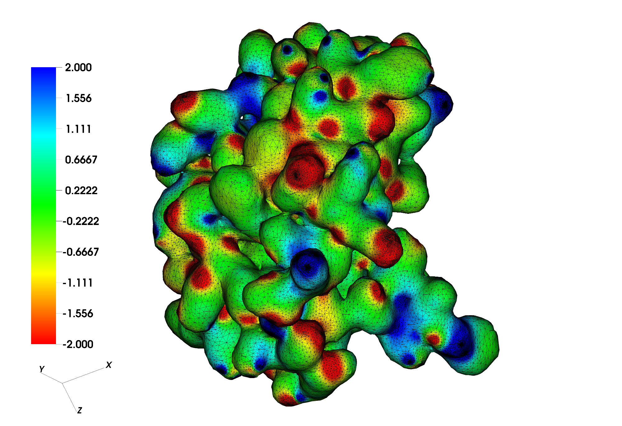
Figure 3: Full potential surface map of the insulin protein (PDB ID: 1RWE) in units $k_{B}T/e_{c}$. Blue color indicates a positive potential (values$>2k_{B}T/e_{c}$) and red color indicates negative potential (values $<-2K_{B}T/e_{c}$).

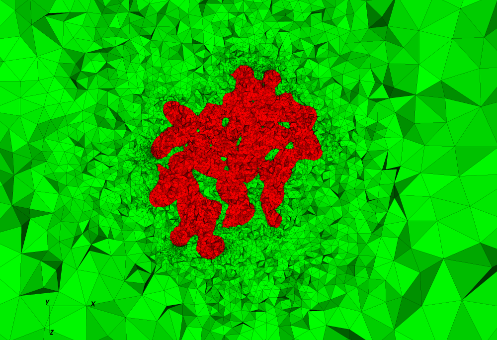
Figure 4: Cross section of the mesh with the plane $y=15\,\AA$ at level 2 in the mesh refinement procedure for finding the component $\tilde{u}^{N}$ in Example 2. The molecule region $\Omega_{m}$ is marked red.

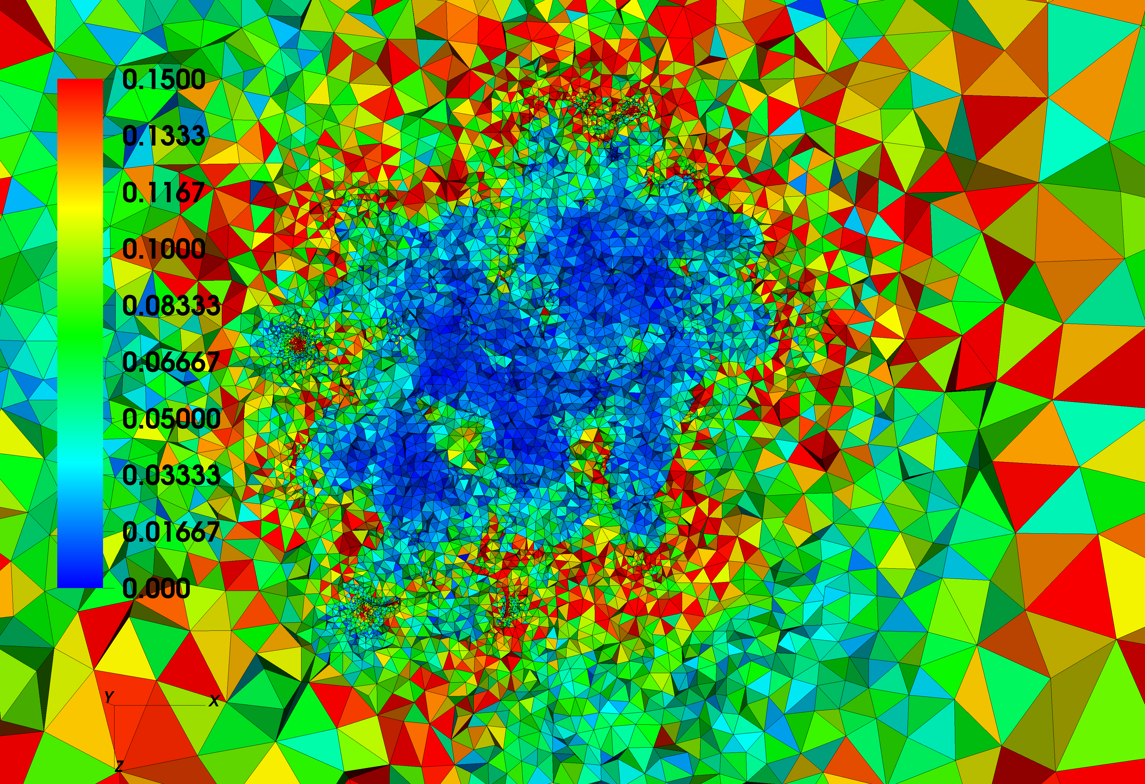
Figure 5: Cross section of the mesh with the plane $y=15\,\AA$ at level 2 in the mesh refinement procedure for finding the component $\tilde{u}^{N}$ in Example 2. Error indicator as a piecewise constant function.

4.4 Example 3: (Alexa 488 and Alexa 594) 3-term regularization without additional splitting in $u^{L}+u^{N}$

In this example, we solve the PBE for the system consisting of the two chromophores Alexa 488 and Alexa 594 but this time we utilize the 3-term regularization scheme without further splitting the regular component $u$ in $u^{L}+u^{N}$. The parameters are the same as in the first example, i.e., $\epsilon_{m}=2$, $\epsilon_{s}=80$, $k_{m}^{2}=0\,\AA^{-2}$, $k_{s}^{2}=10\,\AA^{-2}$ which corresponds to ionic strength $I_{s}\approx 1.178$ molar.

4.4.1 Finding the harmonic component $u^{H}$

According to the 3-term regularization, we first have to obtain a conforming approximation $\tilde{u}^{H}$ of $u^{H}$ by solving problem (2.14). We solve this problem on a sequence of adapted meshes using the error majornat (3.1) and the derived from it error indicator. To reconstruct the numerical flux $\nabla\tilde{u}^{H}$ and obtain $T(\nabla\tilde{u}^{H})$ we can either minimize the majorant (3.1) over a subspace of $H(\operatorname{div};\Omega_{m})$, like $RT_{0}$, or apply some patchwise flux reconstruction technique. We notice that minimization of the majorant over $RT_{0}$ defined on the same mesh and applying the patchwise equilibrated flux reconstruction from [6] yields practically the same results. We have computed $\tilde{u}^{H}$ on a final mesh with $20\,615\,534$ tetrahedrons. The corresponding value for the majorant in (3.1) is $M_{\oplus,H}\left(\tilde{u}^{H},T(\nabla\tilde{u}^{H})\right)=43.085$, where $T(\nabla\tilde{u}^{H})$ is obtained by the flux reconstruction in [6] and thus $\operatorname{div}\left(T(\nabla\tilde{u}^{H})\right)=0$. Since in this case $\|\nabla\left(\tilde{u}^{H}-u^{H}\right)\|_{L^{2}(\Omega_{m})}\leq M_{\oplus,H}\left(\tilde{u}^{H},T(\nabla\tilde{u}^{H})\right)=43.085$, we obtain a guaranteed upper bound on the relative error in energy norm

$$\frac{\|\nabla\left(\tilde{u}^{H}-u^{H}\right)\|_{L^{2}(\Omega_{m})}}{\|\nabla u^{H}\|_{L^{2}(\Omega_{m})}}\leq 3.16\,\%.$$

4.4.2 Finding the regular component $\tilde{u}$

Now, we find a conforming approximation $\tilde{u}_{h}\in V_{h}$ of $\tilde{u}$, the exact solution of problem (3.39), by adaptively solving the Galerkin problem (3.4), where $V_{h}\subset H_{0}^{1}(\Omega)$ is the $P_{1}$ Lagrange finite element space . By $\tilde{u}_{i}$ and $\tilde{y}^{*}_{i}$ we denote the finite element approximations at mesh refinement level $i$ to $\tilde{u}$ and $\tilde{p}^{*}$, respectively. Here $\bar{p}=6$. To find a good approximation $\tilde{y}^{*}$ of the exact flux $\tilde{p}^{*}$ of the form (3.17), i.e., $\tilde{y}^{*}$ such that

$$\tilde{y}^{*}=-\epsilon_{m}T(\nabla\tilde{u}^{H})\mathbbm{1}_{\Omega_{m}}+\epsilon_{m}\nabla G\mathbbm{1}_{\Omega_{s}}+\tilde{y}_{0}^{*},\text{ for }\tilde{y}_{0}^{*}\in H(\operatorname{div};\Omega)\text{ with }\operatorname{div}\tilde{y}_{0}^{*}=0\text{ in }\Omega_{m},$$

we can minimize the majorant $M^{2}_{\oplus}(\tilde{u},\tilde{y}^{*})$ or, equivalently, minimize the functional $-I^{*}(\tilde{y}^{*})=G^{*}(\tilde{y}^{*})+F^{*}(-\Lambda^{*}\tilde{y}^{*})$ in $\tilde{y}_{0}^{*}$ over a subspace of $H(\operatorname{div};\Omega)$, like $RT0,RT1$, by additionally enforcing the condition that $\operatorname{div}\tilde{y}_{0}^{*}=0$ in $\Omega_{m}$. Another, computationally favourable, approach, which can be easily realized in parallel, is to apply a patchwise flux reconstruction that will also yield $\operatorname{div}\tilde{y}_{0}^{*}=0$ in $\Omega_{m}$. Such an approach is motivated by observing that the exact $\tilde{p}_{0}^{*}:=\tilde{p}^{*}+\epsilon_{m}T(\nabla\tilde{u}^{H})\mathbbm{1}_{\Omega_{m}}-\epsilon_{m}\nabla G\mathbbm{1}_{\Omega_{s}}$ satisfies the integral identity

$$\int\limits_{\Omega}{\tilde{p}_{0}^{*}\cdot\nabla vdx}=-\int\limits_{\Omega}{k^{2}\sinh(\tilde{u})vdx},\text{ for all }v\in H_{0}^{1}(\Omega).$$ (4.17)

If we define the function $q:=\epsilon\nabla\tilde{u}_{h}+\epsilon_{m}T\left(\nabla\tilde{u}^{H}\right)\mathbbm{1}_{\Omega_{m}}-\epsilon_{m}\nabla G\mathbbm{1}_{\Omega_{s}}$, then we can see that

$$\int\limits_{\Omega}{q\cdot\nabla vdx}=-\int\limits_{\Omega}{k^{2}\sinh(\tilde{u}_{h})vdx},\text{ for all }v\in V_{h}.$$

Now, we define $\Pi_{L_{h}}(q)$ to be its $L^{2}$ projection over the space $L_{h}$ of piecewise constant functions over the same mesh on which $V_{h}$ is defined. Since $\Pi_{L_{h}}\left(q\right)$ satisfies the problem

$$\int\limits_{\Omega}{\Pi_{L_{h}}(q)\cdot\nabla vdx}=-\int\limits_{\Omega}{k^{2}\sinh(\tilde{u}_{h})vdx},\text{ for all }v\in V_{h},$$ (4.18)

we define $\tilde{y}_{0}^{*}\in RT_{0}$ by applying the patchwise equilibrated flux reconstruction in [6] to the numerical flux $\Pi_{L_{h}}(q)\in L_{h}$ . Notice that since $k=0$ in $\Omega_{m}$, the obtained $\tilde{y}_{0}^{*}$ satisfies the realtion $\operatorname{div}\tilde{y}_{0}^{*}=0$ in $\Omega_{m}$. We define in a similar fashion, as for the component $\tilde{u}^{N}$, the quantities ${\text{PRE}}_{i,i}^{\text{Up}}$, ${\text{RE}}_{i,j,k,s}^{\text{Up}}$, ${\text{RCEN}}_{i,j,s}^{\text{Low}}$, ${\text{P}}_{\text{rel},i}^{\text{CEN}}$, ${\text{RCEN}}_{i,j,s}^{\text{Up}}$.

Table 14: Example 3

Example 3: $k_{m}^{2}=0,\,k_{s}^{2}=10,\,\epsilon_{m}=2,\,\epsilon_{s}=80$
level $i$	#elements	$\|\tilde{u}_{i}\|_{0}$	${\left|\kern-0.96873pt\left|\kern-0.96873pt\left|\nabla\tilde{u}_{i}\right|\kern-0.96873pt\right|\kern-0.96873pt\right|}$	${\left|\kern-0.96873pt\left|\kern-0.96873pt\left|\epsilon\nabla\tilde{u}_{i}-\tilde{y}_{i}^{*}\right|\kern-0.96873pt\right|\kern-0.96873pt\right|}_{*}$	$\sqrt{2}M_{\oplus}(\tilde{u}_{i},\tilde{y}_{i}^{*})$	$\tilde{J}(\tilde{u}_{i})$
0	667 008	67.614	361.00	200.91	201.89	258854115.518
1	1 384 294	68.342	363.74	127.75	128.44	258852218.914
2	2 162 155	68.445	364.54	108.08	108.72	258851876.473
3	2 889 668	68.512	365.00	97.878	98.456	258851659.119
4	3 591 411	68.554	365.26	91.161	91.700	258851527.684
5	4 322 074	68.583	365.44	86.080	86.587	258851434.952
6	5 142 768	68.607	365.58	81.773	82.252	258851360.368
7	6 108 164	68.626	365.70	77.910	78.362	258851296.239
8	7 276 168	68.643	365.81	74.263	74.690	258851239.273
9	8 690 783	68.658	365.91	71.903	72.299	258851187.598
10	10 390 012	68.671	366.01	67.538	67.917	258851140.495
11	12 431 042	68.683	366.09	64.457	64.814	258851097.844
12	14 871 214	68.695	366.17	61.558	61.893	258851059.718

Table 15: Example 3

Example 3: $k_{m}^{2}=0,\,k_{s}^{2}=10,\,\epsilon_{m}=2,\,\epsilon_{s}=80$
level $i$	#elements	${\text{PRE}}_{i,i}^{\text{Up}}[\%]$	${\text{RE}}_{i,i,i,i}^{\text{Up}}[\%]$	${\text{RCEN}}_{i,i,i}^{\text{Low}}[\%]$	${\text{P}}_{\text{rel},i}^{\text{CEN}}[\%]$	${\text{RCEN}}_{i,i,i}^{\text{Up}}[\%]$
0	667 008	55.65	126.8	18.91	39.35	58.10
1	1 384 294	35.12	54.59	13.71	24.83	31.95
2	2 162 155	29.65	42.50	12.02	20.96	25.99
3	2 889 668	26.81	36.93	11.09	18.96	23.05
4	3 591 411	24.95	33.52	10.45	17.64	21.17
5	4 322 074	23.55	31.05	9.967	16.65	19.79
6	5 142 768	22.36	29.03	9.544	15.81	18.63
7	6 108 164	21.30	27.27	9.158	15.06	17.61
8	7 276 168	20.30	25.65	8.789	14.35	16.66
9	8 690 783	19.65	24.62	8.547	13.89	16.05
10	10 390 012	18.45	22.78	8.094	13.04	14.95
11	12 431 042	17.60	21.51	7.769	12.44	14.18
12	14 871 214	16.81	20.34	7.460	11.88	13.46

Table 16: Example 3

Example 3: $k_{m}^{2}=0,\,k_{s}^{2}=10,\,\epsilon_{m}=2,\,\epsilon_{s}=80$
level $i$	#elements	${\text{RE}}_{i,\bar{p},\bar{p},\bar{p}}^{\text{Up}}[\%]$	${\text{RCEN}}_{i,\bar{p},\bar{p}}^{\text{Low}}[\%]$	${\text{RCEN}}_{i,\bar{p},\bar{p}}^{\text{Up}}[\%]$	${\left|\kern-0.96873pt\left|\kern-0.96873pt\left|\epsilon\nabla\tilde{u}_{i}-\tilde{y}_{\bar{p}}^{*}\right|\kern-0.96873pt\right|\kern-0.96873pt\right|}_{*}$	$\sqrt{2}M_{\oplus}(\tilde{u}_{i},\tilde{y}_{\bar{p}}^{*})$
0	667 008	32.75	24.34	43.92	99.184	99.665
1	1 384 294	25.75	15.48	27.94	78.070	78.374
2	2 162 155	24.27	13.09	23.65	73.546	73.857
3	2 889 668	23.28	11.86	21.41	70.520	70.840
4	3 591 411	22.66	11.04	19.94	68.630	68.957
5	4 322 074	22.21	10.43	18.83	67.274	67.607
6	5 142 768	21.85	9.910	17.89	66.170	66.507
7	6 108 164	21.54	9.442	17.04	65.209	65.550
8	7 276 168	21.26	9.000	16.24	64.348	64.692
9	8 690 783	21.00	8.714	15.72	63.564	63.910
10	10 390 012	20.76	8.185	14.77	62.843	63.191
11	12 431 042	20.54	7.811	14.10	62.179	62.525
12	14 871 214	20.34	7.460	13.46	61.558	61.893

We should note that the bounds on the error in energy norm obtained by the majorant $\sqrt{2}M_{\oplus}(\tilde{u}_{i},\tilde{y}_{i}^{*})$ in Table 14 are rather conservative and they could be improved by applying a flux reconstruction involving a higher order Raviart-Thomas spaces, like $RT_{1}$. To obtain an idea of how much the error is overestimated, we can compare the values $\sqrt{2}M_{\oplus}(\tilde{u}_{0},\tilde{y}^{*}_{\bar{p}})$ and $\sqrt{2}M_{\oplus}(\tilde{u}_{1},\tilde{y}^{*}_{\bar{p}})$ of the majorant, evaluated with the last available approximation $\tilde{y}^{*}_{\bar{p}}$ of the exact flux $\tilde{p}^{*}$ to the values $\sqrt{2}M_{\oplus}(\tilde{u}_{0},\tilde{y}^{*}_{0})$ and $\sqrt{2}M_{\oplus}(\tilde{u}_{1},\tilde{y}^{*}_{1})$ evaluated with the current $\tilde{y}^{*}_{0}$ and $\tilde{y}^{*}_{1}$ at the first two meshes. We see that the overestimation is between around $201.89/99.665\approx 2.025$ and $128.44/78.374\approx 1.64$ times. This means that it is safe to assume that the real error ${\left|\kern-1.07639pt\left|\kern-1.07639pt\left|\nabla(\tilde{u}-\tilde{u}_{12})\right|\kern-1.07639pt\right|\kern-1.07639pt\right|}$ at the last level $\bar{p}=12$ is no more than approximately $\sqrt{2}M_{\oplus}(\tilde{u}_{\bar{p}},\tilde{y}^{*}_{\bar{p}})/2\approx 31$. With this in mind, we can obtain an overall guaranteed bound on the error in energy norm for the regular component $u$ by using (3.41):

$$\mathrel{\phantom{=}}{\left|\kern-1.07639pt\left|\kern-1.07639pt\left|\nabla(u-\tilde{u}_{h})\right|\kern-1.07639pt\right|\kern-1.07639pt\right|}\leq\sqrt{\epsilon_{m}}M_{\oplus,H}\left(\tilde{u}^{H},T(\nabla\tilde{u}^{H})\right)+\sqrt{2}M_{\oplus}(\tilde{u}_{h},\tilde{y}^{*})$$

$$=\sqrt{2}\times 43.085+61.893=122.824$$

Figure 6: Full potential surface map with the 3-term regularization (without additional splitting into $u^{L}+u^{N}$) for the system Alexa 488 and Alexa 594 in units $k_{B}T/e_{c}$. Blue color indicates a positive potential (values$>2.5k_{B}T/e_{c}$) and red color indicates negative potential (values $<-2.5K_{B}T/e_{c}$).

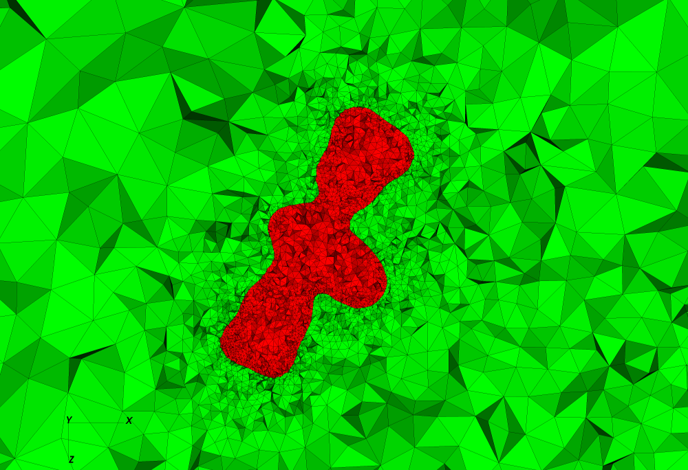
Figure 7: Cross section of the mesh with the plane $y=3\,\AA$ at level 1 in the mesh refinement procedure for finding the component $\tilde{u}$ in Example 3. The molecule region $\Omega_{m}$ is marked red (Alexa 594).

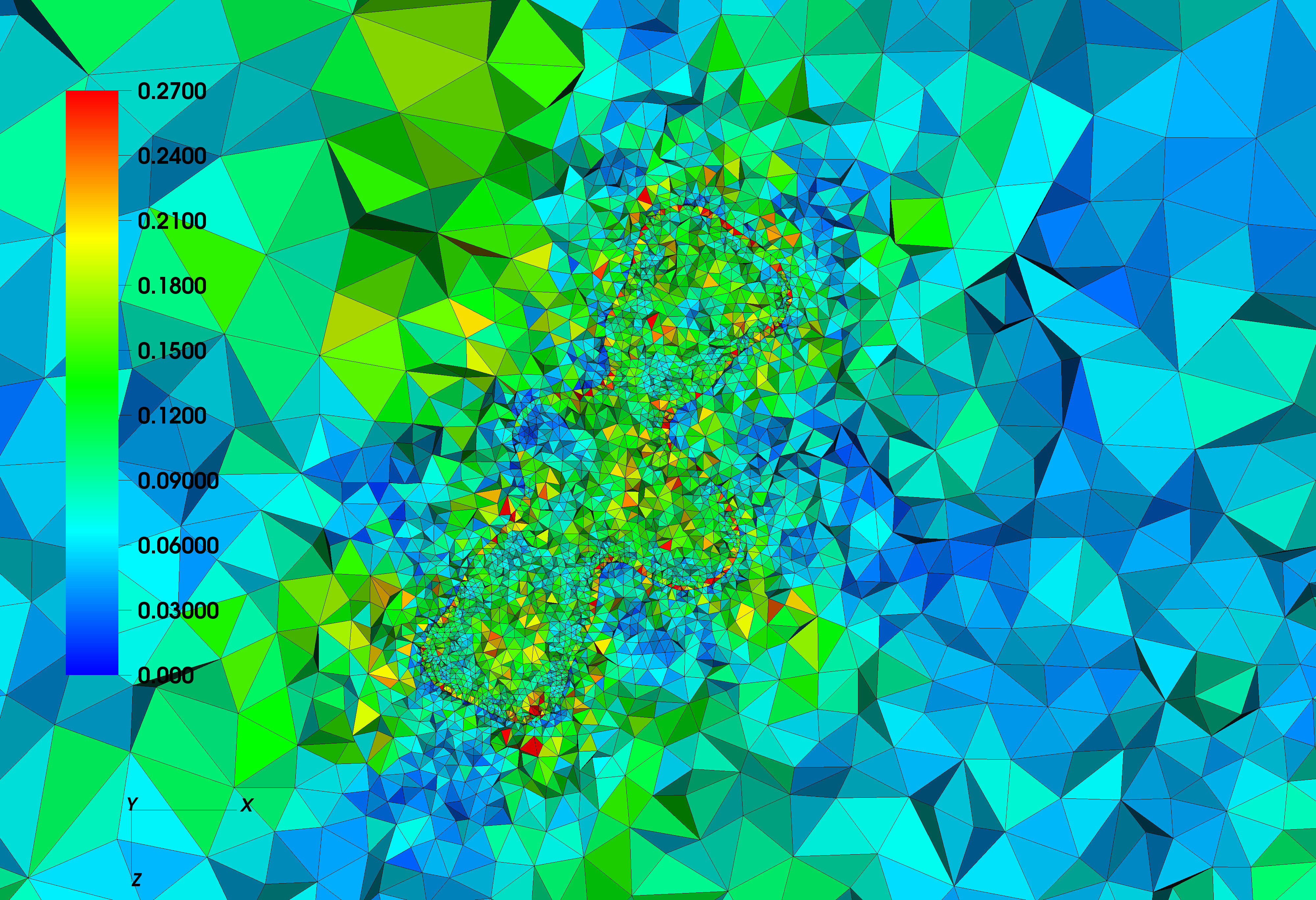
Figure 8: Cross section of the mesh with the plane $y=3\,\AA$ at level 1 in the mesh refinement procedure for finding the component $\tilde{u}$ in Example 3. Error indicator as a piecewise constant function.

5 Conclusions

We have analyzed the well posedness of two and three-term regularization schemes for the Poisson-Boltzmann equation and derived guaranteed and fully computable bounds on the error in energy norm. For the 2-term regularization the dimensionless potential $\tilde{\phi}$ is decomposed into $G+u$ where $G$ is analytically known and $u\in H^{1}(\Omega)$ is the regular component which has to be approximated, that is, computed numerically. The regular component $u$ can be split additionally into $u^{L}+u^{N}$ where $u^{L}$ solves a linear nonhomogeneous interface problem and $u^{N}$ solves a nonlinear homogeneous problem which depends on $u^{L}$. For each of these two problems we have derived guaranted bounds on the error in energy norm. Moreover, for the nonlinear problem, we have proved a continous dependence of the solution $u^{N}$ on perturbations in $u^{L}$. This property has been exploited to estimate the overall error in the regular component $u$. The derived error estimate for $u$ is a linear combination of the majorants for the error in $u^{L}$ and the error in $u^{N}$ with perturbed $u^{N}$. Similarly, in the 3-term regularization scheme, the dimensionless potential $\tilde{\phi}$ is decomposed into $G+u^{H}+u$. Here $u^{H}\in H^{1}(\Omega)$ is a harmonic function in the molecular domain $\Omega_{m}$, which has to be approximated numerically, and is equal to $-G$ in the solution domain $\Omega_{s}$. Now, the regular component $u$ satisfies a nonlinear nonhomogeneous interface problem which depends on $u^{H}$. To solve this problem, we have analyzed two approaches. The first is to additionally make the splitting $u=u^{L}+u^{N}$ as we did in case of the 2-term regularization. In this case, we have analyzed how $u^{L}$ depends on perturbations in $u^{H}$, and further, how $u^{N}$ depends on perturbations in $u^{L}$. Finally, we have derived an estimate for the overall error in the regular component $u$, which is a linear combination of the majorants for the error in each of the components $u^{H},u^{L}$, and $u^{N}$. The second approach to derive estimates for the regular component $u$ of the solution of the nonlinear interface problem is to directly derive an error estimate for it and analyze its continuous dependence on perturbations in $u^{H}$. In this case, the overall estimate for the error in energy norm is a linear combination of the majorants for the error in $u^{H}$ and the error in $u$ with perturbed $u^{H}$.

The a posteriori error analysis presented in this paper is based on the functional approach developed in [31]. We have also utilized this approach to obtain a near best approximation result for the two regularization schemes which is the basis for the analysis of qualified and unqualified convergence of finite element approximations. In other words, the generality of this method allows for the derivation of both a posteriori and a priori error estimates for the considered class of problems.

We have presented three numerical tests performed on two realistic physical systems illustrating and validating our theoretical findings. The first system consists of the two chromophores, Alexa 488 and Alexa 594, and the second system of an insulin protein with a PDB ID 1RWE. The guaranteed error bounds which we have derived do not overestimate the error as drastically as residual based error estimates often do. To obtain a conforming approximation of the dual variable, we have utilized a patchwise flux reconstruction technique, cf. [6], which can be easily implemented on parallel machines by a scalable algorithm with linear complexity. This means that the proposed error estimation can be realized in a very efficient manner.

References

• [1] B. Lu, Y. Zhou, M. Holst, J. McCammon. Recent progress in numerical methods for the Poisson-Boltzmann equation in biophysical applications. Commun. Comput. Phys., 3(5):973–1009, 2008.
• [2] J. Buse. Insulin analogues. Curr. Opin. Endocrinol. Diabetes, 8:95–100, 2001.
• [3] M. Chen, B. Tu, and B. Lu. Triangulated manifold meshing method preserving molecular surface topology. J. Mol. Graph. Model., 38:411–418, 2012.
• [4] Hank Childs, Eric Brugger, Brad Whitlock, Jeremy Meredith, Sean Ahern, David Pugmire, Kathleen Biagas, Mark Miller, Cyrus Harrison, Gunther H. Weber, Hari Krishnan, Thomas Fogal, Allen Sanderson, Christoph Garth, E. Wes Bethel, David Camp, Oliver Rübel, Marc Durant, Jean M. Favre, and Paul Navrátil. VisIt: An End-User Tool For Visualizing and Analyzing Very Large Data. In High Performance Visualization–Enabling Extreme-Scale Scientific Insight, pages 357–372. Oct 2012.
• [5] Paolo Cignoni, Marco Callieri, Massimiliano Corsini, Matteo Dellepiane, Fabio Ganovelli, and Guido Ranzuglia. MeshLab: an Open-Source Mesh Processing Tool. In Vittorio Scarano, Rosario De Chiara, and Ugo Erra, editors, Eurographics Italian Chapter Conference. The Eurographics Association, 2008.
• [6] D. Braess, J. Schöberl. Equilibrated residual error estimator for Maxwell’s equations. RICAM report, 2006.
• [7] D. Chapman. A contribution to the theory of electrocapillarity. Phil. Mag., 25:475–481, 1913.
• [8] D. Kinderlehrer, G. Stampacchia. An Introduction to Variational Inequalities and Their Applications. SIAM, 2000.
• [9] C. Dapogny, C. Dobrzynski, and P. Frey. Three-dimensional adaptive domain remeshing, implicit domain meshing, and applications to free and moving boundary problems. Technical report, March 2013.
• [10] Cecile Dobrzynski. MMG3D: User Guide. Technical Report RT-0422, INRIA, March 2012.
• [11] F. Fogolari, A. Brigo, H. Molinari. The Poisson-Boltzmann equation for biomolecular electrostatics: a tool for structural biology. J. Mol. Recognit., 15:377–392, 2002.
• [12] G. Gouy. Constitution of the electric charge at the surface of an electrolyte. J. Phys., 9:457–468, 1910.
• [13] H. Oberoi, N. M. Allewell. Multigrid solution of the nonlinear Poisson-Boltzmann equation and calculation of titration curves. Biophysical Journal, 65:48–55, 1993.
• [14] F. Hecht. New development in FreeFem++. J. Numer. Math., 20(3-4):251–265, 2012.
• [15] I. Ekeland, R. Temam. Convex Analysis and Variational Problems. North-Holland Publishing Company, 1976.
• [16] J. Elschner, J. Rehberg, G. Schmidt. Optimal regularity for elliptic transmission problems including C1 interfaces. Interfaces and Free Boundaries, 9(2):233–252, 2007.
• [17] J. Kirkwood. Theory of solutions of molecules containing widely separated charges with special applications to zwitterions. J. Chem. Phys., 7:351–361, 1934.
• [18] J. Li, S. Wijeratne, X. Qiu, and C.-H. Kiang. DNA under force: Mechanics, electrostatics, and hydration. Nanomaterials, 5(1):246–267, 2015.
• [19] J. Lipfert, S. Doniach, R. Das, and D. Herschlag. Understanding nucleic acid-ion interactions. Annu Rev Biochem., 83:813–841, 2014.
• [20] K. A. Sharp, B. Honig. Calculating total electrostatic energies with the nonlinear Poisson-Boltzmann equation. J. Phys. Chem, 94:7684–7692, 1990.
• [21] J. Kraus, S. Nakov, and S. Repin. Reliable numerical solution of a class of nonlinear elliptic problems generated by the Poisson-Boltzmann equation. arXiv, 2018.
• [22] T. Liu, M. Chen, and B. Lu. Efficient and qualified mesh generation for Gaussian molecular surface using adaptive partition and piecewise polynomial approximation. SIAM J. Sci. Comput, 40:507–527, 2018.
• [23] Long Chen, Michael J. Holst, Jinchao Xu. Adaptive finite element modeling techniques for the Poisson-Boltzmann equation. Siam J. Numer. Anal., 45(6):2298–2320, 2007.
• [24] M. Gilson, M. Davis, B. Luty and J. McCammon. Computationn of electrostatic forces on solvated molecules using the poisson-boltzmann equation. J. Phys. Chem., 97:3591–3600, 1993.
• [25] M. Holst, J.A. McCammon, Z. Yu, Y. C. Zhou, Y. Zhu. Adaptive finite element modeling techniques for the Poisson-Boltzmann equation. Commun. Comput. Phys., 11:179–214, 2012.
• [26] S. Mikhlin. Constants in Some Inequalities of Analysis. Chichester ; Wiley. Translated by Reinhard Lehmann, 1986.
• [27] P. Debye and E. Huckel. Zur theorie der elektrolyte. Phys. Zeitschr., 24:185–206, 1923.
• [28] P. Grisvard. Elliptic Problems in Nonsmooth Domains. Pitman Advanced Publishing Program, 1985.
• [29] P. Neittaanmaki, S. Repin. Reliable Methods for Computer Simulation: Error Control and Posteriori Estimates. Elsevier, 2004.
• [30] S. Repin. On measures of errors for nonlinear variational problems. Russian J. Numer. Anal. Math. Modelling, 27(6):577–584, 2012.
• [31] S. Repin. A posteriori error estimation for variational problems with uniformly convex functionals. Math. Comp, 69:481–500, 2000.
• [32] S. Repin. A Posteriori Estimates for Partial Differential Equations. Walter de Gruyter‘, 2008.
• [33] H. Si. TetGen, a Delaunay-based quality tetrahedral mesh generator. ACM Transactions on Mathematical Software (TOMS), 41(11), 2015.
• [34] E. Sobakinskaya, M. Schmidt am Busch, and T. Renger. Theory of FRET ”spectroscopic ruler” for short distances: Application to polyproline. J. Phys. Chem. B, 112:54–67, 2018.
• [35] Z. Wan et al. Enhancing the activity of insulin at the receptor interface: crystal structure and photo-cross-linking of A8 analogues. Biochemistry, 43:16119–16133, 2004.
• [36] Z.-J. Tan and S.-J. Chen. Predicting electrostatic forces in RNA folding. Methods Enzymol., 469:465–487, 2009.