Spectrum management and compatibility studies with Python

Abstract

We developed the pycraf Python package, which provides functions and procedures for various tasks related to spectrum-management compatibility studies. This includes an implementation of ITU-R Rec. P.452, which allows to calculate the path attenuation arising from the distance and terrain properties between an interferer and the victim service. A typical example would be the calculation of interference levels at a radio telescope produced from a radio broadcasting tower. Furthermore, pycraf provides functionality to calculate atmospheric attenuation as proposed in ITU-R Rec. P.676.

Using the rich ecosystem of scientific Python libraries and our pycraf package, we performed a large number of compatibility studies. Here, we will highlight a recent case study, where we analysed the potential harm that the next-generation cell-phone standard 5G could bring to observations at a radio observatory. For this we implemented a Monte-Carlo simulation to deal with the quasi-statistical spatial distribution of base stations and user devices around the radio astronomy station.

TODO

The electromagnetic spectrum, especially at radio frequencies, is a limited resource, which has tremendous economic and scientific value for a large variety of services. Applications involve mobile communication networks, radio and TV broadcasting, RADAR, and safety distress signals. In contrast, natural sciences such as radio astronomy, Earth sensing (which is important for climatology), or weather forecasting rely heavily on interference-free spectral bands to conduct measurements with their high-sensitivity receivers. Especially, the radio-astronomy service (RAS) developed receivers, often cryogenically cooled, that allow us to detect even the faintest signals from outer space. Today it is possible to observe Micro-Jansky sources, with a Jansky (Jy) being a unit of the spectral power flux density, which was introduced to honour Karl. G. Jansky the “founder” of the radio-astronomy field. It is $1\leavevmode\nobreak\ \mathrm{Jy}=10^{-26}\leavevmode\nobreak\ \mathrm{W}\,\mathrm{m}^{-2}\,\mathrm{Hz}^{-1}$.

With the increased utilization of the radio spectrum, it became essential to regulate its usage. Allocations of frequency bands are nowadays made by the International Telecommunication Union Radiocommunication Sector (ITU-R) in unanimous decisions by delegates of the administrations of its member states. Every two to four years, ITU-R organizes the World Radiocommunication Conference (WRC) where the so-called Radio Regulations are updated, which contain rules and procedures, and spectrum allocation tables. It is clear that such decisions and allocations have to be made in accordance to the technical needs and constraints of the concerned services. Therefore, in many regional and international organizations and institutions compatibility studies are performed, which analyse if, and possibly under which restrictions, a service can be granted a new allocation.

In the following, we present a new Python library, called pycraf, that can be used to carry out many of the recurring tasks, which occur in compatibility studies. This includes the estimation of path propagation losses and atmospheric dampening effects, the determination of satellite positions (given orbital parameters), or calculating antenna gain patterns. After a short introduction into compatibility studies in Section 1, the more important pycraf features are briefly introduced in Section 2.1 along with basic usage examples. A real-world application is discussed in Section 3, where the potential impact of the next-generation 5G mobile communication networks, which may acquire a new allocation at 24 GHz at the upcoming WRC-19, on the RAS is studied. Conclusions are presented in Section 3.6.

1 Spectrum management and compatibility studies

Many compatibility studies follow a very simple recipe. The first step is usually to calculate the radiated power (or the power flux density), $P_{\mathrm{tx}}$, at the transmitter (Tx). Then one has to determine the appropriate interference threshold for the detected power, $P_{\mathrm{rx}}$, at the victim receiver (Rx). The ratio $P_{\mathrm{tx}}/P_{\mathrm{rx}}$ constitutes the minimum shielding between interfering Tx and victim Rx, also called “minimum coupling loss” (MCL). In the final step the product of antenna gains and the path propagation loss (or path attenuation), i.e., the loss of power on the path to the receiver (Rx) is determined and compared to the MCL. That way one may find the minimum distance between a single interferer and victim receiver, which is often called separation distance. Since the path propagation loss also depends on the terrain height profile between Tx and Rx, the necessary separation distance will vary for different bearings, leading to non-circular exclusion zones around a victim receiver. In the case of a widespread deployment of many possible interferers one may need to calculate the expected total (“aggregated”) interference levels from all interferers within a certain range around the victim receiver. In most cases this will require a statistical simulation of possible deployments in a given terrain. However, simplified numerical convolutions of path loss laws with the deployment distribution functions are often cheaper to compute and can also yield good estimates of the size of zones where interferers ought to be excluded.

1.1 Available software

The various tasks that have to be solved in typical compatibility studies are often similar. Nevertheless, major effort is necessary to develop a single tool, which could be used in all sorts of different scenarios.

One such tool is Seamcat (ECC Report 252), which was developed by the European Communications Committee (ECC) to be used by spectrum managers in CEPT countries. It lets the user choose from a large amount of system parameters, deployment scenarios, and path propagation models – all with appropriate distribution functions – and applies Monte-Carlo sampling to calculate the desired output distributions, e.g., of the power levels detected at a receiver. Unfortunately, as of today, Seamcat can only perform so-called generic studies, i.e., the terrain profile between a transmitter and receiver is either neglected or approximated in a very coarse manner. For RAS stations in mountainous terrain this may lead to unrealistic results as the diffraction at hill or mountain tops can significantly increase the path attenuation between victim and interferer(s).

PathProfile is a publicly available software tool for the prediction of local field strengths developed by Mike Willis. It features a GUI and uses terrain data for the calculation of path loss. As such, it may serve as the core of compatibility calculations, but will require additional specific interfacing for multi-interferer scenarios or aggregation studies.

A variety of MATLAB-based solutions to various spectrum management problems exists and is used by regulatory administrations, industry, and also by radio astronomers in spectrum management. Some of them have found approval by the ECC (e.g. ECC Report 247, ), but many are not in the public domain and less well known and are used mainly by individuals.

2 The pycraf package

While there are some existing software tools to aid with compatibility studies, they are either not suited for all relevant tasks (PathProfile), not easy to use from within a programming language (Seamcat), or are based on proprietary software (MATLAB-based scripts). Therefore, we decided to provide a number of functions and procedures, which were developed in the framework of several radio compatibility studies involving the Effelsberg observatory. The observatory is located in the Eifel mountains in Western Germany and operates a 100-m radio telescope. The code comes in the form of a Python library (a so-called package) that can easily be installed and used even by relatively inexperienced Python users. The package is named pycraf, open-source licensed (GPL-v3), and available on the Python package distribution server PyPI (Python Package Index. The source code is furthermore hosted on the GitHub platform, along with detailed documentation, a bug tracker, and installation instructions.

We aim to make pycraf a community-driven project. Contributions to the source code or documentation are very welcome, but we are also happy to receive bug reports, feature requests and other proposals that would further improve the package.

The pycraf package makes use of the AstroPy package template providing a sophisticated build environment, which is based on setuptools, pytest, and sphinx. It allows the use of automated testing, makes incorporation of continuous integration services easy, and enables automated documentation generation. Because pycraf is available on the PyPI distribution server, one can use the Python tool pip to install the package into the local Python environment.

After successful installation, one can load and test the library with the following two statements:

⬇

import pycraf

pycraf.test(remote_data=’any’)

With this remote_data option, pycraf will attempt to download terrain-height data from the NASA Shuttle Radar Topography Mission (SRTM Farr et al., 2007) for the calculation of path propagation loss in real terrain.

In the following we will present an overview of the features included in pycraf and provide some basic examples for its use. A discussion of all aspects of pycraf and introduction to the various third-party libraries used in pycraf is beyond the scope of this paper and we refer to the online manual where a lot more information and a full API reference for each sub-package can be found. We also note that pycraf makes extensive use of the Astropy (physical) units module, which is well documented on the Astropy website.

2.1 Conversions module

Most of the fundamental operations, e.g., converting the radiated total power into an equivalent power flux density at a given distance and assuming a certain antenna gain of the Tx, or calculating the total received power at an Rx from the power flux density, are covered by the conversions sub-package. Furthermore, several Decibel units are defined, e.g.:

Listing 1: Conversions module.

⬇

1import astropy.units as u

2import pycraf.conversions as cnv

3

4power = 1 * u.W

5

6print(’{:.2f}’.format(power))

7# 1.00 W

8

9print(’{:.2f}’.format(power.to(cnv.dB_W)))

10# 0.00 dB(W)

11

12print(’{:.2f}’.format(power.to(cnv.dBm)))

13# 30.00 dB(mW)

To calculate the power flux density (in vacuum) produced by a 1-W Tx at a distance of e.g. 1 km, assuming a forward antenna gain of 25 dBi and free-space propagation, one can use the function powerflux_from_ptx:

⬇

2p_tx = 1 * u.W

3gain_tx = 25 * cnv.dBi

4distance = 1 * u.km

5

6pfd = cnv.powerflux_from_ptx(

7 p_tx, distance, gain_tx

8 )

9

10print(’{:.2e}’.format(pfd))

11# 2.52e-05 W / m2

12

13print(’{:.2f}’.format(

14 pfd.to(cnv.dB_W_m2)

15 ))

16# -45.99 dB(W / m2)

Likewise, if such power flux density is received by an isotropic antenna, one can calculate the total received power (which depends on frequency):

⬇

13gain_rx = 0 * cnv.dBi

14frequency = 1 * u.GHz

15

16p_rx = cnv.prx_from_powerflux(

17 pfd, frequency, gain_rx

18 )

19

20print(’{:.2e}’.format(p_rx))

21# 1.80e-07 W

22

23print(’{:.2f}’.format(p_rx.to(cnv.dB_W)))

24# -67.45 dB(W)

The difference between Tx and Rx power for isotropic antennas is also called the free-space loss and can be calculated using Friis’ transmission equation:

⬇

16fspl = cnv.free_space_loss(

17 distance, frequency

18 )

19

20print(’{:.2f}’.format(fspl))

21# -92.45 dB

This result is consistent with the above approach, if the additional Tx antenna gain of 25 dBi is considered.

The conversions sub-package offers a lot more and we refer to the online documentation for a detailed overview of the functionality.

2.2 Path attenuation

The largest part of the code base is currently dedicated to the implementation of the path propagation loss algorithm described in ITU-R Rec. P.452. As discussed in Section 1, the path attenuation calculation is one of the three fundamental steps in any compatibility study. Furthermore, it is the most critical aspect, as the losses can easily exceed 100 dB and typically uncertainties are large. The method in P.452 includes various effects that influence the path loss:

1. Line-of-sight (free-space) loss including correction terms for multipath and focussing effects,
   

2. Diffraction (at terrain features),
   

3. Tropospheric scatter, and
   

4. Anomalous propagation (ducting, reflection from elevated atmospheric layers).

Furthermore, a simple correction is provided to include additional losses caused by local obstacles (“clutter”) at the end points of the propagation path. The details of the individual mechanisms are beyond the scope of this paper and we refer to the P.452 and references therein for further information.

We note, however, that the diffraction calculation was revised in version 15 of the P.452. Previously, it used the 3-edge Deygout method, while the new algorithm is based on the so-called delta-Bullington method. Because this change can significantly affect the results of the diffraction loss in mountainous terrain (see Wilson and Salamon, 2008, and references therein), pycraf offers both methods, from the older version 14 and the current version 16, such that one can compare older study results with the predictions of the new method.

While most of pycraf is pure Python code, for performance reasons the pathprof sub-package contains a large amount of Cython code (Behnel et al., 2011). Even then, the P.452 algorithm is computationally demanding and if one wants to create a large map of path attenuations around a transmitter, the calculation would be relatively slow. Allowing for an insignificant loss of numerical accuracy, we developed a fast alternative for this use case, which is presented in Section 2.2.1.

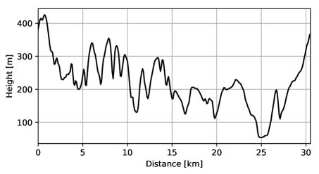
Figure 1: Example height profile as obtained with the program in Listing 2. Based on NASA SRTM data (Farr et al., 2007).

Before the path propagation loss can be calculated, a terrain height profile has to be constructed from a suitable data source. The pycraf package has built-in access to SRTM data servers, which allows to obtain so-called tiles ($1^{\circ}\times 1^{\circ}$) on demand:

Listing 2: Path profile module.

⬇

1import astropy.units as u

2import pycraf.conversions as cnv

3import pycraf.pathprof as pp

4

5# allow download of missing SRTM data:

6pp.SrtmConf.set(download=’missing’)

7

8lon_t, lat_t = (6.9, 50.5) * u.deg

9lon_r, lat_r = (7.3, 50.6) * u.deg

10step = 100 * u.m

11

12(

13 lons, lats, dist, dists, heights,

14 bearing, bbearing, bbearings

15 ) = pp.srtm_height_profile(

16 lon_t, lat_t, lon_r, lat_r, step

17 )

Of course, it is also possible to provide SRTM tiles in a local directory to avoid excessive network traffic. The returned variables contain the geographical longitudes and latitudes of the path, the distances and back-bearings of each point on the path with respect to the transmitter (which are inferred via Vincenty’s formulae for the Earth ellipsoid; Vincenty, 1975), as well as the heights (above the WGS84 mean sea level). Here, the code to plot the data is omitted, but Fig. 1 displays the result.

It is noted, however, that the relevant pycraf functions can query SRTM data automatically; users do not necessarily need to provide the height profile themselves. Calculating the propagation loss between two points is a two-step process. First, an auxiliary object, PathProp, is constructed that contains the geometrical, environmental, and terrain parameters necessary for the further calculations:

⬇

21frequency = 1 * u.GHz

22omega = 0 * u.percent

23temperature = 290 * u.K

24pressure = 1013 * u.hPa

25time_percent = 2 * u.percent

26h_tg, h_rg = (5, 50) * u.m

27

28zone_t = pp.CLUTTER.URBAN

29zone_r = pp.CLUTTER.SUBURBAN

30

31pprop = pp.PathProp(

32 frequency,

33 temperature, pressure,

34 lon_t, lat_t,

35 lon_r, lat_r,

36 h_tg, h_rg,

37 step,

38 time_percent,

39 zone_t=zone_t, zone_r=zone_r

40 )

Here, omega, is the fraction of the path that is over sea, time_percent is the percentage of time for which the propagation losses will be larger than the returned values (see P.452 for details), and $h_{\mathrm{tg,rg}}$ are the antenna heights of the Tx and Rx over ground, respectively. Furthermore, the clutter zone type can be specified for both end points.

The next step consists of feeding the PathProp instance into a function loss_complete

⬇

17# account for additional antenna gains

18G_t, G_r = (20, 15) * cnv.dBi

19

20tot_loss = pp.loss_complete(

21 pprop, G_t, G_r

22 )

23for l in tot_loss:

24 print(’{:.2f}’.format(l))

25# 122.34 dB

26# 149.94 dB

27# 181.99 dB

28# 162.70 dB

29# 149.94 dB

30# 169.15 dB

31# 134.15 dB

The returned Python tuple contains

1. $L_{\mathrm{bfsg}}$, the free-space loss,
   

2. $L_{\mathrm{bd}}$, the basic transmission loss caused by diffraction,
   

3. $L_{\mathrm{bs}}$, the tropospheric scatter loss,
   

4. $L_{\mathrm{ba}}$, the ducting/layer reflection loss,
   

5. $L_{\mathrm{b}}$, the complete path propagation loss,
   

6. $L_{\mathrm{b,corr}}$, as $L_{\mathrm{b}}$ but with clutter correction, and
   

7. $L$, as $L_{\mathrm{b}}$ but with clutter and gain correction.

An important property of the total propagation loss ($L_{\mathrm{b}}$ and $L$) is that it is not simply the product (or sum, if logarithmic representation is used) of the components. Again, we refer to P.452 for more details. To give the reader an impression on how the various quantities behave as a function of distance from the transmitter, we have calculated the components for each point in the terrain height profile (Fig. 1) and display them in Fig. 2. In contrast to the two-point calculation above, the antenna gains were neglected, as the effective gain towards each point along the path differs somewhat due to the different elevation angles of the path at the two stations. That however requires accounting for the respective antenna patterns, which is supported by pycraf, but beyond the scope of this simple example.

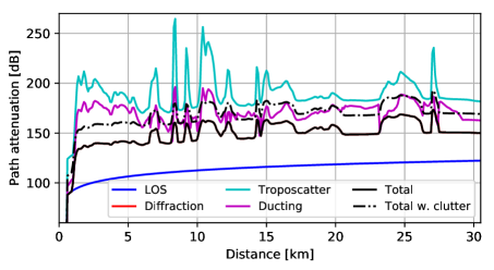
Figure 2: Path propagation loss along the terrain height profile displayed in Fig. 1. Based on NASA SRTM data (Farr et al., 2007).

2.2.1 A fast map-making algorithm

With the above approach it is straightforward to produce a path loss map, e.g., around a given transmitter, by simply calculating the propagation loss between each pixel in the map and the Tx location. As the P.452 algorithm is relatively complex, this would however require a substantial amount of computing time. In addition, the construction of the geodesics (the shortest paths between two points on the Earth ellipsoid) and SRTM height profile extraction/interpolation are also computationally demanding. Thus, two additional techniques were introduced to provide a significant speed-up. First, the map computation was moved into the Cython part of the code (avoiding the use of slower Python for-loops), where it is furthermore possible to make use of OpenMP for automatic parallelisation of the code to improve execution times on machines with many CPU cores. The second improvement is algorithmic in nature and aims to speed-up the geometric part of the computation: the geodesics calculation and height profile generation, which is preparatory work before the actual P.452-algorithm is employed. A path from the map centre to a pixel on the edge of the map crosses many other pixels in-between. We calculate all geodesics between map edge pixels and the centre and use a caching technique to identify the edge-geodesic which comes closest to the pixel centre for each interior pixel. This essentially transforms the problem from $O(n^{2})$ to $O(n)$. Unfortunately, the P.452 algorithm itself can not be treated with a similar technique, because the path elevation angles (and thus also if a path is line-of-sight or trans-horizon) are unique for each pixel as they depend on the terrain height profile between the pixel and the map centre.

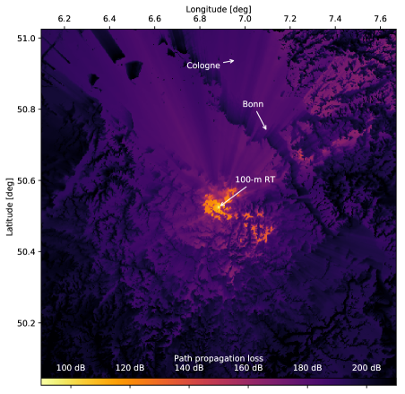
Figure 3: Example map of path propagation losses around the Effelsberg observatory. Based on NASA SRTM data (Farr et al., 2007).

Using the attenuation map-making functionality is again a two-step process. First, a helper object is created that caches the terrain and path parameters, which is then fed into the P.452 algorithm:

Listing 3: Fast path propagation loss map-making.

⬇

1import astropy.units as u

2import pycraf.conversions as cnv

3import pycraf.pathprof as pp

4

5pp.SrtmConf.set(download=’missing’)

6

7# Effelsberg radio telescope site

8lon_rt = 6.88361 * u.deg

9lat_rt = 50.52483 * u.deg

10

11# Map parameters

12msize_lon, msize_lat = (1, 1) * u.deg

13map_resolution = 3 * u.arcsec

14zone_t = pp.CLUTTER.URBAN

15zone_r = pp.CLUTTER.SUBURBAN

16

17# P.452 parameters

18frequency = 10 * u.GHz

19temperature = 290 * u.K

20pressure = 1013 * u.hPa

21time_percent = 2 * u.percent

22h_rt, h_tx = (50, 20) * u.m

23

24

25hprof_cache = pp.height_map_data(

26 lon_rt, lat_rt,

27 msize_lon, msize_lat,

28 map_resolution=map_resolution,

29 zone_t=zone_t, zone_r=zone_r,

30 )

31

32results = pp.atten_map_fast(

33 frequency,

34 temperature,

35 pressure,

36 h_rt, h_tx,

37 time_percent,

38 hprof_cache,

39 )

40

41total_atten = results[’L_b’]

Again, we omit the lengthy plot code, but the result of this is visualized in Fig. 3. The hprof_cache object is a Python dict-like object containing the cached parameters and could also be edited by the user before calling atten_map_fast. A typical example of such editing would be the assignment of a different clutter zone to each of the pixels – given that the user has access to a suitable database containing the true clutter types.

The pathprof sub-package also provides a large amount of other utility functions, e.g., to plot terrain maps or export maps to a Geographic Information System (GIS) file format such as the Keyhole Markup Language (KML); see online documentation for further information.

2.3 Protection thresholds

Since pycraf was developed for compatibility studies involving radio astronomy, the current protection sub-package only offers thresholds relevant in that context. Most importantly, this covers the tables with protection thresholds given in ITU-R Rec. RA.769:

Listing 4: ITU-R Rec. RA.769 thresholds.

⬇

1from pycraf import protection

2

3tab = protection.ra769_limits(

4 mode=’continuum’

5 )

6

7print(tab[[

8 ’frequency’, ’bandwidth’,

9 ’T_A’, ’T_rx’,

10 ’Plim’

11 ]])

12

13# frequency bandwidth T_A T_rx Plim

14# MHz MHz K K dB(W)

15# --------- --------- ----- ---- ------

16# 13 0 50000 60 -184.6

17# 26 0 15000 60 -187.9

18# 74 2 750 60 -195.0

19# 152 3 150 60 -199.5

20# 325 7 40 60 -201.0

21# 408 4 25 60 -202.9

22# ... ... ... ... ...

23# 23800 400 15 30 -195.6

24# 31550 500 18 65 -192.4

25# 43000 1000 25 65 -190.6

26# 89000 8000 12 30 -189.4

27# 150000 8000 14 30 -189.2

28# 224000 8000 20 43 -187.6

29# 270000 8000 25 50 -186.8

30# Length = 21 rows

Values from this table can then subsequently be used to compare received power levels of a potential interferer with the permitted power levels. Almost all compatibility studies that involve RAS refer to the RA.769 methodology or thresholds in one form or another.

2.4 Antenna patterns

In many realistic compatibility studies, the antenna patterns of transmitter and receiver have to be accounted for. This can be more complex than what might be naively assumed. For example, the base stations and partly also the user equipment of the next-generation mobile communications standard 5G will utilize phased array antennas. To calculate the effective gain for the propagation path, one must account for the direction of the formed beam, the orientation (and rotation) of the antenna frame normal vector, and the relative position of the propagation path with respect to the antenna frame. We will return to this in Section 3.

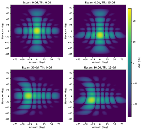
Figure 4: Composite phased-array antenna patterns of the next mobile-communications standard 5G as defined in ITU-R Rec. M.2101.

In pycraf several (simplified) antenna models are provided that implement various ITU-R recommendations, which shall be used for spectrum management studies. As an example, the fairly complex 5G composite antenna patterns can be obtained in the following manner:

Listing 5: 5G composite antenna patterns.

⬇

1import numpy as np

2import astropy.units as u

3import pycraf.conversions as cnv

4import pycraf.antenna as ant

5

6azims = np.arange(-180, 180) * u.deg

7elevs = np.arange(-90, 90) * u.deg

8

9# antenna parameters according to

10# ITU-R Rec. M.2101

11G_Emax = 5 * cnv.dB

12A_m, SLA_nu = (30, 30) * cnv.dimless

13azim_3db, elev_3db = (65, 65) * u.deg

14d_H, d_V = (0.5, 0.5) * cnv.dimless

15N_H, N_V = 8, 8

16

17azim_i, elev_j = (0, 0) * u.deg

18

19gains = ant.imt2020_composite_pattern(

20 azims[np.newaxis],

21 elevs[:, np.newaxis],

22 azim_i, elev_j,

23 G_Emax,

24 A_m, SLA_nu,

25 azim_3db, elev_3db,

26 d_H, d_V,

27 N_H, N_V,

28 )

where the azim_i and elev_j angles define the pointing of the formed beam in the antenna frame coordinates (azimuth and elevation). In Fig. 4 examples are shown for four different beam directions: $(0^{\circ},0^{\circ})$, $(30^{\circ},0^{\circ})$, $(0^{\circ},15^{\circ})$, and $(30^{\circ},15^{\circ})$.

2.5 Atmospheric attenuation

Once the propagation path exceeds a certain length, e.g., for communication links to satellites or for radio-astronomical observation of extra-terrestrial sources, the attenuation by the gases in the atmosphere of the Earth becomes important, especially at higher frequencies. Again, there exists a ITU-R recommendation, P.676, which was implemented in the atm sub-package. It can be used to predict the attenuation as a function of frequency, path geometry, and atmospheric parameters. The two molecules that play a major role are oxygen (so-called dry component) and water (wet component), both introducing spectral-line emission and absorption. Furthermore, oxygen also produces the continuous non-resonant Debye-spectrum (below 10 GHz). At frequencies above 100 GHz continuous attenuation by nitrogen starts to play a role as well.

The calculation of atmospheric attenuation is performed via a ray-tracing approach. Let us assume a radio signal enters Earth’s atmosphere and travels to a receiving station close to the ground. First, the atmosphere is divided into layers (several hundreds or more) and for each of these the attenuation of the incident signal is calculated, such that the signal, which leaves a layer is somewhat weaker than the signal that entered a layer. At the same time, the layer itself emits radio waves having the aforementioned spectral properties. Each layer has different physical properties, such as temperature, pressure, water content, and refractivity. These “height profiles” have to be known to calculate the specific attenuation per layer. For ITU-R related studies, it is widely accepted to work with mean profiles, which were averaged over a year. The “standard profile” is provided in ITU-R Rec. P.835 along with five more specialised profiles, associated with the geographic latitude and season (“high-latitude summer/winter”, “mid-latitude summer/winter”, and “low latitude”). For example:

Listing 6: Atmospheric attenuation.

⬇

1import numpy as np

2import astropy.units as u

3import pycraf.conversions as cnv

4from pycraf import atm

5

6# define height grid

7height_grid = np.arange(0, 85, 0.1) * u.km

8

9# query profile_standard function

10(

11 temperatures,

12 pressures,

13 rho_water,

14 pressures_water,

15 ref_indices,

16 humidities_water,

17 humidities_ice

18 ) = atm.profile_standard(height_grid)

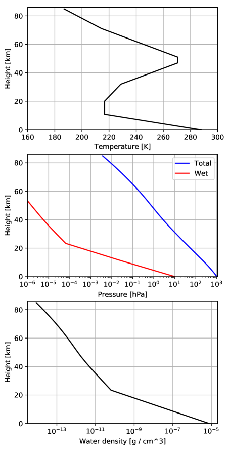
Figure 5: Standard atmospheric height profiles (temperature, pressure, and water density) according to ITU-R Rec. P.835.

The resulting profiles are displayed in Fig. 5. ITU-R Rec. P.676 contains tables with the resonance lines of oxygen and water, necessary to calculate the specific attenuation for one layer (or propagation paths close to the ground, which stay in a single layer). The function atten_specific_annex1 can be used for that:

⬇

28freqs = np.arange(1, 1000) * u.GHz

29p_total = 1013 * u.hPa

30temperature = 290 * u.K

31rho_water = 7.5 * u.g / u.m ** 3

32

33# need dry and wet pressure separately:

34p_wet = atm.pressure_water_from_rho_water(

35 temperature, rho_water

36 )

37p_dry = p_total - p_wet

38

39print(’O2 pressure: {:.2f}’.format(p_dry))

40print(’H2O vapor partial pressure: ’

41 ’{:.2f}’.format(p_wet))

42# Oxygen pressure: 1002.96 hPa

43# Water vapor partial pressure: 10.04 hPa

44

45a_dry, a_wet = atm.atten_specific_annex1(

46 freqs, p_dry, p_wet, temperature

47 )

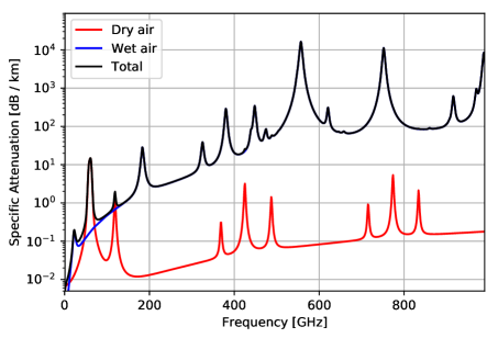
Figure 6: Specific attenuation for a layer with a total pressure of 1013 hPa, a temperature of 290 K, and a specific water density of $7.5\leavevmode\nobreak\ \mathrm{g\,cm}^{-3}$ according to ITU-R Rec. P.676.

The resulting spectrum is shown in Fig. 6. Calculating such spectra for each layer allows us to perform the ray-tracing for a slant path through the full atmosphere (with the function atten_slant_annex1):

⬇

18elevation = 15 * u.deg

19station_altitude = 300 * u.m

20freqs = np.arange(1, 100, 0.1) * u.GHz

21

22(

23 total_atten, refraction, tebb

24 ) = atm.atten_slant_annex1(

25 freqs, elevation,

26 station_altitude,

27 atm.profile_highlat_winter

28 )

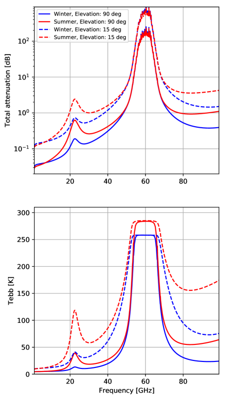
Figure 7: Atmospheric attenuation of a slant path for Summer/Winter high-latitude standard profiles according to ITU-R Rec. P.676. The lower panel shows the equivalent-black-body temperature of the full atmosphere.

In Fig. 7 the total atmospheric attenuation of a slant path for Summer/Winter high-latitude standard profiles is presented, along the so-called equivalent-black-body temperature, $T_{\mathrm{ebb}}$, of the full atmosphere with major contributions by the atmospheric emission itself.

2.6 Satellite two-line elements

For studies involving a satellite or a satellite network it is often necessary to determine their position relative to an Earth station. Satellite orbits vary slowly in time as a consequence of the gravitational influence of planetary system bodies, most importantly the Moon, the Sun, and Jupiter. Furthermore, the orbits are subject to drag forces induced by the outer layers of the atmosphere, especially, in the case of low-earth orbit (LEO) satellites. Satellites are therefore constantly monitored by stations on Earth to update their orbital parameters. These are provided in a standardized format, the so-called two-line element (TLE) sets, which are usually updated once per day and can be retrieved from the Space Track or CelesTrak websites. As an example, the TLE of the International Space Station (ISS) for September, 20, 2008 looks like this:

⬇

ISS (ZARYA)

1 25544U 98067A 08264.51782528 -.00002182 00000-0 -11606-4 0 2927

2 25544 51.6416 247.4627 0006703 130.5360 325.0288 15.72125391563537

The meaning of the entries is described e.g. on Wikipedia. The fields 7 and 8 (line 1, columns 19–20 and 21-32), i.e., 08 and 264.51782528 encode the epoch (year and day of year) at which the other orbital parameters are valid. From this point in time, one can then propagate the orbit.

To account for the aforementioned distortions of orbits, the calculations behind the propagation algorithm are rather complex and pycraf internally uses the Python package sgp4 for this. Provided with a TLE string, sgp4 can calculate the position of the satellite in the Geocentric reference frame for any point in time. However, if the time difference to the TLE epoch is significantly larger than a day, the result may be completely wrong.

For compatibility studies one usually needs the satellite position in the antenna reference frame of the ground station. Therefore, the satellite sub-package of pycraf, which is otherwise just a thin wrapper around sgp4, adds some routines for this coordinate conversion. One only needs to specify the coordinates of the observatory and the desired time:

Listing 7: Satellite TLEs.

⬇

1from astropy import coordinates, time

2from pycraf import satellite as sat

3

4tle_string = ’’’ISS (ZARYA)

51 25544U 98067A 08264.51782528 ...

62 25544 51.6416 247.4627 0006703...’’’

7

8# define observer location

9loc = coordinates.EarthLocation(

10 6.88375, 50.525, 366.

11 )

12

13# create a SatelliteObserver instance

14sat_obs = sat.SatelliteObserver(loc)

15

16obstime = time.Time(

17 ’2008-09-20T20:00:00.000000’,

18 format=’isot’, scale=’utc’

19 )

20

21az, el, dist = sat_obs.azel_from_sat(

22 tle_string, obstime

23 )

24print(’Azimuth : {:6.1f}’.format(az))

25print(’Elevation: {:6.1f}’.format(el))

26print(’Distance : {:6.1f}’.format(dist))

27# Azimuth : 80.1 deg

28# Elevation: 11.1 deg

29# Distance : 1257.7 km

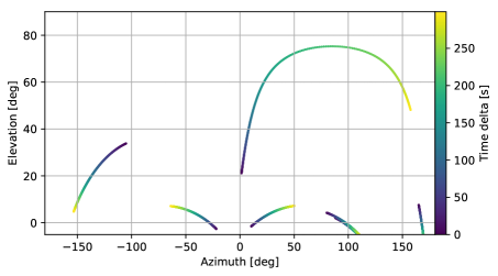
Figure 8: Position of visible IRIDIUM network satellites in the topocentric reference frame for an observer at the Effelsberg observatory. Displayed are the azimuth and elevation of the satellites for five minutes starting from January, 4, 2018, 21:45 (UTC).

As another example, Fig. 8 shows the position of the IRIDIUM network satellites, as seen from an observer at the Effelsberg observatory. IRIDIUM satellites are LEOs and move fast over the visible sky. To visualize this, the azimuth and elevation of the satellites were computed for a time range of five minutes.

3 Compatibility of a 5G cell phone network and RAS

With the pycraf package introduced in Section 2.1 it is very easy to do simple compatibility studies. Especially, for a point-to-point analysis, there is not much more to it than the determination of the emitted power and the path loss and finally the comparison of the received power with the compatibility threshold level. These steps could easily be put into a stand-alone software package, perhaps with a graphical user interface. A need for additional functionality may however arise sometimes, or one may be faced with more complex scenarios right from the beginning. Therefore, pycraf was designed as a programming library. Although this makes the simplest projects slightly more complicated (because one always need to write some Python code), it is well-suited to deal with more challenging studies. One of these more complicated cases is discussed in this section.

3.1 Context

The mobile telecommunication industry wants to utilize more bandwidth for their next-generation mobile communications standard, which is called 5G. At the last world radio communications conference (WRC), an agenda item (AI 1.13) was proposed for the next WRC in 2019. It is entitled “Work plan and proposed liaison to Task Group 5/1 on spectrum needs for the terrestrial component of IMT in the frequency range between 24.25 GHz and 86 GHz”. Although there is currently some tendency among vendors and administrations to favour the lower part of the frequency range mentioned in the agenda item (the 24.25–27.5 GHz sub-band) we are required to study all possible sub-bands without a predetermined conclusion for AI 1.13.

The Committee on Radio Astronomy Frequencies (CRAF) – an expert committee of European radio astronomers involved in spectrum management – is submitting input documents with compatibility studies to various regional and global working groups (ITU-R TG 5/1, ECC PT 1). These studies attempt to determine the compatibility of the next-generation 5G equipment with radio-astronomical observations. Depending on the designated 5G band, protected RAS bands would in some cases be located in the out-of-band (OOB) or spurious domain with respect to the IMT carrier frequency, in other cases we may face the in-band sharing scenario, where both, Tx and Rx, frequency ranges overlap. The latter case usually demands larger separation distances between interfering stations (the IMT equipment) and the victim station (the radio telescope) to ensure that radio-astronomical observations do not suffer interference. Because of the additional attenuation of the emitted power a compatibility is more easily obtained in the OOB or spurious cases.

Here, we describe how the compatibility calculations for one of these studies were made, focussing on the 24.25–27.5 GHz frequency band. RAS has a primary allocation for 23.6–24 GHz, hence, this is an example for a OOB-domain scenario. For compatibility studies on the ITU level, one often analyses the “generic” case, where no terrain height (above the Earth ellipsoid) is assumed, so that the results do not depend on the terrain details of specific sites. Of course, RAS stations in mountainous regions may have some level of natural shield from surrounding hill tops, so that generic-study results are only indicative. Still, many RAS stations are located in regions with relatively flat terrain, e.g., the Westerbork Synthesis Radio telescope in the Netherlands.

We emphasize that the results presented here sensitively depend on the chosen transmitter properties and deployment densities. The assumptions and values, which are used in the following, are preliminary, as some of relevant (ITU-R) recommendations and guidelines are not yet finalized. Therefore, one should be careful with drawing conclusions from our study.

3.2 Setup I: Transmitter and receiver properties

5G networks will likely be “classic” mobile networks, consisting of base stations (BS) and user equipment (UE), although alternatives such as mesh-network based topologies seem also viable. Both, BS and UE feature phased-array antenna patterns, as described in Section 2.4. The transmitter properties (to be used for compatibility calculations) are summarized in ITU-R Doc. TG 5/1-36 (Attachment 2). For BS, $8\times 8$ individual antenna elements, each having a power output of 10 dBm per carrier (before Ohmic losses), are foreseen. UE will use smaller arrays, of $4\times 4$ elements, but with the same power levels. For the spurious domain, a spectrum block edge mask of $-$38 dBc per carrier bandwidth (200 MHz) for BS and $-$32 dBc/carrier for UE is in place, such that the spectral power density within the RAS band is $-$13 dBm/MHz in both cases. For UE an additional so-called body loss of 4 dB has to be accounted for, because in many situations a person holding the user device (e.g., a smart phone) will provide additional shielding. Integrating the spectral power over the RAS band yields a total of 13 dBm.

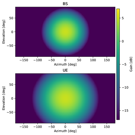
Figure 9: Single-element antenna patterns of the next mobile-communications standard 5G as defined in ITU-R Rec. M.2101.

ITU-R Doc. TG 5/1-36 (Attachment 2) makes a distinction for different zone types, urban, suburban and suburban open-space regions with different number densities and antenna heights. BS antenna heights will be 15 m for suburban open-space zones and 6 m for the rest, while UE is always at 1.5 m height. Even though the 5G phased array antennas allow dynamic beam forming, ITU-R Rec. M.2101 advises to use the single-element patterns for studies in the spurious domain. We follow this advice here, although there are diverging opinions about it as some consider it unlikely that the signal phasing should be completely inefficient close to the carrier frequency. Fig. 9 shows the resulting antenna gain patterns for BS and UE, respectively. The composite antenna patterns will still be required (see Section 3.6), because they influence the link budget (or coupling loss) between BS and UE, which in turn determines the level of power control in the user devices – UE can increase or decrease the transmitted power based on the coupling loss for more efficient battery use.

On the receiver side, an isotropic antenna (0 dBi) is usually assumed for these kinds of studies, with a height of 50 m above ground, which would be typical for a 100-m class radio telescope. ITU-R Rec. RA.769 permits an interference power level of $-$165 dBm (in continuum mode). Therefore, the minimal coupling loss (MCL), i.e., the attenuation induced by the path propagation loss plus the gain or attenuation due to the Tx antenna gain, must be at least 178 dB. The MCL ultimately determines the minimal distance (also called separation distance) that a device must have from the Rx to avoid problems with RAS observations.

3.3 Path propagation loss

With the functionality contained in pycraf, it is very easy to determine the path loss as a function of distance between Tx and Rx. Here, a distinction is to be made between the sub-/urban and suburban open-space areas, because the antenna height plays a role for the propagation. The default clutter model of ITU-R Rec. P.452 is not be applied in studies related to agenda item AI 1.13, instead the use of the model provided in ITU-R Rec. P.2108 is mandatory. It depends only on frequency, distance, and a quantity called location percentage, $p_{\mathrm{L}}$, which is the percentage of all emitters producing the lowest clutter loss. For example, if $p_{\mathrm{L}}=2\%$, the returned value, $L_{\mathrm{clutter}}$, indicates that for 2% of all devices the actual clutter loss will fall short of $L_{\mathrm{clutter}}$. In other words, P.2108 provides the cumulative distribution function for the clutter. We also note that the distance dependence in ITU-R Rec. P.2108 is only relevant for very small values below $\sim$2 km.

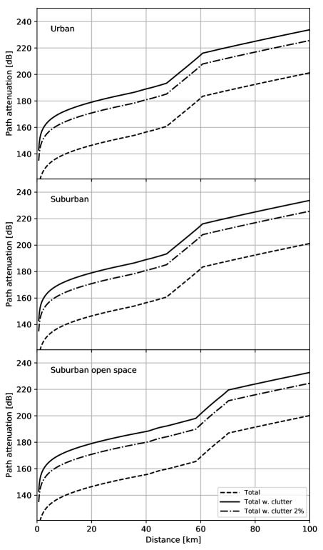
Figure 10: Path propagation loss for BS at 24 GHz according to ITU-R Rec. P.452 (dashed line). The black solid line includes the median clutter loss predicted by ITU-R Rec. P.2108, the dash-dotted line was computed for a location percentage of $p_{\mathrm{L}}=2\%$ (see text).

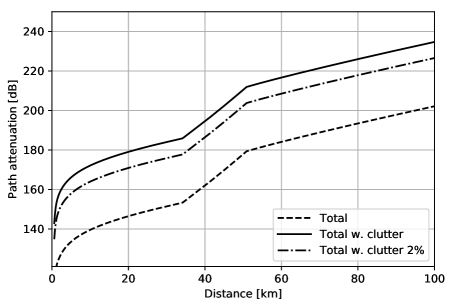
Figure 11: As Fig. 10 for UE.

In Figs. 10 and 11 the resulting path propagation loss for BS and UE is displayed. The rapid increase of the path loss between about 35 and 50 km is caused by the geometry of the path. There, the line-of-sight path (small distances) turns into a trans-horizon path, meaning that diffraction kicks in.

3.4 Single-interferer scenario

The single-interferer scenario is an extreme case, where only one IMT device is considered having maximally possible antenna gain (i.e., the antenna shall be directed towards the RAS station) and very low $p_{\mathrm{L}}$ (which means the clutter loss will be unusually small). In reality, such a situation will rarely occur, but it is still valuable to study this case, because it already gives a rough indication about the magnitude of the necessary separation distances. Very often, the single-interferer separation distances define a zone, where operation of the interfering service will be critical.

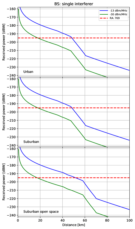
Figure 12: Received power levels of a BS for the worst-case single interferer scenario. Two different spurious-domain Tx power levels were assumed. The red dashed line is the RA.769 threshold, which should not be exceeded.

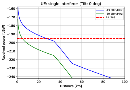
Figure 13: As Fig. 12 for UE.

Figures 12 and 13 contain the resulting power levels received from a single BS or UE with the isotropic RAS antenna. The RA.769 threshold is marked by a dashed red line. The crossing point of the curves with the threshold defines the necessary separation distance. We note that for IMT networks of the previous generations, a spurious power level of $-30$ dBm/MHz was in place in Europe. To allow for comparison, the figures also contain the results for this lower level.

3.5 Setup II: Deployment of 5G devices

More important than the single-interferer analysis is the calculation of the received aggregated power levels, which stem from the full IMT network as the sum of powers from each individual device. Here one aims to use a realistic scenario for the deployment of the IMT equipment to the best of one’s knowledge. This not only involves modelling how the BS and UE are distributed in a given area, but one must also account for the quasi-random orientations that the BS and especially the user devices may have. The latter can e.g. be freely rotated with respect to the BS.

Both, BS and UE will use phased-array technology to form beams into the direction of the associated communication partner. Relatively high gains can be achieved this way, even with the small antenna apertures. BS, which are associated to several user devices simultaneously, use the time-division duplex (TDD) method to serve the UE. In each time slot, the phased-array weights are updated to form a beam to the currently active device. The BS antenna frames themselves are fixed, in contrast to the user devices, where the system needs to form the beam depending on the location relative to the BS and its current rotation state. The beam forming also has an impact on the power that is transmitted into the direction of the RAS station, because the beam direction will significantly change the side-lobe pattern of the antennas (compare Fig. 4).

Due to the TDD, each user device is only active during 20% of the time. For BS the TDD factor is set to 80%. Furthermore, in reality the network as a whole never runs at full capacity. For scenarios such as the one analysed here, ITU-R Doc. TG 5/1-36 (Attachment 2) recommends to work with a network loading factor of 20%.

In ITU-R Doc. TG 5/1-36 (Attachment 2) typical number densities are provided, which shall be used for generic compatibility studies involving large areas. The densities differ for BS and UE, but also for the various zone types. The parametrization is done in terms of the percentage of the considered area that has housing, $R_{\mathrm{b}}=5\%$, and the fraction within this area that is expected to have 5G installations, $R_{\mathrm{a}}$. For urban zones, $R_{\mathrm{a}}^{\mathrm{urb}}=7\%$, while in suburban areas $R_{\mathrm{a}}^{\mathrm{sub}}=3\%$. Within the so-defined regions, 30 BS (100 UE) for urban and 10 BS (30 UE) for suburban zones are expected to be installed on average. For suburban open-space zones, the numbers are 1 BS (30 UE).

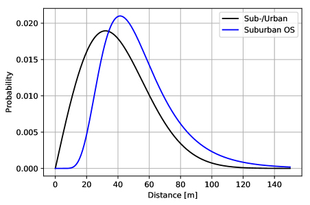
Figure 14: Distribution for UE as a function of distance from associated BS.

The final ingredient is the location of the UE relative to the associated BS. ITU-R Doc. TG 5/1-92 (Annex 1) defines distribution functions for the distance (Rayleigh for urban/suburban; Log-Normal for suburban open-space) and azimuthal position (Normal, $\mathcal{N}(0^{\circ},30^{\circ})$) relative to the antenna normal vector. The two distance distributions are displayed in Fig. 14. It should be noted that each BS features only one sector antenna, in accordance to ITU-R Doc. TG 5/1-36 (Attachment 2).

In ITU-R Rec. M.2101 several possible deployment topologies are discussed, e.g., hexagonal or Manhattan-style grid layouts. In the particular case that is analysed here, the network topology can be neglected because one needs to average over a very large region, such that the aggregated power at the RAS station will be dominated by the (constant) deployment densities defined in ITU-R Doc. TG 5/1-36 (Attachment 2).

3.6 Aggregated power levels

We use a Monte-Carlo sampling approach to calculate the aggregated powers from the IMT network. This means that random values for BS and UE positions and rotations are generated from the distribution functions discussed in Section 3.5. This process is repeated many times and for each realization the total power received at the RAS station is calculated. From the ensemble of received powers (one value per trial run), one can then study distribution properties such as the median or average power level, but also the uncertainties (spread about the median).

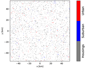
Figure 15: Zone types (urban and suburban) randomly assigned to grid cells in the simulated box following a uniform distribution function.

The first step in our aggregation analysis is to generate a map containing zone types. A sufficiently large box of size $400\leavevmode\nobreak\ \mathrm{km}\times 400\leavevmode\nobreak\ \mathrm{km}$, with grid cells of size $0.5\leavevmode\nobreak\ \mathrm{km}\times 0.5\leavevmode\nobreak\ \mathrm{km}$ is created. For each cell, a random number from a uniform distribution, $\mathcal{U}(0,1)$, is drawn. Cells with values between $1-(R_{\mathrm{a}}^{\mathrm{urb}}+R_{\mathrm{a}}^{\mathrm{sub}})R_{\mathrm{b}}$ and $1-R_{\mathrm{a}}^{\mathrm{urb}}R_{\mathrm{b}}$ are classified as suburban, while values larger than $1-R_{\mathrm{a}}^{\mathrm{urb}}R_{\mathrm{b}}$ define urban areas. (Regions with housings are defined by values exceeding $1-R_{\mathrm{b}}$.) Figure 15 shows a zoom-in to the central part of the simulated box, with the random zone types assigned to it.

One could argue that such uniform-density deployment is not very realistic. Therefore, as an alternative we develop an algorithm that produces zones, which better resemble a real-world distribution of urban and suburban areas (inspired by the situation around the Effelsberg observatory). For this, some kind of clustering has to be introduced. One possibility to achieve that, is by smoothing the random numbers with one or more Gaussian filter kernels before assigning the zone types. The smoothing introduces a correlation between neighbouring pixels. The larger the smoothing radius, the stronger the clustering of zone types will be. We find that a combination of three different kernels with scales $\sigma_{\mathrm{k}}=2$, 5, and 15 km and relative amplitudes of 30%, 30%, and 40% can produce a zone-type map, which seems to be quite realistic; see Fig. 16.

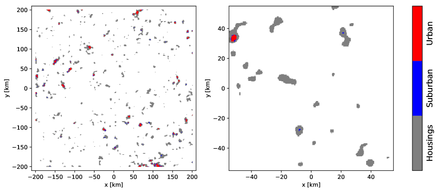
Figure 16: Zone types (urban and suburban) randomly assigned to grid cells in the simulated box based on the clustering algorithm described in the text. The right panel shows the full box, the right panel a zoom-in to the central area.

Into the grid cells, BS are now sampled according to the zone types and given number densities. For each BS, a random azimuthal orientation of the antenna frame is assigned, and the tilting angle in elevation is considered. UE has to be handled differently, because several user devices can be associated to each BS, and the locations of the UE must be in the respective forward cone of the BS. Therefore, for each BS, user devices are sampled into the forward cone, until the total number of UE fits the desired global number density (per zone). UE can be freely rotated, with the only restriction, that the angular distance between antenna normal vector and direction to the associated BS shall not exceed $60^{\circ}$; see ITU-R Doc. TG 5/1-92 (Annex 1). Such a general rotation can for example be constructed from three Euler-angle rotations. Initially, the UE antenna normal shall point to the BS. We first rotate randomly about the UE–BS vector, then about the axis that is perpendicular to the UE–BS vector, is parallel to the $x$–$y$ plane (the ground) and includes the UE position. Finally, another rotation about the UE–BS vector is applied. The first and last rotation angles are drawn uniformly from the interval $\left[-180^{\circ},180^{\circ}\right]$, while the second rotation has random angles from $\left[-60^{\circ},60^{\circ}\right]$. The resulting rotation has the desired properties.

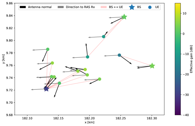
Figure 17: Effective antenna gains into the direction of the RAS Rx. The BS and UE are colourized according to the gain. Red solid lines show BS–UE vectors. Black arrows indicate the antenna frame normal vectors, while gray arrows point to the RAS Rx.

The next step is to calculate the effective antenna gains of each 5G device towards the RAS station. Since the positions and orientations of all devices are known, one can easily determine the azimuth and elevation of the UE–BS vectors, as well as of the direction to the RAS Rx, in the (rotated) antenna frames. Strictly speaking, if the single-element antenna patterns are used, the UE–BS vectors are irrelevant. However, they will be needed for the power control algorithm, which is discussed below. Using the antenna gain formula provided in ITU-R Rec. M.2101 (implemented in pycraf.antenna), the effective gains follow directly. For BS, there is not a single resulting gain value, but several – one for each user device in the forward cone. Therefore, the average value is calculated and applied in the following. Figure 17 visualizes the geometry and the determined effective gains for a small sub-region that includes three BS and their associated UE. The red lines mark which user device belongs to which BS. The black arrows are the antenna normal vectors (projected into the $x$–$y$ plane, i.e., shorter arrows have larger $z$ components), while grey arrows point to the RAS station. The more the black and grey arrows are aligned, the higher the effective gain. If the composite patterns would be used, the arrows additionally had to be aligned with the red BS–UE vectors to produce highest effective gain. However, the beam forming makes the latter alignment less important. Only if the beam direction has large angular separation from the antenna normal, the achievable gain towards the beam direction drops significantly. However, the specific side-lobe patterns play an important role in the composite-antenna case.

The path propagation loss to the RAS Rx is then computed for each 5G device, as discussed in Section 3.3, such that all necessary quantities to determine the total power level are now known. There is one last aspect, which makes the calculation slightly more complex: the power control algorithm mentioned in Section 3.2. For this, the link budget between BS and UE has to be determined (according to 3GPP TR 38.901, UMi – Street Canyon scenario). The details are beyond the scope of this paper. If the coupling loss between BS and UE is low, a user device may decrease the transmitter power to save battery power (according to a formula provided in ITU-R Rec. M.2101). The power control leads to a somewhat lower aggregated UE power, but since BS have a much larger impact on the total power (and are not subject to power control), the change is insignificant.

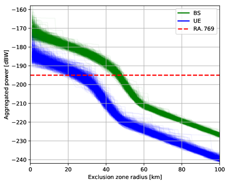
Figure 18: Cumulative aggregated power as a function of exclusion zone radius, $r_{i}$ for uniform distribution of housings. The results of all 1000 Monte-Carlo trials are shown.

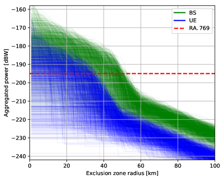
Figure 19: As Fig. 18, but for the clustered distribution of housings.

The aggregated powers received at the RAS station exceed the ITU-R Rec. RA.769 thresholds in every single Monte-Carlo run. This is not unusual because there is always a high chance that some devices get placed too close to the RAS Rx. To find out, how big an exclusion zone (i.e., the lower limit of separation distances to each device) would need to be, we show cumulative plots of the aggregated powers in Figs. 18 and 19. For increasing radii, $r_{i}$, devices within a sphere with this radius are left out from the aggregation. The larger $r_{i}$, the lower becomes the received power, as only more distant devices contribute. In total, one thousand runs were carried out. For each of these realizations, Fig. 18 contains the cumulative distribution for both, BS and UE, in the uniform-density scenario. Figure 19 shows the results for the clustered-density approach, revealing much higher scatter.

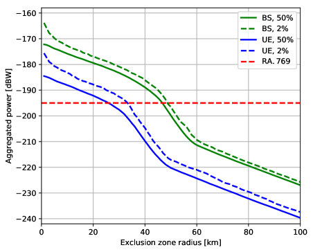
Figure 20: Ensemble percentiles (50% and 98%) for the distribution of aggregated powers shown in Fig. 18.

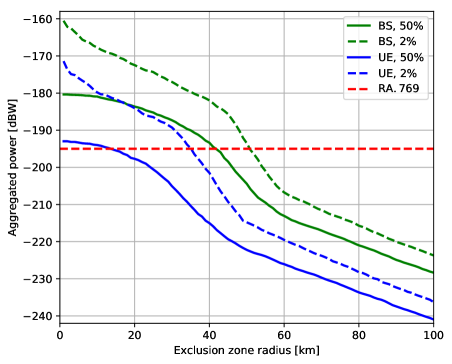
Figure 21: As Fig. 20, but for the clustered distribution of housings.

In order to determine a single value for the necessary exclusion zone radius, we compute distribution percentiles at 50% (the median) and 98% (the top 2% level); see Figs. 20 and 21. As can be seen, BS produce on average more than 10 dB higher aggregation levels than UE. Furthermore, there is a steep regime between 30 km and 60 km, where the power level drops quickly. This behaviour can be attributed to the path propagation loss, which shows a similar kink (compare Figs. 10 and 11). Hence, the transmitted power levels could be increased substantially, without the exclusion zone size having to grow quickly (unless one would not want to accept separation distances of $\sim$60 km in the first place).

The pycraf package proves to be a valuable and versatile tool to assist spectrum managers with accomplishing compatibility studies. In simpler cases, this only needs a few lines of Python code, but being a programming library, pycraf is also useful for very complex analyses, e.g., full Monte Carlo simulations of mobile communication networks.

Such a case, a compatibility study involving next-generation 5G at 24 GHz and a RAS telescope, was presented in detail. In the generic case (flat-earth, i.e., zero terrain heights) the aggregated power levels produced at the radio-astronomical receiver would exceed the maximally permitted thresholds defined in ITU-R Rec. RA.769 unless an exclusion zone with a radius of few tens of kilometres would be established.

The pycraf library is made available on the Python package distribution server PyPI (Python Package Index, https://pypi.python.org/pypi/pycraf). It is open source software licensed (GNU General Public License v3.0). The source code is hosted on the GitHub platform (https://github.com/bwinkel/pycraf) and is also available on Zenodo (https://doi.org/10.5281/zenodo.1244192). Contributions are welcome.

The authors declare that they have no conflict of interest.