Equilibrium configuration of self-gravitating charged dust clouds: Particle approach

Abstract

A three dimensional Molecular Dynamics (MD) simulation is carried out to explore the equilibrium configurations of charged dust particles. These equilibrium configuration are of astrophysical significance for the conditions of molecular clouds and the interstellar medium. The interaction among the dust grains is modeled by Yukawa repulsion and gravitational attraction. The spherically symmetric equilibria are constructed which are characterized characterized by three parameters: (i) the number of particles in the cloud, (ii) $\Gamma_{g}$ (defined in the text) where $\Gamma_{g}^{-1}$ is the short range cutoff of the interparticle potential, and (iii) the temperature of the grains. The effects of these parameters on dust cloud are investigated using radial density profile. The problem of equilibrium is also formulated in the mean field limit where total dust pressure which is the sum of kinetic pressure and electrostatic pressure, balances the self-gravity. The mean field solutions agree well with the results of MD simulations. Astrophysical significance of the results is briefly discussed.

I Introduction

Dust is one of the main constituents of the universe and plays a central role in the formation of stars and planetsHarpaz (1993); Desch (2004); Hartmann (1983). A variety of astrophysical systems such as interstellar clouds, solar system, planetary rings, cometary tails, Earth’s environment etc. contain micron to sub-micron sized dust particles in different amounts Verheest (2000). However, in the presence of ambient plasma and radiative environments, these particles are acted upon by the electron-ion currents, photons and energetic particles. As a result, the dust grains acquire a non-negligible electric charge (which is usually negative) and start interacting with each other, as well as with ions and electrons via long-range electric fields giving rise to collective behavior. This leads to the formation of special medium called the “dusty plasma”.

The macroscopic particles in dusty plasmas interact not only via electric field but also via gravitation field which is also a long ranged force. Which of the forces dominates, is determined by the ratio of average gravitational potential energy to average electrostatic (ES) potential energy. If $m_{d}$, $Q_{d}$ be the mass, charge of a dust grain and $n_{d}$ be the number density then the gravitational potential $\psi$ is given by Poisson’s Equation, $\nabla^{2}\psi=4\pi Gm_{d}n_{d}$ which scales as $\psi\approx 4\pi Gm_{d}n_{d}L^{2}$, therefore, average gravitational energy of a dust grain may be given as $m_{d}\psi\approx 4\pi Gm_{d}^{2}n_{d}L^{2},$ where $G$ is the universal gravitational constant and $L$ is the typical length scale over which dust is distributed. Similarly, the ES potential $\phi$ for dust is given as $\nabla^{2}\phi=-Q_{d}n_{d}/\epsilon_{0}$, thus, $\phi$ scales as $\phi\approx-Q_{d}n_{d}L^{2}/\epsilon_{0}$ and average ES potential energy scales as $Q_{d}\phi\approx Q_{d}^{2}n_{d}L^{2}/\epsilon_{0}$ and the ratio of two energies comes out to $Gm_{d}^{2}/(Q_{d}^{2}/4\pi\epsilon_{0})$. For typical plasmas of size of order of microns and charge of the order of $10^{3}\;e$, the ratio comes out to be $\approx\mathcal{O}(10^{-17})$. However, in dusty plasmas, the electric field is screened substantially by the presence of the background electrons and ions. The estimate of ES potential, in such case, should be made using the quasi-neutrality condition $Q_{d}n_{d}=e(n_{i}-n_{e})$. Taking the electron and ion response as Boltzmannian i.e. $n_{\alpha}=n_{0}\exp(q_{\alpha}\phi/k_{B}T_{\alpha})$ where $\alpha=$(electron, ion), $T_{\alpha}$ is the temperature of spices $\alpha$ and $n_{0}$ is the mean plasma density in the region where $\phi=0$, the ES energy scales as $Q_{d}\phi\approx Q_{d}^{2}n_{d}\lambda_{D}^{2}/\epsilon_{0}$, where $\lambda_{D}=\left({e^{2}n_{0}(T_{e}+T_{i})}/{\epsilon_{0}k_{B}T_{e}T_{i}}\right)^{-1/2}$ is the Debye screening length. Therefore, the ratio of gravitational energy to electrostatic energy in the presence of background plasma becomes $Gm_{d}^{2}L^{2}/(Q_{d}^{2}\lambda_{D}^{2}/4\pi\epsilon_{0})$. Since, the typical length scale of dust cloud, $L\gg\lambda_{D}$ therefore, the ratio $Gm_{d}^{2}L^{2}/(Q_{d}^{2}\lambda_{D}^{2}/4\pi\epsilon_{0})$ could be $\approx\mathcal{O}(1)$. Therefore, for the micron sized particles the forces due to screened ES fields and gravitational force are comparable on sufficiently long length scales $L$ which may be found in the astrophysical scenarios.

The Jeans instabilityJeans (1929) is the most fundamental instability in the self-gravitating systems which plays a crucial role in the formation of structures in the universe. Physically, whenever there is an imbalance between the self-gravitating force and the internal pressure of a gas, the Jeans instability appears. The threshold for the Jeans instability in self-gravitating neutral fluid is set by the hydrostatic pressure of the fluidChandrasekhar (1961). In case of dusty plasmas, the neutral mass density is replaced by the dust mass density and the neutral gas pressure is replaced by the sum of electron and ion pressure.

Therefore, the threshold for Jeans instability is set by the dust acoustic wavesRao et al. (1990) instead of the usual sound wavesShukla and Stenflo (2006a); Pandey et al. (1994); Avinash and Shukla (1994); Pandey et al. (1999); Pandey and Dwivedi (1996); Rao and Verheest (2000). Jeans instability in quantum dusty plasmas is studied by a number of authors Shukla and Stenflo (2006b); Masood et al. (2008); Salimullah et al. (2009); Ren et al. (2009) and the effect of physical processes like magnetic field, radiative cooling, polarization, electron-ion recombination and dust charge fluctuations etc. on Jeans frequency is reported in Refs. [Prajapati and Chhajlani, 2010; Jain and Sharma, 2016; Jain et al., 2017]. One major problem encountered frequently in dealing with the self-gravitating matter is the formation of legitimate equilibrium. On the astrophysical scales, the dust kinetic pressure is too weak to balance the self-gravity which suggests that the dust clouds are gravitationally unstable.

Recently, Avinash and Shukla have shown a new way of forming stable dust structures by balancing the force due to self-gravity of the dustAvinash and Shukla (2006); Avinash et al. (2006). In the case of dusty plasmas, the equilibrium configuration of dust cloud (embedded in a background plasmas) can be constructed by balancing the the forces due to screened ES field and gravitational forces which as pointed out earlier, are comparable on sufficiently longer length scales. The electrostatic repulsion among dust grains is equivalent to an “electrostatic pressure”Avinash (2006). If dust gains are distributed inhomogeneously within the plasma background, the electrostatic pressure, like the kinetic pressure, expels the dust from the regions of high dust density to the regions of low dust density. Avinash and Shukla have also shown the existence of a mass limit for the total mass supported by ES pressure against gravity Avinash and Shukla (2006). At low dust density the ES pressure $P_{ES}$ scales quadratically with number density $n_{d}$ ($P_{ES}\propto n_{d}^{\gamma}~{},\gamma=2$). At very high dust densities ES pressure becomes independent of number density due to charge reduction caused by mutual screening of the grainsAvinash et al. (2003); Barkan et al. (1994) and as a consequence $\gamma\rightarrow 0$. This change of $\gamma$ from two to zero implies that with increasing dust density, $P_{ES}$ is not able to cope with the gravitation resulting an upper mass limit ($M_{AS}$). The physics of this mass limit is very similar to Chandrasekhar’s mass limit for white dwarfs where adiabatic index for hydrostatic pressure changes from $5/3$ to $4/3$ due to relativistic effects. If the mass of dust cloud exceeds this upper mass ($M>M_{AS}$) the ES pressure is not strong enough to balance the gravity and the system will undergo symmetric collapse under self-gravity Avinash and Shukla (2006); Avinash et al. (2006); Avinash (2010a). Using the energy principle, the stability of these charge clouds is formulated and it is established that collapse responsible for $M>M_{AS}$ is due to stability of radial eigen mode Avinash (2007a, b).

We, in this communication, revisit the equilibrium problem using molecular dynamics (MD) simulations. The particles are subject to Yukawa repulsion as well as gravitation attraction force. At the equilibrium of these forces, a spherically symmetric cloud is formed. We also probe the dust density distribution of these clouds using radial density profile. The dependence of the equilibrium structure on the number of particles $N_{d}$, dimensionless parameters $\Gamma_{g}$ and temperature of the grains is examined using radial density profile. Unlike the previous models Avinash and Shukla (2006); Avinash et al. (2006); Avinash (2007a); Borah and Karmakar (2015) which are based on fluid description, our approach is based on particle description. One can go from particle description to fluid description via proper ensemble averaging, a process commonly known as “coarse graining”. We have, therefore, also formulated the problem of equilibrium in the mean field limit in terms of force balance coupled with equation of state. The mean field solution are are compared with the MD results and the the two solutions are found to agree well with each other.

The equilibrium structures are of considerable interest because of their astrophysically relevant length and mass scales. It is well known that the dust particles of micron and sub-micron size are an important component of interstellar cloudsTurner et al. (1989). This dust, which is typically silicate or polycyclic aromatic hydrocarbon, is the dominant cause of opacity and reddening of the spectral energy distribution of radiation from distant starsEvans (1993); Krugel (2002). The HI and HII regions are the part of interstellar molecular clouds where hydrogen is found to exist in abundance along with other gases like He, CO and the dust grains. In the HI region, which are relatively cooler with temperature $\sim 100$ K, hydrogen is found in the neutral state. The HII regions which are spread over the size ranging from 0.01 pc to 10 pc (1 pc $=3.08\times 10^{16}$ m), are the part of molecular clouds where star formation has recently taken place. The HII regions are relatively hotter with temperature ranging from $5000\--10000$ K and hydrogen is found in the ionized state in this region. The ionization takes place mainly due to the UV radiation of the nearby stats. In this conducting medium the macroscopic dust grains pick the negative charge from the medium$\--$ typically due to the attachment of negative electrons on the dust surface. The charge on the dust surface depends on the plasma conditions and its magnitude is about $10^{2}\--10^{4}~{}e$ , where $e$ is the electronic charge. The typical mass of a micron sized dust is about $10^{10}\--10^{13}$ times the mass of proton. The high resolution data from Herschel space observatoryAnderson et al. (2012) suggest that the dust is very cold in the HII region and the typical range of dust temperature varies from $\sim 12\--40$ K.

In this scenario, the interstellar dust first undergo gravitational instability. This instability saturates when the electrostatic pressure becomes equal to the gravitation force density which results in formation of a tenuous dust clouds which are stable. In the later section of this paper, we will show that for the physical parameter of HII region, the equilibrium structure formed in this process have approximately same order of size as the size of clumps of clouds observedBraun and Kanekar (2005); Smith et al. (2012) in the interstellar medium. The density profile explored in this paper not only gives the important information about the matter and charge distributions inside the clouds but may also provide an important insight about optical thickness of the small scale structures observed in the interstellar medium.

The paper is organized in the following manner. In Sec. II the details of the model used and the assumptions made in the model are described briefly. In Sec. III, we describe the details of the interaction potential, normalization used and the methodology used for MD simulations. The simulation results are given in Sec. IV. The mean field solutions are derived in Sec. V and validation of simulation results with mean field solution is provided in Sec. VI. The summary of the work is given in Sec. VII where we have also have discussed the astrophysical significance of the present.

II Model

Our model consist of a finite sized dust particles embedded in a much larger background of warm hydrogen plasma consisting of electrons and protons. Such a situation could occur in the HII region, where dust clouds have been observedFischer and Duerbeck (1998) in the background of hydrogen plasma.

In the interstellar medium dust grains exhibit a varying range of size, mass and charge. However, we make a simplifying assumption that all the dust grains have same size and therefore, equal mass. The electron and ion are much lighter than dust grains i.e. $m_{d}\gg m_{i},~{}m_{e}$ and plasma temperature $T_{e}\approx T_{i}=T\gg T_{d}$. The charge on the dust particle, unlike the intrinsic charge on electron and ions, depends on the local plasma environment. The important mechanism which are responsible for the charging of the dust grains in the interstellar medium are the thermal flux of electrons and ions and the flux of the photo-electrons Spitzer (1968); Wickramasinghe and Hoyle (1991). The estimate of the dust charge in such case, can be made using orbital motion limited theory Shukla and Mamun (2015). We, in our model, assume that the charge on all the dust particle due to various physical processes is equal with constant magnitude $Q_{d}$. It should be noted here that the dust size plays an important role in determining dust mass and dust charge. If $r_{d}$ is the radius the dust particle then the dust mass $m_{d}\propto r_{d}^{3}$ whereas dust charge $Q_{d}\propto r_{d}$. However, in our simulation once we assign the mass and charge of the dust particles then size has no direct role to play in the equilibrium formation. Therefore, in our simulation, we can safely consider the dust particle as point particle with mass $m_{d}$ and charge $Q_{d}$.

In our model, we assume that only the massive dust particles are affected by the gravity and their response in MD simulation is taken into account by using Newton’s law of gravitation. The background plasma is considered to be unaffected by the gravity. This situation is likely to occur in the HII region where $T_{e}=T_{i}=T\approx 5000$ K and plasma density, $n_{0}\approx 10^{7}~{}m^{-3}$. For these parameters, the gravitational potential energy of plasma is less than their thermal energy i.e., $GM_{c}m_{i}/R_{c}\ll k_{B}T$ (where $m_{i}$ is the ion mass, $M_{c}$ and $R_{c}$ are respectively the mass and radius of the dust cloud). Therefore, the gravitational collapse of the plasma background may be neglected and we may consider a thermalized, static plasma background governed by the Boltzmann relation for electrons and ions, i.e., $n_{e}=n_{0}\exp(e\phi/k_{B}T),~{}n_{i}=n_{0}\exp(͑-e\phi/k_{B}T)$. Here $\phi$ is the local plasma potential and $\phi=0$ at infinity where dust density is zero i.e., $n_{d}=0$ and $n_{e}=n_{i}=n_{0}$. This is a reasonable assumption for the interstellar cloudsSpitzer (1968); Wickramasinghe and Hoyle (1991). The electrostatic interaction among dust grains embedded in the background of statistically averaged neutralizing plasma background is given by the screened Coulomb (or Yukawa) potential.

In the presence of self-gravity, the dust-dust interaction becomes,

$$\Phi(r)=\frac{Q_{d}^{2}}{4\pi\epsilon_{0}}\frac{e^{-r/\lambda_{D}}}{r}-\frac{Gm_{d}^{2}}{r},$$ (1)

which is the sum of Yukawa and gravitational potential energy. Here, $r$ is the distance between two dust particles and $\lambda_{D}$ is the screening length defined earlier. It is well known that thermodynamics of gravitating systems has problems due to absence of short range and long ranged cutoffs in the inter-particle potential. However, in self gravitating dusty plasmas the short range cutoff is naturally provided by the electrostatic repulsion and the long range cutoff is defined by the typical length scale of dust dispersion. Hence, thermal equilibria of self gravitating dusty plasma exist at all temperatures.

III Simulation Details

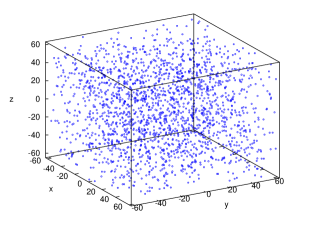
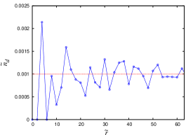
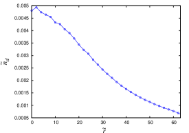
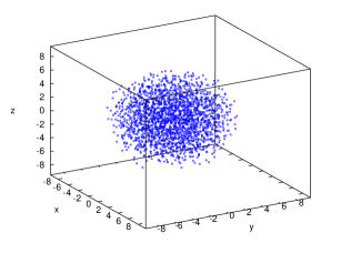
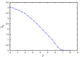
Figure 1: Different states of self-gravitating Yukawa particles is shown for $N_{d}=2000$. At the initial state particles are uniformly distributed in a cubical box with number density $\tilde{n}_{d}=0.001$ as shown in Fig.1 and corresponding radial density distribution is shown in Fig.1. Fig.1 refers to the equilibrium structure of the system where dust temperature $\tilde{T}_{d}=1.5$ and the corresponding density profile is shown in Fig.1. At lower temperature $\tilde{T}_{d}=0.5$ the equilibrium structure acquires the shape of sphere with a very dense core as shown in Fig.1. The averaged radial density of such dust cloud is shown in Fig.1.

III.1 Equations and Units

The Hamiltonian of the system is given by;

$$H=\sum_{i=1}^{N_{d}}\frac{p_{i}^{2}}{2m_{d}}+\frac{1}{2}\sum_{i=1}^{N_{d}}\sum_{j,j\neq i}^{N_{d}}\Phi(r_{ij})$$ (2)

where $r_{ij}=|\vec{r_{i}}-\vec{r_{j}}|$ and $p_{i}=|\vec{p}_{i}|$. We have assumed that all grains have equal charge $Q_{d}$ and mass $m_{d}$. The equation of motion are given by

$$\frac{d\vec{r}_{i}}{dt}=\frac{\vec{p}_{i}}{m_{d}},\\ \frac{d\vec{p}_{i}}{dt}=-\vec{\nabla}_{r_{i}}\left(\sum_{i=1}^{N_{d}}\sum_{j>i}^{N_{d}}\Phi(r_{ij})\right),$$ (3)

All the lengths are normalized by the background Debye length $\lambda_{D}$ and time is measured in units of $\omega_{0}^{-1}$ where $\omega_{0}=\left(Q_{d}^{2}/4\pi\epsilon_{0}m_{d}\lambda_{D}^{3}\right)^{1/2}$. Hence, $r\rightarrow\tilde{r}\lambda_{D}$ and $t\rightarrow\tilde{t}\omega_{0}^{-1}$, where $\tilde{r}$ and $\tilde{t}$ are dimensionless length and time respectively. Therefore, dimensionless equation of motion is

$$\frac{d\vec{\tilde{r}}_{i}}{d\tilde{t}}=\vec{\tilde{v}}_{i}\;,\>\frac{d\vec{\tilde{v}}_{i}}{d\tilde{t}}=\vec{\tilde{f}}_{i}$$ (4)

where

$$\vec{\tilde{f}}_{i}=\sum_{j,j\neq i}^{N_{d}}\left((1+\tilde{r}_{ij})\frac{e^{-\tilde{r}_{ij}}}{\tilde{r}_{ij}^{3}}-\frac{(4\pi\epsilon_{0}Gm_{d}^{2}/Q_{d}^{2})}{\tilde{r}_{ij}^{3}}\right)\vec{\tilde{r}}_{ij},$$ (5)

Temperature ($k_{B}T$) and energy is measured in units of $Q_{d}^{2}/4\pi\epsilon_{0}\lambda_{D}$ i.e. $\tilde{E}=E/(\frac{Q_{d}^{2}}{4\pi\epsilon_{0}\lambda_{D}})$ and $\tilde{T}_{d}=k_{B}T_{d}/(\frac{Q_{d}^{2}}{4\pi\epsilon_{0}\lambda_{D}})$. The dimensionless kinetic and potential energy per particles can be written as

$$\tilde{E}_{K} = \frac{1}{2N_{d}}\sum_{i=1}^{N_{d}}\tilde{v}_{i}^{2}~{},$$ (6)

$$\tilde{E}_{Pot} = \frac{1}{2N_{d}}\sum_{i}^{N_{d}}\sum_{j,j\neq i}^{N_{d}}\frac{(e^{-\tilde{r}_{ij}}-\Gamma_{g})}{\tilde{r}_{ij}}~{},$$ (7)

where $\Gamma_{g}$ is a dimensionless parameter defined as,

$$\Gamma_{g}=\frac{Gm_{d}^{2}}{(Q_{d}^{2}/4\pi\epsilon_{0})}.$$ (8)

In our simulations $\Gamma_{g}^{-1}$ defines the short range cutoff in inter-particle potential. In addition to this, $\Gamma_{g}$ also contains important information of various parameters of interest. As $\Gamma_{g}$ is directly proportional to $m_{d}^{2}/Q_{d}^{2}$, the effect of the dust mass, dust charge and dust size ($\Gamma_{g}\propto r_{d}^{4}$) can directly be seen from $\Gamma_{g}$.

Temperature is given by the mean kinetic energy per particle, which, in dimensionless units in 3D, turns out to be

$$\tilde{T}_{d}=\frac{1}{3N_{d}}\sum_{i=1}^{N_{d}}\tilde{v}_{i}^{2}=\frac{2}{3}E_{K}.$$

Normalized number density is given as,

$$\tilde{n}_{d}=n_{d}\lambda_{D}^{3}.$$

Dusty plasma equilibrium is defined in terms of two dimensionless parameters: $\kappa=a/\lambda_{D}$ and $\Gamma={Q_{d}^{2}}/{4\pi\epsilon_{0}aT_{d}}$ where $a$ is the mean inter-particle distance given by $a=\left(3/4\pi n_{d}\right)^{1/3}$. The coupling parameter $\Gamma^{*}=\Gamma\exp(-\kappa)$ which is the ratio of the mean inter-particle potential energy to the mean kinetic energy, is used as a measure of coupling strength in dusty plasmas. For $\Gamma^{*}\ll 1$, Yukawa system behaves like an ideal gas, $\Gamma^{*}\sim 1$ corresponds to an interacting fluid whereas $\Gamma^{*}\gg 1$ refers to a condensed solid state. The dimensional parameters $\kappa$ and $\Gamma$ can be related to normalized dust density and temperature as;

$$\kappa=\left(\frac{3}{4\pi\tilde{n}_{d}}\right)^{1/3},\hskip 14.22636pt\Gamma=\frac{1}{\kappa\;\tilde{T}_{d}}.$$ (9)

Instead of choosing ($\Gamma$, $\kappa$) space to work in, we prefer to work in ($\tilde{n}_{d}$, $\tilde{T}_{d}$) space, however, one can switch from one space to other space using the relations given in Eq.(9).

III.2 Methodology

All the simulation are performed using a large scale OpenMP parallel Three Dimensional Molecular Dynamics (3DMD) code developed by authors. The further details regarding the units, equations and methodology are given in the following Secs. III.1-III.2.

Simulation begins with an initial condition where $N_{d}$ number of particles are distributed randomly over a volume such that the initial number density is $\tilde{n}_{d}=10^{-3}$. The equation of motion, given in Eq.(4), is integrated taking time step of size $0.01\;\omega_{0}^{-1}$ . This step size is appropriate for the conservation of total energy (i.e. sum of kinetic and potential energy). The system is kept in contact with a heat bath using Berendsen thermostat for the fist $2\times 10^{5}$ steps which bring the system at desired temperature after which the system is isolated and it remains isolated for another $2\times 10^{5}$ steps. For those runs where the temperature $\tilde{T}_{d}\geq 1.0$, the step size is halved and the total number of steps is doubled to achieve numerical accuracy. All the observations are taken during the micro-canonical run when the system is isolated. As the system evolves, depending upon $\Gamma_{g}$, $N_{d}$ and $\tilde{T}_{d}$, different equilibrium structures are obtained as shown in Fig.(1). To get the information about the interior of the equilibrium structure we plot spherically symmetric radial density distribution $\tilde{n}_{d}(r)$. While plotting the $\tilde{n}_{d}$ as a function of $\tilde{r}$, the radial distance is measured from the center of mass of the cloud. The final radial distribution is the ensemble average of hundreds of individual copies of $\tilde{n}_{d}(\tilde{r})$ taken at different time intervals.

In the next section we discuss the results of our simulations.

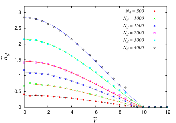
Figure 2: The effect of number of particles on the radial density is shown for the fixed value of $\Gamma_{g}=0.08$ and $\tilde{T}_{d}=0.10$. The symbols represent the data points from MD simulation whereas the curves represent the best fit of the corresponding data using trial function of the form given in right hand side of Eq.(21). It can be seen from the plot that the radius of dust cloud is almost independent of $N_{d}$ and any increases in the number of particle only increases the density of the core.

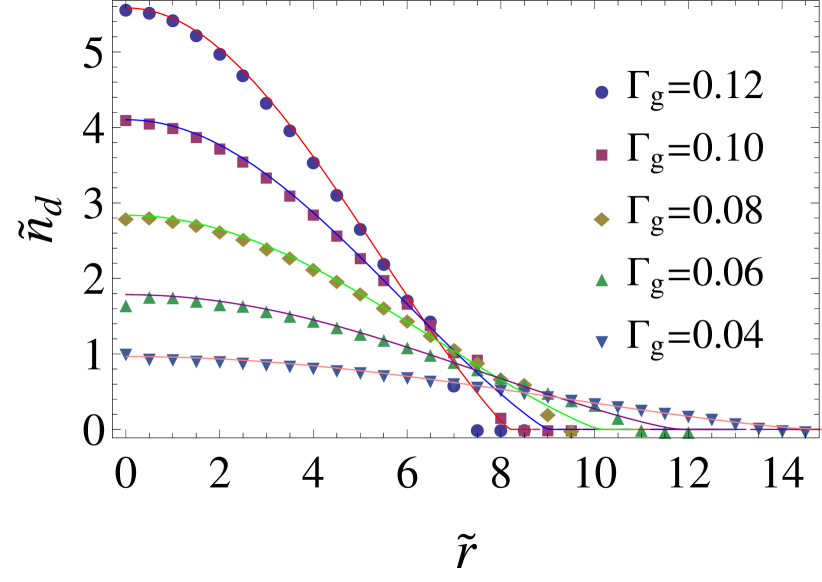
Figure 3: Effect of $\Gamma_{g}$ on the radial density profile: Radial density profile $\tilde{n}_{d}$ is plotted against the radial distance $\tilde{r}$ for different values of $\Gamma_{g}$ for the fixed $N_{d}=4000$ and $T_{d}=0.10$. The symbols represent the density profile obtained from the MD simulation whereas the solid lines correspond to the mean field solution of $\tilde{n}_{d}(\tilde{r})$ obtained from Eq.(17). It is clear from the results that the radius of the cloud $\tilde{R}$ decreases whereas the core density $\tilde{n}_{d0}$ increases with $\Gamma_{g}$.

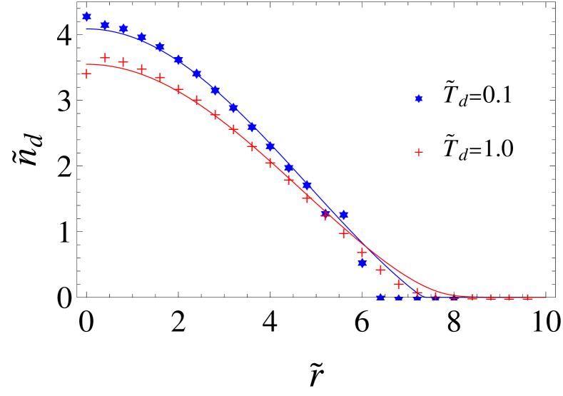
Figure 4: Effect of dust temperature on radial number density is shown for $\Gamma_{g}=0.15$ and $N_{d}=2000$ for $\tilde{T}_{d}=0.1$ and $\tilde{T}_{d}=1.0$. Symbols represent data points from the simulation whereas curves refer to the mean field solutions.

IV Simulation Results

The size of the cloud critically depends on three parameters, $N_{d}$, $\Gamma_{g}$ and $\tilde{T}_{d}$. Following these observations, the simulation results may broadly be divided into three parts accordingly; one, comprising the effect of $N_{d}$ on $\tilde{n}_{d}(\tilde{r})$ keeping $\Gamma_{g}$ and $\tilde{T}_{d}$ fixed, second, the effect of $\Gamma_{g}$ on $\tilde{n}_{d}$ for fixed $N_{d}$ and $\tilde{T}_{d}$ and third, the effect of $\tilde{T}_{d}$ on $\tilde{n}_{d}(\tilde{r})$ keeping $\Gamma_{g}$ and $N_{d}$ fixed.

IV.1 Effect of $N_{d}$ on density profile

To examine the effect of $N_{d}$ of $\tilde{n}_{d}(\tilde{r})$, we fix $\Gamma_{g}=0.08$ and $\tilde{T}_{d}=0.10$. The equilibrium radial density profile of dust cloud for different $N_{d}$ is shown by symbols in Fig.(2). It can be seen that as we increase the number of particles $N_{d}$ the central density (i.e. the density at $\tilde{r}=0$) increases whereas the radius of the cloud $\tilde{R}$ (value of $\tilde{r}$ at which $\tilde{n}_{d}=0$ ) is almost fixed. In other words, the dust cloud becomes denser with increase in the number of particle while size of the cloud is almost independent of the number of particles.

IV.2 Effect of $\Gamma_{g}$ on density profile

The effect of $\Gamma_{g}$ on radial number density $\tilde{n}_{d}(\tilde{r})$ for fixed number of particles $N_{d}=4000$ and constant temperature $T_{d}=0.10$ is shown in Fig.(3) where symbols represent the simulation data points and curves correspond to the mean field solution discussed in next section. It is clear from the Fig.(3), that the radial density, $\tilde{n}_{d}(\tilde{r})$, radius of the cloud, $\tilde{R}$ and central density, $\tilde{n}_{d0}$, depend on $\Gamma_{g}$.

IV.3 Effect of dust temperature on density profile

Effect of dust temperature on the radial density profile for $N_{d}=2000$ and $\Gamma_{g}=0.15$ is shown in Fig.(4). The equilibrium number density is plotted against radial distance for $\tilde{T}_{d}=0.1$ and $\tilde{T}_{d}=1.0$. It is seen that the central density of cloud decreases while radius increases with increase in temperature.

The observed simulation results can be explained in terms of mean field theoryAvinash and Shukla (2006); Avinash (2007a) described in the next section.

V Mean Field Solutions

In the mean field (continuum) limit, the electric force acting on the dust fluid behave like an effective ES pressure force. It can be seen as follows: In the zero correlation mean field limit, $Q_{d}\rightarrow 0$, $N_{d}\rightarrow\infty$ and $Q_{d}N_{d}=\text{finite}$, therefore, the double summation can be changed to smooth integrationAvinash (2010b) as $\sum_{i}^{N_{d}}\sum_{\hskip 2.84544ptj=1,\neq i}^{N_{d}}\rightarrow n_{d}N_{d}\int_{V_{d}}\;dV_{d}$. In this limit ES energy becomes;

$$U_{ES}=\frac{Q_{d}^{2}}{4\pi\epsilon_{0}}\frac{1}{2}\sum_{i}^{N_{d}}\sum_{\hskip 2.84544ptj=1,\neq i}^{N_{d}}\frac{\exp(-\kappa_{D}|r_{i}-r_{j}|)}{|r_{i}-r_{j}|}\rightarrow\frac{n_{d}N_{d}Q_{d}^{2}\lambda_{D}^{2}}{2\epsilon_{0}}.$$

Corresponding ES pressure can be obtained using the relation $P_{ES}=-\left({\partial U_{ES}}/{\partial V_{d}}\right)_{T_{d}}$ which comes out to be $P_{ES}={Q_{d}^{2}\lambda_{D}^{2}n_{d}^{2}}/{2\epsilon_{0}}$ suggesting that $P_{ES}\propto n_{d}^{2}$. The total dust pressure is the sum of kinetic pressure ($n_{d}T_{d}$) and ES pressureShukla et al. (2017). Similarly the gravitational force density, in the mean field limit, is given by $-m_{d}n_{d}\nabla\psi$ where $\psi$ is gravitational potential given by Poisson equation i.e.,

$$\nabla^{2}\psi=4\pi G\rho_{d}.$$ (10)

Therefore, equation of motion for such self-gravitating dust fluid is given by

$$\rho_{d}\frac{du_{d}}{dt}=-\nabla P_{d}-\rho_{d}\nabla\psi,$$ (11)

where $\rho_{d}(=m_{d}n_{d})$ is dust mass density, $P_{d}$ is total dust pressure (sum of kinetic pressure and ES pressure). In static equilibrium $u_{d}=0$, therefore

$$\nabla P_{d}=-\rho_{d}\nabla\psi.$$ (12)

Taking the divergence of Eq.(12) (after dividing by $\rho_{d}$) and using Eq.(10), we get

$$\nabla\cdot\left(\frac{\nabla P_{d}}{\rho_{d}}\right) = \nabla^{2}\psi$$ (13)

$$= 4\pi G\rho_{d},$$

The spherically symmetric force balance equation in the spherical polar coordinated becomes;

$$\frac{1}{r^{2}}\frac{d}{dr}\left(\frac{r^{2}}{m_{d}n_{d}}\frac{dP_{d}}{dr}\right)=-4\pi Gm_{d}n_{d},$$ (14)

where we still have to provide an equation of state for $P_{d}$ to close Eq. (14).

As our purpose is to compare the simulation results with the mean field solution, let us normalize Eq.(14) as we did in Sec.(III) where $r\rightarrow\tilde{r}\lambda_{D}$, $P_{d}\rightarrow\tilde{P}_{d}(\frac{Q_{d}^{2}}{4\pi\epsilon_{0}\lambda_{D}^{4}})$ and $n_{d}\rightarrow\tilde{n}_{d}/\lambda_{D}^{3}$. Therefore Eq. (14) becomes,

$$\frac{1}{\tilde{r}^{2}}\frac{d}{d\tilde{r}}\left(\frac{\tilde{r}^{2}}{\tilde{n}_{d}}\frac{d\tilde{P}_{d}}{d\tilde{r}}\right) = -\frac{4\pi Gm_{d}^{2}}{Q_{d}^{2}/4\pi\epsilon_{0}}\tilde{n}_{d}$$ (15)

$$= -4\pi\Gamma_{g}\tilde{n}_{d}.$$

Recently, Shukla et al Shukla et al. (2017) have obtained the equation of state for Yukawa fluid by using rigorous MD simulations. Their expression for total dust pressure in normalized units is given by

$$\tilde{P}_{d}=\tilde{n}_{d}\tilde{T}_{d}+\beta\>\tilde{n}_{d}^{2},$$ (16)

where $\tilde{T}_{d}$ is dust temperature and $\beta$ is a number of the order of $\pi$. In the expression of $\tilde{P}_{d}$, the first term which scales linearly with number density, is usual kinetic pressure term whereas second term which is proportional to the square of number density, corresponds to ES pressure. Substituting Eq.(16) in Eq.(15), we get the following differential equation

$$\tilde{n}_{d}^{\prime\prime}+\frac{\tilde{T}_{d}}{2\beta}\frac{\tilde{n}_{d}^{\prime\prime}}{\tilde{n}_{d}}+\frac{2}{r}\tilde{n}_{d}^{\prime}+\frac{\tilde{T}_{d}}{2\beta}\frac{2}{r}\frac{\tilde{n}_{d}^{\prime}}{\tilde{n}_{d}}-\frac{\tilde{T}_{d}}{2\beta}\frac{(\tilde{n}_{d}^{\prime})^{2}}{\tilde{n}_{d}^{2}}=-\frac{2\pi\Gamma_{g}}{\beta}\tilde{n}_{d}$$ (17)

where $\tilde{n}_{d}^{\prime}=d\tilde{n}_{d}/d\tilde{r}$ and $\tilde{n}_{d}^{\prime\prime}=d^{2}\tilde{n}_{d}/d\tilde{r}^{2}$. As Eq.(17) is a second order nonlinear differential equation, it requires two boundary conditions (BCs) for a unique solution which are given by;

$$\tilde{n}_{d}(0)=\tilde{n}_{d0},\hskip 12.80365pt\tilde{n}_{d}^{\prime}(0)=0.$$ (18)

Eq.(17) along with Eq.(18) may be solved numerically to get $\tilde{n}_{d}(\tilde{r})$ for a given temperature $\tilde{T}_{d}$, central density $\tilde{n}_{d0}$ and $\Gamma_{g}$. The radius of the cloud ($\tilde{R}$) is calculated using the relation $\tilde{n}_{d}(\tilde{R})=0$. whereas the mass of the cloud is obtained using the relation

$$M_{d}=m_{d}N_{d}=4\pi m_{d}\int_{0}^{R}\tilde{r}^{2}\tilde{n}_{d}(\tilde{r})d\tilde{r}.$$ (19)

Before comparing the MD results with the mean field solutions, we consider the special case of zero dust temperature in which Eq.(17) admits an exact analytic solution.

Special Case: Solution for $\mathbf{\tilde{T}_{d}=0}$

There is an interesting case in the limit $\tilde{T}_{d}=0$ when the Eq.(17) can be solved analyticallyAvinash and Shukla (2006). In this special case, the gravitation force is balanced completely by ES pressure force. In this limit Eq.(17) reduces to a linear differential equation given by;

$$\tilde{n}_{d}^{{}^{\prime\prime}}+\frac{2}{r}\tilde{n}_{d}^{{}^{\prime}}=-\frac{2\pi\Gamma_{g}}{\beta}\tilde{n}_{d}.$$ (20)

The solution of above differential equation along with BCs defined in Eq.(18), is given by

$$\tilde{n}_{d}(\tilde{r})=\tilde{n}_{d0}\frac{\sin\left(\sqrt{\frac{2\pi\Gamma_{g}}{\beta}}\;\tilde{r}\right)}{\left(\sqrt{\frac{2\pi\Gamma_{g}}{\beta}}\;\tilde{r}\right)}.$$ (21)

As mentioned earlier the radius of the cloud is obtained by setting $\tilde{n}_{d}(\tilde{R})=0$, which gives $\sqrt{\frac{2\pi\Gamma_{g}}{\beta}}\;R=\pi$. Therefore, radius of cloud is;

$$\tilde{R}=\sqrt{\frac{\pi\beta}{2\Gamma_{g}}}.$$ (22)

This should be noted that this radius is of the same order as obtained by equating average gravitational field to mean ES field discussed in Sec. I which gives the dust Jeans length ($L$ also provides the typical length scale of dust dispersion) as $L\sim\lambda_{D}\sqrt{1/\Gamma_{g}}$.

Relation between central density $\tilde{n}_{d}$ and $N_{d}$ can be obtained by integrating number density as follows

$$N_{d}=\int_{0}^{\tilde{R}}\tilde{n}_{d}(\tilde{r})4\pi\tilde{r}^{2}d\tilde{r}.$$ (23)

Substituting the value of $\tilde{n}_{d}$ and $\tilde{R}$ from Eq.(21) and (22) respectively in above equation gives,

$$\tilde{n}_{d0}=\frac{1}{\sqrt{2\pi}}\left(\frac{\Gamma_{g}}{\beta}\right)^{3/2}N_{d}$$ (24)

It should also be noted here that in the limit of $\tilde{T}_{d}\rightarrow 0$, the radius of the cloud $\tilde{R}$ is independent of the number of particles $N_{d}$ and is function of $\Gamma_{g}$ only [Eq.(22)] whereas $\tilde{n}_{d0}$ is directly proportion to $N_{d}$ and $\Gamma_{g}^{3/2}$ [Eq.(24)].

VI Validation of simulation with mean field solutions

The particle approach can be tested against the fluid approach by comparing MD results with the mean field solutions. Let’s compare them one by one.

In Sec. [IV.1] we have observed that the increase in $N_{d}$ does not affects the radius of cloud substantially but increases the density of cloud. A similar relation is seen in mean field solution in the limit $\tilde{T}_{d}\rightarrow 0$ through Eq. (22) and Eq. (24). Therefore, we fit our MD data for radial density profile in a trial function of the form given in Eq. (21),

$$\tilde{n}(r)=\tilde{n}_{d0}~{}\frac{\sin(kr)}{(kr)},$$

where parameters $\tilde{n}_{d0}$ and $k$ are obtained by least square fitting and are tabulated in Table. 1. The fitted curves are plotted along with simulation data in Fig. (2). It is clear from Table. 1 that value of $k$, which in mean field limit represents to $\sqrt{2\pi\Gamma_{g}/\beta}$, is constant under the numerical errors and so does the the radius of the cloud. Also, the constancy of $k$ or $\sqrt{2\pi\Gamma_{g}/\beta}\approx 0.315\pm 0.006$ fixes $\beta\approx 1.604\;\pi$. The Eq.(24) states that the central density $\tilde{n}_{d0}$ should be a linear function of $N_{d}$ and the predicted slope is $\frac{1}{\sqrt{2\pi}}\left(\frac{\Gamma_{g}}{\beta}\right)^{3/2}$ which comes out to be $7.98\times 10^{-4}$ for $\Gamma_{g}=0.08$ and $\beta=1.604\;\pi$. To verify Eq.(24), we fit central density vs. number of particles using data from Table 1. The slope of $\tilde{n}_{d0}$ vs. $N_{d}$ line comes out to be $(7.23\pm 0.07)\times 10^{-4}$ against the predicted value of $7.98\times 10^{-4}$ thereby validating the results with a deviation of about $10\%$ (Fig (5)).

Table 1: Equilibrium parameters for different $N_{d}$

$~{}~{}\mathbf{N_{d}}~{}~{}$	$~{}~{}~{}~{}\tilde{n}_{d0}~{}~{}~{}~{}~{}~{}$	k	$~{}~{}\tilde{R}=\pi/k~{}~{}$
500	$0.380\pm 0.003$	$0.321\pm 0.003$	$9.78\pm 0.09$
1000	$0.736\pm 0.008$	$0.316\pm 0.003$	$9.94\pm 0.09$
1500	$1.106\pm 0.009$	$0.317\pm 0.003$	$9.91\pm 0.09$
2000	$1.45\pm 0.01$	$0.315\pm 0.002$	$9.97\pm 0.06$
3000	$2.14\pm 0.01$	$0.313\pm 0.002$	$10.03\pm 0.06$
4000	$2.83\pm 0.02$	$0.312\pm 0.002$	$10.03\pm 0.06$

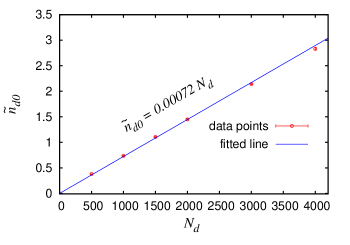
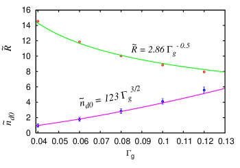
Figure 5: The density at the center of cloud, $\tilde{n}_{d0}$, is plotted against number of particles, $N_{d}$ in Fig.5. The $\tilde{n}_{d0}$ vs. $N_{d}$ plot is linear in nature and is consistent with Eq.(24). The dependence of $\tilde{n}_{d0}$ and size on parameters $\Gamma_{g}$ is shown in the Fig. 5.

The fitted parameters for different values of $\Gamma_{g}$ keeping $N_{d}$ and $T_{d}$ constant, are tabulated in Table 2. In the mean limit, the relation between $\tilde{R}$ and $\Gamma_{g}$, using Eq.(22), reduces to $\tilde{R}=2.813\;\Gamma_{g}^{-1/2}$ while relation between $\tilde{n}_{d0}$ and $\Gamma_{g}$, as predicted by Eq.(24), is given by $\tilde{n}_{d0}=141.07\;\Gamma_{g}^{3/2}$ (taking $N_{d}=4000$ and $\beta=1.60\;\pi$). A direct fit between $\Gamma_{g}$ and $\tilde{R}$ using Table 2 gives the relation $\tilde{R}=2.86\pm 0.02\;\Gamma_{g}^{-1/2}$ while relation between $\tilde{n}_{d0}$ and $\Gamma_{g}$ comes out to be $\tilde{n}_{d0}=123\pm 1\;\Gamma_{g}^{3/2}$ (Fig.(5)).

It should be noted that the parameters $\tilde{n}_{d0}$, $k$ shown in Table 1 and Table 2 are obtained by fitting the radial density data in the function $\tilde{n}(r)=\tilde{n}_{d0}\sin(kr)/(kr)$, which represents the mean field solution in the limit $\tilde{T}_{d}\rightarrow 0$. It is also noted that the simulation results at $T_{d}=0.1$ is a good approximation for analytic solutions at $T_{d}=0$. In Fig. (3) we plot the mean field solutions (solid curves) for different $\Gamma_{g}$ obtained by solving Eq.(17) with $\tilde{T}_{d}=0.10$. Simulation results agree well with mean field solutions for different $\Gamma_{g}$.

Table 2: Equilibrium parameters for different $\Gamma_{g}$

$~{}~{}\mathbf{\Gamma_{g}}~{}~{}$	$~{}~{}~{}~{}\tilde{n}_{d0}~{}~{}~{}~{}~{}~{}$	$~{}~{}~{}~{}~{}~{}k~{}~{}$	$~{}~{}\tilde{R}=\pi/k~{}~{}$
0.04	$0.965\pm 0.005$	$0.216\pm 0.001$	$14.54\pm 0.07$
0.06	$1.78\pm 0.01$	$0.265\pm 0.002$	$11.85\pm 0.09$
0.08	$2.84\pm 0.02$	$0.312\pm 0.002$	$10.04\pm 0.06$
0.10	$4.10\pm 0.04$	$0.355\pm 0.003$	$8.85\pm 0.07$
0.12	$5.58\pm 0.05$	$0.395\pm 0.004$	$7.95\pm 0.08$

To compare the effect of temperature in two approaches, we plot MD data (symbols) and the solution of Eq.(17) (curves) for different dust temperature as shown in Fig. (4). While plotting mean field solution, the central density is taken from simulation results and Eq.(17) is solved numerically. It can be seen from the plots that the mean field field solutions are validating simulation results.

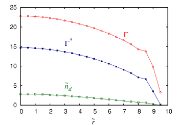
Figure 6: Typical values of the Coulomb coupling parameter $\Gamma$ and the coupling parameter $\Gamma^{*}\left(=\Gamma\exp(-\kappa)\right)$ corresponding to radial density profile $\tilde{n}_{d}(\tilde{r})$ is shown for $N_{d}=4000$ and $\Gamma_{g}=0.080$.

VII Summary and Conclusion

To summarize, we have examined the problem of equilibrium of self-gravitating dusty plasmas using particle level MD simulations. Dust grains interact with each other via repulsive Yukawa potential and attractive gravitational potential. The equilibrium of the system is characterized by three parameters, $\Gamma_{g}(=4\pi\epsilon_{0}Gm_{d}^{2}/Q_{d}^{2})$, number of particles $N_{d}$ and mean kinetic energy or temperature $\tilde{T}_{d}$ and depending upon these three parameters, different equilibrium structures are formed. The interior of these equilibrium structures is probed using radial density function where, center of mass of the cloud is taken as the $r=0$ point. We have also formulated the problem of equilibrium in the mean field limit where dust pressure, which is the sum of kinetic pressure and ES pressure, balances the self gravity. The results of mean field limit are compared with simulation results and the two approaches are found to be consistent with each other.

Our results predict that for the cold dust particles of constant charge and mass, the size of equilibrium structure is independent of number of particle in the cloud (or mass of the cloud). In fact, the addition of more number of particles results only in increasing the number density (or equivalently mass density) of the equilibrium cloud. Our results also predict that the equilibrium structures formed by the dust particles of relatively bigger size will be shorter in size and denser in nature. This happens because the increase in the dust size results in the increase of $\Gamma_{g}~{}(\text{which is a sensitive function of dust size as,}~{}\Gamma_{g}\propto r_{d}^{4}$) and the size of the equilibrium structure, $R\propto\lambda_{D}/\sqrt{\Gamma_{g}}\propto 1/r_{d}^{2}.$ The increase in temperature results in increasing the radius of equilibrium cloud. The effect of dust temperature is obvious. In our model, it is the sum of kinetic pressure and electrostatic pressure which balances the self-gravity and therefore, the increase in dust temperature implies an increase in kinetic pressure which ultimately pushes the dust grains outwards from the cloud, thereby increasing the size of the cloud.

It should be noted that the equation of state for ES pressure i.e. $P\propto n_{d}^{2}$ is derived with an assumption of weak coupling Avinash (2010a); Shukla et al. (2017), however, it may be very robust and could be valid in the strong coupling regime. For example, the mean field solution matches well even near the central region of dust cloud where dust is not weakly correlated and $\Gamma^{*}>1$ as shown in Fig. (6). Similar quadratic scaling of dust pressure is also observed in experiments on shock formation in a flowing 2D dusty plasma where Saitou et al. have shownSaitou et al. (2012) that the condition of shock formation is satisfied by equation of state $P_{d}\propto n_{d}^{\gamma}$ where $\gamma\simeq 2.2$. Some other examples where quadratic scaling is found to be valid in the even in the presence of correlations includes the simulations of Charan et al. where $P_{d}\propto n_{d}^{2}$ scaling is seen in the regions where dust particles are compressed by external gravity and dust is strongly coupledCharan et al. (2014). The simulation of Djouder et al. for dust monolayer confined by parabolic potential shows that the equation of state near zero dust temperature follows the relation $P_{d}\propto n_{d}^{2\sim 2.165}$ for a wide range of densities near the dust crystalDjouder et al. (2016).

We now briefly discuss the astrophysical significance of our results. The observations in the infrared region of spectrum have shown the evidences of dust overabundance inside the HII regions as compared to the interstellar mediumPanagia (1974); Tenorio-Tagle (1974). The length scale of these over dense clumps is below 1 pc to several AUs (1 pc $=3\times 10^{16}$ m, 1 AU $=1.5\times 10^{11}$ m).The origin of these structures is not known even today. We propose that the equilibrium structures discussed in our paper could be a possible candidate for these small scale structures observed in the HII region and interstellar medium. In our model the typical length scale of these structures is given by $R=\lambda_{D}/\sqrt{\Gamma_{g}}$. For the parameters of HII region: plasma density $n_{0}=10/$ c.c. (=$10^{7}\text{m}^{-3}$), $T=5000$ K and average dust size $\approx 0.3\;\mu$m we obtain $R\approx 3\times 10^{11}$ m which is roughly of the size of finest structure of clumps of gas and dust detected in interstellar medium Quirrenbach et al. (1989); Braun and Kanekar (2005); Smith et al. (2012). The equilibrium structures discussed in this paper could also be the precursor to a proto-planetary or proto-stellar core formation. For example, if the electric fields become weak over a period of time then these aggregates will slowly contract and become denser to give rise to van der Waals correlations and the formation of a more solid bodyAvinash and Shukla (2006).

It should also be noted that while formulating the problem of equilibrium, dust charge is taken to be constant and independent of number density while there are enough evidences to conform that charge of dust decreases with number density Havnes et al. (1990); Avinash et al. (2003); Barkan et al. (1994). As mentioned in Sec.I the reduction of dust charge at high density can limit the total mass supported by the ES pressure. Therefore our study is useful to the scenarios where dust density is low and dust charge is constant. A number of other effects like magnetic field, dust rotation etc. are also not taken into account and will be addressed in future communication.