Inference for ergodic diffusions plus noise

Abstract

We research adaptive maximum likelihood-type estimation for an ergodic diffusion process where the observation is contaminated by noise. This methodology leads to the asymptotic independence of the estimators for the variance of observation noise, the diffusion parameter and the drift one of the latent diffusion process. Moreover, it can lessen the computational burden compared to simultaneous maximum likelihood-type estimation. In addition to adaptive estimation, we propose a test to see if noise exists or not, and analyse real data as the example such that data contains observation noise with statistical significance.

1 Introduction

We consider a $d$-dimensional ergodic diffusion process defined by the following stochastic differential equation

$$\mathrm{d}X_{t}=b(X_{t},\beta)\mathrm{d}t+a(X_{t},\alpha)\mathrm{d}w_{t},\ X_{0}=x_{0},$$ (1)

where $\left\{w_{t}\right\}_{t\geq 0}$ is a $r$-dimensional standard Wiener process, $x_{0}$ is a $\mathbf{R}^{d}$-valued random variable independent of $\left\{w_{t}\right\}_{t\geq 0}$, $\alpha\in\Theta_{1}\subset\mathbf{R}^{m_{1}}$, $\beta\in\Theta_{2}\subset\mathbf{R}^{m_{2}}$ with $\Theta_{1}$ and $\Theta_{2}$ being compact and convex. Moreover, $b:\mathbf{R}^{d}\times\Theta_{2}\to\mathbf{R}^{d}$, $a:\mathbf{R}^{d}\times\Theta_{1}\to\mathbf{R}^{d}\otimes\mathbf{R}^{r}$ are known functions. We denote $\theta:=(\alpha,\beta)\in\Theta_{1}\times\Theta_{2}=:\Theta$ and $\theta^{\star}=(\alpha^{\star},\beta^{\star})$ as the true value of $\theta$ which belongs to $\mathrm{Int}(\Theta)$.

We deal with the problem of parametric inference for $\theta$ with $\left\{Y_{ih_{n}}\right\}_{i=1,\ldots,n}$ defined by the following model

$$Y_{ih_{n}}=X_{ih_{n}}+\Lambda^{1/2}\varepsilon_{ih_{n}},\ i=0,\ldots,n,$$ (2)

where $h_{n}>0$ is the discretisation step, $\Lambda\in\mathbf{R}^{d}\otimes\mathbf{R}^{d}$ is a positive semi-definite matrix and $\left\{\varepsilon_{ih_{n}}\right\}_{i=1,\ldots,n}$ is an i.i.d. sequence of $\mathbf{R}^{d}$-valued random variables such that $\mathbf{E}\left[{\varepsilon_{ih_{n}}}\right]=\mathbf{0}$, $\mathrm{Var}\left({\varepsilon_{ih_{n}}}\right)=I_{d}$, and each component is independent of other components, $\left\{{w_{t}}\right\}$ and $x_{0}$. Hence the term $\Lambda^{1/2}\varepsilon_{ih_{n}}$ indicates the exogenous noise. Let $\Theta_{\varepsilon}\in\mathbf{R}^{d(d+1)/2}$ be the convex and compact parameter space such that $\theta_{\varepsilon}:=\mathrm{vech}(\Lambda)\in\Theta_{\varepsilon}$ and $\Lambda_{\star}$ be the true value of $\Lambda$ such that $\theta_{\varepsilon}^{\star}:=\mathrm{vech}(\Lambda_{\star})\in\mathrm{Int}(\Theta_{\varepsilon})$, where $\mathrm{vech}$ is the half-vectorisation operator. We denote $\vartheta:=(\theta,\theta_{\varepsilon})$ and $\Xi:=\Theta\times\Theta_{\varepsilon}$. With respect to the sampling scheme, we assume that $h_{n}\to 0$ and $nh_{n}\to\infty$ as $n\to\infty$.

Our main concern with these settings is the adaptive maximum likelihood (ML)-type estimation scheme in the form of $\hat{\Lambda}_{n}=\frac{1}{2n}\sum_{i=0}^{n-1}\left({Y_{(i+1)h_{n}}-Y_{ih_{n}}}\right)^{\otimes 2}$,

$$\mathbb{H}_{1,n}^{\tau}(\hat{\alpha}_{n}|\hat{\Lambda}_{n}) =\sup_{\alpha\in\Theta_{1}}\mathbb{H}_{1,n}^{\tau}(\alpha|\hat{\Lambda}_{n}),$$ (3)

$$\mathbb{H}_{2,n}(\hat{\beta}_{n}|\hat{\alpha}_{n}) =\sup_{\beta\in\Theta_{2}}\mathbb{H}_{2,n}(\beta|\hat{\alpha}_{n}),$$ (4)

where $A^{\otimes 2}=AA^{T}$ for any matrix $A$, $A^{T}$ indicates the transpose of $A$, $\mathbb{H}_{1,n}^{\tau}$ and $\mathbb{H}_{2,n}$ are quasi-likelihood functions, which are defined in Section 3.

The composition of the model above is quite analogous to that of discrete-time state space models (e.g., see [19]) in terms of expression of endogenous perturbation in the system of interest and exogenous noise attributed to observation separately. As seen in the assumption $h_{n}\to 0$, this model that we consider is for the situation where high-frequency observation holds, and this requirement enhances the flexibility of modelling since our setting includes the models with non-linearity, dependency of the innovation on state space itself. In addition, adaptive estimation which also becomes possible through the high-frequency setting has the advantage in easing computational burden in comparison to simultaneous one. Fortunately, the number of situations where requirements are satisfied has been grown gradually, and will continue to soar because of increase in the amount of real-time data and progress of observation technology these days.

The idea of modelling with diffusion process concerning observational noise is no new phenomenon. For instance, in the context of high-frequency financial data analysis, the researchers have addressed the existence of ”microstructure noise” with large variance with respect to time increment questioning the premise that what we observe are purely diffusions. The energetic research of the modelling with ”diffusion + noise” has been conducted in the decade: some research have examined the asymptotics of this model in the framework of fixed time interval such that $nh_{n}=1$ (e.g., [9], [10], [12], [20] and [18]); and [3] and [4] research the parametric inference of this model with ergodicity and the asymptotic framework ${nh_{n}}\to\infty$. For parametric estimation for discretely observed diffusion processes without measurement errors, see [5], [24], [25], [2], [14] and references therein.

Our research is focused on the statistical inference for an ergodic diffusion plus noise. We give the estimation methodology with adaptive estimation that relaxes computational burden and that has been researched for ergodic diffusions so far (see [24], [25], [13], [21], [22]) in comparison to the simultaneous estimation of [3] and [4]. In previous researches the simultaneous asymptotic normality of $\hat{\Lambda}_{n}$, $\hat{\alpha}_{n}$ and $\hat{\beta}_{n}$ has not been shown, but our method allows us to see asymptotic normality and asymptotic independence of them with the different convergence rates. Our methods also broaden the applicability of modelling with stochastic differential equations since it is more robust for the existence of noise than the existent results in discretely observed diffusion processes with ergodicity not concerning observation noise.

As the real data analysis, we analyse the 2-dimensional wind data [17] and try to model the dynamics with 2-dimensional Ornstein-Uhlenbeck process. We utilise the fitting of our diffusion-plus-noise modelling and that of diffusion modelling with estimation methodology called local Gaussian approximation method (LGA method) which has been investigated for these decades (for instance, see [24], [13] and [14]). The result (see Section 5) seems that there is considerable difference between these estimates: however, we cannot evaluate which is the more trustworthy fitting only with these results. It results from the fact that we cannot distinguish a diffusion from a diffusion-plus-noise; if $\Lambda_{\star}=O$, then the observation is not contaminated by noise and the estimation of LGA should be adopted for its asymptotic efficiency; but if $\Lambda_{\star}\neq O$, what we observe is no more a diffusion process and the LGA method loses its theoretical validity. Therefore, it is necessary to compose the statistical hypothesis test with $H_{0}:\Lambda=O$ and $H_{1}:\Lambda\neq O$. In addition to estimation methodology, we also research this problem of hypothesis test and propose a test which has the consistency property.

In Section 2, we gather the assumption and notation across the paper. Section 3 gives the main results of this paper. Section 4 examines the result of Section 3 with simulation. In Section 5 we analyse the real data for wind velocity named MetData with our estimators and LGA as discussed above and test whether noise does exist.

2 Local means, notations and assumptions

2.1 Local means

We partition the observation into $k_{n}$ blocks containing $p_{n}$ observations and examine the property of the following local means such that

$$\bar{Z}_{j}{}=\frac{1}{p_{n}}\sum_{i=0}^{p_{n}-1}Z_{j\Delta_{n}+ih_{n}},\ j=0,\ldots,k_{n}-1,$$ (5)

where $\left\{{Z_{ih_{n}}}\right\}_{i=1,\ldots,n}$ is an arbitrary sequence of random variables on the mesh $\{ih_{n}\}_{i}$ as $\left\{{Y_{ih_{n}}}\right\}_{i=1,\ldots,n}$, $\left\{{X_{ih_{n}}}\right\}_{i=1,\ldots,n}$ and $\left\{{\varepsilon_{ih_{n}}}\right\}_{i=1,\ldots,n}$; and $\Delta_{n}=p_{n}h_{n}$. Note that $k_{n}p_{n}=n$ and $k_{n}\Delta_{n}=nh_{n}$.

In the same way as [3] and [4], our estimation method is based on these local means with respect to the observation $\left\{{Y_{ih_{n}}}\right\}_{i=1,\ldots,n}$. The idea is so straightforward; taking means of the data $\left\{{Y_{ih_{n}}}\right\}$ in each partition should reduce the influence of the noise term $\left\{{\varepsilon_{ih_{n}}}\right\}$ because of the law of large numbers and then we will obtain the information of the latent process $\left\{{X_{ih_{n}}}\right\}$.

We show how local means work to extract the information of the latent process. The first plot on next page (Figure 3) is the simulation of a 1-dimensional Ornstein-Uhlenbeck process such that

$$\mathrm{d}X_{t}=-\left({X_{t}-1}\right)\mathrm{d}t+\mathrm{d}w_{t},X_{0}=1$$ (6)

where $r=1$, $n=10^{4}$ and $h_{n}=n^{-0.7}$. Secondly, we contaminate the observation with normally-distributed noise $\left\{{\varepsilon_{ih_{n}}}\right\}$ and $\Lambda_{\star}=0.1$ and plot the observation on next page (Figure 3). Finally we make the sequence of local means $\left\{{\bar{Y}_{j}}\right\}$ where $p_{n}=25$ and $k_{n}=400$ plot at the bottom of the next page (Figure 3).

With these plots, it seems that the local means recover rough states of the latent processes, and actually it is possible to compose the quantity which converges to each state $\left\{{X_{j\Delta_{n}}}\right\}$ on the mesh $\left\{{j\Delta_{n}}\right\}$ for Proposition 12 with the assumptions below.

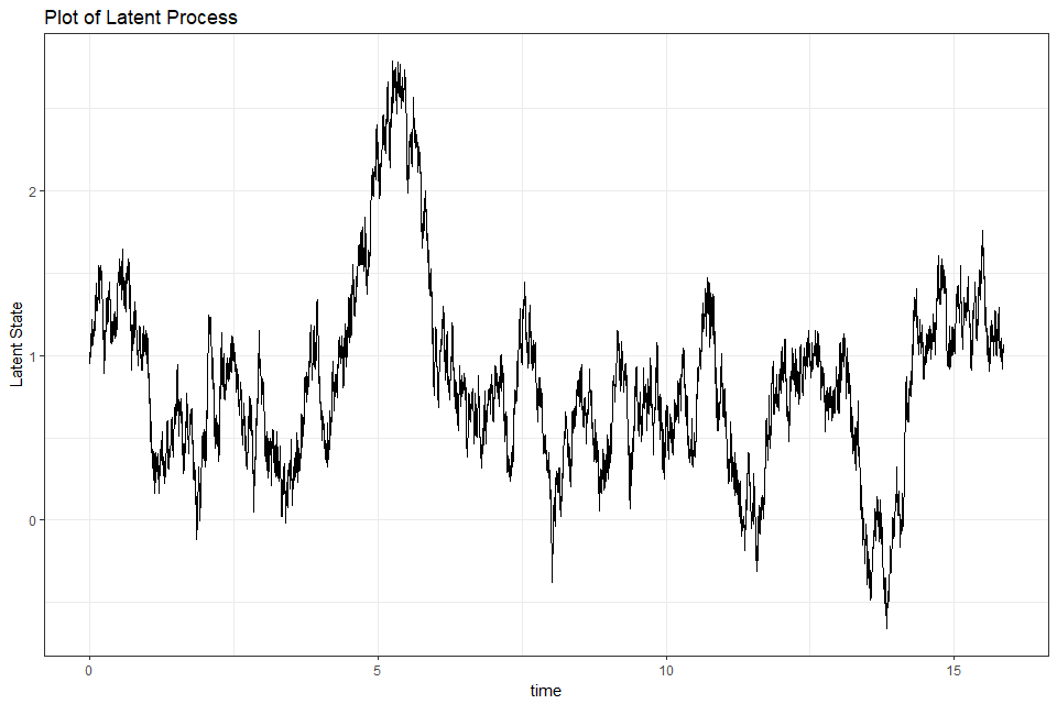
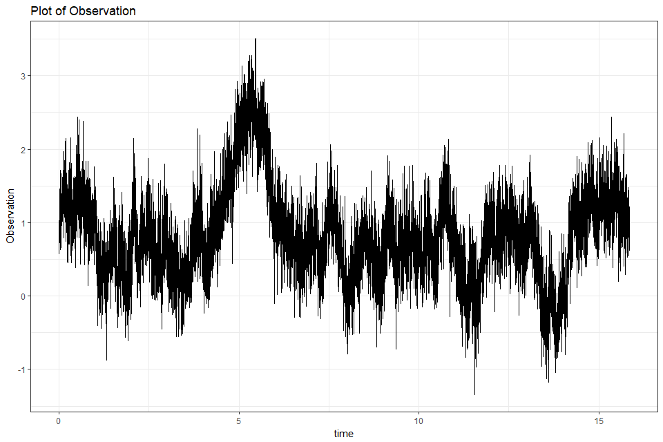
Figure 1: plot of the latent process

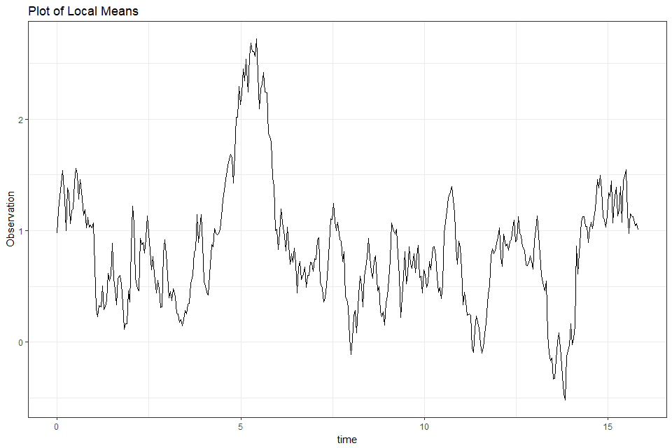
Figure 2: plot of the contaminated observation

Figure 3: plot of the local means

2.2 Notations and assumptions

We set the following notations.

1. For a matrix $A$, $A^{T}$ denotes the transpose of $A$ and $A^{\otimes 2}:=AA^{T}$. For same size matrices $A$ and $B$, $A\left\llbracket B\right\rrbracket:=\mathrm{tr}\left({AB^{T}}\right)$.

2. For any vector $v$, $v^{(i)}$ denotes the $i$-th component of $v$. Similarly, $M^{(i,j)}$, $M^{(i,\cdot)}$ and $M^{(\cdot,j)}$ denote the $(i,j)$-th component, the $i$-th row vector and $j$-th column vector of a matrix $M$ respectively.

3. For any vector $v$, $\left\|{v}\right\|:=\sqrt{\sum_{i}\left({v^{(i)}}\right)^{2}}$, and for any matrix $M$, $\left\|{M}\right\|:=\sqrt{\sum_{i,j}\left({M^{(i,j)}}\right)^{2}}$.

4. $A(x,\alpha):=\left({a(x,\alpha)}\right)^{\otimes 2}.$

5. $C$ is a positive generic constant independent of all other variables. If it depends on fixed other variables, e.g. an integer $k$, we will express as $C(k)$.

6. $a(x):=a(x,\alpha^{\star})$ and $b(x):=b(x,\beta^{\star})$.

7. Let us define $\vartheta:=\left({\theta,\theta_{\varepsilon}}\right)\in\Xi$.

8. A $\mathbf{R}$-valued function $f$ on $\mathbf{R}^{d}$ is a polynomial growth function if for all $x\in\mathbf{R}^{d}$,

   $$\left|{f(x)}\right|\leq C\left({1+\left\|{x}\right\|}\right)^{C}.$$

   $g:\mathbf{R}^{d}\times\Theta\to\mathbf{R}$ is a polynomial growth function uniformly in $\theta\in\Theta$ if for all $x\in\mathbf{R}^{d}$,

   $$\sup_{\theta\in\Theta}\left|{g(x,\theta)}\right|\leq C\left({1+\left\|{x}\right\|}\right)^{C}.$$

   Similarly we say $h:\mathbf{R}^{d}\times\Xi\to\mathbf{R}$ is a polynomial growth function uniformly in $\vartheta\in\Xi$ if for all $x\in\mathbf{R}^{d}$,

   $$\sup_{\vartheta\in\Xi}\left|{h(x,\vartheta)}\right|\leq C\left({1+\left\|{x}\right\|}\right)^{C}.$$

9. Let us denote for any $\mu$-integrable function $f$ on $\mathbf{R}^{d}$, $\mu(f(\cdot)):=\int f(x)\mu(\mathrm{d}x).$

10. We set

    $$\mathbb{Y}_{1}^{\tau}(\alpha) :=-\frac{1}{2}\nu_{0}\left({\mathrm{tr}\left({\left({A^{\tau}(\cdot,\alpha,\Lambda_{\star})}\right)^{-1}A^{\tau}(\cdot,\alpha^{\star},\Lambda_{\star})-I_{d}}\right)+\log\frac{\det A^{\tau}(\cdot,\alpha,\Lambda_{\star})}{\det A^{\tau}(\cdot,\alpha^{\star},\Lambda_{\star})}}\right),$$

    $$\mathbb{Y}_{2}(\beta) :=-\frac{1}{2}\nu_{0}\left({\left({A(\cdot,\alpha^{\star})}\right)^{-1}\left\llbracket\left({b(\cdot,\beta)-b(\cdot,\beta^{\star})}\right)^{\otimes 2}\right\rrbracket}\right),$$

    where $A^{\tau}(\cdot,\alpha,\Lambda):=A(\cdot,\alpha)+3\Lambda\mathbf{1}_{\left\{2\right\}}\left(\tau\right)$ and $\nu_{0}$ is the invariant measure of $X$.

11. Let

    $$\left\{B_{\kappa}(x)\left|\kappa=1,\ldots,m_{1},\ B_{\kappa}=(B_{\kappa}^{(j_{1},j_{2})})_{j_{1},j_{2}}\right.\right\},$$

    $$\left\{f_{\lambda}(x)\left|\lambda=1,\ldots,m_{2},\ f_{\lambda}=(f^{(1)}_{\lambda},\ldots,f^{(d)}_{\lambda})\right.\right\}$$

    be sequences of $\mathbf{R}^{d}\otimes\mathbf{R}^{d}$-valued functions and $\mathbf{R}^{d}$-valued ones respectively such that the components of themselves and their derivative with respect to $x$ are polynomial growth functions for all $\kappa$ and $\lambda$. Then we define the following matrix

    $$W_{1}^{(l_{1},l_{2}),(l_{3},l_{4})} :=\sum_{k=1}^{d}\left({\Lambda_{\star}^{1/2}}\right)^{(l_{1},k)}\left({\Lambda_{\star}^{1/2}}\right)^{(l_{2},k)}\left({\Lambda_{\star}^{1/2}}\right)^{(l_{3},k)}\left({\Lambda_{\star}^{1/2}}\right)^{(l_{4},k)}\left({\mathbf{E}\left[{\left|{\varepsilon_{0}^{k}}\right|^{4}}\right]-3}\right)$$

    $$\qquad+\frac{3}{2}\left({\Lambda_{\star}^{(l_{1},l_{3})}\Lambda_{\star}^{(l_{2},l_{4})}+\Lambda_{\star}^{(l_{1},l_{4})}\Lambda_{\star}^{(l_{2},l_{3})}}\right),$$

    and matrix-valued functionals, for $\bar{B}_{\kappa}:=\frac{1}{2}\left({B_{\kappa}+B_{\kappa}^{T}}\right)$,

    $$\left({W_{2}^{(\tau)}(\left\{{B_{\kappa}}\right\})}\right)^{(\kappa_{1},\kappa_{2})} :=\begin{cases}\nu_{0}\left({\mathrm{tr}\left\{{\left({\bar{B}_{\kappa_{1}}A\bar{B}_{\kappa_{2}}A}\right)(\cdot)}\right\}}\right)\\ \qquad\text{ if }\tau\in(1,2),\\ \nu_{0}\left({\mathrm{tr}\left\{{\left({\bar{B}_{\kappa_{1}}A\bar{B}_{\kappa_{2}}A+4\bar{B}_{\kappa_{1}}A\bar{B}_{\kappa_{2}}\Lambda_{\star}+12\bar{B}_{\kappa_{1}}\Lambda_{\star}\bar{B}_{\kappa_{2}}\Lambda_{\star}}\right)(\cdot)}\right\}}\right)\\ \qquad\text{ if }\tau=2,\end{cases}$$

    $$\left({W_{3}(\left\{{f_{\lambda}}\right\})}\right)^{(\lambda_{1},\lambda_{2})} :=\nu_{0}\left({\left({f_{\lambda_{1}}A\left({f_{\lambda_{2}}}\right)^{T}}\right)(\cdot)}\right).$$

12. $\overset{P}{\to}$ and $\overset{\mathcal{L}}{\to}$ indicate convergence in probability and convergence in law respectively.

13. For $f(x)$, $g(x,\theta)$ and $h(x,\vartheta)$, $f^{\prime}(x):=\frac{\mathrm{d}}{\mathrm{d}x}f(x)$, $f^{\prime\prime}(x):=\frac{\mathrm{d}^{2}}{\mathrm{d}x^{2}}f(x)$, $\partial_{x}g(x,\theta):=\frac{\partial}{\partial x}g(x,\theta)$, $\partial_{\theta}g(x,\theta):=\frac{\partial}{\partial\theta}g(x,\theta)$, $\partial_{x}h(x,\vartheta):=\frac{\partial}{\partial x}h(x,\vartheta)$ and $\partial_{\vartheta}h(x,\vartheta):=\frac{\partial}{\partial\vartheta}h(x,\vartheta)$.

We make the following assumptions.

1. $b$ and $a$ are continuously differentiable for 4 times, and the components of themselves as well as their derivatives are polynomial growth functions uniformly in $\theta\in\Theta$. Furthermore, there exists $C>0$ such that for all $x\in\mathbf{R}^{d}$,

   $$\left\|{b(x)}\right\|+\left\|{b^{\prime}(x)}\right\|+\left\|{b^{\prime\prime}(x)}\right\|\leq C(1+\left\|{x}\right\|),$$

   $$\left\|{a(x)}\right\|+\left\|{a^{\prime}(x)}\right\|+\left\|{a^{\prime\prime}(x)}\right\|\leq C(1+\left\|{x}\right\|).$$

2. $X$ is ergodic and the invariant measure $\nu_{0}$ has $k$-th moment for all $k>0$.

3. For all $k>0$, $\sup_{t\geq 0}\mathbf{E}\left[{\left\|{X_{t}}\right\|^{k}}\right]<\infty$.

4. For any $k>0$, $\varepsilon_{ih_{n}}$ has $k$-th moment and the component of $\varepsilon_{ih_{n}}$ are independent of the other components for all $i$, $\left\{{w_{t}}\right\}$ and $x_{0}$. In addition, the marginal distribution of each component is symmetric.

5. $\inf_{x,\alpha}\det c(x,\alpha)>0$.

6. There exist $\chi>0$ and $\tilde{\chi}>0$ such that for all $\tau$, $\alpha$ and $\beta$, $\mathbb{Y}_{1}^{\tau}(\alpha)\leq-\chi\left\|{\alpha-\alpha^{\star}}\right\|^{2}$, and $\mathbb{Y}_{2}^{\tau}(\beta)\leq-\tilde{\chi}\left\|{\beta-\beta^{\star}}\right\|^{2}$.

7. The components of $b$, $a$, $\partial_{x}b$, $\partial_{\beta}b$, $\partial_{x}a$, $\partial_{\alpha}a$, $\partial_{x}^{2}b$, $\partial_{\beta}^{2}b$, $\partial_{x}\partial_{\beta}b$, $\partial_{x}^{2}a$, $\partial_{\alpha}^{2}a$ and $\partial_{x}\partial_{\alpha}a$ are polynomial growth functions uniformly in $\theta\in\Theta$.

8. $h_{n}=p_{n}^{-\tau},\ \tau\in(1,2]$ and $h_{n}\to 0$, $p_{n}\to\infty$, $k_{n}\to\infty$, $\Delta_{n}=p_{n}h_{n}\to 0$, $nh_{n}\to\infty$ as $n\to\infty$.

9. If the index set $\mathcal{K}:=\left\{{i\in\left\{{1,\ldots,d}\right\}:\Lambda_{\star}^{(i,i)}>0}\right\}$ is not null, then the submatrix of $\Lambda_{\star}$ such that $\Lambda_{\star,\mathrm{sub}}:=\left[{\Lambda_{\star}^{(i_{1},i_{2})}}\right]_{i_{1},i_{2}\in\mathcal{K}}$ is positive definite.

Remark 1.

Some of the assumptions are ordinary ones in statistical inference for ergodic diffusions: (A1) and (A7) which indicates local Lipschitz continuity lead to existence and uniqueness of the solution of the stochastic differential equation. (A2), (A3) and (A5) can be seen in the literature such as [14] and some sufficient conditions are shown in [21]. (A6) is the identifiability condition adopted in [21] and [25], supporting non-degeneracy of information matrices simultaneously.

(A4) is a stronger assumption with respect to integrability of $\left\{\varepsilon_{ih_{n}}\right\}_{i=0,\ldots,n}$ compared to [3] and [4]. We consider multi-dimensional parameters in variance of noise, the diffusion coefficient and the drift one, and it results in the necessity of stronger integrability of $\varepsilon_{ih_{n}}$ when we prove Theorem 17, which shows that some empirical functionals uniformly converge to 0 in probability.

3 Main results

3.1 Adaptive ML-type estimation

Firstly, we construct an estimator for $\Lambda$ such that $\hat{\Lambda}_{n}:=\frac{1}{2n}\sum_{i=0}^{n-1}\left({Y_{(i+1)h_{n}}-Y_{ih_{n}}}\right)^{\otimes 2}$, which takes the form similar to the quadratic variation of $\left\{Y_{ih_{n}}\right\}_{i=0,\ldots,n}$.

Lemma 1.

Under (A1)-(A4), $h_{n}\to 0$ and $nh_{n}\to\infty$ as $n\to\infty$, $\hat{\Lambda}_{n}$ is consistent.

Remark 2.

The result of Lemma 1 can be understood intuitively: note the order evaluation $\sum_{i=0}^{n-1}\left(X_{\left(i+1\right)h_{n}}-X_{ih_{n}}\right)^{\otimes 2}=O_{P}\left(nh_{n}\right)$ and $\sum_{i=0}^{n-1}\left(\varepsilon_{\left(i+1\right)h_{n}}-\varepsilon_{ih_{n}}\right)^{\otimes 2}=O_{P}\left(n\right)$; and the cross term being merely a residual because of independence of $\left\{X_{t}\right\}_{t\geq 0}$ and $\left\{\varepsilon_{ih_{n}}\right\}_{i=0,\ldots,n}$.

We propose the following Gaussian-type quasi-likelihood functions such that

$$\mathbb{H}_{1,n}^{\tau}(\alpha|\Lambda):=-\frac{1}{2}\sum_{j=1}^{k_{n}-2}\left({\left({\frac{2}{3}\Delta_{n}A_{n}^{\tau}(\bar{Y}_{j-1},\alpha,\Lambda)}\right)^{-1}\left\llbracket\left({\bar{Y}_{j+1}-\bar{Y}_{j}}\right)^{\otimes 2}\right\rrbracket+\log\det\left({A_{n}^{\tau}(\bar{Y}_{j-1},\alpha,\Lambda)}\right)}\right),$$ (7)

$$\mathbb{H}_{2,n}(\beta|\alpha):=-\frac{1}{2}\sum_{j=1}^{k_{n}-2}\left({\Delta_{n}A(\bar{Y}_{j-1},\alpha)}\right)^{-1}\left\llbracket\left({\bar{Y}_{j+1}-\bar{Y}_{j}-\Delta_{n}b(\bar{Y}_{j-1},\beta)}\right)^{\otimes 2}\right\rrbracket,$$ (8)

where $A_{n}^{\tau}(x,\alpha,\Lambda):=A(x,\alpha)+3\Delta_{n}^{\frac{2-\tau}{\tau-1}}\Lambda$. They are quite similar to the quasi-likelihood functions for discretely-observed ergodic diffusion processes where $nh_{n}^{2}\to 0$ proposed by [21] except for the scaling $2/3$ seen in $\mathbb{H}_{1,n}^{\tau}$. It is because

$$\mathbf{E}\left[\left(\bar{Y}_{j+1}-\bar{Y}_{j}\right)^{\otimes 2}|X_{j\Delta_{n}},\left\{\varepsilon_{ih_{n}}\right\}_{i=0,\ldots,jp_{n}-1}\right]\approx\frac{2}{3}\Delta_{n}A_{n}^{\tau}\left(X_{j\Delta_{n}},\alpha^{\star},\Lambda_{\star}\right)$$ (9)

in some sense (see Proposition 13 or Theorem 18), which can be contrasted with that $\mathbf{E}\left[\left(X_{\left(i+1\right)h_{n}}-X_{ih_{n}}\right)^{\otimes 2}|X_{ih_{n}}\right]\approx h_{n}A\left(X_{ih_{n}},\alpha^{\star}\right)$. We define the adaptive ML-type estimators $\hat{\alpha}_{n}$ and $\hat{\beta}_{n}$ corresponding to $\mathbb{H}_{1,n}^{\tau}$ and $\mathbb{H}_{2,n}$, where

$$\mathbb{H}_{1,n}^{\tau}(\hat{\alpha}_{n}|\hat{\Lambda}_{n}) =\sup_{\alpha\in\Theta_{1}}\mathbb{H}_{1,n}^{\tau}(\alpha|\hat{\Lambda}_{n}),$$ (10)

$$\mathbb{H}_{2,n}(\hat{\beta}_{n}|\hat{\alpha}_{n}) =\sup_{\beta\in\Theta_{2}}\mathbb{H}_{2,n}(\beta|\hat{\alpha}_{n}).$$ (11)

The consistency of these estimators is given by the next theorem.

Theorem 2.

Under (A1)-(A7) and (AH), $\hat{\alpha}_{n}$ and $\hat{\beta}_{n}$ are consistent.

Remark 3.

These adaptive ML-type estimators have the advantage that the computation burden in optimisation is reduced compared to that of simultaneous ML-type ones maximising the simultaneous quasi-likelihood $\mathbb{H}_{n}\left(\alpha,\beta|\Lambda\right)$ such that

$$\mathbb{H}_{n}\left(\hat{\alpha}_{n},\hat{\beta}_{n}|\hat{\Lambda}_{n}\right)=\sup_{\alpha\in\Theta_{1},\beta\in\Theta_{2}}\mathbb{H}_{n}\left(\alpha,\beta|\hat{\Lambda}_{n}\right)$$ (12)

studied in [3] and [4].

To argue the asymptotic normality of the estimators, let us denote the limiting information matrices

$$\mathcal{I}^{\tau}(\vartheta^{\star}) :=\mathrm{diag}\left\{W_{1},\mathcal{I}^{(2,2),\tau},\mathcal{I}^{(3,3)}\right\}(\vartheta^{\star})$$ (13)

$$\mathcal{J}^{\tau}(\vartheta^{\star}) :=\mathrm{diag}\left\{I_{d(d+1)/2},\mathcal{J}^{(2,2),\tau},\mathcal{J}^{(3,3)}\right\}(\vartheta^{\star})$$ (14)

where for $i_{1},i_{2}\in\left\{{1,\ldots,m_{1}}\right\}$,

$$\mathcal{I}^{(2,2),\tau}(\vartheta^{\star}) :=W_{2}^{(\tau)}\left({\left\{{\frac{3}{4}\left({A^{\tau}}\right)^{-1}\left({\partial_{\alpha^{(k_{1})}}A}\right)\left({A^{\tau}}\right)^{-1}(\cdot,\vartheta^{\star})}\right\}_{k_{1}}}\right),$$ (15)

$$\mathcal{J}^{(2,2),\tau}(\vartheta^{\star}) :=\left[{\frac{1}{2}\nu_{0}\left({\mathrm{tr}\left\{{\left({A^{\tau}}\right)^{-1}\left({\partial_{\alpha^{(i_{1})}}A}\right)\left({A^{\tau}}\right)^{-1}\left({\partial_{\alpha^{(i_{2})}}A}\right)}\right\}(\cdot,\vartheta^{\star})}\right)}\right]_{i_{1},i_{2}},$$ (16)

which are the information for the diffusion parameter $\alpha$, and for $j_{1},j_{2}\in\left\{{1,\ldots,m_{2}}\right\}$,

$$\mathcal{I}^{(3,3)}(\theta^{\star}) =\mathcal{J}^{(3,3)}(\theta^{\star}):=\left[{\nu_{0}\left({\left({A}\right)^{-1}\left\llbracket\left({\partial_{\beta^{(j_{1})}}b}\right)\left({\partial_{\beta^{(j_{2})}}b}\right)^{T}\right\rrbracket(\cdot,\theta^{\star})}\right)}\right]_{j_{1},j_{2}}$$ (17)

which are that for the drift one $\beta$. To ease the notation, let us also denote $\hat{\theta}_{\varepsilon,n}:=\mathrm{vech}\hat{\Lambda}_{n}$ and $\theta_{\varepsilon}^{\star}:=\mathrm{vech}\Lambda_{\star}$.

Theorem 3.

Under (A1)-(A7), (AH) and $k_{n}\Delta_{n}^{2}\to 0$, the following convergence in distribution holds:

$$\left[\sqrt{n}\left(\hat{\theta}_{\varepsilon,n}-\theta_{\varepsilon}^{\star}\right),\ \sqrt{k_{n}}\left(\hat{\alpha}_{n}-\alpha^{\star}\right),\ \sqrt{nh_{n}}\left(\hat{\beta}_{n}-\beta^{\star}\right)\right]$$

$$\hskip 85.35826pt\overset{\mathcal{L}}{\to}N\left({\mathbf{0},\left({\mathcal{J}^{\tau}(\vartheta^{\star})}\right)^{-1}\mathcal{I}^{\tau}(\vartheta^{\star})\left({\mathcal{J}^{\tau}(\vartheta^{\star})}\right)^{-1}}\right).$$

This theorem shows the difference of the convergence rates with respect to $\hat{\theta}_{\varepsilon,n}$, $\hat{\alpha}_{n}$ and $\hat{\beta}_{n}$ which is essentially significant to construct adaptive estimation approach. The difference among these convergence rates can be intuitively comprehended: the estimator for $\Lambda$ has $\sqrt{n}$-consistency as ordinary i.i.d. case because it is estimated with the quadratic variation of observation masking the influence of the latent process $\left\{X_{t}\right\}_{t\geq 0}$ as noted in the remark for Lemma 1; $\hat{\alpha}$ which is estimated with the quasi-likelihoods composed by $k_{n}$ local means $\left\{\bar{Y}_{j}\right\}_{j=0,\ldots,k_{n}-1}$ has $\sqrt{k_{n}}$-consistency corresponding to $\sqrt{n}$-consistency in the inference for discretely-observed diffusion processes; and $\hat{\beta}_{n}$ has $\sqrt{nh_{n}}$-consistency which is ordinary in statistics for diffusion processes.

Note that our estimator $\hat{\beta}_{n}$ is asymptotically efficient for all $\tau\in\left(1,2\right]$: the limiting variance of $\sqrt{nh_{n}}\left(\hat{\beta}_{n}-\beta^{\star}\right)$ is the inverse of the Fisher information. It is because we construct adaptive quasi-likelihood functions for the diffusion parameter $\alpha$ and the drift one $\beta$ separately; to the contrary, a simultaneous quasi-likelihood functions proposed in [3] and [4] cannot achieve the asymptotic efficiency under $\tau=2$.

Remark 4.

(AH) inherits the assumption in both [3] and [4]. The tuning parameter $\tau$ controls the size and the number of partitions denoted as $p_{n}$ and $k_{n}$ given for observations, and for all $\tau\in\left(1,2\right]$ we have shown our estimators have asymptotic normality. It can be tuned to get optimal in each application, but the following discussion may give guide to determine $\tau$. Generally speaking, larger $\tau$ has an advantage in asymptotics of our estimators since higher $\tau$ indicates smaller $k_{n}\Delta_{n}^{2}$ whose convergence to 0 is one of the conditions to show asymptotic normality of the estimators. Let us consider the case where it holds $nh_{n}^{\gamma}\to 0$ for some $\gamma\in\left(1,3/2\right]$; then $k_{n}\Delta_{n}^{2}=nh_{n}^{2-1/\tau}\to 0$ if $\gamma>2-1/\tau$, which is the condition can be eased with larger $\tau$. On the other hand, there does not exist any $C>0$ such that $\mathcal{I}^{(2,2),\tau}=C\mathcal{J}^{(2,2),\tau}$ if $\tau=2$ which makes it difficult to compose test statistics like likelihood-ratio ones (see [16]). Hence in practice, $\tau$ sufficiently close to $2$ can be optimal, but it would be hard to discuss goodness-of-fit of models when $\tau=2$ exactly.

3.2 Test for noise detection

We formulate the statistical hypothesis test such that

$$H_{0}:\Lambda_{\star}=O,\ H_{1}:\Lambda_{\star}\neq O.$$

We define $S_{t}:=\sum_{l=1}^{d}X_{t}^{(l)}$ and $\mathscr{S}_{ih_{n}}:=\sum_{l=1}^{d}Y_{ih_{n}}^{(l)}$ and $\left[{X_{t}^{(1)},\ldots,X_{t}^{(d)},S_{t}}\right]$ is also an ergodic diffusion. Furthermore,

$$Z_{n}:=\sqrt{\frac{2p_{n}}{3\sum_{j=1}^{k_{n}-2}\left({\bar{\mathscr{S}}_{j+1}-\bar{\mathscr{S}}_{j}}\right)^{4}}}\left({\sum_{i=0}^{n-1}\left({\mathscr{S}_{(i+1)h_{n}}-\mathscr{S}_{ih_{n}}}\right)^{2}-\sum_{0\leq 2i\leq n-2}\left({\mathscr{S}_{(2i+2)h_{n}}-\mathscr{S}_{2ih_{n}}}\right)^{2}}\right),$$ (18)

where $\bar{\mathscr{S}}_{j}:=\frac{1}{p_{n}}\sum_{i=0}^{p_{n}-1}\mathscr{S}_{j\Delta_{n}+ih_{n}}$, and consider the hypothesis test with rejection region $Z_{n}\geq z_{\alpha}$ where $z_{\alpha}$ is the $(1-\alpha)$-quantile of $N(0,1)$.

Theorem 4.

Under $H_{0}$, (A1)-(A5), (AH) and $nh_{n}^{2}\to 0$,

$$Z_{n}\overset{\mathcal{L}}{\to}N(0,1).$$

Theorem 5.

Under $H_{1}$, (A1)-(A5), (AH), (T1) and $nh_{n}^{2}\to 0$, the test is consistent, i.e., for all $\alpha\in(0,1)$,

$$P(Z_{n}\geq z_{\alpha})\to 1.$$

Remark 5.

The consistency shown above utilises the well-known fact in financial econometrics that the quadratic variation of process as diverges to infinity as observation frequency increases when the observation is contaminated by exogenous noise. The first quadratic variation in the bracket of $Z_{n}$ composes of the entire observation, and the second one halves the number of samples with doubling the frequency from $h_{n}$ to $2h_{n}$. It results in that the first quadratic variation divided by $2n$ converges to $\sum_{\ell_{1}}\sum_{\ell_{2}}\Lambda_{\star}^{\left(\ell_{1},\ell_{2}\right)}$ in probability while the second one divided by $2n$ converges to $(1/2)\sum_{\ell_{1}}\sum_{\ell_{2}}\Lambda_{\star}^{\left(\ell_{1},\ell_{2}\right)}$ in probability. This difference is sufficiently large so that $Z_{n}$ diverges in the sense of $P\left(Z_{n}\geq z_{\alpha}\right)\to 1$ for any $\alpha\in(0,1)$.

In the next place, we concern approximation of the power in the finite sample scheme and consider the following sequence of alternatives

$$\left(\Lambda_{\star}\right)_{n}=\frac{h_{n}}{\sqrt{n}}\mathfrak{M},$$

where $\mathfrak{M}\geq 0$ and $\delta:=\sum_{\ell_{1}}\sum_{\ell_{2}}\mathfrak{M}^{\left(\ell_{1},\ell_{2}\right)}>0$. Then we obtain the next result for approximation of power.

Theorem 6.

Under the sequence of the alternatives $\left\{\left(\Lambda_{\star}\right)_{n}\right\}$, (A1)-(A5), (AH) and $nh_{n}^{2}\to 0$, the limit power of the test is $\Phi\left(\delta-z_{\alpha}\right)$.

Remark 6.

(i) The order of the alternatives above might seem to be peculiar, but can be comprehended as follows: the convergence in distribution in Theorem 4 can result from that of the following quantity

$$\sqrt{n}\left(\frac{1}{nh_{n}}\sum_{i=0}^{n-1}\left(S_{\left(i+1\right)h_{n}}-S_{ih_{n}}\right)^{2}-\frac{1}{nh_{n}}\sum_{0\leq 2i\leq n-2}\left(S_{\left(2i+2\right)h_{n}}-S_{2ih_{n}}\right)^{2}\right),$$

which converges to normal distribution with mean 0, that is to say, is $O_{P}\left(1\right)$. If we replace $S_{ih_{n}}$ with $\mathscr{S}_{ih_{n}}$ and $\Lambda_{\star}$ with $\sum_{\ell_{1}}\sum_{\ell_{2}}\Lambda_{\star}^{\left(\ell_{1},\ell_{2}\right)}>0$ is fixed, then this quantity has the order $O_{P}\left(\sqrt{n}/h_{n}\right)$ as discussed in Lemma 1 or Theorem 5. Here it is possible to understand the role of $h_{n}/\sqrt{n}$ in the sequence of the alternatives: it let the quantity remain to $O_{P}\left(1\right)$ and in fact $Z_{n}$ converges to normal distribution.

(ii) We should note that the dependency of $\Lambda_{\star}$ on $n$ is simply aimed at approximation of the power as claimed above; some literatures also let $\Lambda_{\star}$ depend on $n$ even in estimation framework while we have set it as a constant matrix except for Theorem 6.

4 Example and simulation results

4.1 Case of small noise

First of all, we consider the following 2-dimensional Ornstein-Uhlenbeck process

$$\mathrm{d}\left[{\begin{matrix}X_{t}^{\left(1\right)}\\ X_{t}^{\left(2\right)}\end{matrix}}\right]=\left({\left[{\begin{matrix}\beta_{1}&\beta_{3}\\ \beta_{2}&\beta_{4}\end{matrix}}\right]\left[{\begin{matrix}X_{t}^{\left(1\right)}\\ X_{t}^{\left(2\right)}\end{matrix}}\right]+\left[{\begin{matrix}\beta_{5}\\ \beta_{6}\end{matrix}}\right]}\right)\mathrm{d}t+\left[{\begin{matrix}\alpha_{1}&\alpha_{2}\\ \alpha_{2}&\alpha_{3}\end{matrix}}\right]\mathrm{d}w_{t},\ \left[{\begin{matrix}X_{0}^{\left(1\right)}\\ X_{0}^{\left(2\right)}\end{matrix}}\right]=\left[{\begin{matrix}1\\ 1\end{matrix}}\right],$$ (19)

where the true values of the diffusion parameters $\left({\alpha_{1}^{\star},\alpha_{2}^{\star},\alpha_{3}^{\star}}\right)=\left({1,0.1,1}\right)$ and the drift one $\left({\beta_{1}^{\star},\beta_{2}^{\star},\beta_{3}^{\star},\beta_{4}^{\star},\beta_{5}^{\star},\beta_{6}^{\star}}\right)=\left({-1,-0.1,-0.1,-1,1,1}\right)$, and the multivariate normal noise and the several levels of $\Lambda$ such that $\Lambda_{\star,-\infty}=O,\Lambda_{\star,-i}=10^{-i}I_{2}$ for all $i=\{4,5,6,7,8\}$. We check the performance of our estimator and the test constructed in Section 3, and compare our estimator (local mean method, LMM) with the estimator by LGA. We show the setting and result of simulation in the following tables; note that we simulate with $\tau=1.8$, $1.9$, and $2.0$ and denote empirical means and root-mean-squared errors in 1000 iterations without and with bracket $(\cdot)$ respectively. With respect to the estimator for the noise variance, let us check the case of $\Lambda_{\star,-4}$. The empirical mean and root-mean-squared errors of $\hat{\Lambda}_{n}^{\left(1,1\right)}$ with $\Lambda_{\star}^{\left(1,1\right)}=10^{-4}$ are $1.32\times 10^{-4}$ and $3.21\times 10^{-5}$; those of $\hat{\Lambda}_{n}^{\left(1,2\right)}$ with $\Lambda_{\star}^{\left(1,2\right)}=0$ are $6.29\times 10^{-6}$ and $6.31\times 10^{-6}$; and those of $\hat{\Lambda}_{n}^{\left(2,2\right)}$ with $\Lambda_{\star}^{\left(2,2\right)}=10^{-4}$ are $1.33\times 10^{-4}$ and $3.25\times 10^{-5}$.

Table 1: Setting in Section 4

quantity	approximation
$n$	$10^{6}$
$h_{n}$	$6.309573\times 10^{-5}$
${nh_{n}}$	$63.09573$
$nh_{n}^{2}$	$0.003981072$
$\tau$	$1.8$	$1.9$	$2.0$
$p_{n}$	$215$	$162$	$125$
$k_{n}$	$4651$	$6172$	$8000$
$\Delta_{n}$	$0.01356558$	$0.01022151$	$0.007886967$
$k_{n}\Delta_{n}^{2}$	$0.8559005$	$0.6448459$	$0.497634$
iteration	1000

Firstly, we compare the simulation results for test statistics for all $\tau=1.8$, $1.9$ and $2.0$: see Table 2–4. It is observed that there are little differences among the results with the different value of tuning parameter $\tau$; hence we can conclude that $\tau$ does not matter at least in hypothesis testing proposed in section 3.2 as the results are proved for all $\tau\in\left(1,2\right]$.

In the second place, we examine the performance of the diffusion estimators (see Table 5–7). It can be seen that neither estimator with our method nor LGA dominates the others in terms of root-mean-squared errors where $\Lambda_{\star}=\Lambda_{\star,-\infty}$, $\Lambda_{\star,-8}$, $\Lambda_{\star,-7}$. Note that the powers of the test statistics are not large in these settings. It reflects that it is indifferent to choose either our estimators which are consistent even if there is no noise or the estimators with LGA by counting on the result of noise detection test which are asymptotically efficient if observation is not contaminated by noise. In contrast to these sizes of variance of noise, the results of simulation with the setting $\Lambda_{\star,-6}$, $\Lambda_{\star,-5}$ and $\Lambda_{\star,-4}$ shows that our estimators dominate the estimators with LGA in terms of root-mean-squared errors, and simultaneously the test for noise detection performs high power. We should refer to the differences among LMM with different values of $\tau$; the larger $\tau$ clearly lessen the root-mean-squared errors since the influence of observational noise is not so large under these settings and our estimator $\hat{\alpha}_{n}$ has $\sqrt{k_{n}}$-consistency.

We also see the same behaviour in estimation for drift parameters (see Table 8–13). In this case, our estimators are dominant in all the setting of noise variance, but the performance of LGA estimators are close to them where $\Lambda_{\star,-\infty}$, $\Lambda_{\star,-8}$ and $\Lambda_{\star,-7}$. With the larger variance of noise, the estimators with local means method are far fine compared to the others. Contrary to estimation for diffusion parameters, the difference of root-mean-squared errors among LMM with various value of $\tau$ is not obvious because our estimator $\hat{\beta}_{n}$ is $\sqrt{nh_{n}}$-consistent, i.e., the convergence rate does not depend on $\tau$.

Remark 7.

With these results, we can see that the test works well as a criterion to select the estimation methods with local means and LGA: when adopting $H_{0}:\Lambda_{\star}=O$, we are essentially free to adopt either estimation; if rejecting $H_{0}$, we are strongly motivated to select our estimator.

4.2 Case of large noise

Secondly we consider the problem with the identical setting as the previous one except for the variance of noise. We set the variance as $\Lambda_{\star}=I_{2}$ which is much larger than those in the previous subsection. In simulation, the empirical power of the test for noise detection is 1. We compare the estimation with our method (local mean method, LMM) and that with local Gaussian approximation (LGA) again.

Obviously all the estimators with LMM and all $\tau=1.8$, $1.9$, and $2.0$ dominate the those with LGA, diverging clearly (see Table 14). Moreover, the root-mean-squared errors of our estimators are close to those with settings of small noise in the subsection above. It shows that our estimator is robust even if the variance of noise is so large that we cannot imagine the undermined diffusion process seemingly.

Remarkably, the root-mean-squared errors for $\hat{\alpha}_{n}$ decreases as $\tau$ declines contrary to what we see in the previous section 4.1. We can consider several causes for this tendency: the difference between the asymptotic variance with $\tau\in\left(1,2\right)$ and that with $\tau=2$ dependent on $\Lambda_{\star}$; the variety in $p_{n}$ denoting the number of samples in each local means, whose value results in the degree of diminishing the influence of noise. Anyway, we can observe the approach to tune $\tau$ should be problem-centric as mentioned in section 3.1.

Table 2: test statistics performance with small noise (section 4.1, $\tau=1.8$)

	ratio of $Z_{n}>z_{0.05}$	ratio of $Z_{n}>z_{0.01}$	ratio of $Z_{n}>z_{0.001}$
$\Lambda_{\star}=O$	0.050	0.004	0.001
$\Lambda_{\star}=10^{-8}I_{2}$	0.062	0.010	0.001
$\Lambda_{\star}=10^{-7}I_{2}$	0.256	0.088	0.017
$\Lambda_{\star}=10^{-6}I_{2}$	1.000	1.000	1.000
$\Lambda_{\star}=10^{-5}I_{2}$	1.000	1.000	1.000
$\Lambda_{\star}=10^{-4}I_{2}$	1.000	1.000	1.000

Table 3: test statistics performance with small noise (section 4.1, $\tau=1.9$)

	ratio of $Z_{n}>z_{0.05}$	ratio of $Z_{n}>z_{0.01}$	ratio of $Z_{n}>z_{0.001}$
$\Lambda_{\star}=O$	0.051	0.007	0.002
$\Lambda_{\star}=10^{-8}I_{2}$	0.063	0.011	0.002
$\Lambda_{\star}=10^{-7}I_{2}$	0.263	0.087	0.017
$\Lambda_{\star}=10^{-6}I_{2}$	1.000	1.000	1.000
$\Lambda_{\star}=10^{-5}I_{2}$	1.000	1.000	1.000
$\Lambda_{\star}=10^{-4}I_{2}$	1.000	1.000	1.000

Table 4: test statistics performance with small noise (section 4.1, $\tau=2.0$)

	ratio of $Z_{n}>z_{0.05}$	ratio of $Z_{n}>z_{0.01}$	ratio of $Z_{n}>z_{0.001}$
$\Lambda_{\star}=O$	0.050	0.008	0.002
$\Lambda_{\star}=10^{-8}I_{2}$	0.065	0.010	0.002
$\Lambda_{\star}=10^{-7}I_{2}$	0.257	0.088	0.016
$\Lambda_{\star}=10^{-6}I_{2}$	1.000	1.000	1.000
$\Lambda_{\star}=10^{-5}I_{2}$	1.000	1.000	1.000
$\Lambda_{\star}=10^{-4}I_{2}$	1.000	1.000	1.000

Table 5: comparison of estimator for $\alpha_{1}^{\star}=1$ with small noise (section 4.1).

Topside values in cells denote empirical means; downside ones denote RMSE. $\Lambda_{\star}$ $\hat{\alpha}_{1,\mathrm{LMM}}$ ($1$) $\hat{\alpha}_{1,\mathrm{LGA}}$ ($1$) $\tau=1.8$ $\tau=1.9$ $\tau=2.0$ $O$ $0.996318$ $0.997492$ $0.998099$ $1.003940$ ( $0.0120$ ) ( $0.0101$ ) ( $0.0090$ ) ( $0.0067$ ) $10^{-8}I_{2}$ $0.996318$ $0.997492$ $0.998099$ $1.004100$ ( $0.0120$ ) ( $0.0101$ ) ( $0.0090$ ) ( $0.0068$ ) $10^{-7}I_{2}$ $0.996318$ $0.997492$ $0.998099$ $1.005534$ ( $0.0120$ ) ( $0.0101$ ) ( $0.0090$ ) ( $0.0077$ ) $10^{-6}I_{2}$ $0.996318$ $0.997492$ $0.998100$ $1.019757$ ( $0.0120$ ) ( $0.0101$ ) ( $0.0090$ ) ( $0.0205$ ) $10^{-5}I_{2}$ $0.996319$ $0.997492$ $0.998101$ $1.152084$ ( $0.0120$ ) ( $0.0101$ ) ( $0.0090$ ) ( $0.1522$ ) $10^{-4}I_{2}$ $0.996322$ $0.997493$ $0.998108$ $2.045903$ ( $0.0120$ ) ( $0.0101$ ) ( $0.0090$ ) ( $1.0459$ )

Table 6: comparison of estimator for $\alpha_{2}^{\star}=0.1$ with small noise (section 4.1).

Topside values in cells denote empirical means; downside ones denote RMSE. $\Lambda_{\star}$ $\hat{\alpha}_{2,\mathrm{LMM}}$ ($0.1$) $\hat{\alpha}_{2,\mathrm{LGA}}$ ($0.1$) $\tau=1.8$ $\tau=1.9$ $\tau=2.0$ $O$ $0.094735$ $0.095539$ $0.096314$ $0.098900$ ( $0.0087$ ) ( $0.0073$ ) ( $0.0064$ ) ( $0.0067$ ) $10^{-8}I_{2}$ $0.094735$ $0.095539$ $0.096314$ $0.098885$ ( $0.0087$ ) ( $0.0073$ ) ( $0.0064$ ) ( $0.0067$ ) $10^{-7}I_{2}$ $0.094735$ $0.095539$ $0.096314$ $0.098745$ ( $0.0087$ ) ( $0.0073$ ) ( $0.0064$ ) ( $0.0067$ ) $10^{-6}I_{2}$ $0.094735$ $0.095539$ $0.096314$ $0.097379$ ( $0.0087$ ) ( $0.0073$ ) ( $0.0064$ ) ( $0.0070$ ) $10^{-5}I_{2}$ $0.094736$ $0.095539$ $0.096313$ $0.086260$ ( $0.0087$ ) ( $0.0073$ ) ( $0.0064$ ) ( $0.0149$ ) $10^{-4}I_{2}$ $0.094736$ $0.095540$ $0.096311$ $0.048684$ ( $0.0087$ ) ( $0.0073$ ) ( $0.0064$ ) ( $0.0514$ )

Table 7: comparison of estimator for $\alpha_{3}^{\star}=1$ with small noise (section 4.1).

Topside values in cells denote empirical means; downside ones denote RMSE. $\Lambda_{\star}$ $\hat{\alpha}_{3,\mathrm{LMM}}$ ($1$) $\hat{\alpha}_{3,\mathrm{LGA}}$ ($1$) $\tau=1.8$ $\tau=1.9$ $\tau=2.0$ $O$ $0.997063$ $0.997764$ $0.998626$ $1.010689$ ( $0.0118$ ) ( $0.0103$ ) ( $0.0089$ ) ( $0.0156$ ) $10^{-8}I_{2}$ $0.997063$ $0.997764$ $0.998626$ $1.010847$ ( $0.0118$ ) ( $0.0103$ ) ( $0.0089$ ) ( $0.0157$ ) $10^{-7}I_{2}$ $0.997063$ $0.997764$ $0.998626$ $1.012273$ ( $0.0118$ ) ( $0.0103$ ) ( $0.0089$ ) ( $0.0167$ ) $10^{-6}I_{2}$ $0.997063$ $0.997765$ $0.998626$ $1.026402$ ( $0.0118$ ) ( $0.0103$ ) ( $0.0089$ ) ( $0.0287$ ) $10^{-5}I_{2}$ $0.997064$ $0.997766$ $0.998627$ $1.157960$ ( $0.0118$ ) ( $0.0103$ ) ( $0.0089$ ) ( $0.1583$ ) $10^{-4}I_{2}$ $0.997068$ $0.997770$ $0.998632$ $2.049110$ ( $0.0118$ ) ( $0.0103$ ) ( $0.0089$ ) ( $1.0491$ )

Table 8: comparison of estimator for $\beta_{1}^{\star}=-1$ with small noise (section 4.1).

Topside values in cells denote empirical means; downside ones denote RMSE. $\Lambda_{\star}$ $\hat{\beta}_{1,\mathrm{LMM}}$ ($-1$) $\hat{\beta}_{1,\mathrm{LGA}}$ ($-1$) $\tau=1.8$ $\tau=1.9$ $\tau=2.0$ $O$ $-1.069994$ $-1.073383$ $-1.075441$ $-1.097705$ ( $0.1998$ ) ( $0.2056$ ) ( $0.1992$ ) ( $0.2099$ ) $10^{-8}I_{2}$ $-1.069994$ $-1.073383$ $-1.075442$ $-1.098047$ ( $0.1998$ ) ( $0.2056$ ) ( $0.1992$ ) ( $0.2101$ ) $10^{-7}I_{2}$ $-1.069994$ $-1.073382$ $-1.075443$ $-1.101166$ ( $0.1998$ ) ( $0.2056$ ) ( $0.1992$ ) ( $0.2121$ ) $10^{-6}I_{2}$ $-1.069994$ $-1.073384$ $-1.075443$ $-1.132415$ ( $0.1998$ ) ( $0.2056$ ) ( $0.1992$ ) ( $0.2330$ ) $10^{-5}I_{2}$ $-1.069994$ $-1.073386$ $-1.075444$ $-1.446044$ ( $0.1998$ ) ( $0.2056$ ) ( $0.1992$ ) ( $0.5088$ ) $10^{-4}I_{2}$ $-1.069996$ $-1.073397$ $-1.075444$ $-4.587123$ ( $0.1998$ ) ( $0.2056$ ) ( $0.1992$ ) ( $3.6698$ )

Table 9: comparison of estimator for $\beta_{2}^{\star}=-0.1$ with small noise (section 4.1).

Topside values in cells denote empirical means; downside ones denote RMSE. $\Lambda_{\star}$ $\hat{\beta}_{2,\mathrm{LMM}}$ ($-0.1$) $\hat{\beta}_{2,\mathrm{LGA}}$ ($-0.1$) $\tau=1.8$ $\tau=1.9$ $\tau=2.0$ $O$ $-0.093152$ $-0.097752$ $-0.100402$ $-0.109554$ ( $0.1947$ ) ( $0.1964$ ) ( $0.1954$ ) ( $0.1995$ ) $10^{-8}I_{2}$ $-0.093152$ $-0.097752$ $-0.100402$ $-0.109502$ ( $0.1947$ ) ( $0.1964$ ) ( $0.1954$ ) ( $0.1995$ ) $10^{-7}I_{2}$ $-0.093152$ $-0.097752$ $-0.100403$ $-0.109275$ ( $0.1947$ ) ( $0.1964$ ) ( $0.1954$ ) ( $0.1997$ ) $10^{-6}I_{2}$ $-0.093153$ $-0.097751$ $-0.100404$ $-0.106142$ ( $0.1947$ ) ( $0.1964$ ) ( $0.1954$ ) ( $0.2024$ ) $10^{-5}I_{2}$ $-0.093152$ $-0.097750$ $-0.100404$ $-0.074222$ ( $0.1947$ ) ( $0.1964$ ) ( $0.1954$ ) ( $0.2333$ ) $10^{-4}I_{2}$ $-0.093151$ $-0.097747$ $-0.100403$ $0.237936$ ( $0.1948$ ) ( $0.1964$ ) ( $0.1954$ ) ( $0.6836$ )

Table 10: comparison of estimator for $\beta_{3}^{\star}=-0.1$ with small noise (section 4.1).

Topside values in cells denote empirical means; downside ones denote RMSE. $\Lambda_{\star}$ $\hat{\beta}_{3,\mathrm{LMM}}$ (-0.1) $\hat{\beta}_{3,\mathrm{LGA}}$ (-0.1) $\tau=1.8$ $\tau=1.9$ $\tau=2.0$ $O$ $-0.095493$ $-0.095852$ $-0.097983$ $-0.108282$ ( $0.1913$ ) ( $0.1931$ ) ( $0.1931$ ) ( $0.1948$ ) $10^{-8}I_{2}$ $-0.095493$ $-0.095852$ $-0.097983$ $-0.108265$ ( $0.1913$ ) ( $0.1931$ ) ( $0.1931$ ) ( $0.1949$ ) $10^{-7}I_{2}$ $-0.095492$ $-0.095852$ $-0.097982$ $-0.107915$ ( $0.1913$ ) ( $0.1931$ ) ( $0.1931$ ) ( $0.1952$ ) $10^{-6}I_{2}$ $-0.095493$ $-0.095853$ $-0.097982$ $-0.104802$ ( $0.1913$ ) ( $0.1931$ ) ( $0.1931$ ) ( $0.1978$ ) $10^{-5}I_{2}$ $-0.095491$ $-0.095851$ $-0.097979$ $-0.073318$ ( $0.1913$ ) ( $0.1931$ ) ( $0.1931$ ) ( $0.2288$ ) $10^{-4}I_{2}$ $-0.095487$ $-0.095846$ $-0.097979$ $0.238196$ ( $0.1913$ ) ( $0.1931$ ) ( $0.1931$ ) ( $0.6808$ )

Table 11: comparison of estimator for $\beta_{4}^{\star}=-1$ with small noise (section 4.1).

Topside values in cells denote empirical means; downside ones denote RMSE. $\Lambda_{\star}$ $\hat{\beta}_{4,\mathrm{LMM}}$ ($-1$) $\hat{\beta}_{4,\mathrm{LGA}}$ ($-1$) $\tau=1.8$ $\tau=1.9$ $\tau=2.0$ $O$ $-1.055341$ $-1.064300$ $-1.070131$ $-1.092219$ ( $0.1951$ ) ( $0.2009$ ) ( $0.2020$ ) ( $0.2156$ ) $10^{-8}I_{2}$ $-1.055341$ $-1.064301$ $-1.070132$ $-1.092547$ ( $0.1951$ ) ( $0.2009$ ) ( $0.2020$ ) ( $0.2158$ ) $10^{-7}I_{2}$ $-1.055341$ $-1.064301$ $-1.070132$ $-1.095701$ ( $0.1951$ ) ( $0.2009$ ) ( $0.2020$ ) ( $0.2177$ ) $10^{-6}I_{2}$ $-1.055342$ $-1.064302$ $-1.070132$ $-1.126843$ ( $0.1951$ ) ( $0.2009$ ) ( $0.2020$ ) ( $0.2376$ ) $10^{-5}I_{2}$ $-1.055342$ $-1.064303$ $-1.070134$ $-1.438228$ ( $0.1951$ ) ( $0.2009$ ) ( $0.2020$ ) ( $0.5073$ ) $10^{-4}I_{2}$ $-1.055344$ $-1.064302$ $-1.070141$ $-4.559194$ ( $0.1951$ ) ( $0.2009$ ) ( $0.2020$ ) ( $3.6493$ )

Table 12: comparison of estimator for $\beta_{5}^{\star}=1$ with small noise (section 4.1).

Topside values in cells denote empirical means; downside ones denote RMSE. $\Lambda_{\star}$ $\hat{\beta}_{5,\mathrm{LMM}}$ ($-1$) $\hat{\beta}_{5,\mathrm{LGA}}$ ($-1$) $\tau=1.8$ $\tau=1.9$ $\tau=2.0$ $O$ $1.057539$ $1.060114$ $1.062063$ $1.093013$ ( $0.2713$ ) ( $0.2802$ ) ( $0.2751$ ) ( $0.2863$ ) $10^{-8}I_{2}$ $1.057539$ $1.060114$ $1.062065$ $1.093291$ ( $0.2713$ ) ( $0.2802$ ) ( $0.2751$ ) ( $0.2865$ ) $10^{-7}I_{2}$ $1.057539$ $1.060114$ $1.062065$ $1.095840$ ( $0.2713$ ) ( $0.2802$ ) ( $0.2751$ ) ( $0.2880$ ) $10^{-6}I_{2}$ $1.057539$ $1.060115$ $1.062066$ $1.121342$ ( $0.2713$ ) ( $0.2802$ ) ( $0.2751$ ) ( $0.3029$ ) $10^{-5}I_{2}$ $1.057537$ $1.060116$ $1.062063$ $1.376932$ ( $0.2713$ ) ( $0.2802$ ) ( $0.2751$ ) ( $0.5083$ ) $10^{-4}I_{2}$ $1.057537$ $1.060123$ $1.062064$ $3.936379$ ( $0.2713$ ) ( $0.2802$ ) ( $0.2751$ ) ( $3.1035$ )

Table 13: comparison of estimator for $\beta_{6}^{\star}=1$ with small noise (section 4.1).

Topside values in cells denote empirical means; downside ones denote RMSE. $\Lambda_{\star}$ $\hat{\beta}_{6,\mathrm{LMM}}$ ($1$) $\hat{\beta}_{6,\mathrm{LGA}}$ ($1$) $\tau=1.8$ $\tau=1.9$ $\tau=2.0$ $O$ $1.046920$ $1.055245$ $1.063341$ $1.076187$ ( $0.2749$ ) ( $0.2784$ ) ( $0.2816$ ) ( $0.2889$ ) $10^{-8}I_{2}$ $1.046920$ $1.055245$ $1.063341$ $1.076418$ ( $0.2749$ ) ( $0.2784$ ) ( $0.2816$ ) ( $0.2891$ ) $10^{-7}I_{2}$ $1.046920$ $1.055246$ $1.063342$ $1.079131$ ( $0.2749$ ) ( $0.2784$ ) ( $0.2816$ ) ( $0.2904$ ) $10^{-6}I_{2}$ $1.046920$ $1.055246$ $1.063341$ $1.104471$ ( $0.2749$ ) ( $0.2784$ ) ( $0.2816$ ) ( $0.3043$ ) $10^{-5}I_{2}$ $1.046920$ $1.055248$ $1.063345$ $1.358819$ ( $0.2749$ ) ( $0.2784$ ) ( $0.2816$ ) ( $0.5021$ ) $10^{-4}I_{2}$ $1.046918$ $1.055244$ $1.063347$ $3.911360$ ( $0.2749$ ) ( $0.2784$ ) ( $0.2816$ ) ( $3.0893$ )

Table 14: Estimators with large noise (section 4.2). Topside values in cells denote empirical means; downside ones denote RMSE.

		LMM			LGA
	true value	$\tau=1.8$	$\tau=1.9$	$\tau=2.0$
$\mathrm{\hat{\Lambda}^{\left(1,1\right)}}$	$\mathrm{1}$	$1.000106$
		( $0.001678$ )
$\mathrm{\hat{\Lambda}^{\left(1,2\right)}}$	$\mathrm{0}$	$1.796561\times 10^{-5}$
		( $0.001226$ )
$\mathrm{\hat{\Lambda}^{\left(2,2\right)}}$	$\mathrm{1}$	$1.000030$
		( $0.001826$ )
$\hat{\alpha}_{1}$	$1$	$0.996805$	$1.000907$	$1.017547$	$178.068993$
		( $0.0217$ )	( $0.0267$ )	( $0.0396$ )	( $177.0733$ )
$\hat{\alpha}_{2}$	$0.1$	$0.098530$	$0.098489$	$0.097489$	$0.313443$
		( $0.0155$ )	( $0.0196$ )	( $0.0250$ )	( $9.9737$ )
$\hat{\alpha}_{3}$	$1$	$0.996391$	$1.000373$	$1.018511$	$177.962836$
		( $0.0211$ )	( $0.0271$ )	( $0.0383$ )	( $176.9738$ )
$\hat{\beta}_{1}$	$-1$	$-1.050453$	$-1.05002$	$-1.048604$	$3.51\times 10^{7}$
		( $0.1919$ )	( $0.1927$ )	( $0.1908$ )	( $1.11\times 10^{9}$ )
$\hat{\beta}_{2}$	$-0.1$	$-0.103636$	$-0.105248$	$-0.106449$	$1.37\times 10^{8}$
		( $0.1931$ )	( $0.1955$ )	( $0.1987$ )	( $4.34\times 10^{9}$ )
$\hat{\beta}_{3}$	$-0.1$	$-0.084856$	$-0.086533$	$-0.087520$	$1.27\times 10^{8}$
		( $0.1908$ )	( $0.1913$ )	( $0.1920$ )	( $4.03\times 10^{9}$ )
$\hat{\beta}_{4}$	$-1$	$-1.046981$	$-1.04722$	$-1.045288$	$-4.57\times 10^{7}$
		( $0.1891$ )	( $0.1916$ )	( $0.1923$ )	( $1.44\times 10^{9}$ )
$\hat{\beta}_{5}$	$1$	$1.032952$	$1.034185$	$1.033792$	$3.89\times 10^{6}$
		( $0.2719$ )	( $0.2725$ )	( $0.2715$ )	( $1.23\times 10^{8}$ )
$\hat{\beta}_{6}$	$1$	$1.041460$	$1.043000$	$1.042522$	$1.57\times 10^{7}$
		( $0.2716$ )	( $0.2744$ )	( $0.2753$ )	( $4.96\times 10^{8}$ )

5 Real data analysis: Met Data of NWTC

We analyse the wind data called Met Data provided by National Wind Technology Center in United States. Met Data is the dataset recording several quantities related to wind such as velocity, speed, and temperature at the towers named M2, M4 and M5 with recording facilities in some altitudes. The statistical modelling for wind data with stochastic differential equations have gathered interest: [1] fits Cox-Ingersoll-Ross model to wind speed data and reports that the CIR model overwhelms other methods such as static models in terms of prediction precision; [23] models both power generation by windmills and power demand with Ornstein-Uhlenbeck processes with some preprocessing and examines their performances for practical purposes. We especially focus on the 2-dimensional data with 0.05-second resolution representing wind velocity labelled Sonic x and Sonic y (119M) at the M5 tower, from 00:00:00 on 1st July, 2017 to 20:00:00 on 5th July, 2017. For details, see [17]. We fit the 2-dimensional Ornstein-Uhlenbeck process such that

$$\mathrm{d}\left[{\begin{matrix}X_{t}\\ Y_{t}\end{matrix}}\right]=\left({\left[{\begin{matrix}\beta_{1}&\beta_{3}\\ \beta_{2}&\beta_{4}\end{matrix}}\right]\left[{\begin{matrix}X_{t}\\ Y_{t}\end{matrix}}\right]+\left[{\begin{matrix}\beta_{5}\\ \beta_{6}\end{matrix}}\right]}\right)\mathrm{d}t+\left[{\begin{matrix}\alpha_{1}&\alpha_{2}\\ \alpha_{2}&\alpha_{3}\end{matrix}}\right]\mathrm{d}w_{t},\ \left[{\begin{matrix}X_{0}\\ Y_{0}\end{matrix}}\right]=\left[{\begin{matrix}x_{0}\\ y_{0}\end{matrix}}\right],$$ (20)

where $\left(x_{0},y_{0}\right)$ is the initial value. We summarise some relevant quantities as follows.

Table 15: Relevant Quantities in Section 5

quantity	approximation
$n$	8352000
$h_{n}$	$6.944444\times 10^{-6}$
${nh_{n}}$	58
$nh_{n}^{2}$	$4.027778\times 10^{-4}$
$\tau$	$1.9$
$p_{n}$	$518$
$k_{n}$	$16123$
$\Delta_{n}$	$0.003597222$
$k_{n}\Delta_{n}^{2}$	$0.2086317$

We have taken 2 hours as the time unit and fixed $\tau=1.9$.

Our test for noise detection results in $Z=514.0674$ and $p<10^{-16}$; therefore, for any $\alpha\geq 10^{-16}$, the alternative hypothesis $\Lambda\neq O$ is adopted. Our estimator gives the fitting such that

$$\mathrm{d}\left[{\begin{matrix}X_{t}\\ Y_{t}\end{matrix}}\right] =\left({\left[{\begin{matrix}-3.04&-0.18\\ -0.25&-4.19\end{matrix}}\right]\left[{\begin{matrix}X_{t}\\ Y_{t}\end{matrix}}\right]+\left[{\begin{matrix}2.95\\ -2.24\end{matrix}}\right]}\right)\mathrm{d}t+\left[{\begin{matrix}12.18&-0.25\\ -0.25&11.48\end{matrix}}\right]\mathrm{d}w_{t},$$ (21)

and the estimation of the noise variance

$$\hat{\Lambda}_{n}=\left[{\begin{matrix}6.67\times 10^{-3}&3.75\times 10^{-5}\\ 3.75\times 10^{-5}&6.79\times 10^{-3}\\ \end{matrix}}\right];$$ (22)

and the diffusion fitting with LGA method which is asymptotically efficient if $\Lambda=O$ gives

$$\mathrm{d}\left[{\begin{matrix}X_{t}\\ Y_{t}\end{matrix}}\right] =\left({\left[{\begin{matrix}-67.53&-9.29\\ -10.37&-104.45\end{matrix}}\right]\left[{\begin{matrix}X_{t}\\ Y_{t}\end{matrix}}\right]+\left[{\begin{matrix}63.27\\ -50.24\end{matrix}}\right]}\right)\mathrm{d}t+\left[{\begin{matrix}43.82&0.13\\ 0.13&44.22\end{matrix}}\right]\mathrm{d}w_{t}.$$ (23)

What we see here is that these estimators give obviously different values with the data. If $\Lambda=O$, then we should have the reasonably similar values to each other. Since we have already obtained the result $\Lambda\neq O$, there is no reason to regard the latter estimate should be adopted.

6 Conclusion

Our contribution is composed of three parts: proofs of the asymptotic properties for adaptive estimation of diffusion-plus-noise models and noise detection test, the simulation study of the asymptotic results developed above, and the real data analysis showing that there exists situation where the proposed method should be adopted. The adaptive ML-type estimators introduced in Section 3.1 are so simple that it is only necessary for us to optimise the quasi-likelihood functions quite similar to the Gaussian likelihood after we compute the much simpler estimator for the variance of noise. The test for noise detection is nonparametric; therefore, there is no need to set any model structure or quantities other than $\tau$ and time unit. We could check our methodology works well in simulation section regardless of the size of variance of noise : the estimators could perform better than or at least as well as LGA method. The real data analysis shows that our methodology is certainly helpful to analyse some high-frequency data.

As mentioned in the introduction, high-frequency setting of observation can relax some complexness and difficulty of state-space modelling. It results in a simple and unified methodology for both linear and nonlinear models since we can write the quasi-likelihood functions whether the model is linear or not. The innovation in state-space model can be dependent on the latent process itself; therefore, we can let the processes be with fat-tail which has been regarded as a stylised fact in financial econometrics these decades. The increase in amount of real-time data seen today will continue at so brisk pace that diffusion-plus-noise modelling with these desirable properties will gain more usefulness in wide range of situations.

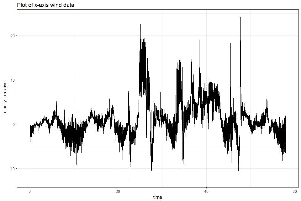
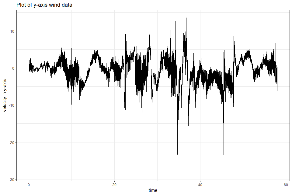
Figure 4: plot of x-axis, Met Data

Figure 5: plot of y-axis, Met Data

7 Proofs

We give the proofs of the main theorems discussed above and some preliminary ones. Some of them are also discussed in [15] with details.

We set some notations which only appear in the proof section.

1. Let us denote some $\sigma$-fields such that $\mathcal{G}_{t}:=\sigma(w_{s};s\leq t,x_{0})$, $\mathcal{G}_{j}^{n}:=\mathcal{G}_{j\Delta_{n}}$, $\mathcal{A}_{j}^{n}:=\sigma(\varepsilon_{ih_{n}};i\leq jp_{n}-1)$, $\mathcal{H}_{j}^{n}:=\mathcal{G}_{j}^{n}\vee\mathcal{A}_{j}^{n}$.

2. We define the following $\mathbf{R}^{r}$-valued random variables which appear in the expansion:

   $$\zeta_{j+1,n} =\frac{1}{p_{n}}\sum_{i=0}^{p_{n}-1}\int_{j\Delta_{n}+ih_{n}}^{(j+1)\Delta_{n}}\mathrm{d}w_{s},\ \zeta_{j+2,n}^{\prime}=\frac{1}{p_{n}}\sum_{i=0}^{p_{n}-1}\int_{(j+1)\Delta_{n}}^{(j+1)\Delta_{n}+ih_{n}}\mathrm{d}w_{s}.$$

3. $I_{j,k,n}:=I_{j,k}=[j\Delta_{n}+kh_{n},j\Delta_{n}+(k+1)h_{n}),\ j=0,\ldots,k_{n}-1,\ k=0,\ldots,p_{n}-1$.

4. We set the following empirical functionals:

   $$\bar{M}_{n}(f(\cdot,\vartheta)) :=\frac{1}{k_{n}}\sum_{j=0}^{k_{n}-1}f(\bar{Y}_{j},\vartheta),$$

   $$\bar{D}_{n}(f(\cdot,\vartheta)) :=\frac{1}{k_{n}\Delta_{n}}\sum_{j=1}^{k_{n}-2}f(\bar{Y}_{j-1},\vartheta)\left({\bar{Y}_{j+1}-\bar{Y}_{j}-\Delta_{n}b(\bar{Y}_{j-1})}\right),$$

   $$\bar{Q}_{n}(B(\cdot,\vartheta)) =\frac{1}{k_{n}\Delta_{n}}\sum_{j=1}^{k_{n}-2}B(\bar{Y}_{j-1},\vartheta)\left\llbracket\left({\bar{Y}_{j+1}-\bar{Y}_{j}}\right)^{\otimes 2}\right\rrbracket.$$

5. Let us define $D_{j,n}:=\frac{1}{2p_{n}}\sum_{i=0}^{p_{n}-1}\left({\left({Y_{j\Delta_{n}+(i+1)h_{n}}-Y_{j\Delta_{n}+ih_{n}}}\right)^{\otimes 2}-\Lambda_{\star}}\right)$, and for $1\leq l_{2}\leq l_{1}\leq d$,$D_{n}^{(l_{1},l_{2})}:=\frac{1}{k_{n}}\sum_{j=0}^{k_{n}-1}D_{j,n}^{(l_{1},l_{2})}$ and $D_{n}:=\left[D_{n}^{(1,1)},D_{n}^{(2,1)},\ldots,D_{n}^{(d,d-1)},D_{n}^{(d,d)}\right]=\mathrm{vech}\left({\hat{\Lambda}_{n}-\Lambda_{\star}}\right)$.

6. We denote

   $$\left\{B_{\kappa}\left|\kappa=1,\ldots,m_{1},\ B_{\kappa}=(B_{\kappa}^{(j_{1},j_{2})})_{j_{1},j_{2}}\right.\right\},$$

   $$\left\{f_{\lambda}\left|\lambda=1,\ldots,m_{2},\ f_{\lambda}=(f^{(1)}_{\lambda},\ldots,f^{(d)}_{\lambda})\right.\right\},$$

   which are sequences of $\mathbf{R}^{d}\otimes\mathbf{R}^{d}$-valued functions and $\mathbf{R}^{d}$-valued ones such that the components of themselves and their derivatives with respect to $x$ are polynomial growth functions for all $\kappa$ and $\lambda$.

7. Let us define

   $$\left\{B_{\kappa,n}(x)\left|\kappa=1,\ldots,m_{1},\ B_{\kappa,n}=(B_{\kappa,n}^{(j_{1},j_{2})})_{j_{1},j_{2}}\right.\right\},$$

   which is a family of sequences of the functions such that the components of the functions and their derivatives with respect to $x$ are polynomial growth functions and there exist a $\mathbf{R}$-valued sequence $\left\{{v_{n}}\right\}_{n}$ s.t. $v_{n}\to 0$ and $C>0$ such that for all $x\in\mathbf{R}^{d}$ and for the sequence $\left\{{B_{\kappa}}\right\}$ discussed above,

   $$\sum_{\kappa=1}^{m_{1}}\left\|{B_{\kappa,n}(x)-B_{\kappa}(x)}\right\|\leq v_{n}\left({1+\left\|{x}\right\|^{C}}\right).$$

8. Denote

   $$W^{(\tau)}\left({\left\{{B_{\kappa}}\right\}_{\kappa},\left\{{f_{\lambda}}\right\}_{\lambda}}\right):=\left[{\begin{matrix}W_{1}&O&O\\ O&W_{2}^{\tau}\left({\left\{{B_{\kappa}}\right\}_{\kappa}}\right)&O\\ O&O&W_{3}\left({\left\{{f_{\lambda}}\right\}_{\lambda}}\right)\end{matrix}}\right].$$

7.1 Conditional expectation of supremum

The following two propositions are multidimensional extensions of Proposition 5.1 and Proposition A in [7] respectively.

Proposition 7.

Under (A1), for all $k\geq 1$, there exists a constant $C(k)$ such that for all $t\geq 0$,

$$\mathbf{E}\left[\left.{\sup_{s\in[t,t+1]}\left\|{X_{s}}\right\|^{k}}\right|{\mathcal{G}_{t}}\right]\leq C(k)(1+\left\|{X_{t}}\right\|^{k}).$$

Proposition 8.

Under (A1) and for a function $f$ whose components are in $\mathcal{C}^{1}(\mathbf{R}^{d})$, assume that there exists $C>0$ such that

$$\left\|{f^{\prime}(x)}\right\| \leq C(1+\left\|{x}\right\|)^{C}.$$

Then for any $k\in\mathbf{N}$,

$$\mathbf{E}\left[\left.{\sup_{s\in[j\Delta_{n},(j+1)\Delta_{n}]}\left\|{f(X_{s})-f(X_{j\Delta_{n}})}\right\|^{k}}\right|{\mathcal{G}_{j}^{n}}\right]\leq C(k)\Delta_{n}^{k/2}\left({1+\left\|{X_{j\Delta_{n}}}\right\|^{C(k)}}\right).$$

Especially for $f(x)=x$,

$$\mathbf{E}\left[\left.{\sup_{s\in[j\Delta_{n},(j+1)\Delta_{n}]}\left\|{X_{s}-X_{j\Delta_{n}}}\right\|^{k}}\right|{\mathcal{G}_{j}^{n}}\right]\leq C(k)\Delta_{n}^{k/2}\left({1+\left\|{X_{j\Delta_{n}}}\right\|^{k}}\right).$$

The next proposition summarises some results useful for computation.

Proposition 9.

Under (A1), for all $t_{3}\geq t_{2}\geq t_{1}\geq 0$ where there exists a constant $C$ such that $t_{3}-t_{1}\leq C$ and $l\geq 2$, we have

$$\mathrm{(i)}\ \sup_{s_{1},s_{2}\in[t_{1},t_{2}]}\left\|{\mathbf{E}\left[\left.{b(X_{s_{1}})-b(X_{s_{2}})}\right|{\mathcal{G}_{t_{1}}}\right]}\right\|\leq C(t_{2}-t_{1})\left({1+\left\|{X_{t_{1}}}\right\|^{3}}\right),$$

$$\mathrm{(ii)}\ \sup_{s_{1},s_{2}\in[t_{1},t_{2}]}\left\|{\mathbf{E}\left[\left.{a(X_{s_{1}})-a(X_{s_{2}})}\right|{\mathcal{G}_{t_{1}}}\right]}\right\|\leq C(t_{2}-t_{1})\left({1+\left\|{X_{t_{1}}}\right\|^{3}}\right),$$

$$\mathrm{(iii)}\ \left\|{\mathbf{E}\left[\left.{\int_{t_{2}}^{t_{3}}\left({b(X_{s})-b(X_{t_{2}})}\right)\mathrm{d}s}\right|{\mathcal{G}_{t_{1}}}\right]}\right\|\leq C(t_{3}-t_{2})^{2}\left({1+\mathbf{E}\left[\left.{\left\|{X_{t_{2}}}\right\|^{6}}\right|{\mathcal{G}_{t_{1}}}\right]}\right)^{1/2},$$

$$\mathrm{(iv)}\ \mathbf{E}\left[\left.{\left\|{\int_{t_{2}}^{t_{3}}\left({b(X_{s})-b(X_{t_{2}})}\right)\mathrm{d}s}\right\|^{l}}\right|{\mathcal{G}_{t_{1}}}\right]\leq C(l)(t_{3}-t_{2})^{3l/2}\left({1+\mathbf{E}\left[\left.{\left\|{X_{t_{2}}}\right\|^{2l}}\right|{\mathcal{G}_{t_{1}}}\right]}\right),$$

$$\mathrm{(v)}\ \mathbf{E}\left[\left.{\left\|{\int_{t_{1}}^{t_{2}}\left({\int_{t_{1}}^{s}\left({a(X_{u})-a(X_{t_{1}})}\right)\mathrm{d}w_{u}}\right)\mathrm{d}s}\right\|^{l}}\right|{\mathcal{G}_{t_{1}}}\right]\leq C(l)\left({t_{2}-t_{1}}\right)^{2l}\left({1+\left\|{X_{t_{1}}}\right\|^{2l}}\right).$$

Proof.

(i), (ii): Let $L$ be the infinitesimal generator of the diffusion process. Since Ito-Taylor expansion, for all $s\in[t_{1},t_{2}]$,

$$\mathbf{E}\left[\left.{b(X_{s})}\right|{\mathcal{G}_{t_{1}}}\right]=b(X_{t_{1}})+\int_{t_{1}}^{s}\mathbf{E}\left[\left.{Lb(X_{u})}\right|{\mathcal{G}_{t_{1}}}\right]\mathrm{d}u,$$

and the second term has the evaluation

$$\sup_{s\in[t_{1},t_{2}]}\left\|{\int_{t_{1}}^{s}\mathbf{E}\left[\left.{Lb(X_{u})}\right|{\mathcal{G}_{t_{1}}}\right]\mathrm{d}u}\right\|\leq C\left(t_{2}-t_{1}\right)\left({1+\left\|{X_{t_{1}}}\right\|^{3}}\right).$$

Therefore, we have (ii) and identical revaluation holds for (ii).
(iii): Using (i) and Hölder’s inequality, we have the result.
(iv): Because of Proposition 8 and Hölder’s inequality, We obtain the proof.
(v): For convexity, we have

$$\mathbf{E}\left[\left.{\left\|{\int_{t_{1}}^{t_{2}}\left({\int_{t_{1}}^{s}\left({a(X_{u})-a(X_{t_{1}})}\right)\mathrm{d}w_{u}}\right)\mathrm{d}s}\right\|^{l}}\right|{\mathcal{G}_{t_{1}}}\right]$$

$$\leq C(l)\sum_{i=1}^{d}\sum_{j=1}^{r}\mathbf{E}\left[\left.{\left|{\int_{t_{1}}^{t_{2}}\left({\int_{t_{1}}^{s}\left({a^{(i,j)}(X_{u})-a^{(i,j)}(X_{t_{1}})}\right)\mathrm{d}w_{u}^{(j)}\mathrm{d}s}\right)^{l}}\right|}\right|{\mathcal{G}_{t_{1}}}\right].$$

Hölder’s inequality, Fubini’s theorem, BDG theorem and Proposition 8 give the result. ∎

7.2 Propositions for ergodicity and evaluations of expectation

The next result is a multivariate version of [14] or [8] using Proposition 7.

Lemma 10.

Assume (A1)-(A3) hold. Let $f$ be a function in $\mathcal{C}^{1}(\mathbf{R}^{d}\times\Xi)$ and assume that $f$, the components of $\partial_{x}f$ and $\nabla_{\vartheta}f$ are polynomial growth functions uniformly in $\vartheta\in\Xi$. Then the following convergence holds:

$$\frac{1}{k_{n}}\sum_{j=0}^{k_{n}-1}f(X_{j\Delta_{n}},\vartheta)\overset{P}{\to}\nu_{0}\left({f(\cdot,\vartheta)}\right)\ \text{uniformly in }\vartheta.$$

7.3 Characteristics of local means

The following propositions, lemmas and corollary are multidimensional extensions of those in [7] and [3].

Lemma 11.

$\zeta_{j+1,n}$ and $\zeta_{j+1,n}^{\prime}$ are $\mathcal{G}_{j+1}^{n}$-measurable, independent of $\mathcal{G}_{j}^{n}$ and Gaussian. These random variables have the following decomposition:

$$\zeta_{j+1,n} =\frac{1}{p_{n}}\sum_{k=0}^{p_{n}-1}(k_{n}+1)\int_{I_{j,k}}\mathrm{d}w_{t},$$

$$\zeta_{j+1,n}^{\prime} =\frac{1}{p_{n}}\sum_{k=0}^{p_{n}-1}(p_{n}-1-k)\int_{I_{j,k}}\mathrm{d}w_{t}.$$

In addition, the evaluation of the following conditional expectations holds:

$$\mathbf{E}\left[\left.{\zeta_{j,n}}\right|{\mathcal{G}_{j}^{n}}\right]=\mathbf{E}\left[\left.{\zeta_{j+1,n}^{\prime}}\right|{\mathcal{G}_{j}^{n}}\right] =\mathbf{0},$$

$$\mathbf{E}\left[\left.{\zeta_{j+1,n}\left({\zeta_{j+1,n}}\right)^{T}}\right|{\mathcal{G}_{j}^{n}}\right] =m_{n}\Delta_{n}I_{r},$$

$$\mathbf{E}\left[\left.{\zeta_{j+1,n}^{\prime}\left({\zeta_{j+1,n}^{\prime}}\right)^{T}}\right|{\mathcal{G}_{j}^{n}}\right] =m_{n}^{\prime}\Delta_{n}I_{r},$$

$$\mathbf{E}\left[\left.{\zeta_{j+1,n}\left({\zeta_{j+1,n}^{\prime}}\right)^{T}}\right|{\mathcal{G}_{j}^{n}}\right] =\chi_{n}\Delta_{n}I_{r},$$

where $m_{n}=\left({\frac{1}{3}+\frac{1}{2p_{n}}+\frac{1}{6p_{n}^{2}}}\right)$, $m_{n}^{\prime}=\left({\frac{1}{3}-\frac{1}{2p_{n}}+\frac{1}{6p_{n}^{2}}}\right)$ and $\chi_{n}=\frac{1}{6}\left({1-\frac{1}{p_{n}^{2}}}\right)$.

For the proof, see Lemma 8.2 in [3] and extend it to multidimensional discussion.

Proposition 12.

Under (A1), (AH), assume the component of the function $f$ on $\mathbf{R}^{d}\times\Xi$, $\partial_{x}f$ and $\partial_{x}^{2}f$ are polynomial growth functions uniformly in $\vartheta\in\Xi$. Then there exists $C>0$ such that for all $j\leq k_{n}-1$ and $\vartheta\in\Xi$,

$$\left\|{\mathbf{E}\left[\left.{f(\bar{Y}_{j}{},\vartheta)-f(X_{j\Delta_{n}},\vartheta)}\right|{\mathcal{H}_{j}^{n}}\right]}\right\|\leq C\Delta_{n}\left({1+\left\|{X_{j\Delta_{n}}}\right\|^{C}}\right).$$

Moreover, for all $l\geq 2$,

$$\mathbf{E}\left[\left.{\left\|{f(\bar{Y}_{j}{},\vartheta)-f(X_{j\Delta_{n}},\vartheta)}\right\|^{l}}\right|{\mathcal{H}_{j}^{n}}\right]\leq C(l)\Delta_{n}^{l/2}\left({1+\left\|{X_{j\Delta_{n}}}\right\|^{C(l)}}\right).$$

The proof is almost identical to that of Corollary 3.3 in [3] except for dimension, but it does not influence the evaluation.

Proposition 13.

Under (A1) and (AH),

$$\bar{Y}_{j+1}-\bar{Y}_{j}-\Delta_{n}b(\bar{Y}_{j})=a(X_{j\Delta_{n}})\left({\zeta_{j+1,n}+\zeta_{j+2,n}^{\prime}}\right)+e_{j,n}+\Lambda_{\star}^{1/2}\left({\bar{\varepsilon}_{j+1}-\bar{\varepsilon}_{j}}\right),$$

where $e_{j,n}$ is a $\mathcal{H}_{j+2}^{n}$-measurable random variable such that there exists $C>0$ and $C(l)>0$ for all $l\geq 2$ satisfying the inequalities

$$\left\|{\mathbf{E}\left[\left.{e_{j,n}}\right|{\mathcal{H}_{j}^{n}}\right]}\right\|\leq C\Delta_{n}^{2}\left({1+\left\|{X_{j\Delta_{n}}}\right\|^{5}}\right),$$

$$\mathbf{E}\left[\left.{\left\|{e_{j,n}}\right\|^{l}}\right|{\mathcal{H}_{j}^{n}}\right]\leq C(l)\Delta_{n}^{l}\left({1+\left\|{X_{j\Delta_{n}}}\right\|^{3l}}\right),$$

$$\left\|{\mathbf{E}\left[\left.{e_{j,n}\left({\zeta_{j+1,n}}\right)^{T}}\right|{\mathcal{H}_{j}^{n}}\right]}\right\|+\left\|{\mathbf{E}\left[\left.{e_{j,n}\left({\zeta_{j+2,n}^{\prime}}\right)^{T}}\right|{\mathcal{H}_{j}^{n}}\right]}\right\|\leq C\Delta_{n}^{2}\left({1+\left\|{X_{j\Delta_{n}}}\right\|^{3}}\right).$$

For the proof, see that of Proposition 3.4 in [3] and extend the discussion to multidimensional one.

Corollary 14.

Under (A1) and (AH),

$$\bar{Y}_{j+1}-\bar{Y}_{j}-\Delta_{n}b(X_{j\Delta_{n}})=a(X_{j\Delta_{n}})\left({\zeta_{j+1,n}+\zeta_{j+2,n}^{\prime}}\right)+e_{j,n}+\Lambda_{\star}^{1/2}\left({\bar{\varepsilon}_{j+1}-\bar{\varepsilon}_{j}}\right),$$

where $e_{j,n}$ is a $\mathcal{H}_{j+2}^{n}$-measurable random variable such that there exists $C>0$ and $C(l)>0$ for all $l\geq 2$ satisfying the inequalities

$$\left\|{\mathbf{E}\left[\left.{e_{j,n}}\right|{\mathcal{H}_{j}^{n}}\right]}\right\|\leq C\Delta_{n}^{2}\left({1+\left\|{X_{j\Delta_{n}}}\right\|^{5}}\right),$$

$$\mathbf{E}\left[\left.{\left\|{e_{j,n}}\right\|^{l}}\right|{\mathcal{H}_{j}^{n}}\right]\leq C(l)\Delta_{n}^{l}\left({1+\left\|{X_{j\Delta_{n}}}\right\|^{3l}}\right),$$

$$\left\|{\mathbf{E}\left[\left.{e_{j,n}\left({\zeta_{j+1,n}}\right)^{T}}\right|{\mathcal{H}_{j}^{n}}\right]}\right\|+\left\|{\mathbf{E}\left[\left.{e_{j,n}\left({\zeta_{j+2,n}^{\prime}}\right)^{T}}\right|{\mathcal{H}_{j}^{n}}\right]}\right\|\leq C\Delta_{n}^{2}\left({1+\left\|{X_{j\Delta_{n}}}\right\|^{3}}\right).$$

Proof.

It is enough to see $\Delta_{n}b(\bar{Y}_{j})-\Delta_{n}b(X_{j\Delta_{n}})$ satisfies the evaluation for $e_{j,n}$. Corollary 12 and Proposition 13 give

$$\left\|{\mathbf{E}\left[\left.{\Delta_{n}b(\bar{Y}_{j})-\Delta_{n}b(X_{j\Delta_{n}})}\right|{\mathcal{H}_{j}^{n}}\right]}\right\|\leq C\Delta_{n}^{2}\left({1+\left\|{X_{j\Delta_{n}}}\right\|^{5}}\right),$$

$$\mathbf{E}\left[\left.{\left\|{\Delta_{n}b(\bar{Y}_{j})-\Delta_{n}b(X_{j\Delta_{n}})}\right\|^{l}}\right|{\mathcal{H}_{j}^{n}}\right]\leq C(l)\Delta_{n}^{l}\left({1+\left\|{X_{j\Delta_{n}}}\right\|^{3l}}\right).$$

With respect to the third evaluation, Hölder’s inequality verifies the result. ∎

The following lemma summarises some useful evaluations for computation.

Lemma 15.

Assume $f$ is a function whose components are in $\mathcal{C}^{2}(\mathbf{R}^{d}\times\Xi)$ and the components of $f$ and $\partial_{x}f$ are polynomial growth functions in $\vartheta\in\Xi$. In addition, $g$ denotes a function whose components are in $\mathcal{C}^{2}(\mathbf{R}^{d})$ and that the components of $g$ and $\partial_{x}g$ are polynomial growth functions. Under (A1), (A3), (A4) and (AH), the following uniform evaluation holds:

$$\mathrm{(i)} {}^{\forall}l_{1},l_{2}\in\mathbf{N}_{0},\ \sup_{j,n}\mathbf{E}\left[{\sup_{\vartheta\in\Xi}\left\|{f(\bar{Y}_{j-1},\vartheta)}\right\|^{l_{1}}\left({1+\left\|{X_{j\Delta_{n}}}\right\|}\right)^{l_{2}}}\right]\leq C(l_{1},l_{2}),$$

$$\mathrm{(ii)} {}^{\forall}l\in\mathbf{N},\ ^{\forall}j\leq k_{n}-2,\ \mathbf{E}\left[{\left\|{\zeta_{j+1,n}+\zeta_{j+2,n}^{\prime}}\right\|^{l}}\right]\leq C(l)\Delta_{n}^{l/2},$$

$$\mathrm{(iii)} {}^{\forall}l\in\mathbf{N},\ ^{\forall}j\leq k_{n}-1,\ \mathbf{E}\left[{\left\|{g(X_{(j+1)\Delta_{n}})-g(X_{j\Delta_{n}})}\right\|^{l}}\right]\leq C(l)\Delta_{n}^{l/2},$$

$$\mathrm{(iv)} {}^{\forall}l\in\mathbf{N},\ ^{\forall}j\leq k_{n}-1,\ \mathbf{E}\left[{\left\|{g(\bar{Y}_{j})-g(X_{j\Delta_{n}})}\right\|^{l}}\right]\leq C(l)\Delta_{n}^{l/2},$$

$$\mathrm{(v)} {}^{\forall}l\in\mathbf{N},\ ^{\forall}j\leq k_{n}-2,\ \mathbf{E}\left[{\left\|{g(\bar{Y}_{j+1})-g(\bar{Y}_{j})}\right\|^{l}}\right]\leq C(l)\Delta_{n}^{l/2},$$

$$\mathrm{(vi)} {}^{\forall}l\in\mathbf{N},\ ^{\forall}j\leq k_{n}-2,\ \mathbf{E}\left[{\left\|{e_{j,n}}\right\|^{l}}\right]\leq C(l)\Delta_{n}^{l},$$

$$\mathrm{(vii)} {}^{\forall}l\in\mathbf{N},\ \sup_{j,n}\left({\frac{\mathbf{E}\left[\left\|{\bar{\varepsilon}_{j}}\right\|^{l}\right]}{\Delta_{n}^{l/2}}}\right)\leq C(l).$$

Proof.

Simple computations and the results above lead to the proof. ∎

7.4 Uniform law of large numbers

The following propositions and theorems are multidimensional version of [3].

Proposition 16.

Assume $f$ is a function in $\mathcal{C}^{2}(\mathbf{R}^{d}\times\Xi)$ and $f$, the components of $\partial_{x}f$, $\partial_{x}^{2}f$ and $\partial_{\vartheta}f$ are polynomial growth functions uniformly in $\vartheta\in\Xi$. Under (A1)-(A4), (AH),

$$\bar{M}_{n}(f(\cdot,\vartheta))\overset{P}{\to}\nu_{0}(f(\cdot,\vartheta))\text{ uniformly in }\vartheta.$$

The proof is almost same as Proposition 4.1 in [3].

Theorem 17.

Assume $f=\left({f^{1},\ldots,f^{d}}\right)$ is a function in $\mathcal{C}^{2}(\mathbf{R}^{d}\times\Xi;\mathbf{R}^{d})$ and the components of $f$, $\partial_{x}f$, $\partial_{x}^{2}f$ and $\partial_{\vartheta}f$ are polynomial growth functions uniformly in $\vartheta\in\Xi$. Under (A1)-(A4), (AH),

$$\bar{D}_{n}(f(\cdot,\vartheta))\overset{P}{\to}0\text{ uniformly in }\vartheta.$$

Proof.

We define the following random variables:

$$V_{j}^{n}(\vartheta) :=f(\bar{Y}_{j-1},\vartheta)\left({\bar{Y}_{j+1}-\bar{Y}_{j}-\Delta_{n}b(\bar{Y}_{j})}\right),$$

$$\tilde{D}_{n}(f(\cdot,\vartheta)) :=\frac{1}{k_{n}\Delta_{n}}\sum_{j=1}^{k_{n}-2}V_{j}^{n}(\vartheta)$$

and then

$$\bar{D}_{n}(f(\cdot,\vartheta)) =\tilde{D}_{n}(\cdot,\vartheta)+\frac{1}{k_{n}}\sum_{j=1}^{k_{n}-2}f(\bar{Y}_{j-1},\vartheta)\left({b(\bar{Y}_{j})-b(\bar{Y}_{j-1})}\right).$$

Hence it is enough to see the uniform convergences in probability of the first term and the second one in the right hand side.

In the first place, we consider the first term of the right hand side above. We can decompose the sum of $V_{j}^{n}(\vartheta)$ as follows:

$$\sum_{j=1}^{k_{n}-2}V_{j}^{n}(\vartheta)=\sum_{1\leq 3j\leq k_{n}-2}V_{3j}^{n}(\vartheta)+\sum_{1\leq 3j+1\leq k_{n}-2}V_{3j+1}^{n}(\vartheta)+\sum_{1\leq 3j+2\leq k_{n}-2}V_{3j+2}^{n}(\vartheta).$$

To simplify notations, we only consider the first term of the right hand side and the other terms have the identical evaluation. Let us define the following random variables:

$$v_{3j,n}^{(1)}(\vartheta) :=f(\bar{Y}_{3j-1},\vartheta)a(X_{3j\Delta_{n}})\left({\zeta_{3j+1,n}+\zeta_{3j+2,n}^{\prime}}\right),$$

$$v_{3j,n}^{(2)}(\vartheta) :=f(\bar{Y}_{3j-1},\vartheta)\Lambda_{\star}^{1/2}\left({\bar{\varepsilon}_{3j+1}-\bar{\varepsilon}_{3j}}\right),$$

$$v_{3j,n}^{(3)}(\vartheta) :=f(\bar{Y}_{3j-1},\vartheta)e_{3j,n},$$

and recall Proposition 13 which states

$$\bar{Y}_{j+1}-\bar{Y}_{j}-\Delta_{n}b(\bar{Y}_{j})=a(X_{j\Delta_{n}})\left({\zeta_{j+1,n}+\zeta_{j+2,n}^{\prime}}\right)+e_{j,n}+\Lambda_{\star}^{1/2}\left({\bar{\varepsilon}_{j+1}-\bar{\varepsilon}_{j}}\right).$$

Therefore we have

$$V_{3j}^{n}(\vartheta)=v_{3j,n}^{(1)}(\vartheta)+v_{3j,n}^{(2)}(\vartheta)+v_{3j,n}^{(3)}(\vartheta).$$

First of all, the pointwise convergence to 0 for all $\vartheta$ and we abbreviate $f(\cdot,\vartheta)$ as $f(\cdot)$. Since $V_{3j}^{n}$ is $\mathcal{H}_{3j+2}^{n}$-measurable and hence $\mathcal{H}_{3j+3}^{n}$-measurable, the sequence of random variables $\left\{{V_{3j}}\right\}_{1\leq 3j\leq k_{n}-2}$ are $\left\{{\mathcal{H}_{3j+3}^{n}}\right\}_{1\leq 3j\leq k_{n}-2}$-adopted, and hence it is enough to see

$$\frac{1}{k_{n}\Delta_{n}}\sum_{1\leq 3j\leq k_{n}-2}\mathbf{E}\left[\left.{V_{3j}^{n}}\right|{\mathcal{H}_{3(j-1)+3}^{n}}\right]=\frac{1}{k_{n}\Delta_{n}}\sum_{1\leq 3j\leq k_{n}-2}\mathbf{E}\left[\left.{V_{3j}^{n}}\right|{\mathcal{H}_{3j}^{n}}\right] \overset{P}{\to}0,$$

$$\frac{1}{k_{n}^{2}\Delta_{n}^{2}}\sum_{1\leq 3j\leq k_{n}-2}\mathbf{E}\left[\left.{\left({V_{3j}^{n}}\right)^{2}}\right|{\mathcal{H}_{3j}^{n}}\right] \overset{P}{\to}0$$

because of Lemma 9 in [6]. It is quite routine to show it because of Proposition 13.

Next, we consider the uniform convergence in probability of $\tilde{D}_{n}(f(\cdot,\vartheta))$. Let us define

$$S_{n}^{(l)}(\vartheta):=\frac{1}{k_{n}\Delta_{n}}\sum_{1\leq 3j\leq k_{n}-2}v_{3j,n}^{(l)}(\vartheta),\ l=1,2,3.$$

We will see for all $l$, $S_{n}^{(l)}(\vartheta)$ uniformly converges to 0 in probability. Firstly we examine $S_{n}^{(3)}$: Lemma 15 gives

$$\mathbf{E}\left[{\sup_{\vartheta\in\Xi}\left|{\nabla_{\vartheta}v_{3j,n}^{(3)}(\vartheta)}\right|}\right]\leq C\Delta_{n}.$$

Hence we obtain

$$\sup_{n\in\mathbf{N}}\mathbf{E}\left[{\sup_{\vartheta\in\Xi}\left|{\nabla_{\vartheta}S_{n}^{(3)}(\vartheta)}\right|}\right]\leq C<\infty.$$

Therefore it holds

$$S_{n}^{(3)}(\vartheta)\overset{P}{\to}0\text{ uniformly in }\vartheta$$

as the discussion in [14] or Proposition A1 in [8].

For $S_{n}^{(l)},\ l=1,2$ we see the following inequalities hold (see [11]): there exist $C>0$ and $\kappa>\dim\Xi$ such that

$$\mathrm{(1)} {}^{\forall}\vartheta\in\Xi,\ ^{\forall}n\in\mathbf{N},\ \mathbf{E}\left[{\left|{S_{n}^{(l)}(\vartheta)}\right|^{\kappa}}\right]\leq C,$$

$$\mathrm{(2)} {}^{\forall}\vartheta,\vartheta^{\prime}\in\Xi,\ ^{\forall}n\in\mathbf{N},\ \mathbf{E}\left[{\left|{S_{n}^{(l)}(\vartheta)-S_{n}^{(l)}(\vartheta^{\prime})}\right|^{\kappa}}\right]\leq C\left\|{\vartheta-\vartheta^{\prime}}\right\|^{\kappa}.$$

Assume $\kappa=2k,\ k\in\mathbf{N}$ in the following discussion.

For $l=1$, Burkholder’s inequality and Lemma 15gives that for all $\kappa$, there exists $C=C(\kappa)$ such that

$$\mathbf{E}\left[{\left|{S_{n}^{(1)}(\vartheta)}\right|^{\kappa}}\right] \leq\frac{C(\kappa)}{\left({k_{n}\Delta_{n}}\right)^{\kappa}}k_{n}^{\kappa/2-1}\sum_{1\leq 3j\leq k_{n}-2}\mathbf{E}\left[{\left|{v_{3j,n}^{(1)}(\vartheta)}\right|^{\kappa}}\right]$$

$$\leq\frac{C(\kappa)}{\left({k_{n}\Delta_{n}}\right)^{\kappa}}k_{n}^{\kappa/2-1}\sum_{1\leq 3j\leq k_{n}-2}C(\kappa)\Delta_{n}^{\kappa/2}$$

$$\leq\frac{C(\kappa)}{\left({k_{n}\Delta_{n}}\right)^{\kappa/2}}.$$

With respect to $\mathbf{E}\left[{\left|{S_{n}^{(1)}(\vartheta)-S_{n}^{(1)}(\vartheta^{\prime})}\right|^{\kappa}}\right]$, identically

$$\mathbf{E}\left[{\left|{S_{n}^{(1)}(\vartheta)-S_{n}^{(1)}(\vartheta^{\prime})}\right|^{\kappa}}\right] \leq\frac{C(\kappa)}{\left({k_{n}\Delta_{n}}\right)^{\kappa}}k_{n}^{\kappa/2-1}\sum_{1\leq 3j\leq k_{n}-2}\mathbf{E}\left[{\left|{v_{3j,n}^{(1)}(\vartheta)-v_{3j,n}^{(1)}(\vartheta^{\prime})}\right|^{\kappa}}\right]$$

$$\leq\frac{C(\kappa)}{\left({k_{n}\Delta_{n}}\right)^{\kappa}}k_{n}^{\kappa/2-1}\sum_{1\leq 3j\leq k_{n}-2}C(\kappa)\Delta_{n}^{\kappa/2}\left\|{\vartheta-\vartheta^{\prime}}\right\|^{\kappa}$$

$$\leq\frac{C(\kappa)}{\left({k_{n}\Delta_{n}}\right)^{\kappa/2}}\left\|{\vartheta-\vartheta^{\prime}}\right\|^{\kappa}.$$

This result gives uniform convergence in probability of $S_{n}^{(1)}$. The identical evaluation holds for $S_{n}^{(2)}$ and then these lead to uniform convergence of $\tilde{D}_{n}\left({\vartheta}\right)$.

Finally we check the uniform convergence in probability of the following random variable,

$$\frac{1}{k_{n}}\sum_{1\leq 3j\leq k_{n}-2}f(\bar{Y}_{j-1},\vartheta)\left({b(\bar{Y}_{j})-b(\bar{Y}_{j-1})}\right).$$

By Lemma 15, it is easily shown that

$$\mathbf{E}\left[{\sup_{\vartheta\in\Xi}\left|{\frac{1}{k_{n}}\sum_{1\leq 3j\leq k_{n}-2}f(\bar{Y}_{j-1},\vartheta)\left({b(\bar{Y}_{j})-b(\bar{Y}_{j-1})}\right)}\right|}\right]\to 0.$$

It completes the proof. ∎

Theorem 18.

Assume $B=\left({B^{\left(i,j\right)}}\right)_{i,j}$ is a function in $\mathcal{C}^{2}(\mathbf{R}^{d}\times\Xi;\mathbf{R}^{d}\otimes\mathbf{R}^{d})$ and the components of $B$, $\partial_{x}B$, $\partial_{x}^{2}B$ and $\partial_{\vartheta}B$ are polynomial growth functions uniformly in $\vartheta\in\Xi$. Under (A1)-(A4), (AH), if $\tau\in(1,2]$,

$$\bar{Q}_{n}(B(\cdot,\vartheta))\overset{P}{\to}\frac{2}{3}\nu_{0}\left({B(\cdot,\vartheta)\left\llbracket A^{\tau}(\cdot,\alpha^{\star},\Lambda_{\star})\right\rrbracket}\right)\text{ uniformly in }\vartheta.$$

Proof.

We define $q_{j,n}(\vartheta):=\sum_{i=1}^{6}q_{j,n}^{(i)}(\vartheta)$ where

$$q_{j,n}^{(1)}(\vartheta) :=B(\bar{Y}_{j-1},\vartheta)\left\llbracket\left({a(X_{j\Delta_{n}})\left({\zeta_{j+1,n}+\zeta_{j+2,n}^{\prime}}\right)}\right)^{\otimes 2}\right\rrbracket,$$

$$q_{j,n}^{(2)}(\vartheta) :=B(\bar{Y}_{j-1},\vartheta)\left\llbracket\left({\Lambda_{\star}^{1/2}\left({\bar{\varepsilon}_{j+1}-\bar{\varepsilon}_{j}}\right)}\right)^{\otimes 2}\right\rrbracket,$$

$$q_{j,n}^{(3)}(\vartheta) :=B(\bar{Y}_{j-1},\vartheta)\left\llbracket\left({\Delta_{n}b(\bar{Y}_{j})+e_{j,n}}\right)^{\otimes 2}\right\rrbracket,$$

$$q_{j,n}^{(4)}(\vartheta) :=B(\bar{Y}_{j-1},\vartheta)\left\llbracket a(X_{j\Delta_{n}})\left({\zeta_{j+1,n}+\zeta_{j+2,n}^{\prime}}\right)\left({\Lambda_{\star}^{1/2}\left({\bar{\varepsilon}_{j+1}-\bar{\varepsilon}_{j}}\right)}\right)^{T}\right\rrbracket,$$

$$\qquad+B(\bar{Y}_{j-1},\vartheta)\left\llbracket\left({\Lambda_{\star}^{1/2}\left({\bar{\varepsilon}_{j+1}-\bar{\varepsilon}_{j}}\right)}\right)\left({\zeta_{j+1,n}+\zeta_{j+2,n}^{\prime}}\right)^{T}a(X_{j\Delta_{n}})^{T}\right\rrbracket,$$

$$q_{j,n}^{(5)}(\vartheta) :=B(\bar{Y}_{j-1},\vartheta)\left\llbracket a(X_{j\Delta_{n}})\left({\zeta_{j+1,n}+\zeta_{j+2,n}^{\prime}}\right)\left({\Delta_{n}b(\bar{Y}_{j})+e_{j,n}}\right)^{T}\right\rrbracket$$

$$\qquad+B(\bar{Y}_{j-1},\vartheta)\left\llbracket\left({\Delta_{n}b(\bar{Y}_{j})+e_{j,n}}\right)\left({\zeta_{j+1,n}+\zeta_{j+2,n}^{\prime}}\right)^{T}a(X_{j\Delta_{n}})^{T}\right\rrbracket,$$

$$q_{j,n}^{(6)}(\vartheta) :=B(\bar{Y}_{j-1},\vartheta)\left\llbracket\left({\Delta_{n}b(\bar{Y}_{j})+e_{j,n}}\right)\left({\Lambda_{\star}^{1/2}\left({\bar{\varepsilon}_{j+1}-\bar{\varepsilon}_{j}}\right)}\right)^{T}\right\rrbracket,$$

$$\qquad+B(\bar{Y}_{j-1},\vartheta)\left\llbracket\left({\Lambda_{\star}^{1/2}\left({\bar{\varepsilon}_{j+1}-\bar{\varepsilon}_{j}}\right)}\right)\left({\Delta_{n}b(\bar{Y}_{j})+e_{j,n}}\right)^{T}\right\rrbracket,$$

and then for Proposition 13 we obtain

$$\bar{Q}_{n}(B(\cdot,\vartheta))=\frac{1}{k_{n}\Delta_{n}}\sum_{j=1}^{k_{n}-2}q_{j,n}(\vartheta).$$

We examine the following quantities which divide the summation into three parts: for $l=0,1,2$,

$$T_{l,n}^{(i)}(\vartheta):=\frac{1}{k_{n}\Delta_{n}}\sum_{1\leq 3j+l\leq k_{n}-2}q_{3j+l,n}^{(i)}(\vartheta)\text{ for }i=1,\ldots,6.$$

Firstly we see the pointwise-convergence in probability with respect to $\vartheta$.

We examine $T_{0,n}^{(1)}(\vartheta)$ and consider to show convergence in probability with Lemma 9 in [6]. Lemma 11 gives

$$\mathbf{E}\left[\left.{q_{3j,n}^{(1)}(\vartheta)}\right|{\mathcal{H}_{3j}^{n}}\right]=\left({\frac{2}{3}+\frac{1}{3p_{n}^{2}}}\right)\Delta_{n}B(\bar{Y}_{3j-1},\vartheta)\left\llbracket A(X_{3j\Delta_{n}})\right\rrbracket.$$

Note that Lemma 10 gives

$$\frac{1}{k_{n}\Delta_{n}}\sum_{1\leq 3j\leq k_{n}-2}\left({\frac{2}{3}+\frac{1}{3p_{n}^{2}}}\right)\Delta_{n}B(X_{3j\Delta_{n}},\vartheta)\left\llbracket A(X_{3j\Delta_{n}})\right\rrbracket\overset{P}{\to}\frac{1}{3}\times\frac{2}{3}\times\nu_{0}\left({B(\cdot,\vartheta)\left\llbracket A(\cdot)\right\rrbracket}\right),$$

and we can obtain

$$\frac{1}{k_{n}}\sum_{1\leq 3j\leq k_{n}-2}\left({\frac{2}{3}+\frac{1}{3p_{n}^{2}}}\right)\left({B(X_{3j\Delta_{n}},\vartheta)-B(X_{(3j-1)\Delta_{n}},\vartheta)}\right)\left\llbracket A(X_{3j\Delta_{n}})\right\rrbracket \overset{P}{\to}0$$

$$\frac{1}{k_{n}}\sum_{1\leq 3j\leq k_{n}-2}\left({\frac{2}{3}+\frac{1}{3p_{n}^{2}}}\right)\left({B(\bar{Y}_{3j-1},\vartheta)-B(X_{(3j-1)\Delta_{n}},\vartheta)}\right)\left\llbracket A(X_{3j\Delta_{n}})\right\rrbracket \overset{P}{\to}0$$

because of Lemma 15; hence we have

$$\frac{1}{k_{n}\Delta_{n}}\sum_{1\leq 3j\leq k_{n}-2}\mathbf{E}\left[\left.{q_{3j,n}^{(1)}(\vartheta)}\right|{\mathcal{H}_{3j}^{n}}\right]\overset{P}{\to}\frac{2}{9}\nu_{0}\left({B(\cdot,\vartheta)\left\llbracket A(\cdot)\right\rrbracket}\right).$$

Next we have

$$\mathbf{E}\left[\left.{\left|{q_{3j,n}^{(1)}(\vartheta)}\right|^{2}}\right|{\mathcal{H}_{3j}^{n}}\right]\leq C\Delta_{n}^{2}\left\|{B(\bar{Y}_{3j-1},\vartheta)}\right\|^{2}\left\|{a(X_{3j\Delta_{n}})}\right\|^{4}$$

because of Lemma 15, and then we obtain

$$\mathbf{E}\left[{\left|{\frac{1}{k_{n}^{2}\Delta_{n}^{2}}\sum_{1\leq 3j\leq k_{n}-2}\mathbf{E}\left[\left.{\left|{q_{3j,n}^{(1)}(\vartheta)}\right|^{2}}\right|{\mathcal{H}_{3j}^{n}}\right]}\right|}\right]\to 0$$

also because of Lemma 15. Therefore, Lemma 9 in [6] gives

$$T_{0,n}^{(1)}(\vartheta)\overset{P}{\to}\frac{2}{9}\nu_{0}\left({B(\cdot,\vartheta)\left\llbracket A(\cdot)\right\rrbracket}\right)$$

and identical convergences for $T_{1,n}^{(1)}(\vartheta)$ and $T_{2,n}^{(1)}(\vartheta)$ can be given. Hence

$$T_{0,n}^{(1)}(\vartheta)+T_{1,n}^{(1)}(\vartheta)+T_{2,n}^{(1)}(\vartheta)\overset{P}{\to}\frac{2}{3}\nu_{0}\left({B(\cdot,\vartheta)\left\llbracket A(\cdot)\right\rrbracket}\right).$$

For $T_{0,n}^{(2)}(\vartheta)$, we also see the pointwise convergence in probability with [6]. Firstly,

$$\mathbf{E}\left[\left.{q_{3j,n}^{(2)}(\vartheta)}\right|{\mathcal{H}_{3j}^{n}}\right]=\frac{2}{p_{n}}B(\bar{Y}_{j-1},\vartheta)\left\llbracket\Lambda_{\star}\right\rrbracket$$

and then Proposition 16 leads to

$$\frac{1}{k_{n}\Delta_{n}}\sum_{1\leq 3j\leq k_{n}-2}\mathbf{E}\left[\left.{q_{3j,n}^{(2)}(\vartheta)}\right|{\mathcal{H}_{3j}^{n}}\right]\overset{P}{\to}\begin{cases}0&\text{ if }\tau\in(1,2)\\ \frac{2}{3}\nu_{0}\left({B(\cdot,\vartheta)\left\llbracket\Lambda_{\star}\right\rrbracket}\right)&\text{ if }\tau=2\end{cases}$$

because

$$\frac{1}{p_{n}\Delta_{n}}=\frac{1}{p_{n}^{2}h_{n}}=\frac{1}{p_{n}^{2-\tau}}\to\begin{cases}0&\text{ if }\tau\in(1,2)\\ 1&\text{ if }\tau=2.\end{cases}$$

Because of Lemma 15, we also easily have the conditional second moment evaluation such that

$$\mathbf{E}\left[{\left|{\frac{1}{k_{n}^{2}\Delta_{n}^{2}}\sum_{1\leq 3j\leq k_{n}-2}\mathbf{E}\left[\left.{\left|{q_{3j,n}^{(2)}(\vartheta)}\right|^{2}}\right|{\mathcal{H}_{3j}^{n}}\right]}\right|}\right]\to 0,$$

therefore this $L^{1}$ convergence verifies convergence in probability and by Lemma 9 in [6],

$$T_{0,n}^{(2)}(\vartheta)\overset{P}{\to}\begin{cases}0&\text{ if }\tau\in(1,2)\\ \frac{2}{3}\nu_{0}\left({B(\cdot,\vartheta)\left\llbracket\Lambda_{\star}\right\rrbracket}\right)&\text{ if }\tau=2\end{cases}$$

and then

$$T_{0,n}^{(2)}(\vartheta)+T_{1,n}^{(2)}(\vartheta)+T_{2,n}^{(2)}(\vartheta)\overset{P}{\to}\begin{cases}0&\text{ if }\tau\in(1,2)\\ 2\nu_{0}\left({B(\cdot,\vartheta)\left\llbracket\Lambda_{\star}\right\rrbracket}\right)&\text{ if }\tau=2.\end{cases}$$

It is easy to show $T_{0,n}^{(l)}(\vartheta)\overset{P}{\to}0$ for $l=3,\ldots,6$. Here we have pointwise convergence in probability of $\bar{Q}_{n}(B(\cdot,\vartheta))$ for all $\vartheta$.

Finally we see the uniform convergence. It can be obtained as

$$\sup_{n\in\mathbf{N}}\mathbf{E}\left[{\sup_{\vartheta\in\Xi}\left|{\nabla\bar{Q}_{n}(B(\cdot,\vartheta))}\right|}\right]\leq C$$

whose computation is verified by Lemma 15. Therefore uniform convergence in probability is obtained. ∎

7.5 Asymptotic normality

Theorem 19.

Under (A1)-(A5), (AH) and $k_{n}\Delta_{n}^{2}\to 0$,

$$\left[{\begin{matrix}\sqrt{n}D_{n}\\ \sqrt{k_{n}}\left[{\bar{Q}_{n}\left({B_{\kappa}(\cdot)}\right)-\frac{2}{3}\bar{M}_{n}\left({B_{\kappa}(\cdot)\left\llbracket A_{n}^{\tau}\left({\cdot,\alpha^{\star},\Lambda_{\star}}\right)\right\rrbracket}\right)}\right]_{\kappa}\\ \sqrt{k_{n}\Delta_{n}}\left[{\bar{D}_{n}\left({f_{\lambda}(\cdot)}\right)}\right]^{\lambda}\end{matrix}}\right]\overset{\mathcal{L}}{\to}N(\mathbf{0},W^{(\tau)}(\left\{{B_{\kappa}}\right\},\left\{{f_{\lambda}}\right\})),$$

where

$$A_{n}^{\tau}(x,\alpha,\Lambda) :=A(x,\alpha)+3\Delta_{n}^{\frac{2-\tau}{\tau-1}}\Lambda.$$

Proof.

(Step 1): We can decompose

$$\sqrt{n}\left({\hat{\Lambda}_{n}-\Lambda_{\star}}\right) =\frac{1}{2\sqrt{n}}\sum_{i=0}^{n-1}\left({X_{(i+1)h_{n}}-X_{ih_{n}}}\right)^{\otimes 2}$$

$$\qquad+\frac{1}{2\sqrt{n}}\sum_{i=0}^{n-1}\Lambda_{\star}^{1/2}\left({\left({\varepsilon_{(i+1)h_{n}}-\varepsilon_{ih_{n}}}\right)^{\otimes 2}-I_{d}}\right)\Lambda_{\star}^{1/2}$$

$$\qquad+\frac{1}{2\sqrt{n}}\sum_{i=0}^{n-1}\left({X_{(i+1)h_{n}}-X_{ih_{n}}}\right)\left({\varepsilon_{(i+1)h_{n}}-\varepsilon_{ih_{n}}}\right)^{T}\Lambda_{\star}^{1/2}$$

$$\qquad+\frac{1}{2\sqrt{n}}\sum_{i=0}^{n-1}\Lambda_{\star}^{1/2}\left({\varepsilon_{(i+1)h_{n}}-\varepsilon_{ih_{n}}}\right)\left({X_{(i+1)h_{n}}-X_{ih_{n}}}\right)^{T}.$$

The first, third and fourth terms in right hand side are $o_{P}(1)$ which can be shown by $L^{1}$-evaluation and Lemma 9 in [6]. Then we obtain

$$\sqrt{n}\left({\hat{\Lambda}_{n}-\Lambda_{\star}}\right) =\frac{1}{2\sqrt{n}}\sum_{i=0}^{n-1}\Lambda_{\star}^{1/2}\left({\left({\varepsilon_{(i+1)h_{n}}-\varepsilon_{ih_{n}}}\right)^{\otimes 2}-2I_{d}}\right)\Lambda_{\star}^{1/2}+o_{P}(1)$$

and

$$\sqrt{n}D_{n} =\frac{1}{2\sqrt{n}}\sum_{i=0}^{n-1}\mathrm{vech}\left({\Lambda_{\star}^{1/2}\left({\left({\varepsilon_{(i+1)h_{n}}-\varepsilon_{ih_{n}}}\right)^{\otimes 2}-2I_{d}}\right)\Lambda_{\star}^{1/2}}\right)+o_{P}(1).$$

We can rewrite the summation as

$$\frac{1}{2\sqrt{n}}\sum_{i=0}^{n-1}\Lambda_{\star}^{1/2}\left({\left({\varepsilon_{(i+1)h_{n}}-\varepsilon_{ih_{n}}}\right)^{\otimes 2}-2I_{d}}\right)\Lambda_{\star}^{1/2}$$

$$=\frac{1}{2\sqrt{n}}\sum_{i=1}^{n-1}\Lambda_{\star}^{1/2}\left({2\left({\varepsilon_{ih_{n}}}\right)^{\otimes 2}+\left({\varepsilon_{ih_{n}}}\right)\left({\varepsilon_{(i-1)h_{n}}}\right)^{T}+\left({\varepsilon_{(i-1)h_{n}}}\right)\left({\varepsilon_{ih_{n}}}\right)^{T}-2I_{d}}\right)\Lambda_{\star}^{1/2}+o_{P}(1)$$

$$=\frac{1}{2\sqrt{n}}\sum_{i=p_{n}}^{n-p_{n}-1}\Lambda_{\star}^{1/2}\left({2\left({\varepsilon_{ih_{n}}}\right)^{\otimes 2}+\left({\varepsilon_{ih_{n}}}\right)\left({\varepsilon_{(i-1)h_{n}}}\right)^{T}+\left({\varepsilon_{(i-1)h_{n}}}\right)\left({\varepsilon_{ih_{n}}}\right)^{T}-2I_{d}}\right)\Lambda_{\star}^{1/2}$$

$$\qquad+o_{P}(1)$$

where the last evaluation holds because of Lemma 9 in [6], and then

$$\sqrt{n}D_{n} =\frac{\sqrt{n}}{k_{n}}\sum_{j=1}^{k_{n}-2}D_{j,n}^{\prime}+o_{P}(1),$$

where

$$D_{j,n}^{\prime} =\frac{1}{2p_{n}}\sum_{i=0}^{p_{n}-1}\mathrm{vech}\left({\Lambda_{\star}^{1/2}\left({2\left({\varepsilon_{j\Delta_{n}+ih_{n}}}\right)^{\otimes 2}+\left({\varepsilon_{j\Delta_{n}+ih_{n}}}\right)\left({\varepsilon_{j\Delta_{n}+(i-1)h_{n}}}\right)^{T}}\right.}\right.$$

$$\qquad\qquad\qquad\qquad\qquad\left.{\left.{+\left({\varepsilon_{j\Delta_{n}+(i-1)h_{n}}}\right)\left({\varepsilon_{j\Delta_{n}+ih_{n}}}\right)^{T}-2I_{d}}\right)\Lambda_{\star}^{1/2}}\right),$$

$$\left({D_{j,n}^{\prime}}\right)^{(l_{1},l_{2})} =\frac{1}{2p_{n}}\sum_{i=0}^{p_{n}-1}\left({\Lambda_{\star}^{1/2}\left({2\left({\varepsilon_{j\Delta_{n}+ih_{n}}}\right)^{\otimes 2}+\left({\varepsilon_{j\Delta_{n}+ih_{n}}}\right)\left({\varepsilon_{j\Delta_{n}+(i-1)h_{n}}}\right)^{T}}\right.}\right.$$

$$\qquad\qquad\qquad\qquad\qquad\left.{\left.{+\left({\varepsilon_{j\Delta_{n}+(i-1)h_{n}}}\right)\left({\varepsilon_{j\Delta_{n}+ih_{n}}}\right)^{T}-2I_{d}}\right)\Lambda_{\star}^{1/2}}\right)^{(l_{1},l_{2})}.$$

The conditional moment of $u_{i}$ is given as

$$\mathbf{E}\left[\left.{D_{j,n}^{\prime}}\right|{\mathcal{H}_{j}^{n}}\right]=\mathbf{0}.$$

Note that

$$\left({\Lambda_{\star}^{1/2}\left({2\left({\varepsilon_{ih_{n}}}\right)^{\otimes 2}+\left({\varepsilon_{ih_{n}}}\right)\left({\varepsilon_{(i-1)h_{n}}}\right)^{T}+\left({\varepsilon_{(i-1)h_{n}}}\right)\left({\varepsilon_{ih_{n}}}\right)^{T}-2I_{d}}\right)\Lambda_{\star}^{1/2}}\right)^{(l_{1},l_{2})}$$

$$=2\left({\sum_{k_{1}=1}^{d}\left({\Lambda_{\star}^{1/2}}\right)^{(l_{1},k_{1})}\left({\varepsilon_{ih_{n}}^{(k_{1})}}\right)}\right)\left({\sum_{k_{2}=1}^{d}\left({\varepsilon_{ih_{n}}^{(k_{2})}}\right)\left({\Lambda_{\star}^{1/2}}\right)^{(k_{2},l_{2})}}\right)$$

$$\qquad+\left({\sum_{k_{1}=1}^{d}\left({\Lambda_{\star}^{1/2}}\right)^{(l_{1},k_{1})}\left({\varepsilon_{ih_{n}}^{(k_{1})}}\right)}\right)\left({\sum_{k_{2}=1}^{d}\left({\varepsilon_{(i-1)h_{n}}^{(k_{2})}}\right)\left({\Lambda_{\star}^{1/2}}\right)^{(k_{2},l_{2})}}\right)$$

$$\qquad+\left({\sum_{k_{1}=1}^{d}\left({\Lambda_{\star}^{1/2}}\right)^{(l_{1},k_{1})}\left({\varepsilon_{(i-1)h_{n}}^{(k_{1})}}\right)}\right)\left({\sum_{k_{2}=1}^{d}\left({\varepsilon_{ih_{n}}^{(k_{2})}}\right)\left({\Lambda_{\star}^{1/2}}\right)^{(k_{2},l_{2})}}\right)$$

$$\qquad-2\Lambda_{\star}^{(l_{1},l_{2})}$$

and hence

$$\tilde{D}_{ih_{n},n}\left({(l_{1},l_{2}),(l_{3},l_{4})}\right)$$

$$:=\mathbf{E}\left[{\left({\Lambda_{\star}^{1/2}\left({2\left({\varepsilon_{ih_{n}}}\right)^{\otimes 2}+\left({\varepsilon_{ih_{n}}}\right)\left({\varepsilon_{(i-1)h_{n}}}\right)^{T}+\left({\varepsilon_{(i-1)h_{n}}}\right)\left({\varepsilon_{ih_{n}}}\right)^{T}-2I_{d}}\right)\Lambda_{\star}^{1/2}}\right)^{(l_{1},l_{2})}}\right.$$

$$\qquad\times\left.{\left.\left({\Lambda_{\star}^{1/2}\left({2\left({\varepsilon_{ih_{n}}}\right)^{\otimes 2}+\left({\varepsilon_{ih_{n}}}\right)\left({\varepsilon_{(i-1)h_{n}}}\right)^{T}+\left({\varepsilon_{(i-1)h_{n}}}\right)\left({\varepsilon_{ih_{n}}}\right)^{T}-2I_{d}}\right)\Lambda_{\star}^{1/2}}\right)^{(l_{3},l_{4})}\right|\mathcal{H}_{(i-1)h_{n}}^{n}}\right]$$

$$=4\sum_{k=1}^{d}\left({\Lambda_{\star}^{1/2}}\right)^{(l_{1},k)}\left({\Lambda_{\star}^{1/2}}\right)^{(l_{2},k)}\left({\Lambda_{\star}^{1/2}}\right)^{(l_{3},k)}\left({\Lambda_{\star}^{1/2}}\right)^{(l_{4},k)}\left({\mathbf{E}\left[{\left|{\varepsilon_{0}^{(k)}}\right|^{4}}\right]-3}\right)$$

$$\quad+4\left({\Lambda_{\star}^{(l_{1},l_{3})}\Lambda_{\star}^{(l_{2},l_{4})}+\Lambda_{\star}^{(l_{1},l_{4})}\Lambda_{\star}^{(l_{2},l_{3})}}\right)$$

$$\quad+\Lambda_{\star}^{(l_{1},l_{3})}\left({\sum_{k_{2}=1}^{d}\left({\varepsilon_{(i-1)h_{n}}^{(k_{2})}}\right)\left({\Lambda_{\star}^{1/2}}\right)^{(k_{2},l_{2})}}\right)\left({\sum_{k_{2}=1}^{d}\left({\varepsilon_{(i-1)h_{n}}^{(k_{2})}}\right)\left({\Lambda_{\star}^{1/2}}\right)^{(k_{2},l_{4})}}\right)$$

$$\quad+\Lambda_{\star}^{(l_{1},l_{4})}\left({\sum_{k_{2}=1}^{d}\left({\varepsilon_{(i-1)h_{n}}^{(k_{2})}}\right)\left({\Lambda_{\star}^{1/2}}\right)^{(k_{2},l_{2})}}\right)\left({\sum_{k_{1}=1}^{d}\left({\Lambda_{\star}^{1/2}}\right)^{(l_{3},k_{1})}\left({\varepsilon_{(i-1)h_{n}}^{(k_{1})}}\right)}\right)$$

$$\quad+\Lambda_{\star}^{(l_{2},l_{3})}\left({\sum_{k_{1}=1}^{d}\left({\Lambda_{\star}^{1/2}}\right)^{(l_{1},k_{1})}\left({\varepsilon_{(i-1)h_{n}}^{(k_{1})}}\right)}\right)\left({\sum_{k_{2}=1}^{d}\left({\varepsilon_{(i-1)h_{n}}^{(k_{2})}}\right)\left({\Lambda_{\star}^{1/2}}\right)^{(k_{2},l_{4})}}\right)$$

$$\quad+\Lambda_{\star}^{(l_{2},l_{4})}\left({\sum_{k_{1}=1}^{d}\left({\Lambda_{\star}^{1/2}}\right)^{(l_{1},k_{1})}\left({\varepsilon_{(i-1)h_{n}}^{(k_{1})}}\right)}\right)\left({\sum_{k_{1}=1}^{d}\left({\Lambda_{\star}^{1/2}}\right)^{(l_{3},k_{1})}\left({\varepsilon_{(i-1)h_{n}}^{(k_{1})}}\right)}\right)$$

and

$$\mathbf{E}\left[\left.{\left({\sum_{k_{2}=1}^{d}\left({\varepsilon_{(i-1)h_{n}}^{(k_{2})}}\right)\left({\Lambda_{\star}^{1/2}}\right)^{(k_{2},l_{2})}}\right)\left({\sum_{k_{2}=1}^{d}\left({\varepsilon_{(i-1)h_{n}}^{(k_{2})}}\right)\left({\Lambda_{\star}^{1/2}}\right)^{(k_{2},l_{4})}}\right)}\right|{\mathcal{H}_{(i-2)h_{n}}^{n}}\right]=\Lambda_{\star}^{(l_{2},l_{4})}.$$

These lead to

$$\frac{n}{k_{n}^{2}}\sum_{j=1}^{k_{n}-2}\mathbf{E}\left[\left.{\left({D_{j,n}^{\prime}}\right)^{(l_{1},l_{2})}\left({D_{j,n}^{\prime}}\right)^{(l_{3},l_{4})}}\right|{\mathcal{H}_{j}^{n}}\right] =\frac{n}{4n^{2}}\sum_{j=1}^{k_{n}-2}\mathbf{E}\left[\left.{\sum_{i=0}^{p_{n}-1}\tilde{D}_{j\Delta_{n}+ih_{n},n}\left({(l_{1},l_{2}),(l_{3},l_{4})}\right)}\right|{\mathcal{H}_{j}^{n}}\right]$$

$$\overset{P}{\to}W_{1}^{(l_{1},l_{2}),(l_{3},l_{4})}.$$

Then

$$\frac{n}{k_{n}^{2}}\sum_{j=1}^{k_{n}-2}\mathbf{E}\left[\left.{\left({D_{j,n}^{\prime}}\right)^{\otimes 2}}\right|{\mathcal{H}_{j}^{n}}\right]\overset{P}{\to}W_{1}.$$

Finally we check

$$\mathbf{E}\left[{\left|{\frac{n^{2}}{k_{n}^{4}}\sum_{j=1}^{k_{n}-2}\mathbf{E}\left[\left.{\left\|{D_{j,n}^{\prime}}\right\|^{4}}\right|{\mathcal{H}_{j}^{n}}\right]}\right|}\right]\to 0.$$

Note that $\left\{{\varepsilon_{ih_{n}}}\right\}$ are i.i.d. and when we denote

$$M_{i}=2\left({\varepsilon_{ih_{n}}}\right)^{\otimes 2}+\left({\varepsilon_{ih_{n}}}\right)\left({\varepsilon_{(i-1)h_{n}}}\right)^{T}+\left({\varepsilon_{(i-1)h_{n}}}\right)\left({\varepsilon_{ih_{n}}}\right)^{T}-2I_{d},$$

then

$$\mathbf{E}\left[{\left\|{\sum_{i=1}^{p_{n}}M_{i}}\right\|^{4}}\right] =\mathbf{E}\left[{\sum_{i_{1}}\sum_{i_{2}}\left({\mathrm{tr}\left({M_{i_{1}}M_{i_{2}}}\right)}\right)^{2}+\sum_{i_{1}}\sum_{i_{2}}\sum_{i_{3}}\sum_{i_{4}}\mathrm{tr}\left({M_{i_{1}}M_{i_{2}}M_{i_{3}}M_{i_{4}}}\right)}\right]$$

$$\leq Cp_{n}^{2};$$

They verify the result.

(Step 2): Let us $u_{j,n}^{(l)}(\kappa),\ l=1,\ldots,7$ such that

$$u_{j,n}^{(1)}(\kappa) :=B_{\kappa}(\bar{Y}_{j-1})\left\llbracket a(X_{j\Delta_{n}})\left({\frac{1}{\Delta_{n}}\left({\zeta_{j+1,n}+\zeta_{j+2,n}^{\prime}}\right)^{\otimes 2}-\frac{2}{3}I_{r}}\right)a(X_{j\Delta_{n}})^{T}\right\rrbracket,$$

$$u_{j,n}^{(2)}(\kappa) :=\frac{2}{3}B_{\kappa}(\bar{Y}_{j-1})\left\llbracket A(X_{j\Delta_{n}})-A(\bar{Y}_{j-1})\right\rrbracket,$$

$$u_{j,n}^{(3)}(\kappa) :=B_{\kappa}(\bar{Y}_{j-1})\left\llbracket\Lambda_{\star}^{1/2}\left({\frac{1}{\Delta_{n}}\left({\bar{\varepsilon}_{j+1}-\bar{\varepsilon}_{j}}\right)^{\otimes 2}-2\Delta_{n}^{\frac{2-\tau}{\tau-1}}I_{d}}\right)\Lambda_{\star}^{1/2}\right\rrbracket$$

$$u_{j,n}^{(4)}(\kappa) :=\frac{2}{\Delta_{n}}\bar{B}_{\kappa}(\bar{Y}_{j-1})\left\llbracket\left({a(X_{j\Delta_{n}})\left({\zeta_{j+1,n}+\zeta_{j+2,n}^{\prime}}\right)}\right)\left({\Lambda_{\star}^{1/2}\left({\bar{\varepsilon}_{j+1}-\bar{\varepsilon}_{j}}\right)}\right)^{T}\right\rrbracket,$$

$$u_{j,n}^{(5)}(\kappa) :=\frac{1}{\Delta_{n}}B_{\kappa}(\bar{Y}_{j-1})\left\llbracket\left({\Delta_{n}b(X_{j\Delta_{n}})+e_{j,n}}\right)^{\otimes 2}\right\rrbracket,$$

$$u_{j,n}^{(6)}(\kappa) :=\frac{2}{\Delta_{n}}\bar{B}_{\kappa}(\bar{Y}_{j-1})\left\llbracket\left({\Delta_{n}b(X_{j\Delta_{n}})+e_{j,n}}\right)\left({a(X_{j\Delta_{n}})\left({\zeta_{j+1,n}+\zeta_{j+2,n}^{\prime}}\right)}\right)^{T}\right\rrbracket,$$

$$u_{j,n}^{(7)}(\kappa) :=\frac{2}{\Delta_{n}}\bar{B}_{\kappa}(\bar{Y}_{j-1})\left\llbracket\left({\Delta_{n}b(X_{j\Delta_{n}})+e_{j,n}}\right)\left({\Lambda_{\star}^{1/2}\left({\bar{\varepsilon}_{j+1}-\bar{\varepsilon}_{j}}\right)}\right)^{T}\right\rrbracket.$$

where $\bar{B}_{\kappa}:=\frac{1}{2}\left({B_{\kappa}+B_{\kappa}^{T}}\right)$. Then because of Corollary 14, we obtain

$$U_{n}(\kappa)=\sum_{l=1}^{7}U_{n}^{(l)}(\kappa),\ U_{n}^{(l)}(\kappa)=\frac{1}{\sqrt{k_{n}}}\sum_{j=1}^{k_{n}-2}u_{j,n}^{(l)}(\kappa).$$

With respect to $U_{n}^{(1)}(\kappa)$, we have

$$U_{n}^{(1)}(\kappa)=\frac{1}{\sqrt{k_{n}}}\sum_{j=1}^{k_{n}-2}u_{j,n}^{(1)}(\kappa)=\frac{1}{\sqrt{k_{n}}}\sum_{j=2}^{k_{n}-2}s_{j,n}^{(1)}(\kappa)+\frac{1}{\sqrt{k_{n}}}\sum_{j=2}^{k_{n}-2}\tilde{s}_{j,n}^{(1)}(\kappa)+o_{P}(1),$$

where

$$s_{j,n}^{(1)}(\kappa) =B_{\kappa}(\bar{Y}_{j-1})\left\llbracket a(X_{j\Delta_{n}})\left({\frac{1}{\Delta_{n}}\left({\zeta_{j+1,n}}\right)^{\otimes 2}-m_{n}I_{r}}\right)a(X_{j\Delta_{n}})^{T}\right\rrbracket$$

$$\qquad+B_{\kappa}(\bar{Y}_{j-2})\left\llbracket a(X_{(j-1)\Delta_{n}})\left({\frac{1}{\Delta_{n}}\left({\zeta_{j+1,n}^{\prime}}\right)^{\otimes 2}-m_{n}^{\prime}I_{r}}\right)a(X_{(j-1)\Delta_{n}})^{T}\right\rrbracket$$

$$\qquad+2\bar{B}_{\kappa}(\bar{Y}_{j-2})\left\llbracket a(X_{(j-1)\Delta_{n}})\left({\frac{1}{\Delta_{n}}\left({\zeta_{j,n}\left({\zeta_{j+1,n}^{\prime}}\right)^{T}}\right)}\right)a(X_{(j-1)\Delta_{n}})^{T}\right\rrbracket,$$

$$\tilde{s}_{j,n}^{(1)}(\kappa) =\left({\frac{1}{2p_{n}}+\frac{1}{6p_{n}^{2}}}\right)B_{\kappa}(\bar{Y}_{j-1})\left\llbracket A(X_{j\Delta_{n}})\right\rrbracket$$

$$\qquad+\left({-\frac{1}{2p_{n}}+\frac{1}{6p_{n}^{2}}}\right)B_{\kappa}(\bar{Y}_{j-2})\left\llbracket A(X_{(j-1)\Delta_{n}})\right\rrbracket.$$

Actually the second term converge to 0 in $L^{1}$ and hence

$$U_{n}^{(1)}(\kappa)=\frac{1}{\sqrt{k_{n}}}\sum_{j=2}^{k_{n}-2}s_{j,n}^{(1)}(\kappa)+o_{P}(1)$$

and it is enough to examine the first term of the right hand side. Firstly, Lemma 11 leads to

$$\mathbf{E}\left[\left.{s_{j,n}^{(1)}(\kappa)}\right|{\mathcal{H}_{j}^{n}}\right]=0.$$

Note the fact that for $\mathbf{R}^{r}$-valued random vectors $\mathbf{x}$ and $\mathbf{y}$ such that

$$\left[{\begin{matrix}\mathbf{x}\\ \mathbf{y}\end{matrix}}\right]\sim N\left({\mathbf{0},\left[{\begin{matrix}\sigma_{11}I_{r}&\sigma_{12}I_{r}\\ \sigma_{12}I_{r}&\sigma_{22}I_{r}\end{matrix}}\right]}\right),$$

where $\sigma_{11}>0$, $\sigma_{22}>0$ and $\left|{\sigma_{12}}\right|^{2}\leq\sigma_{11}\sigma_{22}$, it holds for any $\mathbf{R}^{r}\times\mathbf{R}^{r}$-valued matrix $M$,

$$\mathbf{E}\left[{\mathbf{y}\mathbf{x}^{T}M\mathbf{x}\mathbf{y}^{T}}\right]=\sigma_{12}^{2}\left({M+M^{T}}\right)+\sigma_{11}\sigma_{22}\mathrm{tr}\left({M}\right)I_{r}$$

and also the fact that for any square matrices $A$ and $B$ whose dimensions coincide,

$$\mathrm{tr}\left({AB}\right)+\mathrm{tr}\left({AB^{T}}\right)=2\mathrm{tr}\left({\bar{A}\bar{B}}\right),$$

where $\bar{A}=\left({A+A^{T}}\right)/2$ and $\bar{B}=\left({B+B^{T}}\right)/2$. For all $\kappa_{1},\ \kappa_{2}$, we obtain

$$\mathbf{E}\left[\left.{\left({s_{j,n}^{(1)}(\kappa_{1})}\right)\left({s_{j,n}^{(1)}(\kappa_{2})}\right)}\right|{\mathcal{H}_{j}^{n}}\right]$$

$$=m_{n}^{2}\mathrm{tr}\left({B_{\kappa_{1}}(\bar{Y}_{j-1})A(X_{j\Delta_{n}})B_{\kappa_{2}}(\bar{Y}_{j-1})A(X_{j\Delta_{n}})}\right)$$

$$\qquad+m_{n}^{2}\mathrm{tr}\left({B_{\kappa_{1}}(\bar{Y}_{j-1})^{T}A(X_{j\Delta_{n}})B_{\kappa_{2}}(\bar{Y}_{j-1})A(X_{j\Delta_{n}})}\right)$$

$$\qquad+\left({m_{n}^{\prime}}\right)^{2}\mathrm{tr}\left({B_{\kappa_{1}}(\bar{Y}_{j-2})A(X_{(j-1)\Delta_{n}})B_{\kappa_{2}}(\bar{Y}_{j-2})A(X_{(j-1)\Delta_{n}})}\right)$$

$$\qquad+\left({m_{n}^{\prime}}\right)^{2}\mathrm{tr}\left({B_{\kappa_{1}}(\bar{Y}_{j-2})^{T}A(X_{(j-1)\Delta_{n}})B_{\kappa_{2}}(\bar{Y}_{j-2})A(X_{(j-1)\Delta_{n}})}\right)$$

$$\qquad+\frac{4m_{n}^{\prime}}{\Delta_{n}}\left({\zeta_{j,n}}\right)^{T}a(X_{(j-1)\Delta_{n}})^{T}\bar{B}_{\kappa_{1}}(\bar{Y}_{j-2})A(X_{(j-1)\Delta_{n}})\bar{B}_{\kappa_{2}}(\bar{Y}_{j-2})a(X_{(j-1)\Delta_{n}})\left({\zeta_{j,n}}\right)$$

$$\qquad+\chi_{n}^{2}\mathrm{tr}\left\{a(X_{j\Delta_{n}})^{T}B_{\kappa_{1}}(\bar{Y}_{j-1})a(X_{j\Delta_{n}})a(X_{(j-1)\Delta_{n}})^{T}B_{\kappa_{2}}(\bar{Y}_{j-2})a(X_{(j-1)\Delta_{n}})\right\}$$

$$\qquad+\chi_{n}^{2}\mathrm{tr}\left\{a(X_{j\Delta_{n}})^{T}B_{\kappa_{1}}(\bar{Y}_{j-1})^{T}a(X_{j\Delta_{n}})a(X_{(j-1)\Delta_{n}})^{T}B_{\kappa_{2}}(\bar{Y}_{j-2})a(X_{(j-1)\Delta_{n}})\right\}$$

$$\qquad+\chi_{n}^{2}\mathrm{tr}\left\{a(X_{j\Delta_{n}})^{T}B_{\kappa_{2}}(\bar{Y}_{j-1})a(X_{j\Delta_{n}})a(X_{(j-1)\Delta_{n}})^{T}B_{\kappa_{1}}(\bar{Y}_{j-2})a(X_{(j-1)\Delta_{n}})\right\}$$

$$\qquad+\chi_{n}^{2}\mathrm{tr}\left\{a(X_{j\Delta_{n}})^{T}B_{\kappa_{2}}(\bar{Y}_{j-1})^{T}a(X_{j\Delta_{n}})a(X_{(j-1)\Delta_{n}})^{T}B_{\kappa_{1}}(\bar{Y}_{j-2})a(X_{(j-1)\Delta_{n}})\right\}.$$

We have the following evaluation

$$\frac{1}{k_{n}}\sum_{j=2}^{k_{n}}\mathbf{E}\left[\left.{\frac{4m_{n}^{\prime}}{\Delta_{n}}\left({\zeta_{j,n}}\right)^{T}a(X_{(j-1)\Delta_{n}})^{T}\bar{B}_{\kappa_{1}}(\bar{Y}_{j-2})A(X_{(j-1)\Delta_{n}})\bar{B}_{\kappa_{2}}(\bar{Y}_{j-2})a(X_{(j-1)\Delta_{n}})\left({\zeta_{j,n}}\right)}\right|{\mathcal{H}_{j}^{n}}\right]$$

$$\overset{P}{\to}\frac{4}{9}\nu_{0}\left({\mathrm{tr}\left({\bar{B}_{\kappa_{1}}(\cdot)A(\cdot)\bar{B}_{\kappa_{2}}(\cdot)A(\cdot)}\right)}\right)$$

and

$$\frac{1}{k_{n}^{2}}\sum_{j=2}^{k_{n}}\mathbf{E}\left[\left.{\left|{\frac{4m_{n}^{\prime}}{\Delta_{n}}\left({\zeta_{j,n}}\right)^{T}a(X_{(j-1)\Delta_{n}})^{T}\bar{B}_{\kappa_{1}}(\bar{Y}_{j-2})A(X_{(j-1)\Delta_{n}})\bar{B}_{\kappa_{2}}(\bar{Y}_{j-2})a(X_{(j-1)\Delta_{n}})\left({\zeta_{j,n}}\right)}\right|^{2}}\right|{\mathcal{H}_{j}^{n}}\right]$$

$$=o_{P}(1).$$

Then we have

$$\frac{1}{k_{n}}\sum_{j=2}^{k_{n}-2}\mathbf{E}\left[\left.{\left({s_{j,n}^{(1)}(\kappa_{1})}\right)\left({s_{j,n}^{(1)}(\kappa_{2})}\right)}\right|{\mathcal{H}_{j}^{n}}\right]\overset{P}{\to}\nu_{0}\left({\mathrm{tr}\left({\bar{B}_{\kappa_{1}}(\cdot)A(\cdot)\bar{B}_{\kappa_{2}}(\cdot)A(\cdot)}\right)}\right).$$

Now let us consider the fourth conditional expectation. But it is easy to see

$$\mathbf{E}\left[{\left|{\frac{1}{k_{n}^{2}}\sum_{j=2}^{k_{n}-2}\mathbf{E}\left[\left.{\left({s_{j,n}^{(1)}(\kappa)}\right)^{4}}\right|{\mathcal{H}_{j}^{n}}\right]}\right|}\right]\to 0.$$

For $U_{n}^{(2)}(\kappa)$, it holds $U_{n}^{(2)}(\kappa)=o_{P}(1)$ shown by Lemma 9 in [6] and Corollary 12. We will see the asymptotic behaviour of $U_{n}^{(3)}(\kappa)$ in the next place. As $u_{n}^{(1)}(\kappa)$, $u_{j,n}^{(3)}(\kappa)$ contains $\mathcal{H}_{j+1}^{n}$-measurable $\bar{\varepsilon}_{j}$ and $\mathcal{H}_{j+2}^{n}$-measurable $\bar{\varepsilon}_{j+1}$. Hence we rewrite the summation as follows:

$$U_{n}^{(3)}(\kappa)=\frac{1}{\sqrt{k_{n}}}\sum_{j=1}^{k_{n}-2}u_{j,n}^{(3)}(\kappa)=\frac{1}{\sqrt{k_{n}}}\sum_{j=2}^{k_{n}-2}s_{j,n}^{(3)}(\kappa)+o_{P}(1),$$

where

$$s_{j,n}^{(3)}(\kappa) :=\left({B_{\kappa}(\bar{Y}_{j-2})+B_{\kappa}(\bar{Y}_{j-1})}\right)\left\llbracket\Lambda_{\star}^{1/2}\left({\frac{1}{\Delta_{n}}\left({\bar{\varepsilon}_{j}}\right)^{\otimes 2}-\Delta_{n}^{\frac{2-\tau}{\tau-1}}I_{d}}\right)\Lambda_{\star}^{1/2}\right\rrbracket$$

$$\qquad+B_{\kappa}(\bar{Y}_{j-2})\left\llbracket\Lambda_{\star}^{1/2}\left({-\frac{2}{\Delta_{n}}\left({\bar{\varepsilon}_{j-1}}\right)\left({\bar{\varepsilon}_{j}}\right)^{T}}\right)\Lambda_{\star}^{1/2}\right\rrbracket.$$

We can obtain

$$\mathbf{E}\left[\left.{s_{j,n}^{(3)}(\kappa)}\right|{\mathcal{H}_{j}^{n}}\right]=0.$$

For all $\kappa_{1}$ and $\kappa_{2}$,

$$\mathbf{E}\left[\left.{s_{j,n}^{(3)}(\kappa_{1})s_{j,n}^{(3)}(\kappa_{2})}\right|{\mathcal{H}_{j}^{n}}\right]$$

$$=\frac{1}{\Delta_{n}^{2}}\mathbf{E}\left[\left({\bar{\varepsilon}_{j}}\right)^{T}\Lambda_{\star}^{1/2}\left({B_{\kappa_{1}}(\bar{Y}_{j-2})+B_{\kappa_{1}}(\bar{Y}_{j-1})}\right)\Lambda_{\star}^{1/2}\left({\bar{\varepsilon}_{j}}\right)^{\otimes 2}\right.$$

$$\hskip 85.35826pt\left.\left.\times\Lambda_{\star}^{1/2}\left({B_{\kappa_{2}}(\bar{Y}_{j-2})+B_{\kappa_{2}}(\bar{Y}_{j-1})}\right)\Lambda_{\star}^{1/2}\left({\bar{\varepsilon}_{j}}\right)\right|\mathcal{H}_{j}^{n}\right]$$

$$\qquad-\left({\Delta_{n}^{\frac{2-\tau}{\tau-1}}}\right)^{2}\left({B_{\kappa_{1}}(\bar{Y}_{j-2})+B_{\kappa_{1}}(\bar{Y}_{j-1})}\right)\left\llbracket\Lambda_{\star}\right\rrbracket\left({B_{\kappa_{2}}(\bar{Y}_{j-2})+B_{\kappa_{2}}(\bar{Y}_{j-1})}\right)\left\llbracket\Lambda_{\star}\right\rrbracket$$

$$\qquad+\frac{4\Delta_{n}^{\frac{2-\tau}{\tau-1}}}{\Delta_{n}}\left({\bar{\varepsilon}_{j-1}}\right)^{T}\Lambda_{\star}^{1/2}B_{\kappa_{1}}(\bar{Y}_{j-2})\Lambda_{\star}\left({B_{\kappa_{2}}(\bar{Y}_{j-2})}\right)^{T}\Lambda_{\star}^{1/2}\left({\bar{\varepsilon}_{j-1}}\right).$$

Note the fact that for any $\mathbf{R}^{d}\times\mathbf{R}^{d}$-valued matrix $A$

$$\mathbf{E}\left[{\left({\bar{\varepsilon}_{j}}\right)^{\otimes 2}A\left({\bar{\varepsilon}_{j}}\right)^{\otimes 2}}\right] =\frac{1}{p_{n}^{2}}\left({2\bar{A}}\right)+\frac{1}{p_{n}^{2}}\mathrm{tr}\left({A}\right)I_{d}+\left[{\left({\frac{\mathbf{E}\left[{\left({\varepsilon_{0}^{(i)}}\right)^{4}}\right]-3}{p_{n}^{3}}}\right)A^{(i,i)}}\right]_{i,i},$$

where $\bar{A}=\left({A+A^{T}}\right)/2$. Therefore,

$$\mathbf{E}\left[\left({\bar{\varepsilon}_{j}}\right)^{T}\Lambda_{\star}^{1/2}\left({B_{\kappa_{1}}(\bar{Y}_{j-2})+B_{\kappa_{1}}(\bar{Y}_{j-1})}\right)\Lambda_{\star}^{1/2}\left({\bar{\varepsilon}_{j}}\right)^{\otimes 2}\right.$$

$$\qquad\qquad\left.\left.\times\Lambda_{\star}^{1/2}\left({B_{\kappa_{2}}(\bar{Y}_{j-2})+B_{\kappa_{2}}(\bar{Y}_{j-1})}\right)\Lambda_{\star}^{1/2}\left({\bar{\varepsilon}_{j}}\right)\right|\mathcal{H}_{j}^{n}\right]$$

$$=\frac{2}{p_{n}^{2}}\mathrm{tr}\left\{{\Lambda_{\star}^{1/2}\left({\bar{B}_{\kappa_{1}}(\bar{Y}_{j-2})+\bar{B}_{\kappa_{1}}(\bar{Y}_{j-1})}\right)\Lambda_{\star}^{1/2}\Lambda_{\star}^{1/2}\left({B_{\kappa_{2}}(\bar{Y}_{j-2})+B_{\kappa_{2}}(\bar{Y}_{j-1})}\right)\Lambda_{\star}^{1/2}}\right\}$$

$$\qquad+\frac{1}{p_{n}^{2}}\mathrm{tr}\left\{{\Lambda_{\star}^{1/2}\left({B_{\kappa_{1}}(\bar{Y}_{j-2})+B_{\kappa_{1}}(\bar{Y}_{j-1})}\right)\Lambda_{\star}^{1/2}}\right\}\mathrm{tr}\left\{{\Lambda_{\star}^{1/2}\left({B_{\kappa_{2}}(\bar{Y}_{j-2})+B_{\kappa_{2}}(\bar{Y}_{j-1})}\right)\Lambda_{\star}^{1/2}}\right\}$$

$$\qquad+\sum_{i=1}^{d}\left({\frac{\mathbf{E}\left[{\left({\varepsilon_{0}^{(i)}}\right)^{4}}\right]-3}{p_{n}^{3}}}\right)\left({\Lambda_{\star}^{1/2}\left({B_{\kappa_{1}}(\bar{Y}_{j-2})+B_{\kappa_{1}}(\bar{Y}_{j-1})}\right)\Lambda_{\star}^{1/2}}\right)^{(i,i)}$$

$$\qquad\qquad\qquad\times\left({\Lambda_{\star}^{1/2}\left({B_{\kappa_{2}}(\bar{Y}_{j-2})+B_{\kappa_{2}}(\bar{Y}_{j-1})}\right)\Lambda_{\star}^{1/2}}\right)^{(i,i)}.$$

Hence

$$\frac{1}{k_{n}}\sum_{j=2}^{k_{n}-2}\mathbf{E}\left[\left.{s_{j,n}^{(3)}(\kappa_{1})s_{j,n}^{(3)}(\kappa_{2})}\right|{\mathcal{H}_{j}^{n}}\right]$$

$$=\frac{1}{k_{n}}\sum_{j=2}^{k_{n}-2}\frac{2}{p_{n}^{2}\Delta_{n}^{2}}\mathrm{tr}\left\{{\left({\bar{B}_{\kappa_{1}}(\bar{Y}_{j-2})+\bar{B}_{\kappa_{1}}(\bar{Y}_{j-1})}\right)\Lambda_{\star}\left({B_{\kappa_{2}}(\bar{Y}_{j-2})+B_{\kappa_{2}}(\bar{Y}_{j-1})}\right)\Lambda_{\star}}\right\}$$

$$\qquad+\frac{1}{k_{n}}\sum_{j=2}^{k_{n}-2}\frac{4\Delta_{n}^{\frac{2-\tau}{\tau-1}}}{\Delta_{n}}\left({\bar{\varepsilon}_{j-1}}\right)^{T}\Lambda_{\star}^{1/2}B_{\kappa_{1}}(\bar{Y}_{j-2})\Lambda_{\star}\left({B_{\kappa_{1}}(\bar{Y}_{j-2})}\right)^{T}\Lambda_{\star}^{1/2}\left({\bar{\varepsilon}_{j-1}}\right)$$

$$\qquad+o_{P}(1)$$

$$\overset{P}{\to}\begin{cases}0&\text{ if }\tau\in(1,2),\\ 12\nu_{0}\left({\mathrm{tr}\left\{{\bar{B}_{\kappa_{1}}(\cdot)\Lambda_{\star}\bar{B}_{\kappa_{2}}(\cdot)\Lambda_{\star}}\right\}}\right)&\text{ if }\tau=2.\end{cases}$$

Therefore, $U_{n}^{(3)}(\kappa)=o_{P}(1)$ if $\tau\in(1,2)$. The conditional fourth expectation of $s_{j,n}^{(3)}$ can be evaluated easily as

$$\mathbf{E}\left[{\left|{\frac{1}{k_{n}^{2}}\sum_{j=2}^{k_{n}-2}\mathbf{E}\left[\left.{\left({s_{j,n}^{(3)}(\kappa)}\right)^{4}}\right|{\mathcal{H}_{j}^{n}}\right]}\right|}\right]\to 0$$

using Lemma 15. In the next place, we see the asymptotic behaviour of $U_{n}^{(4)}(\kappa)$. We again rewrite the summation as follows:

$$U_{n}^{(4)}(\kappa) :=\frac{1}{\sqrt{k_{n}}}\sum_{j=1}^{k_{n}-2}\frac{2}{\Delta_{n}}\bar{B}_{\kappa}(\bar{Y}_{j-1})\left\llbracket a(X_{j\Delta_{n}})\left({\zeta_{j+1,n}+\zeta_{j+2,n}^{\prime}}\right)\left({\bar{\varepsilon}_{j+1}-\bar{\varepsilon}_{j}}\right)^{T}\Lambda_{\star}^{1/2}\right\rrbracket$$

$$=\frac{1}{\sqrt{k_{n}}}\sum_{j=2}^{k_{n}-2}s_{j,n}^{(4)}(\kappa)+o_{P}(1),$$

where

$$s_{j,n}^{(4)}(\kappa) :=\frac{2}{\Delta_{n}}\bar{B}_{\kappa}(\bar{Y}_{j-2})\left\llbracket a(X_{(j-1)\Delta_{n}})\left({\zeta_{j,n}}\right)\left({\bar{\varepsilon}_{j}}\right)^{T}\Lambda_{\star}^{1/2}\right\rrbracket$$

$$\qquad-\frac{2}{\Delta_{n}}\bar{B}_{\kappa}(\bar{Y}_{j-1})\left\llbracket a(X_{j\Delta_{n}})\left({\zeta_{j+1,n}}\right)\left({\bar{\varepsilon}_{j}}\right)^{T}\Lambda_{\star}^{1/2}\right\rrbracket$$

$$\qquad+\frac{2}{\Delta_{n}}\bar{B}_{\kappa}(\bar{Y}_{j-2})\left\llbracket a(X_{(j-1)\Delta_{n}})\left({\zeta_{j+1,n}^{\prime}}\right)\left({\bar{\varepsilon}_{j}}\right)^{T}\Lambda_{\star}^{1/2}\right\rrbracket$$

$$\qquad-\frac{2}{\Delta_{n}}\bar{B}_{\kappa}(\bar{Y}_{j-2})\left\llbracket a(X_{(j-1)\Delta_{n}})\left({\zeta_{j+1,n}^{\prime}}\right)\left({\bar{\varepsilon}_{j-1}}\right)^{T}\Lambda_{\star}^{1/2}\right\rrbracket.$$

Hence it is enough to examine $\frac{1}{\sqrt{k_{n}}}\sum_{j=2}^{k_{n}-2}s_{j,n}^{(4)}(\kappa)$. It is obvious that

$$\mathbf{E}\left[\left.{s_{j,n}^{(4)}(\kappa)}\right|{\mathcal{H}_{j}^{n}}\right]=0.$$

For all $\kappa_{1}$ and $\kappa_{2}$,

$$\frac{1}{k_{n}}\sum_{j=2}^{k_{n}-2}\mathbf{E}\left[\left.{s_{j,n}^{(4)}(\kappa_{1})s_{j,n}^{(4)}(\kappa_{2})}\right|{\mathcal{H}_{j}^{n}}\right]$$

$$=\frac{1}{k_{n}}\sum_{j=2}^{k_{n}-2}\left({\frac{2}{\Delta_{n}}}\right)^{2}\frac{1}{p_{n}}\left({\zeta_{j,n}}\right)^{T}a(X_{(j-1)\Delta_{n}})^{T}\bar{B}_{\kappa_{1}}(\bar{Y}_{j-2})\Lambda_{\star}\bar{B}_{\kappa_{2}}(\bar{Y}_{j-2})a(X_{(j-1)\Delta_{n}})\left({\zeta_{j,n}}\right)$$

$$\qquad+\frac{1}{k_{n}}\sum_{j=2}^{k_{n}-2}\left({\frac{2}{\Delta_{n}}}\right)^{2}\frac{m_{n}\Delta_{n}}{p_{n}}\mathrm{tr}\left\{{\bar{B}_{\kappa_{1}}(\bar{Y}_{j-1})\Lambda_{\star}\bar{B}_{\kappa_{2}}(\bar{Y}_{j-1})A(X_{j\Delta_{n}})}\right\}$$

$$\qquad+\frac{1}{k_{n}}\sum_{j=2}^{k_{n}-2}\left({\frac{2}{\Delta_{n}}}\right)^{2}\frac{m_{n}^{\prime}\Delta_{n}}{p_{n}}\mathrm{tr}\left\{{\bar{B}_{\kappa_{1}}(\bar{Y}_{j-2})\Lambda_{\star}\bar{B}_{\kappa_{2}}(\bar{Y}_{j-2})A(X_{(j-1)\Delta_{n}})}\right\}$$

$$\qquad+\frac{1}{k_{n}}\sum_{j=2}^{k_{n}-2}\left({\frac{2}{\Delta_{n}}}\right)^{2}m_{n}^{\prime}\Delta_{n}\left({\bar{\varepsilon}_{j-1}}\right)^{T}\Lambda_{\star}^{1/2}\bar{B}_{\kappa_{1}}(\bar{Y}_{j-2})A(X_{(j-1)\Delta_{n}})\bar{B}_{\kappa_{2}}(\bar{Y}_{j-2})\Lambda_{\star}^{1/2}\left({\bar{\varepsilon}_{j-1}}\right)$$

$$\qquad-\frac{1}{k_{n}}\sum_{j=2}^{k_{n}-2}\left({\frac{2}{\Delta_{n}}}\right)^{2}\frac{\chi_{n}\Delta_{n}}{p_{n}}\mathrm{tr}\left\{{\bar{B}_{\kappa_{1}}(\bar{Y}_{j-1})\Lambda_{\star}\bar{B}_{\kappa_{2}}(\bar{Y}_{j-2})a(X_{(j-1)\Delta_{n}})a(X_{j\Delta_{n}})^{T}}\right\}$$

$$\qquad-\frac{1}{k_{n}}\sum_{j=2}^{k_{n}-2}\left({\frac{2}{\Delta_{n}}}\right)^{2}\frac{\chi_{n}\Delta_{n}}{p_{n}}\mathrm{tr}\left\{{\bar{B}_{\kappa_{2}}(\bar{Y}_{j-1})\Lambda_{\star}\bar{B}_{\kappa_{1}}(\bar{Y}_{j-2})a(X_{(j-1)\Delta_{n}})a(X_{j\Delta_{n}})^{T}}\right\}$$

$$\overset{P}{\to}\begin{cases}0&\text{ if }\tau\in(1,2)\\ 4\nu_{0}\left({\mathrm{tr}\left\{{\bar{B}_{\kappa_{2}}(\cdot)\Lambda_{\star}\bar{B}_{\kappa_{1}}(\cdot)A(\cdot)}\right\}}\right)&\text{ if }\tau=2\end{cases}$$

which can be shown by using Lemma 9 in [6]. Hence $U_{n}^{(4)}(\kappa)=o_{P}(1)$ if $\tau\in(1,2)$. The conditional fourth moment can be evaluated as

$$\mathbf{E}\left[{\left|{\frac{1}{k_{n}^{2}}\sum_{j=2}^{k_{n}-2}\mathbf{E}\left[\left.{\left|{s_{j,n}^{(4)}(\kappa)}\right|^{4}}\right|{\mathcal{H}_{j}^{n}}\right]}\right|}\right]\to 0.$$

For $l=5,6,7$, it is not difficult to see $U_{n}^{(l)}(\kappa)=o_{P}(1)$ using Lemma 9 in [6].

Finally we see the covariance structure among $U_{n}^{(1)}$, $U_{n}^{(3)}$ and $U_{n}^{(4)}$ when $\tau=2$. Because of the independence of $\left\{{w_{t}}\right\}$ and $\left\{{\varepsilon_{ih_{n}}}\right\}$, for all $\kappa_{1}$ and $\kappa_{2}$,

$$\mathbf{E}\left[\left.{s_{j,n}^{(1)}(\kappa_{1})s_{j,n}^{(3)}(\kappa_{2})}\right|{\mathcal{H}_{j}^{n}}\right]=\mathbf{E}\left[\left.{s_{j,n}^{(1)}(\kappa_{1})}\right|{\mathcal{H}_{j}^{n}}\right]\mathbf{E}\left[\left.{s_{j,n}^{(3)}(\kappa_{2})}\right|{\mathcal{H}_{j}^{n}}\right]=0.$$

With respect to the covariance between $U_{n}^{(1)}$ and $U_{n}^{(4)}$, the independence of $\left\{{w_{t}}\right\}$ and $\left\{{\varepsilon_{ih_{n}}}\right\}$ leads to

$$\frac{1}{k_{n}}\sum_{j=2}^{k_{n}-2}\mathbf{E}\left[\left.{s_{j,n}^{(1)}(\kappa_{1})s_{j,n}^{(4)}(\kappa_{2})}\right|{\mathcal{H}_{j}^{n}}\right]$$

$$=-\frac{1}{k_{n}}\sum_{j=2}^{k_{n}-2}\frac{4m_{n}^{\prime}}{\Delta_{n}}\left({\zeta_{j,n}}\right)^{T}a(X_{(j-1)\Delta_{n}})^{T}\bar{B}_{\kappa_{1}}(\bar{Y}_{j-2})A(X_{(j-1)\Delta_{n}})\bar{B}_{\kappa_{2}}(\bar{Y}_{j-2})\Lambda_{\star}^{1/2}\left({\bar{\varepsilon}_{j-1}}\right)$$

$$\overset{P}{\to}0$$

obtained by Lemma 9 in [6] with ease. The analogous discussion can be conducted between $U_{n}^{(3)}(\kappa_{1})$ and $U_{n}^{(4)}(\kappa_{2})$; it holds

$$\frac{1}{k_{n}}\sum_{j=2}^{k_{n}-2}\mathbf{E}\left[\left.{s_{j,n}^{(3)}(\kappa_{1})s_{j,n}^{(4)}(\kappa_{2})}\right|{\mathcal{H}_{j}^{n}}\right]=o_{P}(1)$$

by Lemma 9 in [6].

(Step 3): Corllary 14 leads to

$$\sqrt{k_{n}\Delta_{n}}\bar{D}_{n}\left({f^{\lambda}(\cdot)}\right)=\bar{R}_{n}^{(1)}(\lambda)+\bar{R}_{n}^{(2)}(\lambda)+\bar{R}_{n}^{(3)}(\lambda)+\bar{R}_{n}^{(4)}(\lambda),$$

where

$$\bar{R}_{n}^{(1)}(\lambda) :=\frac{1}{\sqrt{k_{n}\Delta_{n}}}\sum_{j=1}^{k_{n}-2}f^{\lambda}(\bar{Y}_{j-1})a(X_{j\Delta_{n}})\left({\zeta_{j+1,n}+\zeta_{j+2,n}^{\prime}}\right),$$

$$\bar{R}_{n}^{(2)}(\lambda) :=\frac{1}{\sqrt{k_{n}\Delta_{n}}}\sum_{j=1}^{k_{n}-2}f^{\lambda}(\bar{Y}_{j-1})\Lambda_{\star}^{1/2}\left({\bar{\varepsilon}_{j+1}-\bar{\varepsilon}_{j}}\right),$$

$$\bar{R}_{n}^{(3)}(\lambda) :=\frac{1}{\sqrt{k_{n}\Delta_{n}}}\sum_{j=1}^{k_{n}-2}f^{\lambda}(\bar{Y}_{j-1})e_{j,n},$$

$$\bar{R}_{n}^{(4)}(\lambda) :=\frac{1}{\sqrt{k_{n}\Delta_{n}}}\sum_{j=1}^{k_{n}-2}f^{\lambda}(\bar{Y}_{j-1})\Delta_{n}\left({b(X_{j\Delta_{n}})-b(\bar{Y}_{j-1})}\right).$$

Hence it is enough to see asymptotic behaviour of $\bar{R}$’s and firstly we examine that of $R_{n}^{(1)}$. We define the $\mathcal{H}_{j+1}^{n}$-measurable random variable

$$r_{j,n}^{(1)}(\lambda) :=\frac{1}{\sqrt{k_{n}\Delta_{n}}}f^{\lambda}(\bar{Y}_{j-1})a(X_{j\Delta_{n}})\zeta_{j+1,n}+\frac{1}{\sqrt{k_{n}\Delta_{n}}}f^{\lambda}(\bar{Y}_{j-2})a(X_{(j-1)\Delta_{n}})\zeta_{j+1,n}^{\prime}$$

and then

$$\bar{R}_{n}^{(1)}(\lambda)=\frac{1}{\sqrt{k_{n}\Delta_{n}}}\sum_{j=1}^{k_{n}-2}f^{\lambda}(\bar{Y}_{j-1})a(X_{j\Delta_{n}})\left({\zeta_{j+1,n}+\zeta_{j+2,n}^{\prime}}\right)=\sum_{j=2}^{k_{n}-2}r_{j,n}^{(1)}(\lambda)+o_{P}(1).$$

Obviously

$$\mathbf{E}\left[\left.{r_{j,n}^{(1)}(\lambda)}\right|{\mathcal{H}_{j}^{n}}\right]=0.$$

With respect to the second moment, for all $\lambda_{1},\lambda_{2}\in\{1,\ldots,m_{2}\}$, by Lemma 11,

$$\mathbf{E}\left[\left.{\left({r_{j,n}^{(1)}(\lambda_{1})}\right)\left({r_{j,n}^{(1)}(\lambda_{2})}\right)}\right|{\mathcal{H}_{j}^{n}}\right]$$

$$=\frac{1}{k_{n}\Delta_{n}}\Delta_{n}\left({\frac{1}{3}+\frac{1}{2p_{n}}+\frac{1}{6p_{n}^{2}}}\right)f_{\lambda_{1}}(\bar{Y}_{j-1})A(X_{j\Delta_{n}})\left({f_{\lambda_{2}}(\bar{Y}_{j-1})}\right)^{T}$$

$$\qquad+\frac{1}{k_{n}\Delta_{n}}\Delta_{n}\left({\frac{1}{3}-\frac{1}{2p_{n}}+\frac{1}{6p_{n}^{2}}}\right)f_{\lambda_{1}}(\bar{Y}_{j-2})A(X_{(j-1)\Delta_{n}})\left({f_{\lambda_{2}}(\bar{Y}_{j-2})}\right)^{T}$$

$$\qquad+\frac{2}{k_{n}\Delta_{n}}\frac{\Delta_{n}}{6}\left({1-\frac{1}{p_{n}^{2}}}\right)f_{\lambda_{1}}(\bar{Y}_{j-1})a(X_{j\Delta_{n}})\left({a(X_{(j-1)\Delta_{n}})}\right)^{T}\left({f_{\lambda_{2}}(\bar{Y}_{j-2})}\right)^{T}.$$

Therefore,

$$\sum_{j=2}^{k_{n}-2}\mathbf{E}\left[\left.{\left({r_{j,n}^{(1)}(\lambda_{1})}\right)\left({r_{j,n}^{(1)}(\lambda_{2})}\right)}\right|{\mathcal{H}_{j}^{n}}\right]\overset{P}{\to}\nu_{0}\left({\left({f_{\lambda_{1}}}\right)\left({c}\right)\left({f_{\lambda_{2}}}\right)^{T}(\cdot)}\right)$$

because of Lemma 10 and Lemma 15. The fourth conditional moment can be evaluated as

$$\mathbf{E}\left[{\left|{\sum_{j=2}^{k_{n}-2}\mathbf{E}\left[\left.{\left({r_{j,n}^{(1)}(\lambda)}\right)^{4}}\right|{\mathcal{H}_{j}^{n}}\right]}\right|}\right]\to 0$$

by Lemma 15. For the remaining parts, Lemma 9 in [6], Proposition 13 and Lemma 15 show $\bar{R}^{(l)}=o_{P}(1)$ for $l=2,3,4$ with simple computation.

(Step 4): We check the covariance structures among $\sqrt{n}D_{n}$, $U_{n}^{(1)}$, $U_{n}^{(3)}$, $U_{n}^{(4)}$ $\bar{R}_{n}^{(1)}$ which have not been shown. It is easy to see

$$\mathbf{E}\left[\left.{\left({D_{j,n}^{\prime}}\right)^{(l_{1},l_{2})}s_{j,n}^{(1)}(\kappa)}\right|{\mathcal{H}_{j}^{n}}\right] =0,\qquad\mathbf{E}\left[\left.{\left({D_{j,n}^{\prime}}\right)^{(l_{1},l_{2})}s_{j,n}^{(4)}(\kappa)}\right|{\mathcal{H}_{j}^{n}}\right]=0,$$

$$\mathbf{E}\left[\left.{\left({D_{j,n}^{\prime}}\right)^{(l_{1},l_{2})}r_{j,n}^{(1)}(\lambda)}\right|{\mathcal{H}_{j}^{n}}\right] =0,\qquad\mathbf{E}\left[\left.{s_{j,n}^{(3)}(\kappa)r_{j,n}^{(1)}(\lambda)}\right|{\mathcal{H}_{j}^{n}}\right]=0.$$

The remaining evaluation are routine with Lemma 9 in [6]

$$\frac{\sqrt{n}}{k_{n}^{3/2}}\sum_{j=1}^{k_{n}-2}\mathbf{E}\left[\left.{\left({D_{j,n}^{\prime}}\right)^{(l_{1},l_{2})}s_{j,n}^{(3)}(\kappa)}\right|{\mathcal{H}_{j}^{n}}\right] =o_{P}(1),$$

$$\frac{1}{\sqrt{k_{n}}}\sum_{j=1}^{k_{n}-2}\mathbf{E}\left[\left.{s_{j,n}^{(1)}(\kappa)r_{j,n}^{(1)}(\lambda)}\right|{\mathcal{H}_{j}^{n}}\right] =o_{P}(1),$$

$$\frac{1}{\sqrt{k_{n}}}\sum_{j=1}^{k_{n}-2}\mathbf{E}\left[\left.{s_{j,n}^{(4)}(\kappa)r_{j,n}^{(1)}(\lambda)}\right|{\mathcal{H}_{j}^{n}}\right] =o_{P}(1).$$

Then we obtain the proof. ∎

Corollary 20.

With the same assumption as Theorem 19, we have

$$\left[{\begin{matrix}\sqrt{n}D_{n}\\ \sqrt{k_{n}}\left[{\bar{Q}_{n}\left({B_{\kappa,n}(\cdot)}\right)-\frac{2}{3}\bar{M}_{n}\left({B_{\kappa,n}(\cdot)\left\llbracket A_{n}^{\tau}\left({\cdot,\alpha^{\star},\Lambda_{\star}}\right)\right\rrbracket}\right)}\right]_{\kappa}\\ \sqrt{k_{n}\Delta_{n}}\left[{\bar{D}_{n}\left({f_{\lambda}(\cdot)}\right)}\right]^{\lambda}\end{matrix}}\right]\overset{\mathcal{L}}{\to}N(\mathbf{0},W(\left\{{B_{\kappa}}\right\},\left\{{f_{\lambda}}\right\})).$$

The proof is essentially analogous to that of Corollary 1 in [4].

7.6 Proofs of results in Section 3.1

Proof of Lemma 1.

Theorem 19 and continuous mapping theorem lead to consistency. ∎

Let us define the following quasi-likelihood functions such that

$$\check{\mathbb{H}}_{1,n}(\alpha):=-\frac{1}{2}\sum_{j=1}^{k_{n}-2}\left({\left({\frac{2}{3}\Delta_{n}A(\bar{Y}_{j-1},\alpha)}\right)^{-1}\left\llbracket\left({\bar{Y}_{j+1}-\bar{Y}_{j}}\right)^{\otimes 2}\right\rrbracket+\log\det A(\bar{Y}_{j-1},\alpha)}\right)$$

and the corresponding ML-type estimator $\check{\alpha}_{n}$ where

$$\check{\mathbb{H}}_{1,n}(\check{\alpha}_{n})=\sup_{\alpha\in\Theta_{1}}\check{\mathbb{H}}_{1,n}(\alpha)$$

Lemma 21.

Under (A1)-(A7), (AH) and $\tau\in(1,2)$, $\check{\alpha}_{n}$ is consistent.

Proof.

For Proposition 16 and Theorem 18, we obtain

$$\frac{1}{k_{n}}\check{\mathbb{H}}_{1,n}\left({\alpha}\right)\overset{P}{\to}-\frac{1}{2}\nu_{0}\left({\left({A(\cdot,\alpha)}\right)^{-1}A(\cdot,\alpha^{\star})+\log\det A(\cdot,\alpha)}\right)\text{ uniformly in }\theta.$$

This uniform convergence and Assumption (A6) lead to consistency of the estimators with the discussion identical to Theorem 1 in [14]. ∎

Proof of Theorem 2.

First of all, we see the consistency of $\hat{\alpha}_{n}$. When $\tau=2$,

$$\frac{1}{k_{n}}\mathbb{H}_{1,n}^{\tau}(\alpha|\Lambda)\overset{P}{\to}-\frac{1}{2}\nu_{0}\left({\left({A^{\tau}(\cdot,\alpha,\Lambda)}\right)^{-1}A^{\tau}(\cdot,\alpha^{\star},\Lambda_{\star})+\log\det A^{\tau}(\cdot,\alpha,\Lambda)}\right)\text{ uniformly in }\vartheta$$

because of Proposition 16 and Theorem 18, and then Lemma 1 results in

$$\frac{1}{k_{n}}\mathbb{H}_{1,n}^{\tau}(\alpha|\hat{\Lambda}_{n})\overset{P}{\to}-\frac{1}{2}\nu_{0}\left({\left({A^{\tau}(\cdot,\alpha,\Lambda_{\star})}\right)^{-1}A^{\tau}(\cdot,\alpha^{\star},\Lambda_{\star})+\log\det A^{\tau}(\cdot,\alpha,\Lambda_{\star})}\right)$$

uniformly in $\theta$. Therefore we can reduce the discussion to that in the previous Lemma 21. When $\tau\in(1,2)$, it is sufficient to see

$$\frac{1}{k_{n}}\sum_{j=1}^{k_{n}-2}\left({\left({\frac{2}{3}\Delta_{n}A_{n}^{\tau}(\bar{Y}_{j-1},\alpha,\hat{\Lambda}_{n})}\right)^{-1}\left\llbracket\left({\bar{Y}_{j+1}-\bar{Y}_{j}}\right)^{\otimes 2}\right\rrbracket+\log\det\left({A_{n}^{\tau}(\bar{Y}_{j-1},\alpha,\hat{\Lambda}_{n})}\right)}\right)$$

$$\quad\qquad\qquad-\frac{1}{k_{n}}\sum_{j=1}^{k_{n}-2}\left({\left({\frac{2}{3}\Delta_{n}A(\bar{Y}_{j-1},\alpha)}\right)^{-1}\left\llbracket\left({\bar{Y}_{j+1}-\bar{Y}_{j}}\right)^{\otimes 2}\right\rrbracket+\log\det\left({A(\bar{Y}_{j-1},\alpha)}\right)}\right)$$

$$\overset{P}{\to}0\text{ uniformly in }\theta$$

because of Lemma 21. Note that

$$\sup_{\theta\in\Theta}\left\|{\left({A_{n}^{\tau}(x,\alpha,\hat{\Lambda}_{n})}\right)^{-1}-\left({A(x,\alpha)}\right)^{-1}}\right\| \leq C\Delta_{n}^{\frac{2-\tau}{\tau-1}}\left({1+\left\|{x}\right\|^{C}}\right),$$

$$\sup_{\theta\in\Theta}\left|{\log\det\left({A_{n}^{\tau}(x,\alpha,\hat{\Lambda}_{n})}\right)-\log\det\left({A(x,\alpha)}\right)}\right| \leq C\Delta_{n}^{\frac{2-\tau}{\tau-1}}\left({1+\left\|{x}\right\|^{C}}\right).$$

Using these inequalities and Lemma 9 in [6] lead to the evaluation above with analogous discussion for Corollary 5.3 in [3]. Hence we have the consistency of $\hat{\alpha}_{n}$.

In the next place we consider the consistency of $\hat{\beta}_{n}$. Because of Proposition 16 and Theorem 17,

$$\frac{1}{k_{n}\Delta_{n}}\mathbb{H}_{2,n}(\beta|\alpha)-\frac{1}{k_{n}\Delta_{n}}\mathbb{H}_{2,n}(\beta^{\star}|\alpha)$$

$$=\frac{1}{k_{n}\Delta_{n}}\sum_{j=1}^{k_{n}-2}\left({\Delta_{n}A(\bar{Y}_{j-1},\alpha)}\right)^{-1}\left\llbracket\left({\bar{Y}_{j+1}-\bar{Y}_{j}-\Delta_{n}b(\bar{Y}_{j-1},\beta)}\right)^{\otimes 2}\right\rrbracket$$

$$\qquad-\frac{1}{k_{n}\Delta_{n}}\sum_{j=1}^{k_{n}-2}\left({\Delta_{n}A(\bar{Y}_{j-1},\alpha)}\right)^{-1}\left\llbracket\left({\bar{Y}_{j+1}-\bar{Y}_{j}-\Delta_{n}b(\bar{Y}_{j-1},\beta^{\star})}\right)^{\otimes 2}\right\rrbracket$$

$$\overset{P}{\to}-\frac{1}{2}\nu_{0}\left({\left({c(\cdot,\alpha)}\right)^{-1}\left\llbracket\left(b(\cdot,\beta)-b(\cdot,\beta^{\star})\right)^{\otimes 2}\right\rrbracket}\right)\text{ uniformly in }\theta$$

and $\hat{\alpha}_{n}\overset{P}{\to}\alpha^{\star}$ leads to

$$\frac{1}{k_{n}\Delta_{n}}\mathbb{H}_{2,n}(\beta|\hat{\alpha}_{n})-\frac{1}{k_{n}\Delta_{n}}\mathbb{H}_{2,n}(\beta^{\star}|\hat{\alpha}_{n})\overset{P}{\to}\mathbb{Y}_{2}\left(\beta\right)\text{ uniformly in }\theta.$$

Hence the discussion identical to [14] verifies the consistency of $\hat{\beta}_{n}$. ∎

Proof of Theorem 3.

Firstly we prepare the notation

$$\hat{J}_{n}^{(1,2)}(\hat{\vartheta}_{n}) :=-\int_{0}^{1}\frac{1}{\sqrt{nk_{n}}}\partial_{\theta_{\varepsilon}}\partial_{\alpha}\mathbb{H}_{1,n}^{\tau}(\hat{\alpha}_{n}|\theta_{\varepsilon}^{\star}+u(\hat{\theta}_{\varepsilon,n}-\theta_{\varepsilon}^{\star}))\mathrm{d}u,$$

$$\hat{J}_{n}^{(2,2)}(\hat{\vartheta}_{n}) :=-\int_{0}^{1}\frac{1}{k_{n}}\partial_{\alpha}^{2}\mathbb{H}_{1,n}^{\tau}(\alpha^{\star}+u(\hat{\alpha}_{n}-\alpha^{\star})|\theta_{\varepsilon}^{\star})\mathrm{d}u,$$

$$\hat{J}_{n}^{(2,3)}(\hat{\theta}_{n}) :=-\int_{0}^{1}\frac{1}{k_{n}\sqrt{\Delta_{n}}}\partial_{\alpha}\partial_{\beta}\mathbb{H}_{2,n}(\hat{\beta}_{n}|\alpha^{\star}+u(\hat{\alpha}_{n}-\alpha^{\star}))\mathrm{d}u,$$

$$\hat{J}_{n}^{(3,3)}(\hat{\theta}_{n}) :=-\int_{0}^{1}\frac{1}{k_{n}\Delta_{n}}\partial_{\beta}^{2}\mathbb{H}_{2,n}(\beta^{\star}+u(\hat{\beta}_{n}-\beta^{\star})|\alpha^{\star})\mathrm{d}u,$$

$$\hat{J}_{n}(\hat{\vartheta}_{n}) :=\left[{\begin{matrix}I&O&O\\ \hat{J}_{n}^{(1,2)}(\hat{\vartheta}_{n})&\hat{J}_{n}^{(2,2)}(\hat{\vartheta}_{n})&O\\ O&\hat{J}_{n}^{(2,3)}(\hat{\theta}_{n})&\hat{J}_{n}^{(3,3)}(\hat{\theta}_{n})\end{matrix}}\right].$$

Taylor’s theorem gives

$$\left({\frac{1}{\sqrt{k_{n}}}\partial_{\alpha}\mathbb{H}_{1,n}^{\tau}(\hat{\alpha}_{n}|\hat{\theta}_{\varepsilon,n})-\frac{1}{\sqrt{k_{n}}}\partial_{\alpha}\mathbb{H}_{1,n}^{\tau}(\alpha^{\star}|\theta_{\varepsilon}^{\star})}\right)^{T}$$

$$=\left({\int_{0}^{1}\frac{1}{\sqrt{nk_{n}}}\partial_{\theta_{\varepsilon}}\partial_{\alpha}\mathbb{H}_{1,n}^{\tau}(\hat{\alpha}_{n}|\theta_{\varepsilon}^{\star}+u(\hat{\theta}_{\varepsilon,n}-\theta_{\varepsilon}^{\star}))\mathrm{d}u}\right)\sqrt{n}\left({\hat{\theta}_{\varepsilon,n}-\theta_{\varepsilon}^{\star}}\right)$$

$$\qquad+\left({\int_{0}^{1}\frac{1}{k_{n}}\partial_{\alpha}^{2}\mathbb{H}_{1,n}^{\tau}(\alpha^{\star}+u(\hat{\alpha}_{n}-\alpha^{\star})|\theta_{\varepsilon}^{\star})\mathrm{d}u}\right)\sqrt{k_{n}}\left({\hat{\alpha}_{n}-\alpha^{\star}}\right)$$

and the definition of $\hat{\alpha}_{n}$ leads to

$$\left({-\frac{1}{\sqrt{k_{n}}}\partial_{\alpha}\mathbb{H}_{1,n}^{\tau}(\alpha^{\star}|\theta_{\varepsilon}^{\star})}\right)^{T} =-\hat{J}_{n}^{(1,2)}(\hat{\vartheta}_{n})\sqrt{n}\left({\hat{\theta}_{\varepsilon,n}-\theta_{\varepsilon}^{\star}}\right)-\hat{J}_{n}^{(2,2)}(\hat{\vartheta}_{n})\sqrt{k_{n}}\left({\hat{\alpha}_{n}-\alpha^{\star}}\right).$$

Similarly we have

$$\frac{1}{\sqrt{k_{n}\Delta_{n}}}\left({\partial_{\beta}\mathbb{H}_{2,n}(\hat{\beta}_{n}|\hat{\alpha}_{n})-\partial_{\beta}\mathbb{H}_{2,n}(\beta^{\star}|\alpha^{\star})}\right)^{T}$$

$$=\left({\int_{0}^{1}\frac{1}{k_{n}\sqrt{\Delta_{n}}}\partial_{\alpha}\partial_{\beta}\mathbb{H}_{2,n}(\hat{\beta}_{n}|\alpha^{\star}+u(\hat{\alpha}_{n}-\alpha^{\star}))\mathrm{d}u}\right)\sqrt{k_{n}}\left({\hat{\alpha}_{n}-\alpha^{\star}}\right)$$

$$\qquad+\left({\int_{0}^{1}\frac{1}{k_{n}\Delta_{n}}\partial_{\beta}^{2}\mathbb{H}_{2,n}(\beta^{\star}+u(\hat{\beta}_{n}-\beta^{\star})|\alpha^{\star})\mathrm{d}u}\right)\sqrt{k_{n}\Delta_{n}}\left({\hat{\beta}_{n}-\beta^{\star}}\right)$$

and hence

$$\left({-\frac{1}{\sqrt{k_{n}\Delta_{n}}}\partial_{\beta}\mathbb{H}_{2,n}(\beta^{\star}|\theta_{\varepsilon}^{\star},\alpha^{\star})}\right)^{T} =-\hat{J}_{n}^{(2,3)}(\hat{\theta}_{n})\sqrt{k_{n}}\left({\hat{\alpha}_{n}-\alpha^{\star}}\right)$$

$$\qquad-\hat{J}_{n}^{(3,3)}(\hat{\theta}_{n})\sqrt{k_{n}\Delta_{n}}\left({\hat{\beta}_{n}-\beta^{\star}}\right).$$

Here we obtain

$$\left[{\begin{matrix}-\sqrt{n}D_{n}\\ -\frac{1}{\sqrt{k_{n}}}\left[{\partial_{\alpha^{(i_{1})}}\mathbb{H}_{1,n}^{\tau}(\alpha^{\star}|\theta_{\varepsilon}^{\star})}\right]_{i_{1}=1,\ldots,m_{1}}\\ -\frac{1}{\sqrt{k_{n}\Delta_{n}}}\left[{\partial_{\beta^{(i_{2})}}\mathbb{H}_{2,n}(\beta^{\star}|\alpha^{\star})}\right]_{i_{2}=1,\ldots,m_{2}}\end{matrix}}\right]=-\hat{J}_{n}(\hat{\vartheta}_{n})\left[{\begin{matrix}\sqrt{n}\left({\hat{\theta}_{\varepsilon,n}-\theta_{\varepsilon}^{\star}}\right)\\ \sqrt{k_{n}}\left({\hat{\alpha}_{n}-\alpha^{\star}}\right)\\ \sqrt{k_{n}\Delta_{n}}\left({\hat{\beta}_{n}-\beta^{\star}}\right)\end{matrix}}\right]$$

and we check the asymptotics of the left hand side and the right one.

(Step 1): For $i=1,\ldots,m_{1}$, we can evaluate

$$-\frac{1}{\sqrt{k_{n}}}\partial_{\alpha^{(i)}}\mathbb{H}_{1,n}^{\tau}(\alpha^{\star}|\theta_{\varepsilon}^{\star})$$

$$=-\frac{\sqrt{k_{n}}}{2}\bar{Q}_{n}\left({\left({\frac{2}{3}}\right)^{-1}\left({A_{n}^{\tau}(\cdot,\alpha^{\star},\Lambda_{\star})}\right)^{-1}\partial_{\alpha^{(i)}}A(\cdot,\alpha^{\star})\left({A_{n}^{\tau}(\cdot,\alpha^{\star},\Lambda_{\star})}\right)^{-1}}\right)$$

$$\qquad+\frac{\sqrt{k_{n}}}{2}\bar{M}_{n}\left({\left({\left({A{n}^{\tau}(\cdot,\alpha^{\star},\Lambda_{\star})}\right)^{-1}\partial_{\alpha^{(i)}}A(\cdot,\alpha^{\star})\left({A_{n}^{\tau}(\cdot,\alpha^{\star},\Lambda_{\star})}\right)^{-1}}\right)\left\llbracket A_{n}^{\tau}(\cdot,\alpha^{\star},\Lambda_{\star})\right\rrbracket}\right)$$

$$=-{\sqrt{k_{n}}}\bar{Q}_{n}\left({\frac{3}{4}\left({A_{n}^{\tau}(\cdot,\alpha^{\star},\Lambda_{\star})}\right)^{-1}\partial_{\alpha^{(i)}}A(\cdot,\alpha^{\star})\left({A_{n}^{\tau}(\cdot,\alpha^{\star},\Lambda_{\star})}\right)^{-1}}\right)$$

$$\qquad+\frac{2\sqrt{k_{n}}}{3}\bar{M}_{n}\left({\frac{3}{4}\left({\left({A{n}^{\tau}(\cdot,\alpha^{\star},\Lambda_{\star})}\right)^{-1}\partial_{\alpha^{(i)}}A(\cdot,\alpha^{\star})\left({A_{n}^{\tau}(\cdot,\alpha^{\star},\Lambda_{\star})}\right)^{-1}}\right)\left\llbracket A_{n}^{\tau}(\cdot,\alpha^{\star},\Lambda_{\star})\right\rrbracket}\right).$$

For $i=1,\ldots,m_{2}$, we have

$$-\frac{1}{\sqrt{k_{n}\Delta_{n}}}\partial_{\beta^{(i)}}\mathbb{H}_{2,n}(\beta^{\star}|\alpha^{\star}) =-\sqrt{k_{n}\Delta_{n}}\bar{D}_{n}\left({\left({\partial_{\beta^{(i)}}b(\cdot,\beta^{\star})}\right)^{T}\left({A(\cdot,\alpha^{\star})}\right)^{-1}}\right).$$

As shown in the proof of Theorem 3.1.2, if $\tau\in(1,2)$

$$\left\|{\left({A_{n}^{\tau}(x,\alpha^{\star},\Lambda_{\star})}\right)^{-1}-\left({A(x,\alpha^{\star})}\right)^{-1}}\right\|\leq C\Delta_{n}^{\frac{2-\tau}{\tau-1}}\left({1+\left\|{x}\right\|^{C}}\right)$$

and if $\tau=2$,

$$A_{n}^{\tau}(x,\alpha^{\star},\Lambda_{\star})=A(x,\alpha^{\star})+3\Lambda_{\star}=A^{\tau}(x,\alpha^{\star},\Lambda_{\star}).$$

Therefore, by Theorem 19 and Corollary 20, we obtain

$$\left[{\begin{matrix}-\sqrt{n}D_{n}\\ -\frac{1}{\sqrt{k_{n}}}\left[{\partial_{\alpha^{(i_{1})}}\mathbb{H}_{1,n}^{\tau}(\alpha^{\star}|\theta_{\varepsilon}^{\star})}\right]_{i_{1}=1,\ldots,m_{1}}\\ -\frac{1}{\sqrt{k_{n}\Delta_{n}}}\left[{\partial_{\beta^{(i_{2})}}\mathbb{H}_{2,n}(\beta^{\star}|\alpha^{\star})}\right]_{i_{2}=1,\ldots,m_{2}}\end{matrix}}\right]\overset{\mathcal{L}}{\to}N(\mathbf{0},\mathcal{I}^{\tau}(\vartheta^{\star})).$$

(Step 2): We can compute

$$\mathbf{E}\left[{\left\|{\int_{0}^{1}\frac{1}{\sqrt{nk_{n}}}\partial_{\theta_{\varepsilon}}\partial_{\alpha}\mathbb{H}_{1,n}^{\tau}(\hat{\alpha}_{n}|\theta_{\varepsilon}^{\star}+u(\hat{\theta}_{\varepsilon,n}-\theta_{\varepsilon}^{\star}))\mathrm{d}u}\right\|}\right] \to 0,$$

and

$$\frac{1}{k_{n}\sqrt{\Delta_{n}}}\partial_{\alpha}\partial_{\beta}\mathbb{H}_{2,n}(\beta|\alpha) \overset{P}{\to}0\text{ uniformly in }\theta.$$

We also have for $i_{1},i_{2}\in\left\{{1,\ldots,m_{1}}\right\}$

$$-\frac{1}{k_{n}}\partial_{\alpha^{(i_{1})}}\partial_{\alpha^{(i_{2})}}\mathbb{H}_{1,n}^{\tau}(\alpha|\theta_{\varepsilon}^{\star})$$

$$\overset{P}{\to}\left[{\frac{1}{2}\nu_{0}\left({\mathrm{tr}\left\{{\left({A^{\tau}(\cdot,\alpha,\Lambda_{\star})}\right)^{-1}\partial_{\alpha^{(i_{1})}}A(\cdot,\alpha)\left({A^{\tau}(\cdot,\alpha,\Lambda_{\star})}\right)^{-1}\partial_{\alpha^{(i_{2})}}A(\cdot,\alpha)}\right\}}\right)}\right]_{i_{1},i_{2}}$$

uniformly in $\alpha$ because of Proposition 16, Theorem 18 and

$$\left\|{\left({A_{n}^{\tau}(x,\alpha^{\star},\Lambda_{\star})}\right)^{-1}-\left({A(x,\alpha^{\star})}\right)^{-1}}\right\|\leq C\Delta_{n}^{\frac{2-\tau}{\tau-1}}\left({1+\left\|{x}\right\|^{C}}\right)$$

for $\tau\in(1,2)$. Similarly, for $j_{1},j_{2}\in\left\{{1,\ldots,m_{2}}\right\}$

$$-\frac{1}{k_{n}\Delta_{n}}\partial_{\beta^{(j_{1})}}\partial_{\beta^{(j_{2})}}\mathbb{H}_{2,n}(\beta|\alpha^{\star})$$

$$\overset{P}{\to}\left[{\nu_{0}\left({\left({A(\cdot,\alpha^{\star})}\right)^{-1}\left\llbracket\left({\partial_{\beta^{(j_{1})}}\partial_{\beta^{(j_{2})}}b(\cdot,\beta)}\right)\left({b(\cdot,\beta)-b(\cdot,\beta^{\star})}\right)^{T}\right\rrbracket}\right)}\right.$$

$$\hskip 56.9055pt\left.{+\nu_{0}\left({\left({A(\cdot,\alpha^{\star})}\right)^{-1}\left\llbracket\left({\partial_{\beta^{(j_{1})}}b}\right)\left({\partial_{\beta^{(j_{2})}}b}\right)^{T}(\cdot,\beta)\right\rrbracket}\right)}\right]_{j_{1},j_{2}}$$

uniformly in $\beta$. Hence these uniform convergences and consistency of $\hat{\alpha}_{n}$ and $\hat{\beta}_{n}$ lead to

$$-\int_{0}^{1}\frac{1}{k_{n}}\partial_{\alpha}^{2}\mathbb{H}_{1,n}^{\tau}(\alpha^{\star}+u(\hat{\alpha}_{n}-\alpha^{\star})|\theta_{\varepsilon}^{\star})\mathrm{d}u \overset{P}{\to}\mathcal{J}^{(2,2),\tau}(\vartheta^{\star}),$$

$$-\int_{0}^{1}\frac{1}{k_{n}\Delta_{n}}\partial_{\beta}^{2}\mathbb{H}_{2,n}(\beta^{\star}+u(\hat{\beta}_{n}-\beta^{\star})|\alpha^{\star})\mathrm{d}u \overset{P}{\to}\mathcal{J}^{(3,3)}(\theta^{\star}),$$

and $\hat{J}_{n}(\hat{\vartheta}_{n})\overset{P}{\to}\mathcal{J}^{\tau}(\vartheta^{\star})$. ∎

7.7 Proofs of results in Section 3.2

First of all, we define

$$c_{S}(x):=\sum_{\ell_{1}=1}^{d}\sum_{\ell_{2}=1}^{d}A^{(\ell_{1},\ell_{2})}(x).$$

Proposition 22.

Assume $\Lambda_{\star}^{\left(\ell_{1},\ell_{2}\right)}=\left(h_{n}/\sqrt{n}\right)\mathfrak{M}$ for some matrix $\mathfrak{M}\geq 0$. Under (A1)-(A4) and $nh_{n}^{2}\to 0$,

$$\sqrt{n}\left({\frac{1}{nh_{n}}\sum_{i=0}^{n-1}\left({\mathscr{S}_{(i+1)h_{n}}-\mathscr{S}_{ih_{n}}}\right)^{2}-\frac{1}{nh_{n}}\sum_{0\leq 2i\leq n-2}\left({\mathscr{S}_{(2i+2)h_{n}}-\mathscr{S}_{2ih_{n}}}\right)^{2}}\right)$$

$$\qquad\overset{\mathcal{L}}{\to}N\left({\delta,2\nu_{0}\left({c_{S}^{2}(\cdot)}\right)}\right)$$

where $\delta:=\sum_{\ell_{1}}\sum_{\ell_{2}}\mathfrak{M}$.

Proof.

We have

$$\sqrt{n}\left({\frac{1}{nh_{n}}\sum_{i=0}^{n-1}\left({\mathscr{S}_{(i+1)h_{n}}-\mathscr{S}_{ih_{n}}}\right)^{2}-\frac{1}{nh_{n}}\sum_{0\leq 2i\leq n-2}\left({\mathscr{S}_{(2i+2)h_{n}}-\mathscr{S}_{2ih_{n}}}\right)^{2}}\right)$$

$$=\sum_{0\leq 2i\leq n-2}\left(\mathfrak{A}_{2i}^{n}-\frac{2\delta}{n}\right)+\delta+o_{P}(1),$$

where

$$\mathfrak{A}_{2i}^{n}=\frac{\left({-2}\right)}{\sqrt{n}h_{n}}\left({\mathscr{S}_{(2i+2)h_{n}}-\mathscr{S}_{(2i+1)h_{n}}}\right)\left({\mathscr{S}_{(2i+1)h_{n}}-\mathscr{S}_{2ih_{n}}}\right).$$

For independence among $\left\{X_{t}\right\}_{t}$ and $\left\{\varepsilon_{ih_{n}}\right\}_{i}$ being i.i.d., and

$$\mathbf{E}\left[\left.{\mathfrak{A}_{2i}^{n}}\right|{\mathcal{H}_{2ih_{n}}^{n}}\right]$$

$$=\mathbf{E}\left[\left.{\frac{\left({-2}\right)}{\sqrt{n}h_{n}}\left({S_{(2i+2)h_{n}}-S_{(2i+1)h_{n}}}\right)\left({S_{(2i+1)h_{n}}-S_{2ih_{n}}}\right)}\right|{\mathcal{H}_{2ih_{n}}^{n}}\right]$$

$$\quad+\mathbf{E}\left[{\frac{\left({-2}\right)}{\sqrt{n}h_{n}}\sum_{\ell_{1}}\left(\Lambda_{\star}^{1/2}\left(\varepsilon_{\left(2i+2\right)h_{n}}-\varepsilon_{\left(2i+1\right)h_{n}}\right)\right)^{\left(\ell_{1}\right)}\sum_{\ell_{2}}\left(\Lambda_{\star}^{1/2}\left(\varepsilon_{\left(2i+1\right)h_{n}}-\varepsilon_{2ih_{n}}\right)\right)^{\left(\ell_{2}\right)}}\right],$$

and the first term has the evaluation

$$\left|\mathbf{E}\left[\left.{\frac{\left({-2}\right)}{\sqrt{n}h_{n}}\left({S_{(2i+2)h_{n}}-S_{(2i+1)h_{n}}}\right)\left({S_{(2i+1)h_{n}}-S_{2ih_{n}}}\right)}\right|{\mathcal{H}_{2ih_{n}}^{n}}\right]\right|\leq\frac{Ch_{n}}{\sqrt{n}}\left(1+\left\|X_{2ih_{n}}\right\|\right)^{C},$$

and the second one has

$$\mathbf{E}\left[{\frac{\left({-2}\right)}{\sqrt{n}h_{n}}\sum_{\ell_{1}}\left(\Lambda_{\star}^{1/2}\left(\varepsilon_{\left(2i+2\right)h_{n}}-\varepsilon_{\left(2i+1\right)h_{n}}\right)\right)^{\left(\ell_{1}\right)}\sum_{\ell_{2}}\left(\Lambda_{\star}^{1/2}\left(\varepsilon_{\left(2i+1\right)h_{n}}-\varepsilon_{2ih_{n}}\right)\right)^{\left(\ell_{2}\right)}}\right]$$

$$=\frac{2}{\sqrt{n}h_{n}}\sum_{\ell_{1}}\sum_{\ell_{2}}\Lambda_{\star}^{\left(\ell_{1},\ell_{2}\right)}=\frac{2\delta}{n}.$$

These verify

$$\sum_{0\leq 2i\leq n-2}\mathbf{E}\left[{\left|{\mathbf{E}\left[\left.{\mathfrak{A}_{2i}^{n}-\frac{2\delta}{n}}\right|{\mathcal{H}_{2ih_{n}}^{n}}\right]}\right|}\right] \to 0.$$

We also have the evaluation

$$\sum_{0\leq 2i\leq n-2}\mathbf{E}\left[\left.{\left(\mathfrak{A}_{2i}^{n}-\frac{2\delta}{n}\right)^{2}}\right|{\mathcal{H}_{2ih_{n}}^{n}}\right] =\sum_{0\leq 2i\leq n-2}\mathbf{E}\left[\left.{\left(\mathfrak{A}_{2i}^{n}\right)^{2}}\right|{\mathcal{H}_{2ih_{n}}^{n}}\right]+o_{P}\left(1\right),$$

and the order of $\Lambda_{\star}=\frac{h_{n}}{\sqrt{n}}\mathfrak{M}$ leads to

$$\sum_{0\leq 2i\leq n-2}\mathbf{E}\left[\left.{\left(\mathfrak{A}_{2i}^{n}\right)^{2}}\right|{\mathcal{H}_{2ih_{n}}^{n}}\right]$$

$$=\sum_{0\leq 2i\leq n-2}\mathbf{E}\left[\left.{\frac{4}{nh_{n}^{2}}\left({S_{(2i+2)h_{n}}-S_{(2i+1)h_{n}}}\right)^{2}\left({S_{(2i+1)h_{n}}-S_{2ih_{n}}}\right)^{2}}\right|{\mathcal{H}_{2ih_{n}}^{n}}\right]+o_{P}\left(1\right)$$

$$\overset{P}{\to}2\nu_{0}\left(c_{S}^{2}\left(\cdot\right)\right).$$

The identical discussion verifies

$$\mathbf{E}\left[\left|\sum_{0\leq 2i\leq n-2}\mathbf{E}\left[\left.{\left(\mathfrak{A}_{2i}^{n}\right)^{2}}\right|{\mathcal{H}_{2ih_{n}}^{n}}\right]\right|\right]\to 0.$$

Hence martingale CLT verifies the result. ∎

Lemma 23.

Under (A1)-(A4) and (AH),

$$\frac{1}{k_{n}\Delta_{n}^{2}}\sum_{j=1}^{k_{n}-2}\left({\bar{\mathscr{S}}_{j+1}-\bar{\mathscr{S}}_{j}}\right)^{4}$$

$$\overset{P}{\to}\begin{cases}\frac{4}{3}\nu_{0}\left({c_{S}^{2}(\cdot)}\right)&\text{ if }\tau\in(1,2)\\ \frac{4}{3}\nu_{0}\left({c_{S}^{2}(\cdot)}\right)+\frac{2}{3}\nu_{0}\left({c_{S}(\cdot)}\right)\left({\sum_{i_{1}=1}^{d}\sum_{i_{2}=1}^{d}\Lambda_{\star}^{(i_{1},i_{2})}}\right)\\ \qquad+\left({2d^{2}+10d}\right)\left({\sum_{i_{1}=1}^{d}\sum_{i_{2}=1}^{d}\Lambda_{\star}^{(i_{1},i_{2})}}\right)^{2}&\text{ if }\tau=2.\end{cases}$$

Proof.

We prove with the identical way as Theorem 18. Note the evaluation

$$\frac{1}{k_{n}\Delta_{n}^{2}}\sum_{j=1}^{k_{n}-2}\left({\bar{\mathscr{S}}_{j+1}-\bar{\mathscr{S}}_{j}}\right)^{4}$$

$$=\frac{1}{k_{n}\Delta_{n}^{2}}\sum_{j=1}^{k_{n}-2}\left({\sum_{i=1}^{d}\left({a^{(i,\cdot)}(X_{j\Delta_{n}})\left({\zeta_{j+1,n}+\zeta_{j+2,n}^{\prime}}\right)+\left({\Lambda_{\star}^{1/2}}\right)^{(i,\cdot)}\left({\bar{\varepsilon}_{j+1}-\bar{\varepsilon}_{j}}\right)}\right)}\right)^{4}+o_{P}(1),$$

using Proposition 13 and Lemma 15. We have

$$\mathfrak{C}_{j,n} :=\mathbf{E}\left[\left.{\left({\sum_{i=1}^{d}\left({a^{(i,\cdot)}(X_{j\Delta_{n}})\left({\zeta_{j+1,n}+\zeta_{j+2,n}^{\prime}}\right)+\left({\Lambda_{\star}^{1/2}}\right)^{(i,\cdot)}\left({\bar{\varepsilon}_{j+1}-\bar{\varepsilon}_{j}}\right)}\right)}\right)^{4}}\right|{\mathcal{H}_{j}^{n}}\right]$$

$$=3\left({m_{n}+m_{n}^{\prime}}\right)^{2}\Delta_{n}^{2}c_{S}^{2}(X_{j\Delta_{n}})+\left({m_{n}+m_{n}^{\prime}}\right)\Delta_{n}c_{S}(X_{j\Delta_{n}})\frac{1}{p_{n}}\left({\sum_{i_{1}=1}^{d}\sum_{i_{2}=1}^{d}\Lambda_{\star}^{(i_{1},i_{2})}}\right)$$

$$\qquad+\left({\frac{2d^{2}+10d}{p_{n}^{2}}+\frac{2}{p_{n}^{3}}\left({\sum_{i=1}^{d}\mathbf{E}\left[{\left({\varepsilon_{0}^{(i)}}\right)^{4}}\right]-3d}\right)}\right)\left({\sum_{i_{1}=1}^{d}\sum_{i_{2}=1}^{d}\Lambda_{\star}^{(i_{1},i_{2})}}\right)^{2}$$

and hence

$$\frac{1}{k_{n}\Delta_{n}^{2}}\sum_{1\leq 3j\leq k_{n}-2}\mathfrak{C}_{3j,n} \overset{P}{\to}\begin{cases}\frac{4}{9}\nu_{0}\left({c_{S}^{2}(\cdot)}\right)&\text{ if }\tau\in(1,2)\\ \frac{4}{9}\nu_{0}\left({c_{S}^{2}(\cdot)}\right)+\frac{2}{9}\nu_{0}\left({c_{S}(\cdot)}\right)\left({\sum_{i_{1}=1}^{d}\sum_{i_{2}=1}^{d}\Lambda_{\star}^{(i_{1},i_{2})}}\right)\\ \qquad+\frac{2d^{2}+10d}{3}\left({\sum_{i_{1}=1}^{d}\sum_{i_{2}=1}^{d}\Lambda_{\star}^{(i_{1},i_{2})}}\right)^{2}&\text{ if }\tau=2.\end{cases}$$

Finally we obtain

$$\mathbf{E}\left[{\left|{\frac{1}{k_{n}^{2}\Delta_{n}^{4}}\sum_{1\leq 3j\leq k_{n}-2}\mathbf{E}\left[\left.{\left({\bar{\mathscr{S}}_{3j+1}-\bar{\mathscr{S}}_{3j}}\right)^{8}}\right|{\mathcal{H}_{3j}^{n}}\right]}\right|}\right]\leq\frac{C}{k_{n}}\to 0.$$

and the proof is obtained because of the Lemma 9 in [6]. ∎

Proof of Theorem 4.

Under $H_{0}$, the result of Lemma 23 is equivalent to

$$\frac{3}{4k_{n}\Delta_{n}^{2}}\sum_{j=1}^{k_{n}-2}\left({\bar{\mathscr{S}}_{j+1}-\bar{\mathscr{S}}_{j}}\right)^{4}\overset{P}{\to}\nu_{0}\left({c_{S}^{2}(\cdot)}\right),\ ^{\forall}\tau\in(1,2].$$

Therefore, Proposition 22, Lemma 23 and Slutsky’s theorem complete the proof. ∎

Proof of Theorem 5.

Assumption (T1) verifies $\sum_{l_{1}}\sum_{l_{2}}\Lambda_{\star}^{(l_{1},l_{2})}>0$. We firstly show

$$\frac{1}{2n}\sum_{i=0}^{n-1}\left({\mathscr{S}_{(i+1)h_{n}}-\mathscr{S}_{ih_{n}}}\right)^{2}\overset{P}{\to}\sum_{l_{1}}\sum_{l_{2}}\Lambda_{\star}^{(l_{1},l_{2})}$$

under $H_{1}$ and (T1). We can decompose

$$\frac{1}{2n}\sum_{i=0}^{n-1}\left({\mathscr{S}_{(i+1)h_{n}}-\mathscr{S}_{ih_{n}}}\right)^{2}-\sum_{l_{1}}\sum_{l_{2}}\Lambda_{\star}^{(l_{1},l_{2})}$$

$$=\frac{1}{2n}\sum_{i=0}^{n-1}\left({\sum_{l=1}^{d}\left({X_{(i+1)h_{n}}^{(l)}-X_{ih_{n}}^{(l)}}\right)}\right)^{2}$$

$$\qquad+\frac{1}{2n}\sum_{i=0}^{n-1}\left({\sum_{l=1}^{d}\left({\Lambda_{\star}^{1/2}}\right)^{(l,\cdot)}\left({\varepsilon_{(i+1)h_{n}}-\varepsilon_{ih_{n}}}\right)}\right)^{2}-\sum_{l_{1}}\sum_{l_{2}}\Lambda_{\star}^{(l_{1},l_{2})}$$

$$\qquad+\frac{1}{n}\sum_{i=0}^{n-1}\left({\sum_{l=1}^{d}\left({X_{(i+1)h_{n}}^{(l)}-X_{ih_{n}}^{(l)}}\right)}\right)\left({\sum_{l=1}^{d}\left({\Lambda_{\star}^{1/2}}\right)^{(l,\cdot)}\left({\varepsilon_{(i+1)h_{n}}-\varepsilon_{ih_{n}}}\right)}\right).$$

The first term and the fourth one of the right hand side are $o_{P}(1)$ which can be shown by $L^{1}$-evaluation. We also can evaluate the second and third term of the right hand side as

$$\frac{1}{2n}\sum_{i=0}^{n-1}\left({\sum_{l=1}^{d}\left({\Lambda_{\star}^{1/2}}\right)^{(l,\cdot)}\left({\varepsilon_{(i+1)h_{n}}-\varepsilon_{ih_{n}}}\right)}\right)^{2}-\sum_{l_{1}}\sum_{l_{2}}\Lambda_{\star}^{(l_{1},l_{2})}$$

$$=-\frac{1}{n}\sum_{i=0}^{n-1}\sum_{l_{1}=1}^{d}\sum_{l_{2}=1}^{d}\left({\Lambda_{\star}^{1/2}}\right)^{(l_{1},\cdot)}\left({\varepsilon_{(i+1)h_{n}}}\right)\left({\varepsilon_{ih_{n}}}\right)^{T}\left({\Lambda_{\star}^{1/2}}\right)^{(\cdot,l_{2})}+o_{P}(1)$$

because of law of large numbers. The first term can be evaluated as

$$\mathbf{E}\left[{\left|{\frac{1}{n}\sum_{i=0}^{n-1}\sum_{l_{1}=1}^{d}\sum_{l_{2}=1}^{d}\left({\Lambda_{\star}^{1/2}}\right)^{(l_{1},\cdot)}\left({\varepsilon_{(i+1)h_{n}}}\right)\left({\varepsilon_{ih_{n}}}\right)^{T}\left({\Lambda_{\star}^{1/2}}\right)^{\cdot,l_{2}}}\right|^{2}}\right]\to 0.$$

With identical computation, we obtain

$$\frac{1}{n}\sum_{0\leq 2i\leq n-2}\left({\mathscr{S}_{(2i+2)h_{n}}-\mathscr{S}_{2ih_{n}}}\right)^{2} \overset{P}{\to}\sum_{l_{1},l_{2}}\Lambda_{\star}^{(l_{1},l_{2})}$$

There exists a constant $C_{1}$ such that

$$\frac{3}{4k_{n}\Delta_{n}^{2}}\sum_{j=1}^{k_{n}-2}\left({\bar{\mathscr{S}}_{j+1}-\bar{\mathscr{S}}_{j}}\right)^{4} \overset{P}{\to}C_{1}.$$

These convergences in probability and some computations verify the result. ∎

Proof for Theorem 6.

Proposition 22 and the discussion similar to that in Lemma 23 verify the result. ∎

References

• Bensoussan and Brouste, [2016] Bensoussan, A. and Brouste, A. (2016). Cox-ingersoll-ross model for wind speed modeling and forecasting. Wind Energy, 19(7):1355โ€“1365.
• Bibby and Sรธrensen, [1995] Bibby, B.ย M. and Sรธrensen, M. (1995). Martingale estimating functions for discretely observed diffusion processes. Bernoulli, 1:17โ€“39.
• Favetto, [2014] Favetto, B. (2014). Parameter estimation by contrast minimization for noisy observations of a diffusion process. Statistics, 48(6):1344โ€“1370.
• Favetto, [2016] Favetto, B. (2016). Estimating functions for noisy observations of ergodic diffusions. Statistical Inference for Stochastic Processes, 19:1โ€“28.
• Florens-Zmirou, [1989] Florens-Zmirou, D. (1989). Approximate discrete time schemes for statistics of diffusion processes. Statistics, 20(4):547โ€“557.
• Genon-Catalot and Jacod, [1993] Genon-Catalot, V. and Jacod, J. (1993). On the estimation of the diffusion coefficient for multidimensional diffusion processes. Annales de lโ€™Institut Henri Poincarรฉ Probabilitรฉs et statistiques, 29:119โ€“151.
• Gloter, [2000] Gloter, A. (2000). Discrete sampling of an integrated diffusion process and parameter estimation of the diffusion coefficient. ESAIM: Probability and Statistics, 4:205โ€“227.
• Gloter, [2006] Gloter, A. (2006). Parameter estimation for a discretely observed integrated diffusion process. Scandinavian Journal of Statistics, 33(1):83โ€“104.
• [9] Gloter, A. and Jacod, J. (2001a). Diffusions with measurement errors. I. local asymptotic normality. ESAIM: Probability and Statistics, 5:225โ€“242.
• [10] Gloter, A. and Jacod, J. (2001b). Diffusions with measurement errors. II. optimal estimators. ESAIM: Probability and Statistics, 5:243โ€“260.
• Ibragimov and Hasโ€™minskii, [1981] Ibragimov, I.ย A. and Hasโ€™minskii, R.ย Z. (1981). Statistical estimation. Springer Verlag, New York.
• Jacod etย al., [2009] Jacod, J., Li, Y., Mykland, P.ย A., Podolskij, M., and Vetter, M. (2009). Microstructure noise in the continuous case: the pre-averaging approach. Stochastic Processes and their Applications, 119(7):2249โ€“2276.
• Kessler, [1995] Kessler, M. (1995). Estimation des parametres dโ€™une diffusion par des contrastes corriges. Comptes rendus de lโ€™Acadรฉmie des sciences. Sรฉrie 1, Mathรฉmatique, 320(3):359โ€“362.
• Kessler, [1997] Kessler, M. (1997). Estimation of an ergodic diffusion from discrete observations. Scandinavian Journal of Statistics, 24:211โ€“229.
• Nakakita and Uchida, [2017] Nakakita, S.ย H. and Uchida, M. (2017). Adaptive estimation and noise detection for an ergodic diffusion with observation noises. arxiv: 1711.04462.
• Nakakita and Uchida, [2018] Nakakita, S.ย H. and Uchida, M. (2018). Adaptive test for ergodic diffusions plus noise. arxiv:1804.01864.
• NWTC Information Portal, [2017] NWTC Information Portal (2017). NWTC 135-m meteorological towers data repository. https://nwtc.nrel.gov/135mdata.
• Ogihara, [2017] Ogihara, T. (2017). Parametric inference for nonsynchronously observed diffusion processes in the presence of market microstructure noise. To appear in Bernoulli.
• Petris etย al., [2009] Petris, G., Petrone, S., and Campagnoli, P. (2009). Dynamic linear model with R. Springer Verlag, New York.
• Podolskij and Vetter, [2009] Podolskij, M. and Vetter, M. (2009). Estimation of volatility functionals in the simultaneous presence of microstructure noise and jumps. Bernoulli, 15(3):634โ€“658.
• Uchida and Yoshida, [2012] Uchida, M. and Yoshida, N. (2012). Adaptive estimation of an ergodic diffusion process based on sampled data. Stochastic Processes and their Applications, 122(8):2885โ€“2924.
• Uchida and Yoshida, [2014] Uchida, M. and Yoshida, N. (2014). Adaptive bayes type estimators of ergodic diffusion processes from discrete observations. Statistical Inference for Stochastic Processes, 17(2):181โ€“219.
• Verdejo etย al., [2016] Verdejo, H., Awerkin, A., Saavedra, E., Kliemann, W., and Vargasd, L. (2016). Stochastic modeling to represent wind power generation and demand in electric power system based on real data. 173, pages 283โ€“295.
• Yoshida, [1992] Yoshida, N. (1992). Estimation for diffusion processes from discrete observation. Journal of Multivariate Analysis, 41(2):220โ€“242.
• Yoshida, [2011] Yoshida, N. (2011). Polynomial type large deviation inequalities and quasi-likelihood analysis for stochastic differential equations. Annals of the Institute of Statistical Mathematics, 63:431โ€“479.