Non-Markovian Dephasing and Depolarizing Channels

Abstract

We introduce a method to construct non-Markovian variants of completely positive (CP) dynamical maps, particularly, qubit Pauli channels. We identify non-Markovianity with the breakdown in CP-divisibility of the map, i.e., appearance of a not-completely-positive (NCP) intermediate map. In particular, we consider the case of non-Markovian dephasing in detail. The eigenvalues of the Choi matrix of the intermediate map crossover at a point which corresponds to a singularity in the canonical decoherence rate of the corresponding master equation, and thus to a momentary non-invertibility of the map. Thereafter, the rate becomes negative, indicating non-Markovianity. We quantify the non-Markovianity by two methods, one based on CP-divisibility (Hall et al., PRA 89, 042120, 2014), which doesn’t require optimization but requires normalization to handle the singularity, and another method, based on distinguishability (Breuer et al. PRL 103, 210401, 2009), which requires optimization but is insensitive to the singularity.

I Introduction

Quantum technologies have now advanced to a stage where effects of memory and its manipulation are expected to play a crucial role in the theoretical as well as experimental developments of the field. This necessitates a proper understanding of non-Markovian phenomena de Vega and Alonso (2017); Rivas et al. (2014); Li et al. ; Vacchini et al. (2011); Vacchini (2012); Breuer et al. (2016); Bhattacharya et al. (2018) in the context of open quantum systems Grabert et al. (1988); Banerjee and Ghosh (2000, 2003); Breuer and Petruccione (2002).

A classical (discrete) stochastic process $X_{t}$ $(t\in I$) is Markovian if the conditional probability for the $n$th outcome $x_{n}$ satisfies: $P(x_{n}~{}|~{}x_{n-1};\cdots;x_{0})=P(x_{n}|x_{n-1})$, i.e., there is no memory of the history of values of $X$. If an experiment can access only one-point probability vectors, $P(x)$, then the stochastic evolution can be represented in terms of transition matrices connecting initial and final probability vectors: $P(x_{1})=\sum_{j}T(x_{1}|x_{0})P(x_{0})$, where $T$ has suitable normalization and positive properties. For a Markovian process, such “stochastic matrices” compose according to $T(x_{k}|x_{i})=\sum_{j}T(x_{k}|x_{j})T(x_{j}|x_{i})$ for any $j$ intermediate between $k$ and $i<k$. In this sense, a Markovian process is divisible.

A non-Markovian process is not necessarily divisible (because matrices $T(x_{k}|x_{j})$ may not be well defined unless $j=0$), instead requiring the full hierarchy of conditional probabilities. Nevertheless, for $k>j>0$, assuming invertibility of $T(x_{j}|x_{0})$, we can define $T(x_{k}|x_{j})=\sum_{j}T(x_{k}|x_{0})T(x_{0}|x_{j})=\sum_{j}T(x_{k}|x_{0})T^{-1}(x_{j}|x_{0})$, though this matrix may not be positive.

The vector $w(x)\equiv qP_{1}(x)-(1-q)P_{2}(x)$ for two distributions $P_{1}$ and $P_{2}$ has the physical signifance that the minimum failure probability to distinguish $P_{1}$ and $P_{2}$ in a single measurement $p_{\rm min}^{\rm fail}=\frac{1-||w||_{1}}{2}$, where $||v(x)||_{1}\equiv\sum_{x}|v(x)|$ is the $L_{1}$ norm. A fundamental result here is that a classical stochastic process is divisible (read: Markovian) iff the distinguishability of two distributions is non-increasing under the process.

It isn’t straighforward to define quantum non-Markovianity because a quantum realization of the conditional probabilities $P(x_{n}|x_{n-1},\cdots,x_{0})$ would seem to require conditioning on measurement interventions, bringing to the fore issues of non-commutativity and measurement disturbance. Perhaps, there is no unique, context-independent definition of quantum Markovianity Li et al. . Here, we use a definition of Markovianity based on divisibility (in specific, CP-divisibility) or distinguishability, which needn’t refer to measurements Banerjee et al. (2017); Kumar et al. . In general, these definitions aren’t equivalent in the quantum domain: Markovian à la divisibility implies Markovian à la distinguishability, but not vice versa Chruściński et al. (2011); Liu et al. (2013); Hall et al. (2014), though they are shown to be equivalent for all bijective maps Bylicka et al. (2017).

CP-divisibity is the requirement that the time evolution be characterized by linear, trace-preserving CP maps $\mathcal{E}_{t_{k},t_{j}}$ ($t_{k}\geq t_{j}\geq t_{0}$) such that $\mathcal{E}_{t_{k},t_{i}}=\mathcal{E}_{t_{k},t_{j}}\mathcal{E}_{t_{j},t_{i}}$ for any intermediate time $t_{j}$. Under quantum non-Markovian evolution, an intermediate map $\mathcal{E}_{t_{k},t_{j}}$ may be not-completely-positive (NCP) Jordan et al. (2004), indicative of correlations between the system and the environment Rivas et al. (2010).

The lower bound on the probability of discriminating two states $\rho_{1}$ and $\rho_{2}$ in one shot with an optimal POVM $\{T,\mathbb{I}-T\}$, is known to be $p_{\rm min}^{\rm fail}=\frac{1-||\Delta||_{1}}{2}$, where $\Delta\equiv q\rho_{1}-(1-q)\rho_{2}$ is the Helstrom matrix. Under a CP-divisible (identified here with Markovian) process $p_{\rm min}^{\rm fail}$ is non-decreasing Kossakowski (1972); Ruskai (1994). Thus, the decrease of $p_{\rm min}^{\rm fail}$ (or, equivalently, increase in distinguishability) for sometime indicates non-Markovianity, suggestive of an underlying memory in the process about system’s initial state or information backflow from the environment. The differential CP-divisible map is characterized by a time-local generalization of the Lindblad equation Gorini et al. (1976); Lindblad (1976) with positive decoherence rate Hall et al. (2014).

Here, we shall consider the problem of constructing non-Markovian versions of familiar Markovian maps, in specific, qubit Pauli channels. An example is the dephasing channel, wherein a state $\rho$ evolves according to the evolution:

$$\rho\longrightarrow(1-\kappa)I\rho I+\kappa Z\rho Z.$$ (1)

Here, $\kappa$, the “channel mixing parameter”, increases monotonically from 0 (noiseless case) to $\frac{1}{2}$ (maximal dephasing). The operator-sum representation of map Eq. (1), $\rho\rightarrow\sum_{j=I,Z}K_{j}\rho K_{j}^{\dagger}$, corresponds to the Kraus operators:

$$K_{I}\equiv\sqrt{1-\kappa}I;\quad\quad K_{Z}\equiv\sqrt{\kappa}Z.$$ (2)

Our work is motivated to extend this to the most general dephasing channel described by the form:

$$K_{I}(p) =\sqrt{[1+\Lambda_{I}(p)](1-p)}I;$$

$$K_{Z}(p) =\sqrt{[1+\Lambda_{Z}(p)]p}\;Z,$$ (3)

and to study the conditions on $\Lambda_{j}$ under which the channel is non-Markovian. This has its roots in the open system dynamics modeling random telegraph noise Daffer et al. (2004). Here, $\Lambda_{j}(p)$ $(j=I,Z)$ are real functions and $p$ is a time-like parameter running monotonically from 0 to $\frac{1}{2}$. By “time-like” is meant that $p$ increases monotonically with time (according to a functional dependence whose details are not important here.) We recover Eq. (2) by setting $\Lambda_{I}=\Lambda_{Z}=0$, with $p$ effectively becoming $\kappa$.

This work is arranged as follows. In Section II, the general dephasing channel in the form Eq. (3) is derived, and some salient features are noted, among them a singularity that occurs in the intermediate map at the crossover between its two eigenvalues. In Section III, the non-Markovianity is quantified using negative canonical decoherence rate, which essentially measures how far the instantaneous intermediate map deviates from CPness. A singularity is encountered at the crossover point, which is dealt with using a normalization procedure. In Section IV we point out that the singularity represents a momentary failure of invertibility of the map, but is nevertheless harmless. In Section V, we obtain the trace-distance-based distinguishability measure of non-Markovianity. This measure doesn’t require normalization, and is shown to be qualitatively in agreement with the negative decoherence based measure. After a brief discussion of extending this method to non-Markovian depolarizing in Section VI, we conclude in Section VII, with a discussion of some general features of the non-Markovian dephasing channel introduced here.

II Non-Markovian dephasing

The completeness condition imposed on Eq. (1) requires that:

$$(1-p)\Lambda_{I}(p)+p\Lambda_{Z}(p)=0;\quad\quad 0\leq p\leq\frac{1}{2},$$ (4)

implying $\Lambda_{I}(p)=-\alpha p$ and $\Lambda_{Z}(p)=\alpha(1-p)$, where $\alpha$ is real number. Then, from Eq. (3), we have:

$$K_{I}(t) =\sqrt{[1-\alpha p](1-p)}\;I\equiv\sqrt{(1-\kappa)}I$$

$$K_{Z}(t) =\sqrt{[1+\alpha(1-p)]p}\;Z\equiv\sqrt{\kappa}Z,$$ (5)

which reduces to conventional dephasing Eq. (1) for $\alpha\rightarrow 0$. Here we choose $0\leq\alpha\leq 1$, ensuring that the modified dephasing is CP.

Given a quantum map evolving a system from time 0 to time $t$ through $s$, defined by the composition $\mathcal{E}(t,0)=\mathcal{E}(t,s)\mathcal{E}(s,0)$, we can define the intermediate map:

$$\mathcal{E}(t,s)\equiv\mathcal{E}(t,0)\mathcal{E}(s,0)^{-1},$$ (6)

provided $\mathcal{E}(s,0)$ is invertible. This may be computed directly using matrix inversion Rajagopal et al. (2010); Devi et al. (2012) of the dynamical map Sudarshan et al. (1961).

Here we derive it by “vectorizing” the density operator and representing the superoperator $\mathcal{E}$ as a corresponding matrix operation, using the identity $\widehat{ABC}=(C^{T}\otimes A)\hat{B}$ Rivas et al. (2010). The intermediate map is derived by matrix inversion, and applied to the vectorized version of $(\ket{00}+\ket{11})$. “Devectorizing” this gives the Choi matrix of the intermediate map.

$$\chi=(\mathcal{E}(t,s)\otimes I)(\ket{00}+\ket{11}).$$ (7)

By Choi-Jamiolkowski isomorphism, matrix $\chi$ is positive iff $\mathcal{E}(t,s)$ is CP Omkar et al. (2013). If $\mathcal{E}(t,s)$ is NCP, then the map $\mathcal{E}(t,0)$ is non-Markovian.

Consider an intermediate interval bounded between $p^{\ast}$ and $p_{\ast}$, with $0<p_{\ast}<p^{\ast}\leq\frac{1}{2}$. The Choi matrix for intermediate map, $\mathcal{E}(\alpha,p^{\ast},p_{\ast})$, is found to be

$$M_{\rm Choi}\equiv\left(\begin{array}[]{cccc}1&0&0&\frac{(p^{\ast}-\alpha_{-})(p^{\ast}-\alpha_{+})}{(p_{\ast}-\alpha_{-})(p_{\ast}-\alpha_{+})}\\ 0&0&0&0\\ 0&0&0&0\\ \frac{(p^{\ast}-\alpha_{-})(p^{\ast}-\alpha_{+})}{(p_{\ast}-\alpha_{-})(p_{\ast}-\alpha_{+})}&0&0&1\\ \end{array}\right),$$ (12)

where

$$\alpha_{\pm}=\frac{\pm\sqrt{\alpha^{2}+1}+\alpha+1}{2\alpha}.$$ (13)

The non-vanishing eigenvalues $\lambda_{I}$ and $\lambda_{Z}$ of $M_{\rm Choi}$ in Eq. (12) are

$$\lambda_{I}(\alpha,p^{\ast},p_{\ast}) =1+\frac{\left(\alpha_{-}-p^{\ast}\right)\left(\alpha_{+}-p^{\ast}\right)}{\left(\alpha_{-}-p_{\ast}\right)\left(\alpha_{+}-p_{\ast}\right)};$$

$$\lambda_{Z}(\alpha,p^{\ast},p_{\ast}) =1-\frac{\left(\alpha_{-}-p^{\ast}\right)\left(\alpha_{+}-p^{\ast}\right)}{\left(\alpha_{-}-p_{\ast}\right)\left(\alpha_{+}-p_{\ast}\right)}.$$ (14)

This leads, according to the Choi prescription Choi (1975); Leung (2003), to the Kraus operators for the intermediate map:

$$K_{I}^{\rm int}(\alpha,p^{\ast},p_{\ast}) =\sqrt{\epsilon_{I}\lambda_{I}(\alpha,p^{\ast},p_{\ast})}I,$$

$$K^{\rm int}_{Z}(\alpha,p^{\ast},p_{\ast}) =\sqrt{\epsilon_{Z}\lambda_{Z}(\alpha,p^{\ast},p_{\ast})}Z,$$ (15)

where $\epsilon_{I}$ (resp., $\epsilon_{Z}$) is $+1$ if $\lambda_{I}$ (resp., $\lambda_{Z}$) is positive and $-1$ otherwise. The corresponding operator sum-difference representation Omkar et al. (2015) of intermedite evolution is given by $\rho\longrightarrow\sum_{j=I,Z}\epsilon_{j}K_{j}^{\rm int}\rho K_{j}^{{\rm int}{\dagger}}$. and the completeness relation is $\sum_{j}\epsilon_{j}K_{j}^{{\rm int}{\dagger}}K_{j}^{\rm int}=\mathbb{I}$. Note that the intermediate map Kraus operators also preserve the dephasing form Eq. (5).

From Eq. (14), one observes the following behavior: if $p_{\ast}<\alpha_{-}$ and $p^{\ast}$ is varied from $p_{\ast}$ to $\frac{1}{2}$, then the two eigenvalues crossover at $\alpha_{-}$ (see Figure 1). The crossover point is also the place where $\kappa=\frac{1}{2}$ in Eq. (5), i.e., the noise is maximally dephasing. If $p_{\ast}>\alpha_{-}$ and $p^{\ast}$ is varied from $p_{\ast}$ to $\frac{1}{2}$, then $\lambda_{Z}$ is negative in the entire range $p^{\ast}\in(p_{\ast},\frac{1}{2}]$ (see Figure 2) and thus demonstrates non-Markovianity. Letting $p^{\ast}-p_{\ast}\rightarrow 0$, so that $\lambda_{Z}\rightarrow 0^{-}$, we see that the instantaneous intermediate map is NCP here. This implies that $||M_{\rm Choi}||_{1}>1$, and therefore the deviation of this norm from 1, integrated over the time of evolution, would provide a quantification of non-Markovianity, which in fact is the Rivas-Huelga-Plenio (RHP) measure Rivas et al. (2010). But an NCP intermediate map corresponds to negative decoherence, which suggests a conceptually equivalent, but quantitatively different and perhaps computationally simpler method to quantify non-Markovianity, based on the integral of the decoherence rate in the master equation for the negative rate period(s). This yields the Hall-Cresser-Li-Andersson (HCLA) measure, used here later below.

The point $p_{\ast}=\alpha_{-}$ represents a singularity, since both eigenvalues diverge for any $p^{\ast}\in(p_{\ast},\frac{1}{2}]$. We discuss this matter later below. The other potential singularity $p_{\ast}=\alpha_{+}$ is not relevant, as the dephasing parameter $p$ is assumed to be restricted to the range $[0,\frac{1}{2}]$, whereas $\alpha_{+}\in[1,\infty]$.

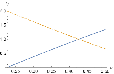
Figure 1: (Color online) Eigenvalue $\lambda_{I}$ (dashed, red line) and $\lambda_{Z}$ (bold, blue line) for the intermediate map Choi matrix of the non-Markovian dephasing channel characterized by Eq. (5). The intermediate $p$-range lies between $p{:=}p_{\ast}$ and $p{:=}p^{\ast}$, where $p_{\ast}<\alpha_{-}$, and $p^{\ast}$ is varied over the interval $[p_{\ast},\frac{1}{2}]$. At $p^{\ast}{:=}p_{\ast}$, $\lambda_{I}=2$ and $\lambda_{Z}=0$. At $p^{\ast}=\alpha_{-}$, the eigenvalues crossover, i.e., $\lambda_{I}=\lambda_{Z}=1$, and furthermore the channel becomes maximally dephasing, i.e., $\kappa=\frac{1}{2}$ in Eq. (5). Here, $\alpha:=0.3$ and $p_{\ast}:=\alpha_{-}-0.2\approx 0.23$.

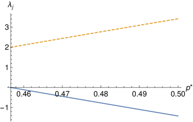
Figure 2: (Color online) Eigenvalue $\lambda_{I}$ (dashed, red line) and $\lambda_{Z}$ (bold, blue line) for the intermediate map Choi matrix of the non-Markovian dephasing channel characterized by Eq. (5). The intermediate $p$-range lies between $p{:=}p_{\ast}$ and $p{:=}p^{\ast}$, where $\frac{1}{2}>p_{\ast}>\alpha_{-}$, and $p^{\ast}$ is varied over the interval $[p_{\ast},\frac{1}{2}]$. For $p^{\ast}>p_{\ast}$, one finds $\lambda_{Z}<0$. Thus, the whole range $p^{\ast}\in(p_{\ast},\frac{1}{2}]$ corresponds to an NCP map, demonstrating the non-Markovianity of the channel characterized by Eq. (5). Here $\alpha:=0.3$ and $p_{\ast}:=\alpha_{-}+0.03\approx 0.46$.

III Negative decoherence rate in the master equation

The Kraus representation Eq. (5) is a solution to the master equation describing dephasing in the canonical form:

$$\frac{d\rho}{dp}=\gamma(p)(-\rho(p)+Z\rho(p)Z).$$ (16)

We now show that the decoherence rate corresponding to $\frac{1}{2}\geq p>\alpha_{-}$ is negative, indicative of non-Markovianity Hall et al. (2014). By direct substitution, and letting $G\equiv 1-2\kappa(p)$, one finds:

$$\gamma(p)=-\frac{1}{2G}\frac{dG}{dp}=\frac{\frac{1}{2}(\alpha_{+}+\alpha_{-})-p}{(p-\alpha_{-})(p-\alpha_{+})},$$ (17)

from which one sees that the evolution for $p<\alpha_{-}$ is Markovian ($\gamma\geq 0$), but becomes non-Markovian ($\gamma<0$) for $p>\alpha_{-}$. The point $\alpha_{-}$ itself represents a singularity (see Figure 3).

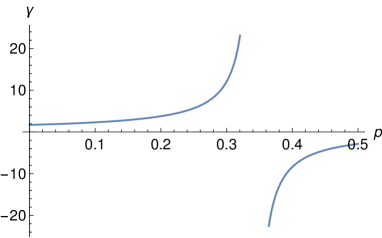
Figure 3: Plot of the decoherence rate $\gamma$ as a function of $p$ for $\alpha=0.7$. Note the singularity at $\alpha_{-}$ $(\approx 0.34)$, just after which $\gamma$ becomes negative, indicating that the evolution is non-Markovian.

Following Hall et al. (2014), we want to quantify the amount of non-Markovianity by $N_{\rm HCLA}\equiv-\int_{\alpha_{-}}^{1/2}\gamma(p)dp$, which however, would diverge because of the singularity at $\alpha_{-}$. One remedy, following an idea proposed in Rivas et al. (2014), is to replace $-\gamma(p)$ by its normalized version

$$\gamma^{\prime}\equiv\frac{-\gamma}{1-\gamma}=\frac{\alpha-2\alpha p+1}{\alpha-2\alpha p^{2}+2p},$$ (18)

from which we can define a normalized HCLA measure:

$$N_{\rm HCLA}^{\prime} \equiv\int_{\alpha_{-}}^{1/2}\gamma^{\prime}(p)dp$$

$$=\bigg{[}\frac{1}{2}\log\left(\alpha+2p-2\alpha p^{2}\right)$$

$$~{}~{}-\frac{\alpha\tan^{-1}\left(\frac{2\alpha p-1}{\sqrt{-2\alpha^{2}-1}}\right)}{\sqrt{-2\alpha^{2}-1}}\bigg{]}_{\alpha_{-}}^{1/2}$$ (19)

A plot of $N_{\rm HCLA}^{\prime}$ (bold line) is given in Figure 4. The monotonic increase of this measure with $\alpha$ justifies its being regarded as a non-Markovianity parameter. These results are directly related to the RHP measure, $N_{\rm RHP}$, of non-Markovianity Rivas et al. (2010), since $N_{\rm HCLA}=\frac{d}{2}N_{\rm RHP}$, where $d$ is system dimension Hall et al. (2014), which here is 2.

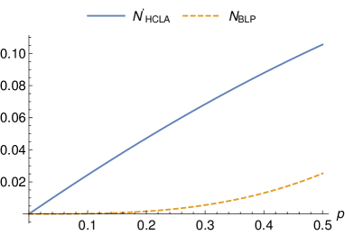
Figure 4: (Color online) Plot of the normalized HCLA coefficient $N_{\rm HCLA}^{\prime}$ (bold, blue line, Eq. (19)) and the BLP coefficient $N_{\rm BLP}$ (dashed, red line, Eq. (23)), as a function of the non-Markovian parameter $\alpha$.

IV The singularity isn’t pathological

The possible non-invertibility of the time evolution is discussed in Andersson et al. (2007); Rivas et al. (2014), in particular, the issue of general consistency conditions on such a map to derive a master equation, and the problem of quantification of non-Markovianity. In the present case, the singularity at $p=\alpha_{-}$ corresponds to a time where the trajectories of all initial states $\cos(\frac{\theta}{2})\ket{0}+e^{i\phi}\sin(\frac{\theta}{2})\ket{1}$ differing only by the azimuthal angle $\phi$, momentarily intersect. This is because the point $p=\alpha_{-}$ corresponds to maximal dephasing, under which any initial qubit state $\rho_{1}\equiv\begin{pmatrix}a&b\\ b^{\ast}&1-a\end{pmatrix}$ is transformed to $\rho_{2}\equiv\begin{pmatrix}a&0\\ 0&1-a\end{pmatrix}$. In other words, all off-diagonal terms in the computational basis are killed off, making the map momentarily non-invertible. Nevertheless, the singularity isn’t pathological, in the sense that the density operator, and consequently the full map, are well defined, and invertibility is subsequently recovered.

At time $\alpha_{-}$, the intermediate dynamical map Eq. (15) advancing the state by a small time interval $\epsilon$, is acting on a density operator of the type $\rho_{2}$ and induces the intermediate evolution:

$$\rho_{2} \longrightarrow\frac{(1+Y)}{2}\rho_{2}+\frac{(1-Y)}{2}Z\rho_{2}Z$$

$$=\frac{(1+Y)}{2}\rho_{2}+\frac{(1-Y)}{2}\rho_{2}=\rho_{2},$$ (20)

where $Y\equiv\frac{\left(\alpha_{-}-p^{\ast}\right)\left(\alpha_{+}-p^{\ast}\right)}{\left(\alpha_{-}-p_{\ast}\right)\left(\alpha_{+}-p_{\ast}\right)}$ is the divergent summand in the expression for $K_{I}^{\rm int}$ in Eq. (15) and we set $p_{\ast}{:=}\alpha_{-}$. Since the singularity in the intermediate map occurs at the point of maximal dephasing, the infinite term $Y$ has no effect, as it would only multiply with off-diagonal terms in the density operator, which vanish.

Similarly, in the master equation (16) for the rate $\frac{d\rho}{dp}$, we note that the divergence of $\gamma(p)$ at the singularity is rendered harmless by virtue of the fact that the term $\rho(\alpha_{-})-Z\rho(\alpha_{-})Z$, which it multiplies, vanishes for the above reason.

V Quantifying non-Markovianity via trace distance

There are a host of measures to witness or quantify non-Markovianity, such as trace distance, fidelity, quantum relative entropy, quantum Fisher information, capacitance measures; as well as correlation measures such as mutual information, entanglement, and discord, all of which are non-increasing under CP-divisible maps, and can thus be used to witness non-Markovianity Rivas et al. (2010).

Here, we consider evolution of the trace distance (TD) Breuer et al. (2009), applied to the pair of initial states: $\ket{\psi_{0}}=\cos(\theta/2)\ket{0}+e^{i\phi}\sin(\theta/2)\ket{1}$ and $\ket{\psi_{1}}=-\sin(\theta/2)\ket{0}+e^{i\phi}\cos(\theta/2)\ket{1}$. For this pair:

$${\rm TD}(\theta,\phi,\alpha,p) \equiv\frac{1}{2}{\rm tr}\sqrt{(\rho_{0}-\rho_{1})^{2}}$$

$$=\bigg{[}1-4\alpha^{2}(1-p)p(\alpha_{+}+\alpha_{-}-p)\times$$

$$\quad\quad(2\alpha_{+}\alpha_{-}-p)\sin^{2}(\theta)\bigg{]}^{1/2},$$ (21)

where $\rho_{j}=\mathcal{E}(\ket{\psi_{j}}\bra{\psi_{j}})$, and $\mathcal{E}$ represents the time evolution under our non-Markovian dephasing. The expression is independent of $\phi$, reflecting the azimuthal symmetry of the dephasing action Banerjee and Ghosh (2007); Banerjee and Srikanth (2008). For $\theta$ where $0<\theta<2\pi$, it may be seen that TD attains a minimum of $\cos(\theta)$ at $\alpha_{-}$. The subsequent ($p>\alpha_{-}$) rise in TD signals non-Markovianity.

This pattern is manifest in the case of $\theta=\frac{\pi}{2}$, for which Eq. (21) reduces to the particularly simple form

$${\rm TD}_{\pi/2}(p)=2\alpha\left(p-\alpha_{-}\right)\left(p-\alpha_{+}\right).$$ (22)

This is depicted in Figure 5 for various non-Markovian parameters $\alpha$. We note in this Figure that the recurrence region $(\alpha_{-},\frac{1}{2}]$ is larger for larger $\alpha$, suggestive of greater non-Markovianity for larger $\alpha$.

The BLP measure of non-Markovianity, denoted $N_{\rm BLP}$, is given by:

$$N_{\rm BLP} =\max_{(\psi_{0},\psi_{1})}\int_{\alpha_{-}}^{1/2}\frac{d{\rm TD}}{dp}dp$$

$$=\max_{\theta}\bigg{[}\sqrt{1+(-1+\frac{\alpha^{2}}{4})\sin^{2}(\theta)}-\cos(\theta)\bigg{]}$$

$$=\frac{\alpha}{2}.$$ (23)

The result is depicted as the dashed (red) line in Figure 4, and shows that there is a general agreement with the quantification of non-Markovianity according to the normalized HCLA measure $N_{\rm HCLA}^{\prime}$.

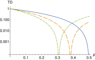
Figure 5: Log plot of trace distance TD between $\rho_{0}\equiv\mathcal{E}(\ket{\psi_{0}}\bra{\psi_{0}})$ and $\rho_{1}\equiv\mathcal{E}(\ket{\psi_{1}}\bra{\psi_{1}})$ as a function of $p$ with $\theta{:=}\frac{\pi}{2}$, under the considered non-Markovian dephasing noise. The bold (blue) curve represents Markovian dephasing, and shows no recurrence. The dashed (red, $\alpha=0.5)$ and dot-dashed (green, $\alpha=0.9$) show enhanced distinguishability beyond their respective crossover point $\alpha_{-}$, indicative of non-Markovianity. Note that larger $\alpha$ shows a larger enhancement region, suggesting larger non-Markovianity in the sense of BLP Breuer et al. (2009).

Here, following Breuer et al. (2009), we have assumed that the pair of states parametrized by $(\theta,\phi)$, is orthogonal. This is appropriate, to enhance the contrast that demonstrates non-Markovianity. Specifically, note that the TD in Figure 5 varies in the range between 1 (initial) and 0 (maximal dephasing). If, on the other hand, the two initial stats were (say) $\ket{0}$ and $\frac{1}{\sqrt{2}}(\ket{0}+\ket{1})$, then TD varies in the smaller range between $\frac{1}{\sqrt{2}}$ (initial) and $\frac{1}{2}$ (maximal dephasing).

VI Non-Markovian Depolarizing

The depolarizing channel of a qubit transforms state $\rho$ to a mixture of itself and the maximally mixed state. The non-Markovian version of the depolarizing channel can also be found in a manner analogous to the dephasing channel, which is now discussed briefly.

A Kraus representation for the depolarizing channel would be $\rho\longrightarrow\sum_{j}K_{j}\rho K_{j}^{\dagger}$, where $K_{I}=\sqrt{1-p}I$, $K_{X}=\sqrt{\frac{p}{3}}X$, $K_{Y}=\sqrt{\frac{p}{3}}Y$ and $K_{Z}=\sqrt{\frac{p}{3}}Z$. A potential non-Markovian extension for them would be

$$K_{I} =\sqrt{(1+\Lambda_{1})(1-p)}\;\quad K_{X}=\sqrt{(1+\Lambda_{2})\frac{p}{3}}X$$

$$K_{Y} =\sqrt{(1+\Lambda_{2})\frac{p}{3}}Y;\quad K_{Z}=\sqrt{(1+\Lambda_{2})\frac{p}{3}}Z$$ (24)

where $\Lambda_{k}$ ($k\in\{1,2\}$) is a real function, and $p$ is a timelike parameter that rises monotonically from 0 to $\frac{1}{2}$. The variables $\Lambda_{j}$ satisfy the following condition,

$$(1-p)\,\Lambda_{1}+p\,\Lambda_{2}=0$$ (25)

as a consequence of the completeness requirement.

In agreement with Eq. (25), we make the following choices: $\Lambda_{1}=-3\alpha p$ and $\Lambda_{2}=3\alpha(1-p)$, where $\alpha$ is real. Then, the non-Markovian Kraus operators take the form

$$K_{I}(p) =\sqrt{[1-3\alpha p](1-p)}\;I$$

$$K_{X}(p) =\sqrt{[1+3\alpha(1-p)]\frac{p}{3}}X,$$

$$K_{Y}(p) =\sqrt{[1+3\alpha(1-p)]\frac{p}{3}}Y,$$

$$K_{Z}(p) =\sqrt{[1+3\alpha(1-p)]\frac{p}{3}}Z,$$

As before, parameter $\alpha$ may be seen to represent the non-Markovian behavior of the channel, such that setting $\alpha:=0$ reduces the Kraus operators in Eq. (LABEL:eq:nmdepol2) to those in the conventional Markovian depolarization channel.

VII Conclusions and discussion

We introduced a method to construct non-Markovian variants of completely positive (CP) dynamical maps, particularly, qubit Pauli channels, with non-Markovianity defined by departure from CP-divisibility. Specifically, a one-parameter non-Markovian dephasing channel was studied in detail, which is characterized by a singularity in the canonical decoherence rate $\gamma$, which occurs at the crossover point $\alpha_{-}$ associated with the eigenvalues of the intermediate map, and where phase noise is maximal. The decoherence rate $\gamma$ is negative for $p\in(\alpha_{-},\frac{1}{2}]$, indicating non-Markovianity. Intuitively, this can be understood as due to $\kappa$ in Eq. (1) exceeding $\frac{1}{2}$, thereby enhancing distinguishability.

More precisely, substituting the form Eq. (1) into Eq. (16), one finds that:

$$\gamma=\frac{d\kappa/dp}{1-2\kappa},$$ (27)

which relates the “channel mixing rate” $\frac{d\kappa}{dp}$ to the decoherence rate $\gamma$. From Eq. (27), it follows that

$$\gamma<0{\rm~{}iff~{}}\bigg{\{}\begin{array}[]{ll}\frac{d\kappa}{dp}<0,&{\rm~{}in~{}case~{}of~{}}\kappa<\frac{1}{2}\\ \frac{d\kappa}{dp}>0,&{\rm~{}in~{}case~{}of~{}}\kappa>\frac{1}{2},\end{array}$$ (28)

with $\kappa=\frac{1}{2}$ representing a singularity. In the form of noise we consider, the second case in Eq. (28) explains the origin of non-Markovianity. The reason is that the derivative of the “channel mixing parameter” $\kappa$ is always positive, i.e., $\frac{d\kappa}{dp}>0$. Thus, $\kappa(p)$ must exceed $\frac{1}{2}$ for non-Markovianity to occur. In view of Eq. (27), this entails that a singularity must be encountered when $\kappa=\frac{1}{2}$, which happens in our case at $p=\alpha_{-}$.

This is illustrated by the dashed (red) plot in Figure 6, which represents our non-Markovian dephasing with $\alpha=0.7$, for which $\frac{d\kappa}{dp}>0$ throughout the range $[0,\frac{1}{2}]$. The point $\alpha_{-}$, where this intercepts the horizontal line of $\kappa=\frac{1}{2}$, is the singularity. Non-Markovianity comes from the positive mixing rate ($\frac{d\kappa}{dp}>0$) region $p>\alpha_{-}$.

On the other hand, non-Markovian dephasing noise where $\kappa$ remains within $[0,\frac{1}{2}]$ as $p$ increases monotonically from 0 to $\frac{1}{2}$, corresponds to the first case in Eq. (28). Here, the channel mixing parameter can’t monotonically rise, i.e., there must be regions where $\frac{d\kappa}{dp}<0$. As a simple instance, consider:

$$\kappa(p)=p\frac{\left(1+\eta\sin(\omega p)(1-2p)\right)}{\left(1+\eta(1-2p)\right)},$$ (29)

with $0\leq p\leq\frac{1}{2}$, where $\eta$ and $\omega$ are positive constants characterizing the strength and frequency of the channel.

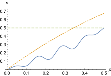
Figure 6: Plot of $\kappa(p)$ in Eq. (29) as a function of $p$, with $\eta=\frac{1}{2}$ and $\omega=50$ (bold, blue line). This dephasing channel corresponds to the first case of Eq. (28) and non-Markovianity arises from regions of negative slope in the plot. The dashed (red) line corresponds to the non-Markovian dephasing Eq. (5) with $\alpha=0.7$. The mixing rate $d\kappa/dp$ is never negative, and non-Markovianity pertains to the first case in Eq. (28).

Such a noisy channel encounters no singularity, and the non-Markovian contributions come from the regions of negative mixing rate $\frac{d\kappa}{dp}$, which arises because of the sine function. A plot of $\kappa(p)$ for $\eta=\frac{1}{2}$ and $\omega=50$ is the bold (blue) plot in Figure 6.

We discussed two methods of quantifying the non-Markovianity, one based on CP-divisibility and another on distinguishability. The former is derived from the HCLA measure Hall et al. (2014), based on negative decoherence rates in the canonical master equation. This doesn’t require optimization but is marked by a singularity, which we have handled by using a suitable normalization. The other measure is the BLP measure Breuer et al. (2009), which requires optimization but is unaffected by the singularity.

Our method to construct a non-Markovian variant of the dephasing channel can be straightforwardly extended to other Pauli channels, e.g., bit flip or depolarizing channels. Details such as the level-crossing feature of the eigenvalues of the Choi matrix of intermediate map and the occurence of singularities, may vary from case to case, presenting new insights.