A transformed stochastic Euler scheme for multidimensional transmission PDE

Abstract

In this paper we consider multi-dimensional Partial Differential Equations (PDE) of parabolic type in divergence form. The coefficient matrix of the divergence operator is assumed to be discontinuous along some smooth interface. At this interface, the solution of the PDE presents a compatibility transmission condition of its co-normal derivatives (multi-dimensional diffraction problem). We prove an existence and uniqueness result for the solution and study its properties. In particular, we provide new estimates for the partial derivatives of the solution in the classical sense. We then construct a low complexity numerical Monte Carlo stochastic Euler scheme to approximate the solution of the PDE of interest. Using the afore mentioned estimates, we prove a convergence rate for our stochastic numerical method when the initial condition belongs to some iterated domain of the divergence form operator. Finally, we compare our results to classical deterministic numerical approximations and illustrate the accuracy of our method.

1 Introduction

Given a finite time horizon $T$, a real valued function $x\mapsto u_{0}(x)$, and an elliptic symmetric matrix $x\mapsto a(x)\in\mathbb{R}^{d\times d}$, which is smooth except at the interface surface $\Gamma$ between subdomains $D_{\pm}$ of $\mathbb{R}^{d}$ ($\Gamma=\bar{D}_{+}\cap\bar{D}_{-}$), we consider the parabolic transmission (or diffraction) problem : find $u$ from $[0,T]\times\mathbb{R}^{d}$ to $\mathbb{R}$ satisfying

$$\left\{\begin{array}[]{l}\partial_{t}u(t,x)-\nabla.\left(a(x)\nabla_{x}u(t,x)\right)=0,\leavevmode\nobreak\ \;\forall(t,x)\in(0,T]\times(\mathbb{R}^{d}\setminus\Gamma)\\ \\ u(0,x)=u_{0}(x),\;\forall x\in\mathbb{R}^{d}\\ \\ \langle a_{+}\nabla_{x}u_{+}(t,.)-a_{-}\nabla_{x}u_{-}(t,.),\nu\rangle=0\text{ and }u_{+}(t,.)=u_{-}(t,.)\;\text{ along }\Gamma.\\ \end{array}\right.$$ (1.1)

The objective of this paper is to provide an efficient stochastic numerical resolution method for the solution of (1.1).

Parabolic equations involving $\nabla\cdot\left(a\nabla\right)$ have been a major preoccupation for mathematicians in the fifties and the sixties. We may cite the pioneering works of [39, 38], [5], and [35, 36, 37] that prove the continuity of the solution of the Cauchy problem attached to $\nabla\cdot\left(a\nabla\right)$ and also the celebrated paper by [1], which gives upper and lower Gaussian estimate bounds for the fundamental solution of the operator $\nabla\cdot\left(a\nabla\right)$ (for a more modern perspective on evolution PDEs involving divergence form operators of type $\nabla\cdot\left(a\nabla\right)$ see also [30]). In these references assumptions on $a$ are very weak (it is assumed to be measurable, bounded and elliptic).

In the case where the matrix $a$ is assumed to be discontinuous along the regular boundaries of some nice disjoint connected open sets in $\mathbb{R}^{d}$, but smooth elsewhere, a refined analysis of the parabolic equation may be found in the monograph [20]. The authors interpret the parabolic equation as a diffraction problem with transmission conditions along the discontinuity boundaries, of the type of (1.1), and investigate the classical smoothness of its solution.

When the underlying space is one-dimensional and the discontinuity is at zero ($\Gamma$ then reduces to the single point $0$), the link between (1.1) and some asymmetric diffusion process $X$ is well known. More precisely one has that $u(t,x)=\mathbb{E}^{x}[u_{0}(X_{t})]$ where $X$ is solution to the Stochastic Differential Equation (SDE) with local time

$$dX_{t}=\sigma(X_{t})dW_{t}+a^{\prime}(X_{t})dt+\frac{a(0+)-a(0-)}{a(0+)+a(0-)}dL_{t}^{0}(X)$$ (1.2)

where $\sigma^{2}=2a$ and $a^{\prime}$ denotes a function that coincides with the first order derivative of $a$ outside zero, and can be set at any arbitrary value at zero. In (1.2) we have denoted $W$ a standard one-dimensional Brownian motion (B.m.), and $L_{t}^{0}(X)$ the symmetric local time of $X$ at time $t$. Under mild conditions (1.2) has a unique strong solution $X$, see [22]. Put in other words the operator $\nabla\cdot\left(a\nabla\right)$ appears as the infinitesimal generator of the diffusion $X$ solution of (1.2). Note that the local time term in (1.2) is a singular term that reflects the discontinuity of $a$ along $\Gamma=\{0\}$.

For a study of the one-dimensional case one may refer to the overview [23], [12], and the series of works [31, 32, 33, 26, 7, 8, 10, 11] [25, 6, 14, 24] where stochastic numerical schemes are presented.

Then if one constructs a scheme $\overline{X}$ approaching $X$ (in law for example), we will have that $\mathbb{E}^{x}[u_{0}(\overline{X}_{t})]$ approaches $u(t,x)$. This provides some stochastic numerical resolution method for the solution of (1.1). But none of the above cited works on the one-dimensional case can be directly adapted to the multidimensional case.

As a matter of fact, till now and up to our knowledge much fewer stochastic schemes have been proposed and studied to tackle the multidimensional case.

A natural idea would be to regularize the coefficient $a$ around the interface $\Gamma$, and then to perform a discretized stochastic scheme on the classical problem obtained by regularization (for smooth $a^{\varepsilon}$ the process $X$ in link with $\nabla\cdot\left(a^{\varepsilon}\nabla\right)$ is some Itô process with classical drift that can be approached by a standard Euler scheme). But then there is a balance to find between the regularization step and the discretization step. Such methods are less precise and less investigated (see [41] for some elements in this direction; see also some of our numerical results in Section 6).

For some results with no regularization procedure see [27], and [2] in the case of a diagonal coefficient matrix $a$ constant outside the discontinuity boundary $\Gamma$; see also [29], which attempts to interpret stochastically the deterministic Galerkin method using jump Markov Chains.

In this paper we will propose a stochastic numerical scheme that allows to treat the multidimensional case, when the matrix-valued diffusion coefficient $a$ is not necessarily diagonal, nor piecewise constant. We aim at treating the discontinuity of $a$ directly and use no regularization. The scheme we propose is of Euler type; it can be seen as en extension to the multidimensional case of the scheme studied in [33] (see some comments in Remark 4.4).

One of the difficulties of the multidimensional case is that the stochastic process $X$ naturally in link with the operator $\nabla\cdot\left(a\nabla\right)$ is more difficult to describe than in dimension one. One knows that the operator generates such a process $X$, which is Markov (see for instance [40]; on the Dirichlet form approach see [15], in particular Exercise 3.1.1 p111). We still have the link $u(t,x)=\mathbb{E}^{x}[u_{0}(X_{t})]$. But the Itô dynamic of $X$ is difficult to establish and to exploit. In the companion paper [9] we have been able to prove (in the case $\mathbb{R}^{d}=\bar{D}_{+}\cup D_{-}$ and $a$ has some smoothness in $D_{\pm}$) that

$$X_{t}^{k} =x_{k}+\int_{0}^{t}\sum_{j=1}^{d}\sigma_{kj}(X_{s})dW_{s}^{j}+\int_{0}^{t}\sum_{j=1}^{d}\partial_{j}a_{kj}(X_{s}){\mathbb{I}}_{\mathnormal{X_{s}\in D}}ds$$

$$\hskip 14.22636pt-\frac{1}{2}\int_{0}^{t}\gamma_{+,k}(X_{s})dK_{s}+\frac{1}{2}\int_{0}^{t}\gamma_{-,k}(X_{s})dK_{s},\hskip 8.5359ptt\geq 0.$$ (1.3)

In this expression $W$ is a standard B.m., we have $\sigma\sigma^{*}=2a$, the terms $\gamma_{\pm,k}$ are some co-normal vectors to the surface $\Gamma=\bar{D}_{+}\cap\bar{D}_{-}$, and $K$ is the PCAF associated through the Revuz correspondence to the surface measure on $\Gamma$. Equation (1) is in some sense the multi-dimensional analog to (1.2), the singular term being now $-\frac{1}{2}\int_{0}^{t}\gamma_{+,k}(X_{s})dK_{s}+\frac{1}{2}\int_{0}^{t}\gamma_{-,k}(X_{s})dK_{s}$.

However to infer from (1) an approximation scheme $\overline{X}$ for $X$ is not easy. In the afore mentioned works about the one-dimensional case, things are most often achieved with the help of Itô-Tanaka type formulas, that allow to manipulate SDEs with local time. In the multi-dimensional case we have not access to such a formula, and in addition we know less about the singular term $-\frac{1}{2}\int_{0}^{t}\gamma_{+,k}(X_{s})dK_{s}+\frac{1}{2}\int_{0}^{t}\gamma_{-,k}(X_{s})dK_{s}$ than we know about $L^{0}_{t}(X)$ in the one-dimensional case.

Thus we are led, in the present paper, to contruct a stochastic scheme $\overline{X}$ such that $\mathbb{E}^{x}[u_{0}(\overline{X}_{t})]$ approaches $u(t,x)$, but without seeking to approach $X$ by $\overline{X}$. The idea will be to perform a standard Euler scheme as long as $\overline{X}$ does not cross the boundary $\Gamma$. But when the scheme $\overline{X}$ crosses the boundary we will correct its position in a way that reflects the transmission condition in (1.1). The contribution of the paper are the following.

I) We will first study the PDE (1.1). We will show that, when the initial condition $u_{0}$ belongs to some iteration of the domain of $\nabla\cdot\left(a\nabla\right)$, this PDE has a classical solution. Then we prove the existence of global bounds for the partial derivatives of this solution (up to order four in the space variable) outside the discontinuity boundary $\Gamma$, for all strictly positive times (and not just for times $t$ satisfying $t\geq\varepsilon$ for some $\varepsilon>0$), and all the way up to the boundary (not only interior estimates). In our opinion these estimates are new (compared to [20]) and have an interest per se. These estimates will be needed to perform the convergence analysis of our scheme. The method we follow, in this PDE oriented part of the paper, is combining the Hille-Yosida theorem with results on elliptic transmission PDEs to be found in [34].

II) We propose our scheme (we insist again that our matrix valued coefficient $a$ does not need to be diagonal) and study its convergence rate. More precisely we prove that

$$\Big{|}u(T,x_{0})-\mathbb{E}^{x_{0}}u_{0}(\overline{X}^{n}_{T})\Big{|}\leq K\sqrt{h_{n}},$$

where $h_{n}$ is the time step of our Euler scheme (see the precise assumptions and statement in Theorem 5.1). This has to be compared with the results in the classical smooth case and the ones in [33].

The paper is organised as follows. In Section 2 we present the notations of the paper and our main assumptions. In Section 3 we define precisely and study the parabolic transmission problem (1.1), proving in particular an existence and uniqueness result for a classical solution, for which we get estimates for the space and time derivatives. In Section 4 we present our scheme, and in Section 5 we analyse its convergence. Section 6 is devoted to numerical experiments.

2 General notations and assumptions

For two points $x,y\in\mathbb{R}^{d}$ we denote by $\langle x,y\rangle$ their scalar product $\langle x,y\rangle=x^{*}y=\sum_{i=1}^{d}x_{i}y_{i}$.

For a point $x\in\mathbb{R}^{d}$ we denote by $|x|$ its Euclidean norm i.e. $|x|^{2}=\sum_{i=1}^{d}x_{i}^{2}=\langle x,x\rangle$.

We denote by $(e_{1},\ldots,e_{d})$ the usual orthonormal basis of $\mathbb{R}^{d}$.

For two metric spaces $E,F$ we will denote by $C(E;F)$ the set of continuous functions from $E$ to $F$ and, for $1\leq p\leq\infty$, by $C^{p}(E;F)$ the set of functions in $C(E;F)$ that are $p$ times differentiable with continuous derivatives.

We will denote by $C^{p}_{c}(E;F)$ the set of functions in $C^{p}(E;F)$ that have a compact support.

We will denote by $C^{p}_{b}(E;F)$ the set of functions in $C^{p}(E;F)$ that are continuous with bounded $p$ first derivatives ($C_{b}(E;F)$ denotes the set of functions in $C(E;F)$ that are bounded).

If $F=\mathbb{R}$, we will sometimes simply write for instance $C(E)$ for $C(E;\mathbb{R})$, for the sake of conciseness.

For any multi-index $\alpha=(i_{1},\dots,i_{d})\in\mathbb{N}^{d}$ and $x=(x_{1},\dots,x_{d})\in\mathbb{R}^{d}$, we note $x^{\alpha}$ the product $x_{1}^{i_{1}}\dots x_{d}^{i_{d}}$ and $|\alpha|=i_{1}+\dots+i_{d}$. So that for $u\in C^{|\alpha|}(\mathbb{R}^{d})$ we will denote $\frac{\partial^{|\alpha|}u}{\partial x^{\alpha}}$, or in short $\partial^{\alpha}u$, the partial derivative $\partial^{i_{1}}_{x_{1}^{i_{1}}}\ldots\partial^{i_{d}}_{x_{d}^{i_{d}}}u$.

Let $U\subset\mathbb{R}^{d}$ an open subset. We will denote by $L^{2}(U)$ the set of square integrable functions from $U$ to $\mathbb{R}$ equipped with the usual norm and scalar product $||\cdot||_{L^{2}(U)}$ and $\langle\cdot,\cdot\rangle_{L^{2}(U)}$.

We denote $H^{1}(U)$ the usual Sobolev space $W^{1,2}(U)$, equipped with the usual norm $||\cdot||_{H^{1}(U)}$. We will denote by $D_{i}v$ the derivative in the distribution sense with respect to $x_{i}$ of $v\in L^{2}(U)$.

We recall that the space $H^{1}_{0}(U)\subset H^{1}(U)$ can be defined as $H^{1}_{0}(U)=\overline{C^{\infty}_{c}(U;\mathbb{R})}=\overline{C^{1}_{c}(U;\mathbb{R})}$.

We denote $H^{-1}(U)$ the usual dual topological space of $H^{1}_{0}(U)$.

For $m\geq 2$, we denote $H^{m}(U)$ the usual Sobolev space $W^{m,2}(U)\subset L^{2}(U)$ of functions having $m$ successive weak derivatives in $L^{2}(U)$.

The notion of a $C^{k}$ domain $U\subset\mathbb{R}^{d}$ with bounded boundary $\Gamma=\partial U$ is defined with the help of a system of local change of coordinates of class $C^{k}$ (see [34] Chap.3 pp89-90).

From now on we consider in the whole paper that $\mathbb{R}^{d}=\bar{D}_{+}\cup D_{-}$ with $D_{+}$ and $D_{-}$ two open connected subdomains separated by a transmission boundary $\Gamma$ that is to say

$$\Gamma=\bar{D}_{+}\cap\bar{D}_{-}$$

(in addition we will denote $D=D_{+}\cup D_{-}=\mathbb{R}^{d}\setminus\Gamma\subset\mathbb{R}^{d}$).

By an assumption of type ”$\Gamma$ is bounded and $C^{k}$” we will mean that both $D_{+}$ and $D_{-}$ are $C^{k}$ domains, and that $\Gamma$ is bounded. Note that in that case we shall consider $D_{+}$ (resp. $D_{-}$) as the interior (resp. exterior) domain. Note that $D_{-}$ is then unbounded (although its boundary is bounded).

Assume $\Gamma$ is bounded and $C^{2}$. We will denote $\gamma:H^{1}(D_{\pm})\to H^{1/2}(\Gamma)$ the usual trace operator on $\Gamma$ and $H^{-1/2}(\Gamma)$ the dual space of $H^{1/2}(\Gamma)$ (see p98-102 in [34]).

In the sequel we will frequently note $f_{\pm}$ the restrictions of a function $f$ to $D_{\pm}$. Besides, by an assumption of type ”the function $f$ satisfies $f_{\pm}\in C^{p}(\bar{D}_{\pm})$” (or ”$f\in C^{p}(\bar{D}_{+})\cap C^{p}(\bar{D}_{-})$”) we will mean that the restriction of $f$ to $D_{+}$ (resp. $D_{-}$) coincides on $D_{+}$ (resp. $D_{-}$) with a function $\tilde{f}_{+}$ of class $C^{p}(\mathbb{R}^{d})$ (resp. $\tilde{f}_{-}$). So that for any $x\in\Gamma$ we can give a sense for example to $f_{+}(x)$: it is $\lim_{z\to x\,,\,z\in D_{+}}f(z)=\tilde{f}_{+}(x)$.

In the same time spirit we may note for $f\in C(\bar{D}_{+})\cap C(\bar{D}_{-})$ and a point $y\in\Gamma$

$$f(y\pm)=\lim_{z\to y\,,\,z\in D_{\pm}}f(z)=f_{\pm}(y).$$

For $u\in C^{1}(\bar{D}_{+};\mathbb{R})\cap C^{1}(\bar{D}_{-};\mathbb{R})$ we denote $\nabla_{x}u=(\frac{\partial u}{\partial x_{1}},\ldots,\frac{\partial u}{\partial x_{d}})^{\ast}$ and, for a point $y\in\Gamma$

$$\nabla_{x}u_{\pm}(y)=\lim_{z\to y\,,\,z\in D_{\pm}}\nabla_{x}u(z).$$ (2.1)

For a vector field $G\in C^{1}(D;\mathbb{R}^{d})$ we denote by $\nabla\cdot G\,(x)$ its divergence at point $x\in D$, i.e. $\nabla\cdot G(x)=\sum_{i=1}^{d}\frac{\partial G_{i}}{\partial x_{i}}(x)$.

For $u\in C^{2}(D;\mathbb{R})$ and $x\in D$ we denote $\mathbf{H}[u](x)$ the Hessian matrix of $u$ at point $x$.

Let $a(x)=(a_{ij}(x))_{i,j\in\{1,\dots,d\}}$ be a symmetric matrix valued and time homogeneous diffusion coefficient.

If $a_{ij}\in C^{1}(D;\mathbb{R})$ for all $1\leq i,j\leq d$ and $u\in C^{2}(D;\mathbb{R})$ we denote

$${\cal L}u(x)=\nabla\cdot\left(a(x)\nabla_{x}u(x)\right),\quad\forall x\in D.$$ (2.2)

In the whole paper the coefficients of the function matrix $a$ are always assumed to be measurable and bounded by a constant $\Lambda$.

We will also often make the following ellipticity assumption

Assumption 2.1.

(E) : There exists $\lambda\in(0,\infty)$ such that

$$\forall x\in\mathbb{R}^{d},\;\;\forall\xi\in\mathbb{R}^{d},\quad\lambda|\xi|^{2}\leq\xi^{\ast}a(x)\xi.$$ (2.3)

Note that under $(\mathbf{E})$ we can assert that for any $x\in D$ we have

$$a_{\pm}(x)=P_{\pm}^{*}(x)E_{\pm}(x)P_{\pm}(x)$$ (2.4)

with $P_{\pm}(x)$ some orthogonal matrices and $E_{\pm}(x)$ some diagonal matrices with strictly positive eigenvalues.

Assume $\Gamma$ is $C^{2}$. For a point $x\in\Gamma$ we denote by $\nu(x)\in\mathbb{R}^{d}$ the unit normal to $\Gamma$ at point $x$, pointing to $D_{+}$. Assume the $a_{ij}$’s satisfy $(a_{\pm})_{ij}\in C(\bar{D}_{\pm})$. We define then the co-normal vector fields ${\gamma_{+}}(x):=a_{+}(x)\nu(x)$ and $\gamma_{-}(x):=-a_{-}(x)\nu(x)$, for $x\in\Gamma$.

Note that under $(\mathbf{E})$ it is clear that we have

$$\forall x\in\Gamma,\hskip 8.5359pt\langle{\gamma_{+}}(x),\nu(x)\rangle\geq\lambda>0\hskip 8.5359pt\text{and}\hskip 8.5359pt\langle\gamma_{-}(x),\nu(x)\rangle\leq-\lambda<0.$$ (2.5)

Note that the notation $\gamma$ for the trace operator follows the usual one ([34] for instance) and the notation $\gamma_{\pm}$ for the co-normal vectors follows the one of the paper [3]. But it will be dealt with the trace operator only in Section 3, and with co-normal vectors only in Sections 4 and 5. So that these notations will cause no confusion.

To finish with we define the unbounded operator $A:\mathcal{D}(A)\subset L^{2}(\mathbb{R}^{d})\to L^{2}(\mathbb{R}^{d})$ by

$$\mathcal{D}(A)=\big{\{}u\in H^{1}(\mathbb{R}^{d})\text{ with }\sum_{i,j=1}^{d}D_{i}(a_{ij}D_{j}u)\in L^{2}(\mathbb{R}^{d})\big{\}}$$

and

$$\forall u\in\mathcal{D}(A),\quad Au=\sum_{i,j=1}^{d}D_{i}(a_{ij}D_{j}u).$$

Then we introduce the iterated domains defined recursively by

$$\mathcal{D}(A^{k})=\{v\in\mathcal{D}(A^{k-1}):\;\;Av\in\mathcal{D}(A^{k-1})\},\quad k\geq 2.$$

3 The parabolic transmission problem

Let $0<T<\infty$ a finite time horizon. Let us consider the transmission parabolic problem

$$(\mathcal{P}_{\mathrm{T}})\left\{\begin{array}[]{rcll}\partial_{t}u(t,x)-\mathcal{L}u(t,x)&=&0&\forall(t,x)\in(0,T]\times D\\ \\ \langle a_{+}\nabla_{x}u_{+}(t,y)-a_{-}\nabla_{x}u_{-}(t,y),\nu(y)\rangle&=&0&\forall(t,y)\in(0,T]\times\Gamma\quad(\star)\\ \\ u(t,y+)&=&u(t,y-)&\forall(t,y)\in[0,T]\times\Gamma\\ \\ u(0,x)&=&u_{0}(x)&\forall x\in\mathbb{R}^{d}.\\ \end{array}\right.$$

We will say that $(t,x)\mapsto u(t,x)$ is classical solution to $(\mathcal{P}_{\mathrm{T}})$ if it satisfies

$$u\!\in\!C\big{(}[0,T];C^{2}(\bar{D}_{+})\cap C^{2}(\bar{D}_{-})\big{)}\cap C^{1}\big{(}[0,T];C(\bar{D}_{+})\cap C(\bar{D}_{-})\big{)}\cap C\big{(}[0,T];C(\mathbb{R}^{d})\big{)}$$ (3.1)

and satisfies the following requisites. First, $u$ satisfies the first line of $(\mathcal{P}_{\mathrm{T}})$, where the derivatives are understood in the classical sense. Second, for all $0<t\leq T$ the limits $\lim_{z\to y\,,\,z\in D_{\pm}}\nabla_{x}u(t,z)$ satisfy the transmission condition $(\star)$ for all $y\in\Gamma$. Note that these limits exist thanks to (3.1). Third, $u$ is continuous accross $\Gamma$ (third line). Fourth, it satisfies the initial condition at the fourth line of $(\mathcal{P}_{\mathrm{T}})$.

The aim of this section is to prove the following result.

Theorem 3.1.

Let $a=(a_{ij})_{1\leq i,j\leq d}$ satisfy $(\mathbf{E})$.

• Denote

  $$k_{0}=\left\{\begin{array}[]{l}\lfloor{\frac{d}{4}}\rfloor+2\;\;\text{ if }d\text{ is even;}\\ \lfloor{\frac{3}{2}+\frac{\lfloor{d/2}\rfloor}{2}}\rfloor+2\;\;\text{ if }d\text{ is odd.}\end{array}\right.$$ (3.2)

  Assume that the coefficients $a_{ij}$ satisfy $(a_{\pm})_{ij}\in C_{b}^{2k_{0}-3}(\bar{D}_{\pm})$ and $\Gamma$ is bounded and of class $C^{2k_{0}-2}$. Then for $u_{0}\in\mathcal{D}(A^{k_{0}})$ the parabolic transmission problem $(\mathcal{P}_{\mathrm{T}})$ admits a classical solution.

• Furthermore, if $u_{0}\in\mathcal{D}(A^{k})$ for $k\geq k_{0}$, the coefficients $a_{ij}$ satisfy $(a_{\pm})_{ij}\in C_{b}^{2k-1}(\bar{D}_{\pm})$ and $\Gamma$ is bounded of class $C^{2k}$, this classical solution $u$ is such that

  $$u\in C^{k-j}\left([0,T]\;;\;C^{n(j)}(\bar{D}_{+})\cap C^{n(j)}(\bar{D}_{-})\right),\quad\lceil d/4\rceil\leq j\leq k$$

  with $n(j)=\lfloor 2j-\frac{d}{2}\rfloor$.

To prove Theorem 3.1 requires to study in a first time the associated elliptic resolvent equation, in a weak sense. More precisely, for a source term $f\in L^{2}(\mathbb{R}^{d})$ we will seek for a solution $u$ in $\mathcal{D}(A)$ of

$$u-Au=f$$ (3.3)

(see Proposition 3.11 below).

Then the idea is to apply in $L^{2}(\mathbb{R}^{d})$ a version of the Hille-Yosida theorem that states that for $u_{0}\in\mathcal{D}(A^{k})$, $k\geq 2$, there is a solution $u$ to $\frac{\mathrm{d}u}{\mathrm{d}t}=Au,\;\;u(0)=u_{0}$, living in $C^{k-j}\big{(}[0,T];\,\mathcal{D}(A^{j})\big{)},\;0\leq j\leq k$ (see Proposition 3.14 below).

As we will have studied the weak smoothness of functions living in the $\mathcal{D}(A^{k})$’s (Proposition 3.12 and Corollary 3.13), we will be able to conclude, using Sobolev embedding arguments.

Remark 3.2.

1) In the classical situation with smooth coefficients studied for instance in [13] Chap. 1 (or [28], Theorem 5.14), a unique classical solution to the parabolic PDE exists as soon as the $a_{ij}$’s are bounded and Hölder continuous and satisfy $(\mathbf{E})$, and $u_{0}$ is continuous and satisfies some growth condition.

Here we ask additional smoothness on the coefficients $(a_{\pm})_{ij}$’s inside the domains $D_{\pm}$. Indeed, because of the discontinuity of $a$ across $\Gamma$ we are led to use a different technique of proof: unlike the parametrix method in the classical case, this additional smoothness is required for the use of the Hille-Yosida theorem and the Sobolev embeddings.

Note that with this methodology of proof these additional assumptions would still be needed if our coefficients and the solution were smooth at the interface. Note that with this approach the assumptions on the initial condition $u_{0}$ are understood in a weak sense (and are different).

2) Our result is also different from the one in [20] (Theorem 13.1; see also [21]). In this reference the authors study the classical smoothness of the parabolic transmission problem by studying first the smoothness of $\partial_{t}u$ (to that aim they differentiate with respect to time the initial equation). Then they study the smoothness with respect to the space variable by using results for the elliptic transmission problem, involving difference quotient techniques. But by doing so they get estimates on subdomains of the form $[\varepsilon,T]\times\overline{D}_{\pm}$ with $0<\varepsilon$. Here, we manage to study the global regularity of the classical solution of ${\cal P}_{T}$ in the whole domains $[0,T]\times\overline{D}_{\pm}$.

3.1 Study of the associated elliptic problem and of the domains $\mathcal{D}(A^{k})$

In this subsection we establish the existence of a solution to (3.3) belonging to $\mathcal{D}(A)$ and study its smoothness properties, together with the ones of functions belonging to the iterated domains $\mathcal{D}(A^{k})$, for $k\geq 1$.

We recall that the coefficients $a_{ij}$ are assumed to be bounded by $\Lambda$ so that we may define the following continuous bilinear and symmetric form, which will be used extensively in the sequel

$$\mathcal{E}(u,v)=\sum_{i,j=1}^{d}\langle a_{ij}D_{j}u,D_{i}v\rangle_{L^{2}(\mathbb{R}^{d})},\quad\forall u,v\in H^{1}(\mathbb{R}^{d}).$$ (3.4)

Let $u\in\mathcal{D}(A)$. Using the definition of $Au$ as a distribution acting on $C^{\infty}_{c}(\mathbb{R}^{d};\mathbb{R})$, and the density of $C^{\infty}_{c}(\mathbb{R}^{d};\mathbb{R})$ in $H^{1}(\mathbb{R}^{d})=H^{1}_{0}(\mathbb{R}^{d})$, one can establish the following relation, linking $A$ and the form (3.4):

$$\mathcal{E}(u,v)=\langle-Au,v\rangle_{L^{2}(\mathbb{R}^{d})},\quad\forall v\in H^{1}(\mathbb{R}^{d}).$$ (3.5)

3.1.1 Some results on weak solutions of elliptic transmission PDEs

Here we gather some preliminary results on weak solutions of elliptic transmission PDEs that rely mainly on [34] Chap. 4, pp. 141-145.

We recall that for $u\in L^{2}(\mathbb{R}^{d})$, we denote $u_{+}$ (resp. $u_{-}$) the restriction of $u$ to $D_{+}$ (resp. $D_{-}$). It may happen that we use this notation for restricted distributions also.

We introduce the following notation for the jump across $\Gamma$ of $u\in L^{2}(\mathbb{R}^{d})$, with $u_{+}\in H^{1}(D_{+})$ and $u_{-}\in H^{1}(D_{-})$:

$$[u]_{\Gamma}=\gamma(u_{+})-\gamma(u-).$$

If $[u]_{\Gamma}=0$ we shall simply write $\gamma(u)=\gamma(u_{+})=\gamma(u_{-})$. We have the two following lemmas (the proof of the first one is straightforward).

Lemma 3.3.

Let $v\in L^{2}(\mathbb{R}^{d})$. Then, for any $1\leq i\leq d$, the distribution $(D_{i}v)_{\pm}$ is equal to $D_{i}(v_{\pm})$. As a consequence, if $v\in H^{1}(\mathbb{R}^{d})$, then $v_{\pm}\in H^{1}(D_{\pm})$.

Lemma 3.4 ([34], Exercise 4.5).

Suppose $u\in L^{2}(\mathbb{R}^{d})$ with $u_{\pm}\in H^{1}(D_{\pm})$. Then $u\in H^{1}(\mathbb{R}^{d})$ if and only if $[u]_{\Gamma}=0$ a.e. on $\Gamma$.

We shall consider restricted operators and bilinear forms in the following sense. We define $A_{+}:H^{1}(D_{+})\to H^{-1}(D_{+})$ by

$$\forall v\in H^{1}(D_{+}),\quad A_{+}v=\sum_{i,j=1}^{d}D_{i}\big{(}(a_{+})_{ij}D_{j}v\big{)}.$$

We define $A_{-}:H^{1}(D_{-})\to H^{-1}(D_{-})$ in the same manner (note that we do not specify here any domain $\mathcal{D}(A_{\pm})$). Further, we define

$$\mathcal{E}_{\pm}(u,v)=\sum_{i,j=1}^{d}\int_{D_{\pm}}(a_{\pm})_{ij}D_{j}u\,D_{i}v,\quad\forall u,v\in H^{1}(D_{\pm}).$$

In the same fashion as for Equation (3.5), we have, for $u_{\pm}\in H^{1}(D_{\pm})$ with $A_{\pm}u_{\pm}\in L^{2}(D_{\pm})$,

$$\mathcal{E}_{\pm}(u_{\pm},v)=\int_{D_{\pm}}(-A_{\pm}u_{\pm})v,\quad\forall v\in H^{1}_{0}(D_{\pm}).$$ (3.6)

Imagine now that in (3.6) we wish to take the test function in $H^{1}(D_{\pm})$ instead of $H^{1}_{0}(D_{\pm})$. There will still be a link between $A_{\pm}$ and $\mathcal{E}_{\pm}$, but through Green type identities, involving co-normal derivatives and boundary integrals. We have the following result.

Proposition 3.5 (First Green identity, extended version; see [34] Theorem 4.4, point i)).

Assume $\Gamma$ is bounded and $C^{2}$. Let $u\in L^{2}(\mathbb{R}^{d})$ with $u_{+}\in H^{1}(D_{+})$ and $u_{-}\in H^{1}(D_{-})$. Assume $A_{+}u_{+}\in L^{2}(D+)$, $A_{-}u_{-}\in L^{2}(D-)$. Then there exist uniquely defined elements $\mathcal{B}^{\pm}_{\nu}u\in H^{-\frac{1}{2}}(\Gamma)$ such that

$$\mathcal{E}_{+}(u_{+},v)=\int_{D_{+}}(-A_{+}u_{+})v-\Big{(}\mathcal{B}^{+}_{\nu}u,\gamma(v)\Big{)}_{\Gamma}\;\;,\quad\forall v\in H^{1}(D_{+})$$ (3.7)

and

$$\mathcal{E}_{-}(u_{-},v)=\int_{D_{-}}(-A_{-}u_{-})v+\Big{(}\mathcal{B}^{-}_{\nu}u,\gamma(v)\Big{)}_{\Gamma}\;\;,\quad\forall v\in H^{1}(D_{-}).$$ (3.8)

The elements $\mathcal{B}^{\pm}_{\nu}u$ in Proposition 3.5 are the one-sided co-normal derivatives of $u$ on $\Gamma$.

To fix ideas, note that under the stronger assumptions that the $(a_{\pm})_{ij}$’s are in $C^{1}_{b}(\bar{D}_{\pm};\mathbb{R})$, and $u_{\pm}\in H^{2}(D_{\pm})$, we have

$$\mathcal{B}^{\pm}_{\nu}u=\nu^{*}\gamma(a_{\pm}\nabla u_{\pm})=\sum_{i=1}^{d}\sum_{j=1}^{d}\nu_{i}\gamma\big{(}(a_{\pm})_{ij}D_{j}u_{\pm}\big{)}\quad\text{ on }\;\;\Gamma$$

(note that as the $(a_{\pm})_{ij}D_{j}u_{\pm}$’s are in $H^{1}(D_{\pm})$ the trace terms are correctly defined in the above expression). Thus one understands that the change of sign in front of the $(\cdot,\cdot)_{\Gamma}$ term between (3.7) and (3.8) is due to the fact that $-\nu$ is the outward normal to $D_{+}$ and $\nu$ is the outward normal to $D_{-}$.

For details on the definition of $\mathcal{B}^{\pm}_{\nu}u$ under the weaker assumptions of Proposition 3.5, see [34] pp 116-117.

Finally we introduce a notation for the jumps across $\Gamma$ of the co-normal derivative of a function $u$ satisfying the assumptions of Proposition 3.5:

$$\big{[}\mathcal{B}_{\nu}u\big{]}_{\Gamma}=\mathcal{B}^{+}_{\nu}u-\mathcal{B}^{-}_{\nu}u\in H^{-1/2}(\Gamma).$$

We have the following result.

Lemma 3.6 (Two-sided Green identity; inspired by [34] Lemma 4.19, Equation (4.33)).

Assume $\Gamma$ is bounded and $C^{2}$. Let $u\in H^{1}(\mathbb{R}^{d})$. Let $f_{+}\in L^{2}(D_{+})$ and $f_{-}\in L^{2}(D_{-})$ and assume

$$u_{\pm}-A_{\pm}u_{\pm}=f_{\pm}\quad\text{on }D_{\pm}.$$ (3.9)

Set $f=f_{+}+f_{-}$, then

$$\langle u,v\rangle_{L^{2}(\mathbb{R}^{d})}+\mathcal{E}(u,v)=\langle f,v\rangle_{L^{2}(\mathbb{R}^{d})}-\Big{(}\big{[}\mathcal{B}_{\nu}u\big{]}_{\Gamma}\,,\,\gamma(v)\Big{)}_{\Gamma}\;\;,\quad\forall v\in H^{1}(\mathbb{R}^{d}).$$ (3.10)

Remark 3.7.

Note that in the above proposition $u_{\pm}\in H^{1}(D_{\pm})$, thanks to Lemma 3.3. Equation (3.9) means that $\langle u_{\pm}-A_{\pm}u_{\pm},\,\varphi\rangle_{H^{-1}(D_{\pm}),H^{1}_{0}(D_{\pm})}=\langle f,\varphi\rangle_{L^{2}(D_{\pm})}$, for all $\varphi\in C^{\infty}_{c}(D_{\pm};\mathbb{R})$. Therefore $A_{\pm}u_{\pm}\in L^{2}(D_{\pm})$ and by Proposition 3.5 the element $\big{[}\mathcal{B}_{\nu}u\big{]}_{\Gamma}$ is well defined. Then same remark holds for the forthcoming Proposition 3.8.

Our notations being different from the ones in [34], we provide the short proof of Lemma 3.6 for the sake of clarity.

Proof.

Taking into account Remark 3.7 we can use Proposition 3.5, and summing (3.7) and (3.8) one gets for any $v\in H^{1}(\mathbb{R}^{d})$ (note that $\gamma(v_{+})=\gamma(v_{-})=\gamma(v)$)

$$\langle u,v\rangle_{L^{2}(\mathbb{R}^{d})}+\mathcal{E}_{+}(u_{+},v_{+})+\mathcal{E}_{-}(u_{-},v_{-})=\langle f,v\rangle_{L^{2}(\mathbb{R}^{d})}-\Big{(}\big{[}\mathcal{B}_{\nu}u\big{]}_{\Gamma}\,,\,\gamma(v)\Big{)}_{\Gamma}.$$

To complete the proof it suffices to notice that, thanks to Lemma 3.3, we have

$$\begin{array}[]{lll}\mathcal{E}_{+}(u_{+},v_{+})+\mathcal{E}_{-}(u_{-},v_{-})&=&\displaystyle\sum_{i,j=1}^{d}\Big{\{}\int_{D_{+}}(a_{+})_{ij}(D_{j}u)_{+}(D_{i}v)_{+}\\ &&\hskip 56.9055pt+\int_{D_{-}}(a_{-})_{ij}(D_{j}u)_{-}(D_{i}v)_{-}\Big{\}}\\ &=&\mathcal{E}(u,v).\end{array}$$

∎

We recall now results on the smoothness of weak solutions of elliptic transmission PDEs.

Proposition 3.8 ([34], Theorem 4.20).

Let $G_{1}$ and $G_{2}$ be bounded open connected subsets of $\mathbb{R}^{d}$, such that $\overline{G_{1}}\subset G_{2}$ and $G_{1}$ intersects $\Gamma$, and put

$$D^{j}_{\pm}=G_{j}\cap D_{\pm}\quad\text{and}\quad\Gamma_{j}=\Gamma\cap G_{j}\quad\text{for}\;\;j=1,2.$$

Assume that the set $G_{2}$ is constructed in such a way that there is a $C^{r+2}$-diffeomorphism between $\Gamma_{2}$ and a bounded portion of the hyperplan $x_{d}=0$.

Assume $(\mathbf{E})$.

Let $r\in\mathbb{N}$. Assume that the coefficients $(a_{\pm})_{ij}$ belong to $C^{r+1}(\overline{D^{2}_{\pm}};\mathbb{R})$.

Let $f_{\pm}\in L^{2}(D_{\pm})$ with $f_{\pm}\in H^{r}(D^{2}_{\pm})$. Let $u\in L^{2}(\mathbb{R}^{d})$ with $u\in H^{1}(G_{2})$ satisfying

$$u_{\pm}-A_{\pm}u_{\pm}=f_{\pm}\quad\text{on }D^{2}_{\pm}$$

and $\big{[}\mathcal{B}_{\nu}u\big{]}_{\Gamma}\in H^{\frac{1}{2}+r}(\Gamma_{2})$. Then $u_{\pm}\in H^{2+r}(D^{1}_{\pm})$.

Proposition 3.9 ([16], Theorem 8.10).

Assume $(\mathbf{E})$.

Let $r\in\mathbb{N}$. Assume that the coefficients $(a_{\pm})_{ij}$ belong to $C_{b}^{r+1}(\bar{D}_{\pm};\mathbb{R})$. Assume $\Gamma$ is bounded.

Let $f_{\pm}\in H^{r}(D_{\pm})$. Let $u\in H^{1}(\mathbb{R}^{d})$ satisfying

$$u_{\pm}-A_{\pm}u_{\pm}=f_{\pm}\quad\text{on }D_{\pm}.$$

Let $D^{\prime}_{\pm}\subset D_{\pm}$ open subsets with $\overline{D^{\prime}_{\pm}}\subset D_{\pm}$ and denote $d^{\prime}_{\pm}=\mathrm{dist}(D^{\prime}_{\pm},\Gamma)$.

We have that $u_{\pm}\in H^{r+2}(D^{\prime}_{\pm})$, with

$$||u_{\pm}||_{H^{r+2}(D^{\prime}_{\pm})}\leq C_{\pm}\big{(}||u_{\pm}||_{H^{1}(D_{\pm})}+||f||_{H^{r}(D_{\pm})}\big{)},$$

where the constant $C_{\pm}$ depends on $d,\lambda,d^{\prime}_{\pm}$ and

$$\max_{1\leq i,j\leq d}\max_{|\alpha|\leq r+1}\sup_{x\in D_{\pm}}|\partial^{\alpha}(a_{\pm})_{ij}(x)|.$$

Proof.

In [16] this result is asserted with the assumption that $\overline{D^{\prime}_{\pm}}\subset D_{\pm}$, with $\overline{D^{\prime}_{\pm}}$ compact. So that for the interior (bounded) domain $D_{+}$ the result is immediate. On the unbounded domain $D_{-}$ we claim that the same result holds for non compact $\overline{D^{\prime}_{-}}$, as in fact only the distance $d^{\prime}_{-}=\mathrm{dist}(D^{\prime}_{-},\Gamma)$ plays a role in the proof. ∎

Thus, covering $\Gamma$ with open balls in order to use the local result of Proposition 3.8, and combining with the global result of Proposition 3.9, it is possible to show the following theorem, that will be used extensively in the sequel.

Theorem 3.10.

Assume $(\mathbf{E})$.

Let $r\in\mathbb{N}$. Assume that the coefficients $(a_{\pm})_{ij}$ belong to $C_{b}^{r+1}(\bar{D}_{\pm};\mathbb{R})$. Assume $\Gamma$ is bounded and of class $C^{r+2}$.

Let $f_{\pm}\in H^{r}(D_{\pm})$. Let $u\in H^{1}(\mathbb{R}^{d})$ satisfying

$$u_{\pm}-A_{\pm}u_{\pm}=f_{\pm}\quad\text{on }D_{\pm}$$

and $\big{[}\mathcal{B}_{\nu}u\big{]}_{\Gamma}\in H^{\frac{1}{2}+r}(\Gamma)$. Then $u_{\pm}\in H^{2+r}(D_{\pm})$.

3.1.2 Existence of a weak solution to the resolvent equation and immediate properties of functions in $\mathcal{D}(A^{k})$, $k\geq 1$

We have the next result.

Proposition 3.11.

Assume $(\mathbf{E})$. Let $f\in L^{2}(\mathbb{R}^{d})$. Then (3.3) has a unique solution in $\mathcal{D}(A)$.

Proof.

Let us note that the symmetric bilinear form on $H^{1}(\mathbb{R}^{d})$

$$(u,v)\mapsto\langle u,v\rangle_{L^{2}(\mathbb{R}^{d})}+\mathcal{E}(u,v)$$

is continuous and, thanks to Assumption (E), coercive. Thus the Lax-Milgram theorem ([4] Corollary V.8) immediately asserts the existence of a unique $u\in H^{1}(\mathbb{R}^{d})$ such that

$$\forall v\in H^{1}(\mathbb{R}^{d}),\quad\langle u,v\rangle_{L^{2}(\mathbb{R}^{d})}+\mathcal{E}(u,v)=\langle f,v\rangle_{L^{2}(\mathbb{R}^{d})}.$$

In other words we have for any $\varphi\in C^{\infty}_{c}(\mathbb{R}^{d};\mathbb{R})$,

$$\mathcal{E}(u,\varphi)=-\langle\sum_{i,j=1}^{d}D_{i}(a_{ij}D_{j}u),\varphi\rangle_{H^{-1}(\mathbb{R}^{d}),H^{1}(\mathbb{R}^{d})}=\langle(f-u),\varphi\rangle_{L^{2}(\mathbb{R}^{d})}.$$

Hence the distribution $\sum_{i,j=1}^{d}D_{i}(a_{ij}D_{j}u)$ belongs to $L^{2}(\mathbb{R}^{d})$, and thus $u\in\mathcal{D}(A)$. Finally, from the above relations we deduce

$$\forall v\in H^{1}(\mathbb{R}^{d}),\quad\langle u-Au,v\rangle_{L^{2}(\mathbb{R}^{d})}=\langle f,v\rangle_{L^{2}(\mathbb{R}^{d})},$$

which implies (3.3). ∎

The proposition below gives properties of functions belonging to $\mathcal{D}(A)$. It indicates that the solution $u\in\mathcal{D}(A)$ of (3.3) encountered in Proposition 3.11 satisfies a continuity property and a transmission condition in a weak sense at the interface.

Proposition 3.12.

Let $u\in\mathcal{D}(A)$. Then $[u]_{\Gamma}=\big{[}\mathcal{B}_{\nu}u\big{]}_{\Gamma}=0$ a.e. on $\Gamma$.

Proof.

Let $u\in\mathcal{D}(A)$. As $u\in H^{1}(\mathbb{R}^{d})$ one gets by Lemma 3.4 that $[u]_{\Gamma}=0$ a.e. on $\Gamma$. Set now $f=u-Au\in L^{2}(\mathbb{R}^{d})$. According to Equation (3.5) we have

$$\forall v\in H^{1}(\mathbb{R}^{d}),\quad\langle u,v\rangle_{L^{2}(\mathbb{R}^{d})}+\mathcal{E}(u,v)=\langle f,v\rangle_{L^{2}(\mathbb{R}^{d})},$$ (3.11)

and this in true in particular for any $v\in C^{\infty}_{c}(D_{+};\mathbb{R})$. But using Lemma 3.3 one has for any $v\in C^{\infty}_{c}(D_{+};\mathbb{R})$, that

$$\mathcal{E}(u,v)=\sum_{i,j=1}^{d}\int_{D_{+}}(a_{+})_{ij}(D_{j}u)_{+}D_{i}v=\sum_{i,j=1}^{d}\int_{D_{+}}(a_{+})_{ij}(D_{j}u_{+})D_{i}v=\mathcal{E}_{+}(u_{+},v).$$

Using now (3.6) we see that $\langle u_{+}-A_{+}u_{+},v\rangle_{L^{2}(D_{+})}=\langle f_{+},v\rangle_{L^{2}(D_{+})}$ for any $v\in C^{\infty}_{c}(D_{+};\mathbb{R})$. Proceeding in the same manner on $D_{-}$ we finally see that $u_{\pm}-A_{\pm}u_{\pm}=f_{\pm}$ on $D_{\pm}$.

Note that by construction $f=f_{+}+f_{-}$. Using now Lemma 3.6, and comparing (3.10) and (3.11), one gets $\big{(}\big{[}\mathcal{B}_{\nu}u\big{]}_{\Gamma},\gamma(v)\big{)}_{\Gamma}=0$ for any $v\in H^{1}(\mathbb{R}^{d})$. Using the fact that the trace operator is surjective, this implies that $\big{(}\big{[}\mathcal{B}_{\nu}u\big{]}_{\Gamma},w\big{)}_{\Gamma}=0$ for any $w\in H^{1/2}(\Gamma)$, which completes the proof. ∎

Thanks to Theorem 3.10 we can get as a corollary the following result concerning the iterated domains $\mathcal{D}(A^{k})$, $k\in\mathbb{N}^{*}$.

Corollary 3.13.

Assume $(\mathbf{E})$. Let $k\in\mathbb{N}^{*}$ and $u\in\mathcal{D}(A^{k})$. Assume that the coefficients $(a_{\pm})_{ij}\in C_{b}^{2k-1}(D_{\pm})$ and that $\Gamma$ is bounded and of class $C^{2k}$. Then $u_{\pm}\in H^{2k}(D_{\pm})$.

Proof.

The proof proceeds by induction on $k$.

Let $u\in\mathcal{D}(A)$ (case $k=1$). We have $\big{[}\mathcal{B}_{\nu}u\big{]}_{\Gamma}=0$, according to Proposition 3.12. Thus in particular $\big{[}\mathcal{B}_{\nu}u\big{]}_{\Gamma}\in H^{\frac{1}{2}}(\Gamma)$. As in the proof of Proposition 3.12 we set $f=u-Au$ and notice that we have $u_{\pm}-A_{\pm}u_{\pm}=f_{\pm}$ on $D_{\pm}$, with $f_{\pm}\in L^{2}(D_{\pm})$.

Using Theorem 3.10 - remember that $u$ is in $H^{1}(\mathbb{R}^{d})$, $(a_{\pm})_{ij}\in C_{b}^{1}(\bar{D}_{\pm};\mathbb{R})$ and $\Gamma$ is bounded of class $C^{2}$ - we get that $u_{\pm}\in H^{2}(D_{\pm})$.

Suppose now that the result is true at rank $k-1$ we prove its validity at rank $k$ ($k\geq 2$). Let $u\in\mathcal{D}(A^{k})$. As $u\in\mathcal{D}(A)$ we have $\big{[}\mathcal{B}_{\nu}u\big{]}_{\Gamma}=0\in H^{2k-\frac{3}{2}}(\Gamma)$. As $Au\in\mathcal{D}(A^{k-1})$ the quantity $u-Au=:f$ satisfies $f_{\pm}\in H^{2k-2}(D_{\pm})$, using the induction hypothesis. But as we have $u_{\pm}-A_{\pm}u_{\pm}=f_{\pm}$ on $D_{\pm}$, one may use again the smoothness of $(a_{\pm})_{ij}$ and $\Gamma$ and Theorem 3.10 in order to conclude that $u_{\pm}\in H^{2k}(D_{\pm})$. ∎

3.2 The solution of the parabolic problem $(\mathcal{P}_{\mathrm{T}})$

3.2.1 Application of the Hille-Yosida theorem

We now use the Hille-Yosida theorem ([4] Theorems VII.4 and VII.5) in order to prove the following proposition. Note that in Equation (3.12) below, the time derivative is understood in the strong sense, while the space derivatives are understood in the weak sense. Besides, by convention $\mathcal{D}(A^{0})=L^{2}(\mathbb{R}^{d})$.

Proposition 3.14.

Assume $(\mathbf{E})$. Let $u_{0}\in\mathcal{D}(A)$. Then there exists a unique function

$$u\in C^{1}\big{(}[0,T];\,L^{2}(\mathbb{R}^{d})\big{)}\cap C\big{(}[0,T];\,\mathcal{D}(A)\big{)}$$

satisfying

$$\frac{\mathrm{d}u}{\mathrm{d}t}=Au,\quad\quad u(0)=u_{0}.$$ (3.12)

Furthermore, let $u_{0}\in\mathcal{D}(A^{k})$, $k\geq 2$. Then,

$$u\in C^{k-j}\big{(}[0,T];\,\mathcal{D}(A^{j})\big{)},\quad 0\leq j\leq k.$$

Proof.

According to [4] it suffices to check that $(-A,\mathcal{D}(A))$ is maximal monotone. But thanks to Assumption (E) we immediately see that $\langle-Av,v\rangle_{L^{2}(\mathbb{R}^{d})}=\mathcal{E}(v,v)\geq 0$, for any $v\in\mathcal{D}(A)$, and thanks to Proposition 3.11 we have that for any $f\in L^{2}(\mathbb{R}^{d})$ there exists $u\in\mathcal{D}(A)$ solving (3.3). ∎

Using now Proposition 3.12, Corollary 3.13 and Proposition 3.14 together with some Sobolev embedding theorems, we show Theorem 3.1.

3.2.2 Proof of Theorem 3.1

Proof.

Assume $d$ is even. Apply the result of Proposition 3.14 with $k=k_{0}=\lfloor\frac{d}{4}\rfloor+2$ and consider $u$ solution of (3.12). We have that

$$u\in C^{1}\left([0,T];\mathcal{D}\left(A^{k_{0}-1}\right)\right)$$

with $k_{0}-1=\lfloor\frac{d}{4}\rfloor+1$. Using the result of Corollary 3.13 and combining Corollary IX.13 p. 168 with Theorem IX.7 p. 157 in [4], we see that for any $t\in[0,T]$

$$u_{\pm}(t,.)\in H^{4+2\lfloor\frac{d}{4}\rfloor}(D_{\pm})\subset H^{2+\frac{d}{2}}(D_{\pm})\xhookrightarrow{}C^{2}(\bar{D}_{\pm}).$$ (3.13)

Assume now that $d$ is odd. Apply the result of Proposition 3.14 with $k=k_{0}=\lfloor\frac{3}{2}+\frac{\lfloor d/2\rfloor}{2}\rfloor+2$ and consider $u$ solution of (3.12). We have that

$$u\in C^{1}\left([0,T];\mathcal{D}\left(A^{k_{0}-1}\right)\right)$$

with $k_{0}-1=\lfloor\frac{3}{2}+\frac{\lfloor d/2\rfloor}{2}\rfloor+1$. Using the result of Corollary 3.13 and combining Corollary IX.13 p. 168 with Theorem IX.7 p. 157 in [4], we see that for any $t\in[0,T]$

$$u_{\pm}(t,.)\in H^{2+2\lfloor\frac{3}{2}+\frac{\lfloor d/2\rfloor}{2}\rfloor}(D_{\pm})\xhookrightarrow{}C^{2}(\bar{D}_{\pm})$$ (3.14)

since

$$\lfloor 2+2\lfloor\frac{3}{2}+\frac{\lfloor d/2\rfloor}{2}\rfloor-\frac{d}{2}\rfloor\geq\lfloor 2+2\left(\frac{1}{2}+\frac{\lfloor d/2\rfloor}{2}\right)-\frac{d}{2}\rfloor\geq\lfloor 3+\lfloor\frac{d}{2}\rfloor-\frac{d}{2}\rfloor\geq 2.$$

Let us now show that $u$ solution of (3.12) (for the corresponding $k_{0}$) is a classical solution of $(\mathcal{P}_{\mathrm{T}})$.

First, it is clear that $\mathcal{L}u$ coincides with $Au$ on any bounded part of $D_{\pm}$ (the derivatives in the distributional sense coincide with the classical derivatives thanks to the established smoothness of $u$). This shows the first line of $(\mathcal{P}_{\mathrm{T}})$.

Second, as for any $t\in[0,T]$ the function $u(t,.)$ belongs to $\mathcal{D}(A)$, we have using the result of Proposition 3.12 that

$$\left[u(t,.)\right]_{\Gamma}=0\;\;\;\text{a.e. on }\Gamma;\;\;\;\;\left[\mathcal{B}_{\nu}u(t,.)\right]_{\Gamma}=0\;\;\;\text{a.e. on }\Gamma.$$ (3.15)

Note that $u(t,.)\in\mathcal{D}(A)$ implies that $u_{\pm}(t,.)$ are in $H^{2}(D_{\pm})$. So that the second part of (3.15) reads

$$\nu^{\ast}\left(\gamma\left(a_{+}\nabla u_{+}(t,.)\right)-\gamma\left(a_{-}\nabla u_{-}(t,.)\right)\right)=0\;\;\;\text{a.e.}$$

But as $\left(a_{\pm}\nabla u_{\pm}\right)\in C^{1}(\bar{D}_{\pm};\mathbb{R}^{d})$, we get

$$\langle\,(a_{+}\nabla_{x}u_{+}(t,.))(y)-(a_{-}\nabla_{x}u_{-}(t,.))(y),\nu(y)\,\rangle=0$$

for almost every $y\in\Gamma$, and consequently for every $y\in\Gamma$ by continuity. The same argument applies to the first part of (3.15) and the second and third lines of $(\mathcal{P}_{\mathrm{T}})$ are satisfied. Note that the constructed solution satisfies $u(t,.)\in C\left(\mathbb{R}^{d}\right)$ for any time $t\in[0,T]$.

Now let $k\geq k_{0}$. For $\lceil\frac{d}{4}\rceil\leq j\leq k$, we have $2j-\frac{d}{2}>0$. Thus, for $v\in\mathcal{D}(A^{j})$ we have from Corollary 3.13,

$$v_{\pm}\in H^{2j}(D_{\pm})\xhookrightarrow{}C^{n(j)}(\bar{D}_{\pm})$$

with $n(j)=\lfloor 2j-\frac{d}{2}\rfloor$. Using again the result of Proposition 3.14, we get the announced result. ∎

3.3 Conclusion and consequences: boundedness of the partial derivatives

Going a bit further in the analysis, and using additional Sobolev embedding arguments, we can state the following result.

Proposition 3.15.

Assume $(\mathbf{E})$. Let $p,q\in\mathbb{N}$ with $p+\lfloor q/2\rfloor\geq 2$. Let $m=\lceil\frac{q}{2}+\frac{d}{4}\rceil$, $m^{\prime}=m+1$ and $k=m^{\prime}+p$. Assume that the coefficients $a_{ij}$ satisfy $(a_{\pm})_{ij}\in C_{b}^{2m^{\prime}-1}(\bar{D}_{\pm})$, that $\Gamma$ is bounded and of class $C^{2m^{\prime}}$, and that $u_{0}\in\mathcal{D}(A^{k})$.

Then the classical solution $u(t,x)$ of $(\mathcal{P}_{\mathrm{T}})$ constructed in Theorem 3.1 satisfies

$$u\in C^{p}([0,T]\,;\,C^{q}_{b}(\bar{D}_{+})\cap C^{q}_{b}(\bar{D}_{-})).$$

Proof.

First, notice that it is easy to check that $k$ is greater than the $k_{0}$ defined in Theorem 3.1, so that it makes sense speaking of the classical solution of $(\mathcal{P}_{\mathrm{T}})$, for $u_{0}\in\mathcal{D}(A^{k})$.

This solution is constructed in the same way as in Theorem 3.1, in particular by the mean of Proposition 3.14. So that one can assert that

$$u\in C^{p}([0,T]\,;\,\mathcal{D}(A^{m^{\prime}})).$$

It remains to check that if $v\in\mathcal{D}(A^{m^{\prime}})$, then $v_{\pm}\in C^{q}_{b}(\bar{D}_{\pm})$. First, note that $m\geq\lceil\frac{d}{4}\rceil$, and that one may easily check

$$\lfloor 2m-\frac{d}{2}\rfloor\geq q$$

(using in particular $\lceil 2a\rceil\leq 2\lceil a\rceil$). So that if $v\in\mathcal{D}(A^{m^{\prime}})\subset\mathcal{D}(A^{m})$, we have, as for the second part of Theorem 3.1,

$$v_{\pm}\in H^{2m}(D_{\pm})\xhookrightarrow{}C^{\lfloor 2m-\frac{d}{2}\rfloor}(\bar{D}_{\pm})\subset C^{q}(\bar{D}_{\pm}).$$

We claim that for any multi-index $\alpha$, $|\alpha|\leq q$, the partial derivatives $\partial^{\alpha}v_{\pm}$ are bounded. Indeed, using again Corollary 3.13, we get

$$v_{\pm}\in H^{2m^{\prime}}(D_{\pm}),$$

so that for $\alpha$, $|\alpha|\leq q$,

$$\partial^{\alpha}v_{\pm}\in H^{2\lceil\frac{q}{2}+\frac{d}{4}\rceil-q+2}(D_{\pm})\subset H^{\frac{d}{2}+2}(D_{\pm})\xhookrightarrow{}L^{\infty}(D_{\pm}).$$

Here we have used the fact $\frac{1}{2}-\frac{1}{2}-\frac{2}{d}<0$, so that one can use the third embedding result of Corollary IX.13 in [4] (and again Theorem IX.7 for the projection argument). The result is proved. ∎

From the above proposition we get the following control on the partial derivatives of the solution to $(\mathcal{P}_{\mathrm{T}})$.

Corollary 3.16.

In the context of Proposition 3.15 we have

$$\sup_{t\in[0,T]}\sup_{x\in\bar{D}_{\pm}}|\partial^{j}_{t}\partial^{\alpha}u_{\pm}(t,x)|<\infty$$

for any $j\leq p$ and any multi-index $\alpha$, with $|\alpha|\leq q$.

Proof.

By Proposition 3.15 any of the considered partial derivatives of $u_{\pm}$ belongs to the space

$$C([0,T]\,;\,C_{b}(\bar{D}_{\pm})).$$

Let for example $v\in C([0,T]\,;\,C_{b}(\bar{D}_{+}))$. We prove the continuity of the map $t\mapsto\sup_{x\in\bar{D}_{+}}|v(t,x)|$, $t\in[0,T]$. Let $t_{0}\in[0,T]$. Using the reverse triangle inequality we get for any $t\neq t_{0}$,

$$\big{|}\sup_{x\in\bar{D}_{+}}|v(t,x)|-\sup_{x\in\bar{D}_{+}}|v(t_{0},x)|\,\big{|}\leq\sup_{x\in\bar{D}_{+}}\big{|}v(t,x)-v(t_{0},x)\big{|},$$

and we get the continuity at $t_{0}$, as $v$ is continuous from $[0,T]$ to $C_{b}(\bar{D}_{+})$ (equipped with the supreme norm). Thus the desired continuity is proved, and from this we can assert that

$$\sup_{t\in[0,T]}\sup_{x\in\bar{D}_{+}}|v(t,x)|=\sup_{x\in\bar{D}_{+}}|v(t^{*},x)|$$

for some $t^{*}\in[0,T]$. As $v(t^{*},\cdot)\in C_{b}(\bar{D}_{+})$ we have that

$$\sup_{t\in[0,T]}\sup_{x\in\bar{D}_{+}}|v(t,x)|<\infty.$$

The result is proved. ∎

In the analysis of the convergence of our Euler scheme, we will use the above corollary with $p$ up to $2$ and $q$ up to $4$.

4 Euler scheme

4.1 Recalls on the projection and the distance to the transmission boundary and further notations and premiminaries

In this subsection we adopt the notations from [3]. We have the following set of geometric results.

Proposition 4.1 ([3], Proposition 1; see also [17]).

Assume $\Gamma$ is bounded and of class $C^{5}$. Assume $(\mathbf{E})$. Assume that the coefficients $a_{ij}$ satisfy $(a_{\pm})_{ij}\in C_{b}^{4}(\bar{D}_{\pm})$.

There is constant $R>0$ such that:

1. 1. for any $x\in V^{-}_{\Gamma}(R)$, there are unique $s=\pi_{\Gamma}^{\gamma_{+}}(x)\in\Gamma$ and $F^{\gamma_{+}}(x)\leq 0$ such that :

      $$x=\pi_{\Gamma}^{\gamma_{+}}(x)+F^{\gamma_{+}}(x){\gamma_{+}}(\pi_{\Gamma}^{\gamma_{+}}(x))\;;$$ (4.1)

   2. for any $x\in V^{+}_{\Gamma}(R)$, there are unique $s=\pi_{\Gamma}^{\gamma_{-}}(x)\in\Gamma$ and $F^{\gamma_{-}}(x)\leq 0$ such that :

      $$x=\pi_{\Gamma}^{\gamma_{-}}(x)+F^{\gamma_{-}}(x){\gamma_{-}}(\pi_{\Gamma}^{\gamma_{-}}(x))\;;$$ (4.2)

2. 1. the function $x\mapsto\pi_{\Gamma}^{\gamma_{+}}(x)$ is called the projection of $x$ on $\Gamma$ parallel to $\gamma_{+}$ : this is a $C^{4}$ function on $V^{-}_{\Gamma}(R)\;;$

   2. the function $x\mapsto\pi_{\Gamma}^{\gamma_{-}}(x)$ is called the projection of $x$ on $\Gamma$ parallel to $\gamma_{-}$ : this is a $C^{4}$ function on $V^{+}_{\Gamma}(R)\;;$

3. Let us set $\tilde{F}^{\gamma_{\pm}}(x)=F^{\gamma_{\pm}}(x)|\gamma_{\pm}\left(\pi_{\Gamma}^{\gamma_{\pm}}(x)\right)|$ the normalized version of $F^{\gamma_{\pm}}$ corresponding to the unit vector field $\tilde{\gamma}_{\pm}\leavevmode\nobreak\ :\leavevmode\nobreak\ x\mapsto\frac{\gamma_{\pm}(x)}{|\gamma_{\pm}(x)|}$.

   1. the functions $x\mapsto\tilde{F}^{\gamma_{\pm}}(x)$ are called the algebraic distance of $x$ to $\Gamma$ parallel to $\gamma_{\pm}$ (to $\tilde{\gamma}_{\pm}$) : these are $C^{4}$ functions on $V^{\mp}_{\Gamma}(R)$. One has $F^{\gamma_{+}},\tilde{F}^{\gamma_{+}}\leq 0$ on $V^{-}_{\Gamma}(R)$ and $F^{\gamma_{-}},\tilde{F}^{\gamma_{-}}\leq 0$ on $V^{+}_{\Gamma}(R)$.

   2. It is possible to extend $F^{\gamma_{+}}$, $\tilde{F}^{\gamma_{+}}$ and $F^{\gamma_{-}},\tilde{F}^{\gamma_{-}}$ to $C_{b}^{4}(\mathbb{R}^{d},\mathbb{R})$ functions, with the conditions $F^{\gamma_{\pm}},\tilde{F}^{\gamma_{\pm}}>0$ on $D_{\pm}$ and $F^{\gamma_{\pm}},\tilde{F}^{\gamma_{\pm}}<0$ on $D_{\mp}$.

4. The above extensions for $\tilde{F}^{\gamma_{\pm}}$ and $F^{\nu}$ can be performed in a way such that the functions $\tilde{F}^{\gamma_{\pm}}$ and $F^{\nu}$ are equivalent in the sense that for all $x\in\mathbb{R}^{d}$,

   $$\frac{1}{c_{1}}d(x,\Gamma)=\frac{1}{c_{1}}\left|F^{\nu}(x)\right|\leq\left|\tilde{F}^{\gamma_{\pm}}(x)\right|\leq c_{1}\left|F^{\nu}(x)\right|=c_{1}d(x,\Gamma)$$ (4.3)

   for some constant $c_{1}>1$.

5. For $x\in\Gamma$,

   $$\nabla\tilde{F}^{\gamma_{\pm}}(x)=\frac{\nu^{\ast}}{\langle\nu,\tilde{\gamma}_{\pm}\rangle}(x).$$ (4.4)

Remark 4.2.

Under the assumptions of Proposition 4.1 we have that the vector fields $\gamma_{\pm}(x),x\in\Gamma$, are of class $C^{4}$, and we have (2.5). Thus we are indeed under the assumptions of Proposition 1 in [3].

We sometimes use the notation $\nu(x)$ or $\gamma_{\pm}(x)$ even if $x\notin\Gamma$. For $x\in V^{\pm}_{\Gamma}(R)$, we set $\nu(x)=\nu(\pi_{\Gamma}^{\gamma_{\pm}}(x))$ and $\gamma_{\pm}(x)=\gamma_{\pm}(\pi_{\Gamma}^{\gamma_{\pm}}(x))$ and for $x\notin V_{\Gamma}^{{\pm}}(R)$, arbitrary values are given.

Note that if $u$ is a classical solution to the transmission parabolic problem $(\mathcal{P}_{\mathrm{T}})$ defined in Section 3, the transmission condition $(\star)$ can be expressed as

$$\langle\gamma_{+}(y)\,,\,\nabla_{x}u_{+}(t,y)\rangle=-\langle\gamma_{-}(y)\,,\nabla_{x}u_{-}(t,y)\rangle,\quad\forall(t,y)\in(0,T]\times\Gamma.$$ (4.5)

This in fact will be the crux of our approach (see Subsubsection 5.5.2).

In the sequel, we will need the following result.

Proposition 4.3.

Assume $\Gamma$ is bounded and of class $C^{5}$. Assume $(\mathbf{E})$. Assume that the coefficients $a_{ij}$ satisfy $(a_{\pm})_{ij}\in C_{b}^{4}(\bar{D}_{\pm})$.

Let $\hat{x}\in V_{\Gamma}^{\mp}(R)$ and $\overline{x}\in V_{\Gamma}^{\mp}(R)$ be linked by the following relation :

$$\overline{x}=\pi_{\Gamma}^{\gamma_{\pm}}(\hat{x})-F^{\gamma_{\pm}}(\hat{x})\gamma_{\mp}(\pi_{\Gamma}^{\gamma_{\pm}}(\hat{x})).$$ (4.6)

Then, there exists $c_{2}>1$ such that

$$\frac{1}{c_{2}}\,d(\overline{x},\Gamma)\leq d(\hat{x},\Gamma)\leq{c_{2}}\,d(\overline{x},\Gamma).$$ (4.7)

Proof.

Without loss of generality, assume for example that $\overline{x}\in V_{\Gamma}^{-}(R)$ and $\hat{x}\in V_{\Gamma}^{-}(R)$ are related by (4.6). Then we have

$$\overline{x}-\pi_{\Gamma}^{\gamma_{+}}(\hat{x})=-F^{\gamma_{+}}(\hat{x})\gamma_{-}(\pi^{\gamma_{+}}_{\Gamma}(\hat{x})).$$ (4.8)

and by uniqueness of the projection $\pi_{\Gamma}^{-\gamma_{-}}(\overline{x})$, we see that $\pi^{\gamma+}_{\Gamma}(\hat{x})=\pi_{\Gamma}^{-\gamma_{-}}(\overline{x})$ (note that $F^{-\gamma_{-}}(\overline{x})=F^{\gamma_{+}}(\hat{x})$).

We deduce that

$$\frac{1}{c_{1}}d(\overline{x},\Gamma)\leq|\tilde{F}^{-\gamma_{-}}(\overline{x})|=|F^{-\gamma_{-}}(\overline{x})|\times|\gamma_{-}(\pi_{\Gamma}^{-\gamma_{-}}(\overline{x}))|=|\overline{x}-\pi_{\Gamma}^{\gamma_{+}}(\hat{x})|$$

$$=|\overline{x}-\pi_{\Gamma}^{-\gamma_{-}}(\overline{x})|\leq c_{1}d(\overline{x},\Gamma)$$

due to the same kind of relation as (4.3), but written for $-\gamma_{-}$ instead of $\gamma_{-}$. Returning back to (4.8), we see that

$$\frac{1}{c_{1}}d(\overline{x},\Gamma)\leq|F^{\gamma_{+}}(\hat{x})|\times|\gamma_{-}(\pi_{\Gamma}(\hat{x}))|=|\tilde{F}^{\gamma_{+}}(\hat{x})|\,\frac{|\gamma_{-}(\pi_{\Gamma}(\hat{x}))|}{|\gamma_{+}(\pi_{\Gamma}(\hat{x}))|}\leq c_{1}d(\overline{x},\Gamma).$$

So that in view of (4.3) written for $\hat{x}$ and $\gamma_{+}$,

$$\frac{1}{c_{1}^{2}}\frac{|\gamma_{+}(\pi_{\Gamma}(\hat{x}))|}{|\gamma_{-}(\pi_{\Gamma}(\hat{x}))|}d(\overline{x},\Gamma)\leq d(\hat{x},\Gamma)\leq c_{1}^{2}\frac{|\gamma_{+}(\pi_{\Gamma}(\hat{x}))|}{|\gamma_{-}(\pi_{\Gamma}(\hat{x}))|}d(\overline{x},\Gamma).$$

But using (2.3) and (2.4), it easy to see that for any $z\in\Gamma$,

$$\frac{\lambda^{2}}{\Lambda^{2}d^{2}}\leq\frac{|\gamma_{+}(z)|^{2}}{|\gamma_{-}(z)|^{2}}\leq\frac{\Lambda^{2}d^{2}}{\lambda^{2}}$$

from which we deduce the result of the proposition. ∎

4.2 Our transformed Euler scheme

We are now in position to introduce our transformed Euler scheme.

Let us denote from now on $\triangle t=h_{n}=\frac{T}{n}$ the time step (where $n\in\mathbb{N}^{\ast}$) and fix a starting point $x_{0}\in\mathbb{R}^{d}$.

The time grid is given by $(t^{n}_{k})_{k=0}^{n}$ with $t^{n}_{k}=\frac{Tk}{n}$ for $0\leq k\leq n$.

We denote by $(\Delta W_{k+1})_{k=0}^{n}$ the i.i.d. sequence of Brownian increments constructed on $(\Omega,{\cal F},\mathbb{P}^{x_{0}})$ and defined by

$$\Delta W_{k+1}=W_{t_{k+1}}-W_{t_{k}},\quad\forall\,\,0\leq k\leq n.$$

Recall that $\sigma:\mathbb{R}^{d}\to\mathbb{R}^{d\times d}$ stands for a matrix valued coefficient satisfying

$$\sigma\sigma^{*}(x)=2a(x),\quad\forall x\in D.$$

Set $(\partial a(x))_{j}={\rm div}(x\mapsto(a_{1j}(x),\dots,a_{nj}(x))).$

Our stochastic numerical scheme $\left(\overline{X}^{n}_{t_{k}}\right)_{k=0}^{n}$ is defined as follows (we omit the superscript $n$)

$$\overline{X}_{0}=x_{0}$$

and for $t\in(t_{k},t_{k+1}]$, we set

$$\left\{\begin{array}[]{ll}\hat{X}_{t}=\overline{X}_{t_{k}}+\sigma(\overline{X}_{t_{k}})(W_{t}-W_{t_{k}})+\partial a(\overline{X}_{t_{k}})(t-t_{k})&\!\!\!\!\!\text{ (standard Euler incrementation)}\\ \\ \overline{X}_{t_{k+1}}=\hat{X}_{t_{k+1}}&\!\!\!\!\!\!\!\!\!\!\!\text{ if }\left(\overline{X}_{t_{k}}\in\overline{D}_{+}\text{ and }\hat{X}_{t_{k+1}}\in D_{+}\right)\\ &\!\!\!\!\!\!\!\!\!\!\text{ or }\left(\overline{X}_{t_{k}}\in\overline{D}_{-}\text{ and }\hat{X}_{t_{k+1}}\in D_{-}\right)\leavevmode\nobreak\ ;\\ \\ \overline{X}_{t_{k+1}}=\pi^{\gamma_{+}}_{\Gamma}(\hat{X}_{t_{k+1}})-F^{\gamma_{+}}(\hat{X}_{t_{k+1}})\gamma_{-}(\pi^{\gamma_{+}}_{\Gamma}(\hat{X}_{t_{k+1}}))&\text{ if }\overline{X}_{t_{k}}\in\overline{D}_{+}\text{ and }\hat{X}_{t_{k+1}}\in D_{-}\leavevmode\nobreak\ ;\\ \\ \overline{X}_{t_{k+1}}=\pi^{\gamma_{-}}_{\Gamma}(\hat{X}_{t_{k+1}})-F^{\gamma_{-}}(\hat{X}_{t_{k+1}})\gamma_{+}(\pi^{\gamma_{-}}_{\Gamma}(\hat{X}_{t_{k+1}}))&\text{ if }\overline{X}_{t_{k}}\in\overline{D}_{-}\text{ and }\hat{X}_{t_{k+1}}\in D_{+}\leavevmode\nobreak\ .\end{array}\right.$$ (4.9)

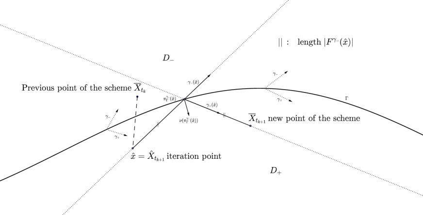
Figure 1: Correction of our scheme when the path crosses the boundary $\Gamma$.

Remark 4.4.

When the dimension $d$ is reduced to $1$ (one dimensional problem), the discontinuity surface reduces to a single point (say $0$). In this case and when the coefficient $a=a_{+}{\mathbb{I}}_{\mathnormal{y>0}}+a_{-}{\mathbb{I}}_{\mathnormal{y<0}}$ is constant on both sides of the discontinuity, it is remarkable that our Euler Scheme is exactly the same as the one described in [33].

Indeed, in this one-dimensional context, let $\varphi(y)=\left(a_{-}{\mathbb{I}}_{\mathnormal{y>0}}+a_{+}{\mathbb{I}}_{\mathnormal{y<0}}\right)y$. Note that $\varphi$ is a bijective map from $\mathbb{R}$ to $\mathbb{R}$. The Euler Scheme constructed in [33] is then defined by $\overline{X}_{0}=x_{0}$ and for all $k\in\{0,\dots,n\}$,

$$\overline{X}_{t_{k}}=\varphi^{-1}\left(\overline{Y}_{t_{k}}\right)$$

where $\overline{Y}_{0}=\varphi(x_{0})$ and for all $k\in\{0,\dots,n-1\}$

$$\overline{Y}_{t_{k+1}}=\overline{Y}_{t_{k}}+\left(a_{-}\sigma_{+}{\mathbb{I}}_{\mathnormal{\overline{Y}_{t_{k}}>0}}+a_{+}\sigma_{-}{\mathbb{I}}_{\mathnormal{\overline{Y}_{t_{k}}<0}}\right)(W_{t_{k+1}}-W_{t_{k}})\,;$$

(see [33] for details - please take care that [33] is written for the right-hand sided local time; the above computation is valid for the symmetric local time). For example if $\varphi(\overline{X}_{t_{k}})<0$ and $\overline{Y}_{t_{k+1}}\geq 0$, we get (because $\varphi^{-1}(0)=0$ and $\varphi^{-1}$ is continuous at $0$ and also because $\overline{X}$ and $\overline{Y}$ share the same sign),

$$\overline{X}_{t_{k+1}} =\varphi^{-1}\left(\varphi(\overline{X}_{t_{k}})+\left(a_{-}\sigma_{+}{\mathbb{I}}_{\mathnormal{\overline{Y}_{t_{k}}>0}}+a_{+}\sigma_{-}{\mathbb{I}}_{\mathnormal{\overline{Y}_{t_{k}}<0}}\right)\triangle W_{k}^{k+1}\right)$$

$$=\overline{X}_{t_{k}}+\int_{\varphi(\overline{X}_{t_{k}})}^{0}\left(\varphi^{-1}\right)^{\prime}(z)dz$$

$$\hskip 28.45274pt+\int_{0}^{\varphi(\overline{X}_{t_{k}})+(\underbrace{a_{-}\sigma_{+}{\mathbb{I}}_{\mathnormal{\overline{Y}_{t_{k}}>0}}}_{=0}+a_{+}\sigma_{-}{\mathbb{I}}_{\mathnormal{\overline{Y}_{t_{k}}<0}})\triangle W_{k}^{k+1}}\left(\varphi^{-1}\right)^{\prime}(z)dz$$

$$=\overline{X}_{t_{k}}-\varphi(\overline{X}_{t_{k}})\frac{1}{a_{+}}+\left(\varphi(\overline{X}_{t_{k}})+a_{+}\sigma_{-}\triangle W_{k}^{k+1}\right)\frac{1}{a_{-}}$$

$$=\frac{a_{+}}{a_{-}}\overline{X}_{t_{k}}+\frac{a_{+}}{a_{-}}\sigma_{-}\triangle W_{k}^{k+1},$$

which turns out to be the corresponding case in (4.9) in this one-dimensional context. This correspondence is valid in all cases and our transformed Euler Scheme may be viewed as some kind of generalization of the Euler Scheme presented in [33].

5 Convergence rate of our Euler scheme

The purpose of this section is to prove the following result.

Theorem 5.1.

Let $0<T<\infty$. Assume $(\mathbf{E})$. Let $m^{\prime}=\lceil 2+\frac{d}{4}\rceil+1$ and $k=m^{\prime}+2$. Assume that the coefficients $a_{ij}$ satisfy $(a_{\pm})_{ij}\in C_{b}^{2m^{\prime}-1}(\bar{D}_{\pm})$ and that $\Gamma$ is of class $C^{2m^{\prime}}$. Let $u_{0}:\mathbb{R}^{d}\to\mathbb{R}$ be in the space ${\cal D}(A^{k})$. Let $u$ be the classical solution of $(\mathcal{P}_{\mathrm{T}})$.

We have that for all $n$ large enough, and all $x_{0}$ in $\mathbb{R}^{d}$,

$$\Big{|}u(T,x_{0})-\mathbb{E}^{x_{0}}u_{0}(\overline{X}^{n}_{T})\Big{|}\leq K\sqrt{h_{n}},$$ (5.1)

where the constant $K$ depends on $d$, $\lambda$, $\Lambda$, $u_{0}$ and $T$.

Remark 5.2.

In this theorem the assumptions on $a(x)$ and $\Gamma$ involving the integers $m^{\prime}$ and $k$ are here in order to use Corollary 3.16, which ensures that we will have $\sup_{t\in[0,T],\,x\in\bar{D}_{\pm}}|\partial^{j}_{t}\partial^{\alpha}u_{\pm}(t,x)|<\infty$ for any $j\leq 2$ and any $|\alpha|\leq 4$. This control on the derivatives on $u$ is what we need in order to lead our convergence proof. In fact if there is a way to get this control under weaker assumptions on $a(x)$ and $\Gamma$, this will lead to a convergence theorem stated under these weaker assumptions.

5.1 Preliminary results

Lemma 5.3.

(see [3]) Consider an Itô process with uniformly bounded coefficients $dU_{t}=b_{t}dt+\sigma_{t}dW_{t}$ on $(\Omega,{\cal F},\mathbb{P}^{x_{0}})$. There exist some constants $c>0$ and $K$ (depending on $p\geq 1$, $T$ and the bounds on $\sigma$, $b$) such that, for any stopping times $S$ and $S^{\prime}$ (with $0\leq S\leq S^{\prime}\leq\delta\leq T$) and any $\eta\geq 0$,

$$\mathbb{P}^{x_{0}}\left[\sup_{t\in[S,S^{\prime}]}|U_{t}-U_{s}|\geq\eta\right] \leq K\exp\left(-c\frac{\eta^{2}}{\delta}\right)\leavevmode\nobreak\ ;$$ (5.2)

$$\mathbb{E}^{x_{0}}\left[\sup_{t\in[S,S^{\prime}]}|U_{t}-U_{s}|^{p}\right] \leq K\delta^{p/2}.$$ (5.3)

We have when $\overline{X}_{t_{k}}\in D_{+}$

$$\overline{X}_{t_{k+1}}=\hat{X}_{t_{k+1}}+\left[F^{\gamma_{+}}(\hat{X}_{t_{k+1}})\right]^{-}\left(\gamma_{+}(\pi^{\gamma_{+}}_{\Gamma}(\hat{X}_{t_{k+1}}))+\gamma_{-}(\pi^{\gamma_{+}}_{\Gamma}(\hat{X}_{t_{k+1}}))\right)$$

and when $X_{t_{k}}\in D_{-}$

$$\overline{X}_{t_{k+1}}=\hat{X}_{t_{k+1}}+\left[F^{\gamma_{-}}(\hat{X}_{t_{k+1}})\right]^{-}\left(\gamma_{+}(\pi^{\gamma_{-}}_{\Gamma}(\hat{X}_{t_{k+1}}))+\gamma_{-}(\pi^{\gamma_{-}}_{\Gamma}(\hat{X}_{t_{k+1}}))\right)$$

This shows that $(\overline{X}_{t})_{0\leq t\leq T}$ behaves like a continuous semimartingale on each of the intervals $[t_{k},t_{k+1})$. Using Tanaka’s formula, we have – for example for $\overline{X}_{t_{k}}\in D_{+}$ – that for any $t\in[t_{k},t_{k+1})$,

$$d\overline{X}_{t} =d\hat{X}_{t}+\frac{1}{2}\left(\gamma_{+}+\gamma_{-}\right)(\hat{X}_{t})dL_{t}^{0}(F^{\gamma_{+}}(\hat{X}))$$

$$\quad+\left[F^{\gamma_{+}}(\hat{X}_{t})\right]^{-}\Big{(}\nabla\left(\gamma_{+}+\gamma_{-}\right)(\hat{X}_{t})d\hat{X}_{t}$$

$$\hskip 85.35826pt+\frac{1}{2}{\rm Tr}\left[\mathbf{H}[\gamma_{+}+\gamma_{-}](\hat{X}_{t})a(\overline{X}_{t_{k})})\right]dt\Big{)}$$

$$\quad-{\mathbb{I}}_{\mathnormal{F^{\gamma_{+}}(\hat{X}_{t})<0}}\Big{[}\nabla\left(\gamma_{+}+\gamma_{-}\right)(\hat{X}_{t})a(\overline{X}_{t_{k}})\left(\nabla F^{\gamma_{+}}(\hat{X}_{t})\right)^{\ast}dt$$

$$\hskip 85.35826pt+\left(\gamma_{+}+\gamma_{-}\right)(\hat{X}_{t})\nabla F^{\gamma_{+}}(\hat{X}_{t})d\hat{X}_{t}\Big{]}$$

$$\quad\quad-{\mathbb{I}}_{\mathnormal{F^{\gamma_{+}}(\hat{X}_{t})<0}}\left(\gamma_{+}+\gamma_{-}\right)(\hat{X}_{t})\frac{1}{2}{\rm Tr}\left[\mathbf{H}[F^{\gamma_{+}}](\hat{X}_{t})a(\overline{X}_{t_{k}})\right]dt.$$ (5.4)

Lemma 5.4.

Under the assumptions of Theorem 5.1, for all $c>0$, there exists a constant $K(T)$ such that

$$h_{n}\;\mathbb{E}^{x_{0}}\sum_{i=0}^{n-1}\left[\exp\left(-c\frac{d^{2}(\overline{X}^{n}_{t_{i}},\Gamma)}{h_{n}}\right)\right]\leq K(T)\sqrt{h_{n}}.$$ (5.5)

Proof.

The idea is to use the occupation times formula. Using successively (4.3) and the inequality (4.7) of Proposition 4.3, we have $d\left(\overline{x},\Gamma\right)\geq\frac{1}{c_{2}}d\left(\hat{x},\Gamma\right)\geq\frac{1}{c_{1}c_{2}}|\tilde{F}^{\gamma_{\pm}}(\hat{x})|$ so that

$${\cal A}_{i+1} :=\mathbb{E}^{x_{0}}\left[\exp\left(-c\frac{d^{2}(\overline{X}^{n}_{t_{i+1}},\Gamma)}{h_{n}}\right)\right]$$

$$\leq\mathbb{E}^{x_{0}}\left[\exp\left(-c\frac{\left|\tilde{F}^{\gamma_{+}}(\hat{X}^{n}_{t_{i+1}})\right|^{2}}{|c_{1}c_{2}|^{2}h_{n}}\right){\mathbb{I}}_{\mathnormal{\overline{X}^{n}_{t_{i+1}}\in D_{-}}}\right]$$

$$\hskip 56.9055pt+\mathbb{E}^{x_{0}}\left[\exp\left(-c\frac{\left|\tilde{F}^{\gamma_{-}}(\hat{X}^{n}_{t_{i+1}})\right|^{2}}{|c_{1}c_{2}|^{2}h_{n}}\right){\mathbb{I}}_{\mathnormal{\overline{X}^{n}_{t_{i+1}}\in D_{+}}}\right]$$

$$\quad:={\cal A}_{i+1}^{+}+{\cal A}_{i+1}^{-}.$$ (5.6)

We concentrate on term ${\cal A}_{i+1}^{+}$ as both terms are treated in a similar manner.

Set $c^{\prime}=c/2c_{1}^{2}c_{2}^{2}>0$ and $g(x)=\exp(-2c^{\prime}x^{2}/h)$; it is easy to check that $|g(x)|+\sqrt{h}|g^{\prime}(x)|+h|g^{\prime\prime}(x)|\leq K(T)\exp(-c^{\prime}x^{2}/h)$. Hence, for $t\in[t_{i},t_{i+1}]$, Itô’s formula yields that

$$\mathbb{E}^{x_{0}}\exp\left(-2c^{\prime}\frac{\left|\tilde{F}^{\gamma_{+}}(\hat{X}^{n}_{t_{i+1}})\right|^{2}}{h_{n}}\right)$$

$$\leq K(T)\Big{[}\mathbb{E}^{x_{0}}\exp\big{(}-c^{\prime}\frac{\left|\tilde{F}^{\gamma_{+}}(\hat{X}^{n}_{t})\right|^{2}}{h_{n}}\big{)}$$

$$\hskip 56.9055pt+\frac{1}{h_{n}}\int_{t}^{t_{i+1}}\,ds\,\mathbb{E}^{x_{0}}\exp\big{(}-c^{\prime}\frac{\left|\tilde{F}^{\gamma_{+}}(\hat{X}^{n}_{s})\right|^{2}}{h_{n}}\big{)}\Big{]}.$$

We integrate this inequality with respect to $t$ over $[t_{i},t_{i+1}]$ to get

$$h_{n}\,{\cal A}^{+}_{i+1}\leq K(T)\int_{t_{i}}^{t_{i+1}}\,ds\,\mathbb{E}^{x_{0}}\exp\left(-c^{\prime}\frac{\left|\tilde{F}^{\gamma_{+}}(\hat{X}^{n}_{s})\right|^{2}}{h_{n}}\right).$$ (5.7)

(for possibly some new constant $K(T)$).

Observe that from (4.4),

$$d\langle\tilde{F}^{\gamma_{+}}(\hat{X}^{n}),\tilde{F}^{\gamma_{+}}(\hat{X}^{n})\rangle_{s} =\nabla\tilde{F}^{\gamma_{+}}(\hat{X}^{n}_{s})a(\overline{X}^{n}_{t_{i}})\left[\nabla\tilde{F}^{\gamma_{+}}(\hat{X}^{n}_{s})\right]^{\ast}\,ds\geq\lambda ds.$$ (5.8)

Indeed, using the Cauchy-Schwarz inequality and $|\nu(\hat{x})|=1$, we have that

$$\nabla\tilde{F}^{\gamma_{+}}(\hat{x})a(\overline{x})\left[\nabla\tilde{F}^{\gamma_{+}}(\hat{x})\right]^{\ast} =\frac{\nu^{\ast}(\hat{x})a(\overline{x})\nu(\hat{x})}{\langle\nu(\hat{x}),\tilde{\gamma}_{+}(\hat{x})\rangle^{2}}=\frac{\langle\nu(\hat{x}),a(\overline{x})\nu(\hat{x})\rangle}{\langle\nu(\hat{x}),\frac{a(\hat{x})\nu(\hat{x})}{|a(\hat{x})\nu(\hat{x})|}\rangle^{2}}$$

$$\geq\frac{\langle\nu(\hat{x}),a(\overline{x})\nu(\hat{x})\rangle}{|\nu(\hat{x})|^{2}|a(\hat{x})\nu(\hat{x})|^{2}}|a(\hat{x})\nu(\hat{x})|^{2}=\langle\nu(\hat{x}),a(\overline{x})\nu(\hat{x})\rangle$$

$$\geq\lambda$$

which justifies (5.8).

It readily follows from the occupation times formula that

$$h_{n}\,{\cal A}^{+}_{i+1}\leq K(T)\int_{-R}^{R}dy\exp\left(-c^{\prime}\frac{y^{2}}{h_{n}}\right)\mathbb{E}^{x_{0}}\left[\triangle_{i}^{i+1}L^{y}\left(\tilde{F}^{\gamma_{+}}(\hat{X}^{n}_{.})\right)\right].$$ (5.9)

Now,

$$\mathbb{E}^{x_{0}}\left[L^{y}_{t_{i+1}}\left(\tilde{F}^{\gamma_{+}}(\hat{X}^{n}_{.})\right)-L^{y}_{t_{i}}\left(\tilde{F}^{\gamma_{+}}(\hat{X}^{n}_{.})\right)\right]$$

$$=2\mathbb{E}^{x_{0}}\Big{[}\left(\tilde{F}^{\gamma_{+}}(\hat{X}^{n}_{t_{i+1}})-y\right)^{+}-\left(\tilde{F}^{\gamma_{+}}(\hat{X}^{n}_{t_{i}})-y\right)^{+}$$

$$\hskip 85.35826pt-\int_{t_{i}}^{t_{i+1}}{\mathbb{I}}_{\mathnormal{\tilde{F}^{\gamma_{+}}(\hat{X}^{n}_{s})\geq y}}d\left(\tilde{F}^{\gamma_{+}}(\hat{X}^{n}_{s})\right)\Big{]}$$

$$\leq 2\mathbb{E}^{x_{0}}\left[\left(\tilde{F}^{\gamma_{+}}(\hat{X}^{n}_{t_{i+1}})-y\right)^{+}-\left(\tilde{F}^{\gamma_{+}}(\hat{X}^{n}_{t_{i}})-y\right)^{+}\right]+K(T)h_{n}.$$

Therefore, $\sum_{i=0}^{n-1}\mathbb{E}^{x_{0}}\left[L^{y}_{t_{i+1}}\left(\tilde{F}^{\gamma_{+}}(\hat{X}^{n}_{.})\right)-L^{y}_{t_{i}}\left(\tilde{F}^{\gamma_{+}}(\hat{X}^{n}_{.})\right)\right]\leq K(T)$ uniformly in $|y|\leq R$ since the sum is telescoping. We can thus conclude that $h_{n}\sum_{i=0}^{n-1}{\cal A}^{+}_{i+1}\leq K(T)\sqrt{h_{n}}$.

The sum $h_{n}\sum_{i=0}^{n-1}{\cal A}^{-}_{i+1}$ is treated similarly. The proof of the Lemma is complete. ∎

5.2 Error decomposition

In all the sequel $x_{0}$ is arbitrarily fixed.

For all $0\leq k\leq n$ set

$$\theta^{n}_{k}:=T-t^{n}_{k}.$$

The proof of Theorem 5.1 proceeds as follows (we omit the superscript $n$). Since $u(0,x)=u_{0}(x)$ for all $x\in\mathbb{R}^{d}$ and $u(T,x_{0})=\mathbb{E}^{x_{0}}u(T,\overline{X}_{0})$, the discretization error at time $T$ can be decomposed as follows:

$$\begin{split}\epsilon^{x_{0}}_{T}&=\left|u(T,x_{0})-\mathbb{E}^{x_{0}}u_{0}\left(\overline{X}_{T}\right)\right|\\ &=\Big{|}\sum_{k=0}^{n-1}\mathbb{E}^{x_{0}}u(T-t_{k},\overline{X}_{t_{k}})-\mathbb{E}^{x_{0}}u(T-t_{k+1},\overline{X}_{t_{k+1}})\Big{|},\end{split}$$ (5.10)

and thus

$$\begin{split}\epsilon^{x_{0}}_{T}&\leq\Big{|}\sum_{k=0}^{n-1}\mathbb{E}^{x_{0}}\left\{u(\theta_{k},\overline{X}_{t_{k}})-u(\theta_{k+1},\overline{X}_{t_{k}})\right.\\ &\quad\quad\quad\quad\left.+u(\theta_{k+1},\overline{X}_{t_{k}})-u(\theta_{k+1},\overline{X}_{t_{k+1}})\right\}\Big{|}.\\ \end{split}$$ (5.11)

The rest of this section is devoted to the analysis of

$$\left|\sum_{k=0}^{n-1}\mathbb{E}^{x_{0}}(T_{k}-S_{k})\right|,$$

where the time increment $T_{k}$ is defined as

$$T_{k}:=u(\theta_{k},\overline{X}_{t_{k}})-u(\theta_{k+1},\overline{X}_{t_{k}})$$ (5.12)

and the space increment is defined as

$$S_{k}:=u(\theta_{k+1},\overline{X}_{t_{k+1}})-u(\theta_{k+1},\overline{X}_{t_{k}}).$$ (5.13)

5.3 Estimate for the time increment $T_{k}$

Remember the definition (5.12) of $T_{k}$ and that $\theta_{k}=T-t_{k}$. We have

$$\begin{split}&\left\{u(\theta_{k},\overline{X}_{t_{k}})-u(\theta_{k+1},\overline{X}_{t_{k}})\right\}{\mathbb{I}}_{\mathnormal{\overline{X}_{t_{k}}\in D_{+}}}\\ &\quad=h_{n}\partial_{t}u(\theta_{k+1},\overline{Y}_{t_{k}}){\mathbb{I}}_{\mathnormal{\overline{X}_{t_{k}}\in D_{+}}}\\ &\hskip 56.9055pt+h_{n}^{2}\int_{[0,1]^{2}}\partial^{2}_{tt}u(\theta_{k+1}+\alpha_{1}\alpha_{2}h_{n},\overline{X}_{t_{k}})\alpha_{1}\leavevmode\nobreak\ d\alpha_{1}d\alpha_{2}\leavevmode\nobreak\ {\mathbb{I}}_{\mathnormal{\overline{X}_{t_{k}}\in D_{+}}}\\ &\quad=:T_{k}^{+}+R_{k}^{+}.\end{split}$$

Similarly,

$$\begin{split}&\left\{u(\theta_{k},\overline{X}_{t_{k}})-u(\theta_{k+1},\overline{X}_{t_{k}})\right\}{\mathbb{I}}_{\mathnormal{\overline{X}_{t_{k}}\in D_{-}}}\\ &\quad=h_{n}\partial_{t}u(\theta_{k+1},\overline{X}_{t_{k}}){\mathbb{I}}_{\mathnormal{\overline{X}_{t_{k}}\in D_{-}}}\\ &\hskip 56.9055pt+h_{n}^{2}\int_{[0,1]^{2}}\partial^{2}_{tt}u(\theta_{k+1}+\alpha_{1}\alpha_{2}h_{n},\overline{X}_{t_{k}})\alpha_{1}\leavevmode\nobreak\ d\alpha_{1}d\alpha_{2}\leavevmode\nobreak\ {\mathbb{I}}_{\mathnormal{\overline{X}_{t_{k}}\in D_{-}}}\\ &\quad=:T_{k}^{-}+R_{k}^{-}.\end{split}$$

In view of Corollary 3.16 and Remark 5.2 we have

$$\mathbb{E}^{x_{0}}|R_{k}^{+}+R_{k}^{-}|\leq C\,h_{n}^{2}.$$

From the preceding we deduce

$$\mathbb{E}^{x_{0}}T_{k}=\mathbb{E}^{x_{0}}\partial_{t}u(\theta_{k+1},\overline{X}_{t_{k}})h_{n}+O(h_{n}^{2}).$$ (5.14)

5.4 Expansion of the space increment $S_{k}$

Let $S_{k}$ be defined as in (5.13). Set

$$\triangle_{k+1}\overline{X} :=\overline{X}_{t_{k+1}}-\overline{X}_{t_{k}}$$

$$\triangle^{\sharp}_{k+1}\overline{X} :=\hat{X}_{t_{k+1}}-\overline{X}_{t_{k}}.$$

and recall that $\triangle_{k+1}W=W_{t_{k+1}}-W_{t_{k}}$.

Proposition 5.5.

$$\mathbb{E}^{x_{0}}|(\triangle^{\sharp}_{k+1}\overline{X})^{\alpha}|\leq C(\alpha)h_{n}^{|\alpha|/2}.$$ (5.15)

Proof.

This is a consequence of the result of Lemma 5.3 combined with the fact that $|(x)^{\alpha}|\leq|x|^{|\alpha|}$ for any $x\in\mathbb{R}^{d}$. ∎

We emphasize that, due to the definition of our stochastic scheme, $\triangle^{\sharp}_{k+1}\overline{X}$ does not coincide with $\overline{X}_{t_{k+1}}-\overline{X}_{t_{k}}$ when $\overline{X}_{t_{k+1}}$ and $\overline{X}_{t_{k}}$ do not belong to the same region, which explains the two notations $\triangle$ and $\triangle^{\sharp}$.

We need to introduce the four following events:

$$\begin{cases}\Omega_{k}^{++}&:=[\overline{X}_{t_{k}}\in\overline{D}_{+}\leavevmode\nobreak\ \text{and}\leavevmode\nobreak\ \hat{X}_{t_{k+1}}\in D_{+}],\\ \Omega_{k}^{--}&:=[\overline{X}_{t_{k}}\in D_{-}\leavevmode\nobreak\ \text{and}\leavevmode\nobreak\ \hat{X}_{t_{k+1}}\in\overline{D}_{-}],\\ \Omega_{k}^{+-}&:=[\overline{X}_{t_{k}}\in D_{+}\leavevmode\nobreak\ \text{and}\leavevmode\nobreak\ \hat{X}_{t_{k+1}}\in\overline{D}_{-}],\\ \Omega_{k}^{-+}&:=[\overline{X}_{t_{k}}\in\overline{D}_{-}\leavevmode\nobreak\ \text{and}\leavevmode\nobreak\ \hat{X}_{t_{k+1}}\in D_{+}].\end{cases}$$ (5.16)

In view of the definition of our stochastic numerical scheme we have

$$\text{On}\leavevmode\nobreak\ \Omega_{k}^{++},\leavevmode\nobreak\ \triangle_{k+1}\overline{X}=\triangle^{\sharp}_{k+1}\overline{X}.$$

Therefore

$$\begin{split}S_{k}{\mathbb{I}}_{\mathnormal{\Omega_{k}^{++}}}&=\langle\triangle_{k+1}\overline{X},\nabla_{x}u(\theta_{k+1},\overline{X}_{t_{k}})\rangle\leavevmode\nobreak\ {\mathbb{I}}_{\mathnormal{\Omega_{k}^{++}}}\\ &+\dfrac{1}{2}\left(\triangle_{k+1}\overline{X}\right)^{\ast}{\rm\bf H}[u](\theta_{k+1},\overline{X}_{t_{k}})\triangle_{k+1}\overline{X}\leavevmode\nobreak\ {\mathbb{I}}_{\mathnormal{\Omega_{k}^{++}}}\\ &\quad+\sum_{|{\alpha}|=3}\frac{1}{\alpha!}(\triangle_{k+1}\overline{X})^{\alpha}\frac{\partial^{3}u}{\partial x^{\alpha}}(\theta_{k+1},\overline{X}_{t_{k}})\leavevmode\nobreak\ {\mathbb{I}}_{\mathnormal{\Omega_{k}^{++}}}\\ &\quad+\int_{0}^{1}d\xi\sum_{|{\alpha}|=4}\frac{(1-\xi)^{4}}{\alpha!}(\triangle_{k+1}\overline{X})^{\alpha}\frac{\partial^{4}u}{\partial x^{\alpha}}(\theta_{k+1},\overline{X}_{t_{k}}+\xi\triangle_{k+1}\overline{X})\leavevmode\nobreak\ {\mathbb{I}}_{\mathnormal{\Omega_{k}^{++}}}\\ &=:S_{k}^{++1}+S_{k}^{++2}+S_{k}^{++3}+S_{k}^{++4}.\end{split}$$

Similarly,

$$\begin{split}S_{k}{\mathbb{I}}_{\mathnormal{\Omega_{k}^{--}}}&=\langle\triangle_{k+1}\overline{X},\nabla_{x}u(\theta_{k+1},\overline{X}_{t_{k}})\rangle\leavevmode\nobreak\ {\mathbb{I}}_{\mathnormal{\Omega_{k}^{--}}}\\ &+\dfrac{1}{2}\left(\triangle_{k+1}\overline{X}\right)^{\ast}{\rm\bf H}[u](\theta_{k+1},\overline{X}_{t_{k}})\triangle_{k+1}\overline{X}\leavevmode\nobreak\ {\mathbb{I}}_{\mathnormal{\Omega_{k}^{--}}}\\ &\quad+\sum_{|{\alpha}|=3}\frac{1}{\alpha!}(\triangle_{k+1}\overline{X})^{\alpha}\frac{\partial^{3}u}{\partial x^{\alpha}}(\theta_{k+1},\overline{X}_{t_{k}})\leavevmode\nobreak\ {\mathbb{I}}_{\mathnormal{\Omega_{k}^{--}}}\\ &\quad+\int_{0}^{1}d\xi\sum_{|{\alpha}|=4}\frac{(1-\xi)^{4}}{\alpha!}(\triangle_{k+1}\overline{X})^{\alpha}\frac{\partial^{4}u}{\partial x^{\alpha}}(\theta_{k+1},\overline{X}_{t_{k}}+\xi\triangle_{k+1}\overline{X})\leavevmode\nobreak\ {\mathbb{I}}_{\mathnormal{\Omega_{k}^{--}}}\\ &=:S_{k}^{--1}+S_{k}^{--2}+S_{k}^{--3}+S_{k}^{--4}.\end{split}$$

We now use that $\Omega_{k}^{++}\cup\Omega_{k}^{--}=\Omega-(\Omega_{k}^{+-}\cup\Omega_{k}^{-+})$. Notice that $\Omega_{k}^{+-}\cup\Omega_{k}^{-+}$ belongs to the $\sigma$-field generated by $(W_{t})$ up to time $t_{k+1}$. In view of the first line of (4.9) and the fact that ${\mathbb{E}}^{{\cal F}_{t_{k}}}\Delta W_{k+1}=0$, we get

$$\begin{split}\mathbb{E}^{x_{0}}(S_{k}^{++1}+S_{k}^{--1})&=\frac{h_{n}}{2}\mathbb{E}^{x_{0}}\left[\langle\partial a(\overline{X}_{t_{k}}),\nabla_{x}u(\theta_{k+1},\overline{X}_{t_{k}})\rangle\right]\\ &\quad-\mathbb{E}^{x_{0}}\left[\langle\triangle^{\sharp}_{k+1}\overline{X},\nabla_{x}u(\theta_{k+1},\overline{X}_{t_{k}})\rangle\leavevmode\nobreak\ {\mathbb{I}}_{\mathnormal{\Omega_{k}^{+-}\cup\Omega_{k}^{-+}}}\right].\\ &\quad\end{split}$$

Proceeding similarly and conditioning $(\triangle^{\sharp}_{k+1}\overline{X})^{2}$ w.r.t. the past of $(W_{t})$ up to time $t_{k}$, we obtain

$$\begin{split}\mathbb{E}^{x_{0}}(S_{k}^{++2}+S_{k}^{--2})&=\dfrac{1}{2}\mathbb{E}^{x_{0}}\left[{\rm Tr}[\sigma{\bf H}[u]\sigma^{\ast}](\theta_{k+1},\overline{X}_{t_{k}})\right]h_{n}\\ &\quad-\dfrac{1}{2}\mathbb{E}^{x_{0}}\left[(\triangle^{\sharp}_{k+1}\overline{X})^{\ast}{\bf H}[u](\theta_{k+1},\overline{X}_{t_{k}})\triangle^{\sharp}_{k+1}\overline{X}\leavevmode\nobreak\ {\mathbb{I}}_{\mathnormal{\Omega_{k}^{+-}\cup\Omega_{k}^{-+}}}\right]\end{split}$$

and since $\mathbb{E}^{x_{0}}(\triangle_{k+1}W)^{\alpha}=0$ whenever $|\alpha|=3$,

$$\begin{split}\mathbb{E}^{x_{0}}(S_{k}^{++3}+S_{k}^{--3})&=\sum_{|{\alpha}|=3}\frac{1}{\alpha!}\mathbb{E}^{x_{0}}\left[(\triangle^{\sharp}_{k+1}\overline{X})^{\alpha}\frac{\partial^{3}u}{\partial x^{\alpha}}(\theta_{k+1},\overline{X}_{t_{k}})\right]\\ &\quad-\sum_{|{\alpha}|=3}\frac{1}{\alpha!}\mathbb{E}^{x_{0}}\left[(\triangle^{\sharp}_{k+1}\overline{X})^{\alpha}\frac{\partial^{3}u}{\partial x^{\alpha}}(\theta_{k+1},\overline{X}_{t_{k}})\leavevmode\nobreak\ {\mathbb{I}}_{\mathnormal{\Omega_{k}^{+-}\cup\Omega_{k}^{-+}}}\right].\end{split}$$

We have, combining the results of Corollary 3.16 and Proposition 5.5,

$$\left|\sum_{|{\alpha}|=3}\frac{1}{\alpha!}\mathbb{E}^{x_{0}}\left[(\triangle^{\sharp}_{k+1}\overline{X})^{\alpha}\frac{\partial^{3}u}{\partial x^{\alpha}}(\theta_{k+1},\overline{X}_{t_{k}})\right]\right|\leq C\;h_{n}^{3/2}.$$ (5.17)

In addition, and for the same reasons, we have

$$\mathbb{E}^{x_{0}}|S_{k}^{++4}+S_{k}^{--4}|\leq C\,h_{n}^{2}.$$

To summarize the calculations of this subsection, we have obtained

$$\begin{split}&\mathbb{E}^{x_{0}}S_{k}=\\ &\mathbb{E}^{x_{0}}\mathcal{L}u(\theta_{k+1},\overline{X}_{t_{k}})h_{n}+\mathbb{E}^{x_{0}}\left[\left(S_{k}-\langle\triangle^{\sharp}_{k+1}\overline{X},\nabla_{x}u(\theta_{k+1},\overline{X}_{t_{k}})\rangle\right)\leavevmode\nobreak\ {\mathbb{I}}_{\mathnormal{\Omega_{k}^{+-}\cup\Omega_{k}^{-+}}}\right]\\ &\!\!\!-\mathbb{E}^{x_{0}}\Big{[}\Big{(}\dfrac{1}{2}(\triangle^{\sharp}_{k+1}\overline{X})^{\ast}{\bf H}[u](\theta_{k+1},\overline{X}_{t_{k}})\triangle^{\sharp}_{k+1}\overline{X}\\ &+\sum_{|{\alpha}|=3}\frac{1}{\alpha!}(\triangle^{\sharp}_{k+1}\overline{X})^{\alpha}\frac{\partial^{3}u}{\partial x^{\alpha}}(\theta_{k+1},\overline{X}_{t_{k}})\Big{)}\leavevmode\nobreak\ {\mathbb{I}}_{\mathnormal{\Omega_{k}^{+-}\cup\Omega_{k}^{-+}}}\Big{]}+O(h_{n}^{3/2})\\ &=:\mathbb{E}^{x_{0}}\mathcal{L}u(\theta_{k+1},\overline{X}_{t_{k}})h_{n}+{\mathbb{E}}^{x_{0}}\mathcal{R}^{(1)}_{k}-\mathbb{E}^{x_{0}}\mathcal{R}^{(2)}_{k}+O(h_{n}^{3/2}).\end{split}$$ (5.18)

We now estimate the remaining terms $\mathbb{E}^{x_{0}}\mathcal{R}^{(1)}_{k}$ and $\mathbb{E}^{x_{0}}\mathcal{R}^{(2)}_{k}$.

5.5 Control of the term $\mathbb{E}^{x_{0}}\mathcal{R}^{(1)}_{k}$. Expansion around a well chosen point in $\Gamma$

On the event $\Omega_{k}^{+-}$ we have that $\overline{X}_{t_{k+1}}$ and $\overline{X}_{t_{k}}$ are close to $\Gamma$. On this event, we also have that $\hat{X}_{t_{k+1}}\in D_{-}$ and $\overline{X}_{t_{k}}\in D_{+}$. Remember our definition of $(F^{\gamma_{+}}(x),\pi_{\Gamma}^{\gamma_{+}}(x))$ for $x\in D_{-}$.

5.5.1 Decomposition of $\mathbb{E}^{x_{0}}\mathcal{R}^{(1)}_{k}$

As the function $u$ is continuous across the surface $\Gamma$ at point $\pi_{\Gamma}^{\gamma_{+}}(x)$, we get

$$\begin{split}&\mathbb{E}^{x_{0}}\left(\left(S_{k}-\langle\triangle^{\sharp}_{k+1}\overline{X},\nabla_{x}u(\theta_{k+1},\overline{X}_{t_{k}})\rangle\right)\leavevmode\nobreak\ {\mathbb{I}}_{\mathnormal{\Omega_{k}^{+-}}}\right]\\ &=\mathbb{E}^{x_{0}}\big{[}\big{(}\big{(}u(\theta_{k+1},\overline{X}_{t_{k+1}})-u(\theta_{k+1},\pi_{\Gamma}^{\gamma_{+}}(\hat{X}_{t_{k+1}}))\big{)}\\ &\;\;+\left(u(\theta_{k+1},\pi_{\Gamma}^{\gamma_{+}}(\hat{X}_{t_{k+1}}))-u(\theta_{k+1},\overline{X}_{t_{k}})\right)\big{)}\leavevmode\nobreak\ {\mathbb{I}}_{\mathnormal{\Omega_{k}^{+-}}}\big{]}\\ &\quad\quad-\mathbb{E}^{x_{0}}\left[\langle\triangle^{\sharp}_{k+1}\overline{X},\nabla_{x}u_{+}(\theta_{k+1},\pi_{\Gamma}^{\gamma_{+}}(\hat{X}_{t_{k+1}}))\rangle\leavevmode\nobreak\ {\mathbb{I}}_{\mathnormal{\Omega_{k}^{+-}}}\right]\\ &\quad\quad-\mathbb{E}^{x_{0}}\left[\langle\triangle^{\sharp}_{k+1}\overline{X},\nabla_{x}u(\theta_{k+1},\overline{X}_{t_{k}})-\nabla_{x}u_{+}(\theta_{k+1},\pi_{\Gamma}^{\gamma_{+}}(\hat{X}_{t_{k+1}}))\rangle\leavevmode\nobreak\ {\mathbb{I}}_{\mathnormal{\Omega_{k}^{+-}}}\right]\end{split}$$

so that

$$\begin{split}&\mathbb{E}^{x_{0}}\left(\left(S_{k}-\langle\triangle^{\sharp}_{k+1}\overline{X},\nabla_{x}u(\theta_{k+1},\overline{X}_{t_{k}})\rangle\right)\leavevmode\nobreak\ {\mathbb{I}}_{\mathnormal{\Omega_{k}^{+-}}}\right]\\ =&\left\{\mathbb{E}^{x_{0}}\left[\langle\overline{X}_{t_{k+1}}-\pi_{\Gamma}^{\gamma_{+}}(\hat{X}_{t_{k+1}}),\nabla_{x}u_{-}(\theta_{k+1},\pi_{\Gamma}^{\gamma_{+}}(\hat{X}_{t_{k+1}}))\rangle{\mathbb{I}}_{\mathnormal{\Omega_{k}^{+-}}}\right]\right.\\ &\quad\quad-\mathbb{E}^{x_{0}}\left[\langle\overline{X}_{t_{k}}-\pi_{\Gamma}^{\gamma_{+}}(\hat{X}_{t_{k+1}}),\nabla_{x}u_{+}(\theta_{k+1},\pi_{\Gamma}^{\gamma_{+}}(\hat{X}_{t_{k+1}}))\rangle\leavevmode\nobreak\ {\mathbb{I}}_{\mathnormal{\Omega_{k}^{+-}}}\right]\\ &\quad\quad\left.-\mathbb{E}^{x_{0}}\left[\langle\triangle^{\sharp}_{k+1}\overline{X},\nabla_{x}u_{+}(\theta_{k+1},\pi_{\Gamma}^{\gamma_{+}}(\hat{X}_{t_{k+1}}))\rangle\leavevmode\nobreak\ {\mathbb{I}}_{\mathnormal{\Omega_{k}^{+-}}}\right]\right\}_{:=L_{k}^{+-1}}\\ &\quad\quad+\left\{\int_{0}^{1}d\xi\sum_{|{\alpha}|=2}\frac{(1-\xi)^{2}}{\alpha!}\mathbb{E}^{x_{0}}\left[(\hat{X}_{t_{k+1}}-\pi_{\Gamma}^{\gamma_{+}}(\hat{X}_{t_{k+1}}))^{\alpha}\right.\right.\\ &\quad\quad\quad\quad\left.\times\frac{\partial^{\alpha}u}{\partial x^{\alpha}}(\theta_{k+1},\pi_{\Gamma}^{\gamma_{+}}(\hat{X}_{t_{k+1}})+\xi(\hat{X}_{t_{k+1}}-\pi_{\Gamma}^{\gamma_{+}}(\hat{X}_{t_{k+1}})))\leavevmode\nobreak\ {\mathbb{I}}_{\mathnormal{\Omega_{k}^{+-}}}\right]\\ &\quad\quad\quad-\int_{0}^{1}d\xi\sum_{|{\alpha}|=2}\frac{(1-\xi)^{2}}{\alpha!}\mathbb{E}^{x_{0}}\left[(\overline{X}_{t_{k}}-\pi_{\Gamma}^{\gamma_{+}}(\hat{X}_{t_{k+1}}))^{\alpha}\right.\\ &\quad\quad\quad\quad\left.\left.\times\frac{\partial^{\alpha}u}{\partial x^{\alpha}}(\theta_{k+1},\pi_{\Gamma}^{\gamma_{+}}(\hat{X}_{t_{k+1}})+\xi(\overline{X}_{t_{k}}-\pi_{\Gamma}^{\gamma_{+}}(\hat{X}_{t_{k+1}})))\leavevmode\nobreak\ {\mathbb{I}}_{\mathnormal{\Omega_{k}^{+-}}}\right]\right\}_{:=L_{k}^{+-2}}\\ &-\left\{\mathbb{E}^{x_{0}}\left[\langle\triangle^{\sharp}_{k+1}\overline{X},\nabla_{x}u_{+}(\theta_{k+1},\overline{X}_{t_{k}})-\nabla_{x}u_{+}(\theta_{k+1},\pi_{\Gamma}^{\gamma_{+}}(\hat{X}_{t_{k+1}}))\rangle\leavevmode\nobreak\ {\mathbb{I}}_{\mathnormal{\Omega_{k}^{+-}}}\right]\right\}_{:=L_{k}^{+-3}}\\ =&L_{k}^{+-1}+L_{k}^{+-2}+L_{k}^{+-3}.\end{split}$$

5.5.2 Canceling the term $L_{k}^{+-1}$ using the transmission condition

Observe that due to the fact that

$$\left(\hat{X}_{t_{k}}-\pi_{\Gamma}^{\gamma_{+}}(\hat{X}_{t_{k+1}})\right)+\left(\hat{X}_{t_{k+1}}-\hat{X}_{t_{k}}\right)=\hat{X}_{t_{k+1}}-\pi_{\Gamma}^{\gamma_{+}}(\hat{X}_{t_{k+1}}).$$

we have that

$$\begin{split}L_{k}^{+-1}&=\mathbb{E}^{x_{0}}\left[\left(\langle\overline{X}_{t_{k+1}}-\pi_{\Gamma}^{\gamma_{+}}(\hat{X}_{t_{k+1}}),\nabla_{x}u_{-}(\theta_{k+1},\pi_{\Gamma}^{\gamma_{+}}(\hat{X}_{t_{k+1}}))\rangle\right.\right.\\ &\quad\quad\quad\quad\left.\left.-\langle\hat{X}_{t_{k+1}}-\pi_{\Gamma}^{\gamma_{+}}(\hat{X}_{t_{k+1}}),\nabla_{x}u_{+}(\theta_{k+1},\pi_{\Gamma}^{\gamma_{+}}(\hat{X}_{t_{k+1}}))\rangle\right)\leavevmode\nobreak\ {\mathbb{I}}_{\mathnormal{\Omega_{k}^{+-}}}\right]\\ &=\mathbb{E}^{x_{0}}\left[F^{\gamma_{+}}(\hat{X}_{t_{k+1}})\left(\langle-\gamma_{-}(\pi_{\Gamma}^{\gamma_{+}}(\hat{X}_{t_{k+1}})),\nabla_{x}u_{-}(\theta_{k+1},\pi_{\Gamma}^{\gamma_{+}}(\hat{X}_{t_{k+1}}))\rangle\right.\right.\\ &\quad\quad\quad\quad\quad\quad\left.\left.-\langle\gamma_{+}(\pi_{\Gamma}^{\gamma_{+}}(\hat{X}_{t_{k+1}})),\nabla_{x}u_{+}(\theta_{k+1},\pi_{\Gamma}^{\gamma_{+}}(\hat{X}_{t_{k+1}}))\rangle\right)\leavevmode\nobreak\ {\mathbb{I}}_{\mathnormal{\Omega_{k}^{+-}}}\right]\\ &=0,\end{split}$$

where we have used the vector problem solved by $(F^{\gamma_{+}},\pi_{\Gamma}^{\gamma_{+}})$ and Equation (4.5) (i.e. the transmission condition $(\star)$ and the definition of $\gamma_{\pm}(x)$).

5.5.3 The term $L_{k}^{+-2}$

We now turn to the term $L_{k}^{+-2}$.

The term $L_{k}^{+-2}$ is the sum of two terms. These two terms are treated similarly, so we concentrate only on the first. Let $\alpha$ such that $|\alpha|=2$. We have that

$$\begin{split}\mathbb{E}^{x_{0}}\left[\left|(\overline{X}_{t_{k}}-\pi_{\Gamma}^{\gamma_{+}}(\hat{X}_{t_{k+1}}))^{\alpha}\right|\leavevmode\nobreak\ {\mathbb{I}}_{\mathnormal{\Omega_{k}^{+-}}}\right]&\leq c_{1}\mathbb{E}^{x_{0}}\left[|\overline{X}_{t_{k}}-\pi_{\Gamma}^{\gamma_{+}}(\hat{X}_{t_{k+1}})|^{2}\leavevmode\nobreak\ {\mathbb{I}}_{\mathnormal{\Omega_{k}^{+-}}}\right]\\ &\leq c_{2}\mathbb{E}^{x_{0}}\left[|\triangle^{\sharp}_{k+1}X|^{2}\leavevmode\nobreak\ {\mathbb{I}}_{\mathnormal{\Omega_{k}^{+-}}}\right].\end{split}$$

The same kind of treatment can be performed for the second term of $L_{k}^{+-2}$. Conditionning w.r.t ${\cal F}_{t_{k}}$ and applying the Cauchy-Schwarz inequality in the conditionnal expectation, we find using the result of Lemma 5.3,

$$\begin{split}|L_{k}^{+-2}|&\leq C\mathbb{E}^{x_{0}}\left[{\mathbb{E}}^{{\cal F}_{t_{k}}}\left[\big{|}\triangle^{\sharp}_{k+1}X\big{|}^{4}\right]^{1/2}\leavevmode\nobreak\ {\mathbb{P}}^{{\cal F}_{t_{k}}}\left(\Omega_{k}^{+-}\right)^{1/2}\right]\\ &\leq C\,h_{n}\leavevmode\nobreak\ {\mathbb{E}}^{x_{0}}{\mathbb{P}}^{{\cal F}_{t_{k}}}\left(\Omega_{k}^{+-}\right)^{1/2}.\end{split}$$

5.5.4 The term $L_{k}^{+-3}$

For the term $L_{k}^{+-3}$, we may perform a Taylor’s expansion to the term

$$\nabla_{x}u_{+}(\theta_{k+1},\overline{X}_{t_{k}})-\nabla_{x}u_{+}(\theta_{k+1},\pi_{\Gamma}^{\gamma_{+}}(\hat{X}_{t_{k+1}})).$$

Using Corollary 3.16 and the Cauchy-Schwarz inequality, we find that

$$|L_{k}^{+-3}| \leq C\mathbb{E}^{x_{0}}\left[\big{|}\triangle^{\sharp}_{k+1}\overline{X}\big{|}\big{|}\overline{X}_{t_{k}}-\pi_{\Gamma}^{\gamma_{+}}(\hat{X}_{t_{k+1}})\rangle\big{|}\leavevmode\nobreak\ {\mathbb{I}}_{\mathnormal{\Omega_{k}^{+-}}}\right]$$

$$\leq C\mathbb{E}^{x_{0}}\left[\big{|}\triangle^{\sharp}_{k+1}X\big{|}^{2}\leavevmode\nobreak\ {\mathbb{I}}_{\mathnormal{\Omega_{k}^{+-}}}\right].$$ (5.19)

Finally, as for the term $L_{k}^{+-2}$, we find that

$$\begin{split}|L_{k}^{+-3}|\leq C\,h_{n}{\mathbb{E}}^{x_{0}}{\mathbb{P}}^{{\cal F}_{t_{k}}}\left(\Omega_{k}^{+-}\right)^{1/2}.\end{split}$$

Using the same method for the other side $\Omega_{k}^{-+}$, we find that

$$\begin{split}\mathbb{E}^{x_{0}}{\cal R}_{k}^{(1)}\leq C\,h_{n}{\mathbb{E}}^{x_{0}}\left({\mathbb{P}}^{{\cal F}_{t_{k}}}\left(\Omega_{k}^{+-}\right)^{1/2}+{\mathbb{P}}^{{\cal F}_{t_{k}}}\left(\Omega_{k}^{-+}\right)^{1/2}\right).\end{split}$$

5.6 Summing up

The term $\mathbb{E}^{x_{0}}\mathcal{R}^{(2)}_{k}$ can be estimated using the same techniques used in the previous section and we omit the details.

Using now the fact that $\partial_{t}u-{\cal L}u=0$, we finally find that

$$\epsilon^{x_{0}}_{T}\leq C\,h_{n}\,{\mathbb{E}}^{x_{0}}\sum_{k=0}^{n-1}\left({\mathbb{P}}^{{\cal F}_{t_{k}}}\left(\Omega_{k}^{+-}\right)^{1/2}+{\mathbb{P}}^{{\cal F}_{t_{k}}}\left(\Omega_{k}^{-+}\right)^{1/2}\right)+C\sqrt{h_{n}}.$$ (5.20)

Observe – using the result of Lemma 5.3 – that

$${\mathbb{P}}^{{\cal F}_{t_{k}}}\left(\Omega_{k}^{+-}\right)^{1/2} ={\mathbb{P}}^{{\cal F}_{t_{k}}}\left(\overline{X}_{t_{k}}\in D_{+},\hat{X}_{t_{k+1}}\in D_{-}\right)^{1/2}$$

$$\leq{\mathbb{P}}^{{\cal F}_{t_{k}}}\left(||\hat{X}_{t_{k+1}}-\overline{X}_{t_{k}}||\geq d\left(\overline{X}_{t_{k}},\Gamma\right)\right)^{1/2}$$

$$\leq K(T)\exp\left(-\frac{1}{2}\frac{d^{2}\left(\overline{X}_{t_{k}},\Gamma\right)}{h_{n}}\right)$$

and the same kind of inequality holds true for ${\mathbb{P}}^{{\cal F}_{t_{k}}}\left(\Omega_{k}^{-+}\right)^{1/2}$.

Finally,

$$\epsilon^{x_{0}}_{T}\leq K(T)\,h_{n}\,{\mathbb{E}}^{x_{0}}\sum_{k=0}^{n-1}\exp\left(-\frac{1}{2}\frac{d^{2}\left(\overline{X}_{t_{k}},\Gamma\right)}{h_{n}}\right)+C\sqrt{h_{n}},$$

and we conclude the proof of Theorem 5.1 using the result of Lemma 5.4 (note that if we sum up all the dependancies of our constants, we indeed have that $K$ in (5.1) depends on $d$, $\lambda$, $\Lambda$, $u_{0}$ and $T$).

6 Numerical experiments

In these examples $d=2$ and the domain $D$ is the open unit disc, i.e.,

$$D=\{(x_{1},x_{2})\in\mathbb{R}:\,x_{1}^{2}+x_{2}^{2}<1\}.$$

Note that the boundary of $D$ is the unit circle $\partial D=\{(x_{1},x_{2})\in\mathbb{R}:\,x_{1}^{2}+x_{2}^{2}=1\}$.

The subdomains $D_{+}$ and $D_{-}$ are defined by

$$D_{+}=\{(x_{1},x_{2})\in D\;\text{with}\;x_{2}>0\}\quad\text{and}\quad D_{-}=\{(x_{1},x_{2})\in D\;\text{with}\;x_{2}<0\},$$

so that the interface is $\Gamma=\{(x_{1},0)\in\mathbb{R}^{2}:\,-1\leq x_{1}\leq 1\}$.

The diffusion matrix is defined by

$$a(x)=a_{+}(x){\mathbb{I}}_{\mathnormal{x\in D_{+}}}+a_{-}(x){\mathbb{I}}_{\mathnormal{x\in\bar{D}_{-}}},$$

with

$$a_{\pm}(x)=P^{\ast}_{\pm}E_{\pm}(x)P_{\pm}$$

where $P_{\pm}$ are rotation (therefore orthogonal) matrices

$$P_{\pm}=\left(\begin{array}[]{cc}\cos(\theta_{\pm})&-\sin(\theta_{\pm})\\ \sin(\theta_{\pm})&\cos(\theta_{\pm})\\ \end{array}\right)$$

(for $\theta_{\pm}\in[0,2\pi)$), and $E_{\pm}(x)$ are diagonal matrix-valued functions

$$E_{\pm}(x)=\left(\begin{array}[]{cc}\lambda^{1}_{\pm}+\epsilon_{\pm}x_{2}&0\\ 0&\lambda^{2}_{\pm}+\epsilon_{\pm}x_{2}\\ \end{array}\right)$$

where $\lambda^{1}_{\pm},\lambda^{2}_{\pm}>0$ and $\epsilon_{\pm}<\lambda^{i}_{\pm}$ for $i=1,2$. Note that this ensures that $a(x)$ satisfies the uniform ellipticity assumption $\mathbf{(E)}$.

We take $\theta_{+}=\frac{\pi}{4}$, $\theta_{-}=\frac{\pi}{3}$, $\lambda^{1}_{+}=1$, $\lambda^{2}_{+}=9$, $\lambda^{1}_{-}=2$, $\lambda^{2}_{-}=3$ , $\epsilon_{+}=0.5$ and $\epsilon_{-}=1.9$. This gives

$$a_{+}(x)=\frac{1}{2}\left(\begin{array}[]{cc}5+0.5x_{2}&4\\ 4&5+0.5x_{2}\\ \end{array}\right),\;\;a_{-}(x)=\frac{1}{2}\left(\begin{array}[]{cc}\frac{11}{4}+1.9x_{2}&\frac{\sqrt{3}}{4}\\ \frac{\sqrt{3}}{4}&\frac{9}{4}+1.9x_{2}\\ \end{array}\right).$$

Performing our Transformed Euler Scheme.

We have the Cholesky decompositions $2a_{\pm}(x)\leavevmode\nobreak\ =\leavevmode\nobreak\ \sigma_{\pm}\sigma_{\pm}^{\ast}(x)$, with

$$\sigma_{+}(x)=\left(\begin{array}[]{cc}\sqrt{5+0.5x_{2}}&0\\ 4/\sqrt{5+0.5x_{2}}&\sqrt{5+0.5x_{2}-16/(5+0.5x_{2})}\\ \end{array}\right)$$

and

$$\sigma_{-}(x)=\left(\begin{array}[]{cc}\sqrt{\frac{11}{4}+1.9x_{2}}&0\\ \frac{\sqrt{3}}{4}/\sqrt{\frac{11}{4}+1.9x_{2}}&\sqrt{\frac{9}{4}+1.9x_{2}-3/(44+30.4x_{2})}\\ \end{array}\right),$$

so that $2a(x)=\sigma\sigma^{\ast}(x)$ with $\sigma(x)=\sigma_{+}(x){\mathbb{I}}_{\mathnormal{x\in D_{+}}}+\sigma_{-}(x){\mathbb{I}}_{\mathnormal{x\in\bar{D}_{-}}}$. Besides we have

$$\partial a(x)=\left(\begin{array}[]{c}0\\ 0.25\\ \end{array}\right){\mathbb{I}}_{\mathnormal{x\in D_{+}}}+\left(\begin{array}[]{c}0\\ 0.95\\ \end{array}\right){\mathbb{I}}_{\mathnormal{x\in\bar{D}_{-}}}.$$

Note that when the scheme crosses the interface $\Gamma$, we compute the quantities $\pi_{\Gamma}^{\gamma_{\pm}}(\hat{X}_{t_{k+1}})$ and $F^{\gamma_{\pm}}(\hat{X}_{t_{k+1}})$ in the following way (we will detail the procedure for $\pi_{\Gamma}^{\gamma_{+}}(\hat{X}_{t_{k+1}})$ and $F^{\gamma_{+}}(\hat{X}_{t_{k+1}})$). Recall that we have

$$\hat{X}_{t_{k+1}}-\pi_{\Gamma}^{\gamma_{+}}(\hat{X}_{t_{k+1}})=F^{\gamma_{+}}(\hat{X}_{t_{k+1}})\gamma_{+}(\pi_{\Gamma}^{\gamma_{+}}(\hat{X}_{t_{k+1}})).$$

But here $\nu=(0,1)^{*}$ so that for any $x\in\Gamma$

$$\gamma_{+}(x)=\frac{1}{2}\left(\begin{array}[]{c}4\\ 5+0.5x_{2}\\ \end{array}\right)$$

and $\big{(}\pi_{\Gamma}^{\gamma_{+}}(\hat{X}_{t_{k+1}})\big{)}_{2}=0$ so that $\big{(}\hat{X}_{t_{k+1}}-\pi_{\Gamma}^{\gamma_{+}}(\hat{X}_{t_{k+1}})\big{)}_{2}=\big{(}\hat{X}_{t_{k+1}}\big{)}_{2}$. This yields

$$F^{\gamma_{+}}(\hat{X}_{t_{k+1}})=\frac{\big{(}\hat{X}_{t_{k+1}}\big{)}_{2}}{2.5},$$

and then

$$\pi_{\Gamma}^{\gamma_{+}}(\hat{X}_{t_{k+1}})=\left(\begin{array}[]{c}\big{(}\hat{X}_{t_{k+1}}\big{)}_{1}-F^{\gamma_{+}}(\hat{X}_{t_{k+1}})\times 2\\ 0\\ \end{array}\right).$$

Then we have everything in hand to perform our Tranformed Euler Scheme $\overline{X}$.

Comparing with an Euler scheme applied on regularized coefficients. A natural method with which to compare our tranformed scheme is to regularize first the coefficients and then to perform a standard (i.e. not transformed) Euler scheme. More precisely consider the operator

$$C^{2}(\mathbb{R}^{d};\mathbb{R})\ni f\mapsto\mathcal{L}^{\varepsilon}f=\nabla\cdot\big{(}a^{\varepsilon}\nabla_{x}f\big{)}={\rm Tr}\left[\mathbf{H}[f]a^{\varepsilon}\right]+(\partial a^{\varepsilon})^{*}\,\nabla_{x}f$$

where $a^{\varepsilon}$ is some smoothed version of $a$ ($\varepsilon$ is the regularization step, see the following discussion about its choice). Then $\mathcal{L}^{\varepsilon}$ is the generator of the solution of the SDE

$$dX^{\varepsilon}_{t}=\sigma^{\varepsilon}(X^{\varepsilon}_{t})\,dW_{t}+[\partial a^{\varepsilon}](X^{\varepsilon}_{t})\,dt,$$ (6.1)

where $\sigma^{\varepsilon}(\sigma^{\varepsilon})^{*}=2a^{\varepsilon}$. The process $X^{\varepsilon}$ may be approached by a standard (i.e. not transformed) Euler scheme $\overline{X}^{\varepsilon}$, with time step $h_{n}$.

Let $h_{n}$ be fixed. In fact $\varepsilon$ will be chosen in function of $h_{n}$. We are first inspired by the random walk approach proposed in [41]. In this later paper Equation $(3.11)$ indicated that $\varepsilon$ has to be proportional to the square root of the space discretisation step. Then, using a scaling argument we choose $\varepsilon\leavevmode\nobreak\ =\leavevmode\nobreak\ h_{n}^{1/4}$.

Then we set

$$a^{\varepsilon}(x)=a(x)\mathbf{1}_{|x_{2}|>\varepsilon}+A^{\varepsilon}(x)\mathbf{1}_{|x_{2}|\leq\varepsilon}$$

where

$$A^{\varepsilon}(x)=\frac{1}{2}\left(\begin{array}[]{cc}\frac{31}{8}-0.7\varepsilon+x_{2}(\frac{9}{8\varepsilon}+1.2)&\frac{\sqrt{3}}{8}+2+x_{2}(\frac{2}{\varepsilon}-\frac{\sqrt{3}}{8\varepsilon})\\ \frac{\sqrt{3}}{8}+2+x_{2}(\frac{2}{\varepsilon}-\frac{\sqrt{3}}{8\varepsilon})&\frac{29}{8}-0.7\varepsilon+x_{2}(\frac{11}{8\varepsilon}+1.2)\\ \end{array}\right).$$

Note that the thus defined coefficient $a^{\varepsilon}$ is continuous and piecewise differentiable. Then we have $\partial a^{\varepsilon}=\partial a(x)\mathbf{1}_{|x_{2}|>\varepsilon}+\partial A^{\varepsilon}(x)\mathbf{1}_{|x_{2}|\leq\varepsilon}$ where

$$\partial A^{\varepsilon}(x)=\left(\begin{array}[]{c}\frac{1}{\varepsilon}-\frac{\sqrt{3}}{16\varepsilon}\\ \frac{11}{16\varepsilon}+0.6\\ \end{array}\right),$$

and $2a^{\varepsilon}(x)=\sigma^{\varepsilon}[\sigma^{\varepsilon}]^{*}(x)$ with $\sigma^{\varepsilon}(x)=\sigma(x)\mathbf{1}_{|x_{2}|>\varepsilon}+\Sigma^{\varepsilon}(x)\mathbf{1}_{|x_{2}|\leq\varepsilon}$ and $\Sigma^{\varepsilon}(x)$ being equal to

$$\left(\begin{array}[]{cc}\sqrt{\frac{31}{8}-0.7\varepsilon+x_{2}(\frac{9}{8\varepsilon}+1.2)}&0\\ \frac{\frac{\sqrt{3}}{8}+2+x_{2}(\frac{2}{\varepsilon}-\frac{\sqrt{3}}{8\varepsilon})}{\sqrt{\frac{31}{8}-0.7\varepsilon+x_{2}(\frac{9}{8\varepsilon}+1.2)}}&\sqrt{\frac{29}{8}-0.7\varepsilon+x_{2}(\frac{11}{8\varepsilon}+1.2)-\frac{\big{(}\frac{\sqrt{3}}{8}+2+x_{2}(\frac{2}{\varepsilon}-\frac{\sqrt{3}}{8\varepsilon})\big{)}^{2}}{\frac{31}{8}-0.7\varepsilon+x_{2}(\frac{9}{8\varepsilon}+1.2)}}\\ \end{array}\right).$$

With these coefficients it is easy to perform a standard Euler Scheme on the SDE (6.1).

We will compare both methods on the two following examples. Benchmarks will be provided by a deterministic approximation of the solutions of the PDE of interest.

Example 1. We wish here to treat the elliptic transmission problem

$$(\mathcal{E}^{0}_{\mathrm{T},\text{bounded}\;D})\left\{\begin{array}[]{rcll}\mathcal{L}u(x)&=&0&\forall x\in D\\ \\ \langle a_{+}\nabla_{x}u_{+}(y)-a_{-}\nabla u_{-}(y),\nu(y)\rangle&=&0&\forall y\in\Gamma\\ \\ u(y+)&=&u(y-)&\forall y\in\Gamma\\ \\ u(x)&=&f(x)&\forall x\in\partial D.\\ \end{array}\right.$$

We take the function $f$ to be

$$f(x)=\sin(3x_{1})+\cos(4x_{2}).$$

Consider then on one side our study of the convergence in the parabolic case, and on the other side the Feynman-Kac representation for elliptic PDEs available in the smooth case (see for instance Theorem 5.7.2 in [19]). One can hope that

$$\mathbb{E}^{x}[f(\overline{X}_{\overline{\tau}})]\xrightarrow[h_{n}\to 0]{}u(x),$$

where $\overline{X}$ denotes our scheme and $\overline{\tau}=\inf\{t\geq 0:\,\overline{X}_{t}\notin D\}$.

We thus compute a Monte Carlo approximation of $\mathbb{E}^{x}[f(\overline{X}_{\overline{\tau}})]$ on one side (with $N=10^{6}$ paths). Note that in this Monte Carlo procedure we have used a boundary shifting method, on order to reduce the bias introduced by the approximation of the exit time $\tau=\inf\{t\geq 0:\,X_{t}\notin D\}$ by $\overline{\tau}$ (see [18] Subsection 5.4.3, and the references therein).

On the other side $\mathbb{E}^{x}[f(\overline{X}^{\varepsilon}_{\overline{\tau}^{\varepsilon}})]$, with $\overline{\tau}^{\varepsilon}=\inf\{t\geq 0:\,\overline{X}^{\varepsilon}_{t}\notin D\}$, provides another approximation of $u(x)$ (note that we use again a boundary shifting method).

Benchmarks are provided by the software FREEFEM with which we compute an approximation of $u(x)$ by a finite element method, using around $1.5\times 10^{6}$ triangles and $7\times 10^{5}$ vertices (finite elements basis consists of polynomial functions of order $1$).

Table 1 shows the results. It seems that our Transformed Euler scheme converges quicker to the benchmark than the standard Euler scheme applied on regularized coefficients.

Point $x$	Finite Element	Euler Scheme on	Transformed
	by FREEFEM	regularized coefficients	Euler Scheme
	($7.10^{5}$ vertices)	($h_{n}=10^{-n}$, $n=4,5,6$)	($h_{n}=10^{-n}$, $n=2,4,5,6$)
$x=(0,0.5)^{\ast}$	-0.1207	-	-0.136356
		-0.115913	-0.121001
		-0.117946	-0.121299
		-0.118792	-0.120821
$x=(0.9,0.05)^{\ast}$	0.92527	-	0.824901
		0.915937	0.924759
		0.922813	0.925370
		0.923853	0.925389
$x=(-0.3,-0.5)^{\ast}$	-0.745461	-	-0.737754
		-0.738184	-0.746226
		-0.739099	-0.745676
		-0.742611	-0.745829

Table 1: Approximated values of the solution $u(x)$ of $(\mathcal{E}^{0}_{\mathrm{T},,\text{bounded}\;D})$ at points $x=(0,0.5)^{\ast},(0.9,0.05)^{\ast},(-0.3,-0.5)^{*}$ computed with a finite element method ($7.10^{5}$ vertices), a standard Euler scheme applied on a regularisation $a^{\varepsilon}$ of $a$, and our tranformed Euler scheme (with $N=10^{6}$ Monte Carlo sample, and different values of $h_{n}$).

Example 2. We now turn to some parabolic example (with the same matrix-valued coefficient $a$). We consider the following problem $(\mathcal{P}_{\mathrm{T},\text{bounded}\;D})$ :

$$\left\{\begin{array}[]{rcll}\partial_{t}u(t,x)-\mathcal{L}u(t,x)&=&0&\forall(t,x)\in(0,T]\times D\\ \\ \langle a_{+}\nabla_{x}u_{+}(t,y)-a_{-}\nabla_{x}u_{-}(t,y),\nu(y)\rangle&=&0&\forall(t,y)\in(0,T]\times\Gamma\quad(\star)\\ \\ u(t,y+)&=&u(t,y-)&\forall(t,y)\in[0,T]\times\Gamma\\ \\ u(t,x)&=&0&\forall(t,x)\in(0,T]\times\partial D\\ \\ u(0,x)&=&u_{0}(x)&\forall x\in\mathbb{R}^{d}.\\ \end{array}\right.$$

Here we will take $T=0.1$ and

$$u_{0}(x)=10*(1-|x|^{2}).$$

Note that the parabolic problem $(\mathcal{P}_{\mathrm{T},\text{bounded}\;D})$ is posed in a bounded domain, unlike in our theoretical study. But we have found that convenient for numerical purposes.

Note also that $u_{0}$ belongs to $H^{1}_{0}(D)$ and is therefore compatible with the uniform Dirichlet boundary condition in $(\mathcal{P}_{\mathrm{T},\text{bounded}\;D})$. But it does not belong to the domain $\mathcal{D}(A)$, as it does not satisfy the transmission condition $(\star)$.

Nevertheless one can hope that

$$\mathbb{E}^{x}[u_{0}(\overline{X}_{t})\,\mathbf{1}_{t\leq\overline{\tau}}\,]\xrightarrow[h_{n}\to 0]{}u(t,x)$$

(here we use for example 4.4.5 in [18] and use again the notation $\overline{\tau}$ of Example 1).

Again we compute a Monte Carlo approximation of $\mathbb{E}^{x}[u_{0}(\overline{X}_{t})\,\mathbf{1}_{t\leq\overline{\tau}}\,]$ on one side and of $\mathbb{E}^{x}[u_{0}(\overline{X}^{\varepsilon}_{t})\,\mathbf{1}_{t\leq\overline{\tau}^{\varepsilon}}\,]$ on the other side (with $N=10^{6}$ paths and using again the boundary shifting method).

We use FREEFEM to compute an approximation of $u(t,x)$ by a finite element method (discretization in space) and a Crank-Nicholson scheme (discretization in time), using around $9\times 10^{9}$ triangles and $4.5\times 10^{5}$ vertices, and $300$ time steps.

Table 2 shows the results, for $t=T$. Again it seems that our transformed Euler scheme converges quicker to the benchmark, even if for some reason it is less obvious at point $x=(0,0.5)^{\ast}$.

References

- [1] D. G. Aronson. Bounds for the fundamental solution of a parabolic equation. Bull. Amer. Math. Soc., 73:890–896, 1967.
- [2] Mireille Bossy, Nicolas Champagnat, Sylvain Maire, and Denis Talay. Probabilistic interpretation and random walk on spheres algorithms for the Poisson-Boltzmann equation in molecular dynamics. M2AN Math. Model. Numer. Anal., 44(5):997–1048, 2010.
- [3] Mireille Bossy, Emmanuel Gobet, and Denis Talay. A symmetrized Euler scheme for an efficient approximation of reflected diffusions. J. Appl. Probab., 41(3):877–889, 2004.
- [4] Haïm Brezis. Analyse fonctionnelle. Collection Mathématiques Appliquées pour la Maîtrise. [Collection of Applied Mathematics for the Master’s Degree]. Masson, Paris, 1983. Théorie et applications. [Theory and applications].
- [5] Ennio De Giorgi. Sulla differenziabilità e l’analiticità delle estremali degli integrali multipli regolari. Mem. Accad. Sci. Torino. Cl. Sci. Fis. Mat. Nat. (3), 3:25–43, 1957.
- [6] David Dereudre, Sara Mazzonetto, and Sylvie Roelly. Exact simulation of brownian diffusions with drift admitting jumps. 2016.
- [7] Pierre Étoré. On random walk simulation of one-dimensional diffusion processes with discontinuous coefficients. Electron. J. Probab., 11:no. 9, 249–275, 2006.
- [8] Pierre Étoré and Antoine Lejay. A Donsker theorem to simulate one-dimensional processes with measurable coefficients. ESAIM Probab. Stat., 11:301–326, 2007.
- [9] Pierre Étoré and Miguel Martinez. Preprint formes de dirichlet.
- [10] Pierre Étoré and Miguel Martinez. Exact simulation of one-dimensional stochastic differential equations involving the local time at zero of the unknown process. Monte Carlo Methods Appl., 19(1):41–71, 2013.
- [11] Pierre Étoré and Miguel Martinez. Exact simulation for solutions of one-dimensional stochastic differential equations with discontinuous drift. ESAIM Probab. Stat., 18:686–702, 2014.
- [12] Pierre Étoré and Miguel Martinez. Time inhomogeneous stochastic differential equations involving the local time of the unknown process, and associated parabolic operators. Stochastic Processes and their Applications, 2017.
- [13] Avner Friedman. Partial differential equations of parabolic type. Prentice-Hall Inc., Englewood Cliffs, N.J., 1964.
- [14] Noufel Frikha. On the weak approximation of a skew diffusion by an euler-type scheme. Bernoulli, 24(3):1653–1691, 08 2018.
- [15] Masatoshi Fukushima, Yoichi Oshima, and Masayoshi Takeda. Dirichlet forms and symmetric Markov processes, volume 19 of De Gruyter Studies in Mathematics. Walter de Gruyter & Co., Berlin, extended edition, 2011.
- [16] David Gilbarg and Neil S. Trudinger. Elliptic partial differential equations of second order. Grundlehren der mathematischen Wissenschaften. Springer-Verlag, Berlin, New York, 1983. Cataloging based on CIP information.
- [17] Emmanuel Gobet. Euler schemes and half-space approximation for the simulation of diffusion in a domain. ESAIM Probab. Statist., 5:261–297, 2001.
- [18] Emmanuel Gobet. Monte-Carlo methods and stochastic processes. CRC Press, Boca Raton, FL, 2016. From linear to non-linear.
- [19] Ioannis Karatzas and Steven E. Shreve. Brownian motion and stochastic calculus, volume 113 of Graduate Texts in Mathematics. Springer-Verlag, New York, second edition, 1991.
- [20] O. A. Ladyženskaja, V. A. Solonnikov, and N. N. Ural′ceva. Linear and Quasi Linear Equations of Parabolic type. Izdat. “Nauka”, Moscow, 1967.
- [21] O. A. Ladyzhenskaya, V. Ya. Rivkind, and N. N Ural’tseva. The classical solvability of diffraction problems. Boundary value problems of mathematical physics. Part 4, 92:116–146, 1966.
- [22] J.-F. Le Gall. One-dimensional stochastic differential equations involving the local times of the unknown process. In Stochastic analysis and applications (Swansea, 1983), volume 1095 of Lecture Notes in Math., pages 51–82. Springer, Berlin, 1984.
- [23] Antoine Lejay. On the constructions of the skew Brownian motion. Probab. Surv., 3:413–466, 2006.
- [24] Antoine Lejay, Lionel Lenôtre, and Géraldine Pichot. An exponential timestepping algorithm for diffusion with discontinuous coefficients. Journal of Computational Physics, 396, 07 2019.
- [25] Antoine Lejay and Sylvain Maire. New monte carlo schemes for simulating diffusions in discontinuous media. Journal of Computational and Applied Mathematics, 245:97?116, 06 2013.
- [26] Antoine Lejay and Miguel Martinez. A scheme for simulating one-dimensional diffusion processes with discontinuous coefficients. Ann. Appl. Probab., 16(1):107–139, 2006.
- [27] Lionel Lenôtre. étude et simulation des processus de diffusion biaisés. Ph. D Thesis, 2015.
- [28] G.M. Lieberman. Second Order Parabolic Differential Equations. World Scientific, 1996.
- [29] N. Limic. Markov jump processes approximating a non-symmetric generalized diffusion. Applied Mathematics and Optimization, 64:101–133, 2011.
- [30] J.-L. Lions and E. Magenes. Non-homogeneous boundary value problems and applications. Vol. I. Springer-Verlag, New York-Heidelberg, 1972. Translated from the French by P. Kenneth, Die Grundlehren der mathematischen Wissenschaften, Band 181.
- [31] Miguel Martinez. Inbterprétations probabilistes d’opérateurs sous forme divergence et analyse des méthodes numériques probabilistes associées. Ph. D Thesis, 2004.
- [32] Miguel Martinez and Denis Talay. Discrétisation d’équations différentielles stochastiques unidimensionnelles à générateur sous forme divergence avec coefficient discontinu. C. R. Math. Acad. Sci. Paris, 342(1):51–56, 2006.
- [33] Miguel Martinez and Denis Talay. One-dimensional parabolic diffraction equations: pointwise estimates and discretization of related stochastic differential equations with weighted local times. Electron. J. Probab., 17:no. 27, 30, 2012.
- [34] W.C.H. McLean. Strongly Elliptic Systems and Boundary Integral Equations. Cambridge University Press, 2000.
- [35] J. Moser. A Harnack inequality for parabolic differential equations. In Outlines Joint Sympos. Partial Differential Equations (Novosibirsk, 1963), pages 343–347. Acad. Sci. USSR Siberian Branch, Moscow, 1963.
- [36] Jürgen Moser. A Harnack inequality for parabolic differential equations. Comm. Pure Appl. Math., 17:101–134, 1964.
- [37] Jürgen Moser. Correction to: “A Harnack inequality for parabolic differential equations”. Comm. Pure Appl. Math., 20:231–236, 1967.
- [38] J. Nash. Continuity of solutions of parabolic and elliptic equations. Amer. J. Math., 80:931–954, 1958.
- [39] John Nash. Parabolic equations. Proc. Nat. Acad. Sci. U.S.A., 43:754–758, 1957.
- [40] Daniel W. Stroock. Diffusion semigroups corresponding to uniformly elliptic divergence form operators. In Séminaire de Probabilités, XXII, volume 1321 of Lecture Notes in Math., pages 316–347. Springer, Berlin, 1988.
- [41] Daniel W. Stroock and Weian Zheng. Markov chain approximations to symmetric diffusions. Annales de l’I.H.P. Probabilités et statistiques, 33(5):619–649, 1997.