Stationarity and ergodicity of vector STAR models

Abstract

Smooth transition autoregressive models are widely used to capture nonlinearities in univariate and multivariate time series. Existence of stationary solution is typically assumed, implicitly or explicitly. In this paper we describe conditions for stationarity and ergodicity of vector STAR models. The key condition is that the joint spectral radius of certain matrices is below $1$. It is not sufficient to assume that separate spectral radii are below $1$. Our result allows to use recently introduced toolboxes from computational mathematics to verify the stationarity and ergodicity of vector STAR models.

Keywords: Vector STAR model, Markov chains, Joint spectral radius, Stationarity, Mixing.

JEL classification: C12, C22, C52.

1 Introduction

Consider the vector smooth transition autoregressive model (see Hubrich and Terasvirta, 2013)

$$y_{t}=\mu_{0}+\sum_{j=1}^{p}\Phi_{j}y_{t-j}+G(\gamma,c;s_{t})\left\{\mu_{1}+\sum_{j=1}^{p}\Psi_{j}y_{t-j}\right\}+\varepsilon_{t},$$ (1)

where $y_{t}$ and $\varepsilon_{t}$ are $n\times 1$ random vectors, $\mu_{0}$ and $\mu_{1}$ are $n\times 1$ intercept vectors, $\Phi_{j}$ and $\Psi_{j}$, $j=1,\ldots,p$, are $n\times n$ parameter matrices. We assume that the random vectors $\varepsilon_{t}$ are i.i.d., with zero mean and any positive definite covariance matrix and with a density bounded away from zero on compact subsets of $R^{n}$.

Furthermore, the continuous function of random variable $s_{t}$ and parameters $\gamma>0$ and $c$, $G(\gamma,c;s_{t})$ takes values on $[0,1]$ and is called the transition function. Random variable $s_{t}$ is a function of $\{y_{t-j},j=1,\ldots,p\}$. For example, it could be a logistic function

$$G(\gamma,c;s_{t})=\left(1+\exp(-\gamma(s_{t}-c))\right)^{-1},$$ (2)

and $s_{t}=y_{t-j,i}$ for some $j\in\{1,\ldots,p\}$ and $i\in\{1,\ldots,n\}$.

The goal of this paper is to formulate conditions for the existence of a stationary solution to (1). We don’t aim to cover the most general case; instead, we provide an explicit treatment of the most popular models at the same time trying to keep exposition simple. We start with a simple model with two regimes and homoskedastic errors. Then we extend it to a more general situation with several regimes and regime-dependent error covariance matrix.

Conditions for stationarity exist for regime switching vector error correction models, see Bec and Rahbek (2004), Saikkonen (2005, 2008). We are not aware of corresponding conditions for vector STAR models.

The rest of the paper is organized as follows. Section 2 introduces the concept of the joint spectral radius of a set of matrices and shows how it can be used. Section 3 provides a numerical illustration. Section 4 contains our general result. Then we conclude.

2 Joint spectral radius

For the model in Equation (1) define matrices

$$B_{1}=\begin{pmatrix}\Phi_{1}+\Psi_{1}&\Phi_{2}+\Psi_{2}&\cdots&\Phi_{p-1}+\Psi_{p-1}&\Phi_{p}+\Psi_{p}\\ I_{n}&0&\cdots&0&0\\ 0&I_{n}&\cdots&0&0\\ \vdots&\vdots&\ddots&\vdots&\vdots\\ 0&0&\cdots&I_{n}&0\end{pmatrix}$$

$$B_{2}=\begin{pmatrix}\Phi_{1}&\Phi_{2}&\cdots&\Phi_{p-1}&\Phi_{p}\\ I_{n}&0&\cdots&0&0\\ 0&I_{n}&\cdots&0&0\\ \vdots&\vdots&\ddots&\vdots&\vdots\\ 0&0&\cdots&I_{n}&0\end{pmatrix}$$

The joint spectral radius (JSR) of a finite set of square matrices $\mathcal{A}$ is defined by

$$\rho(\mathcal{A})=lim\sup_{j\to\infty}\left(\sup_{A\in\mathcal{A}^{j}}\rho(A)\right)^{1/j},$$ (3)

where $\mathcal{A}^{j}=\{A_{1}A_{2}\ldots A_{j}:A_{i}\in\mathcal{A},i=1,\ldots,j\}$ and $\rho(A)$ is the spectral radius of the matrix $A$, i.e. its largest absolute eigenvalue. See Jungers (2009) for the survey on the JSR.

Assumption R^′ The joint spectral radius of matrices $B_{1}$ and $B_{2}$ is less than $1$, i.e. $\rho(\{B_{1},B_{2}\})<1$.

Suppose that Assumption R^′ is satisfied. Then there exists a solution to (1), which is 1) strictly stationary 2) second-order stationary 3) $\beta$-mixing with geometrically decaying mixing numbers. This statement is a special case of Theorem 1 below. Indeed, Equation (1) is a particular case of Equation (5) in Section 4, setting in the latter $g=1$ and $\Omega_{0}=\Omega_{1}$.

There are a number of methods to approximate the JSR and verify Assumption R^′, see Vankeerberghen, Hendrickx and Jungers (2014). For example, Gripenberg (1997) and Blondel and Nesterov (2005) describe algorithms to find an arbitrary small interval containing the JSR. The procedure of Blondel and Nesterov (2005) provides approximations to $\rho(\mathcal{A})$ of relative accuracy $1-\epsilon$ in time polynomial in $dim(B_{1})^{(\ln card(\mathcal{A}))/\epsilon}$, where $dim(B_{1})$ is the size of matrix $B_{1}$ and $card(\mathcal{A})$ is the number of matrices in set $\mathcal{A}$, which are small in a typical application in econometrics involving nonlinear dynamics. For the model in Equation (1) computation is polynomial in $(np)^{(\ln 2)/\epsilon}$. In the next section we consider a model for the UK macroeconomic variables and approximate the JSR using a simple method which works out of the box. For that model, the computation is polynomial in $6^{(\ln 2)/\epsilon}$ and takes a few seconds.

In case of large matrices, the following simple but useful lemmas help to reduce dimensions of matrices and bound the JSR from below. To keep the exposition simple, we state them for sets consisting of two matrices, although they hold for any arbitrary (finite) number of matrices. Their proofs can be found in Protasov (1996), Blondel and Nesterov (2005) and Jungers (2009, Section 1.2.2).

Lemma 1 (Invariance to convex hull).

For all $\lambda\in[0,1]$, $\rho(\lambda B_{1}+(1-\lambda)B_{2})\leq\rho(\{B_{1},B_{2}\})$.

In particular, $\max(\rho(B_{1}),\rho(B_{2}))\leq\rho(\{B_{1},B_{2}\})$, which gives a lower bound for the JSR which is easy to calculate. Also,

Corrolary 1 (Necessary condition).

A necessary condition for Assumption R^′ is that all eigenvalues must be less than $1$ in absolute value.

This condition is not sufficient for Assumption R^′. Liebscher (2005), page 676, provides a simple example of a process, for which all eigenvalues are less than $1$ in absolute value, but the JSR is greater than $1$ and, moreover, the process is not ergodic.

Lemma 2 (Nonnegative entries).

For matrices with nonnegative entries the joint spectral radius satisfies $\rho(B_{1}+B_{2})/2\leq\rho(\{B_{1},B_{2}\})\leq\rho(\{B_{1}+B_{2}\})$.

Lemma 3 (Invariance under linear bijections).

For any invertible matrix $T$, $\rho(\{B_{1},B_{2}\})=\rho(\{TB_{1}T^{-1},TB_{2}T^{-1}\})$.

Invariance under linear bijections is useful because transformations help to reduce the dimension of the problem. If the condition of the following lemma is satisfied, the set of matrices is called reducible and its JSR can be calculated from the JSR of smaller matrices.

Lemma 4 (Reducibility).

If there exists an invertible matrix $T$ and square matrices of $B_{1,1}$ and $B_{2,1}$ of equal dimensions, such that

$$TB_{1}T^{-1}=\begin{pmatrix}B_{1,1}&B_{1,0}\\ 0&B_{1,2}\\ \end{pmatrix}\quad\text{and}\quad TB_{2}T^{-1}=\begin{pmatrix}B_{2,1}&B_{2,0}\\ 0&B_{2,2}\\ \end{pmatrix},$$

then $\rho(\{B_{1},B_{2}\})=\max\rho(\{B_{1,1},B_{2,1}\}),\rho(\{B_{1,2},B_{2,2}\})$.

3 Numerical Illustration

A bivariate LSTAR model for joint movement of output growth ($y_{t1}$) and the interest rate spread ($y_{t2}$) in the UK is suggested by Anderson, Athanasopoulos, and Vahid (2007). In particular, the conditional mean of $y_{t}$, $\mu_{t}=\left(\mu_{t1},\mu_{t2}\right)^{\prime}$, as a function of unknown parameters $b=\left(b_{1},\ldots,b_{11}\right)^{\prime}$ is

$$\mu_{t1} = b_{1}+b_{2}y_{t-2,1}+b_{3}y_{t-3,1}+b_{4}y_{t-1,2}+w_{t}\left(-b_{5}y_{t-1,2}\right),$$

$$\mu_{t2} = b_{8}+b_{9}y_{t-3,1}+b_{10}y_{t-1,2}+b_{11}y_{t-2,2},$$

$$\text{where }w_{t} = \left(1+\exp\left(-b_{6}(y_{t-2,1}-b_{7})\right)\right)^{-1}.$$

The logistic smooth transition autoregressive specification for output growth incorporates different regimes and smooth transitions between them.

Anderson, Athanasopoulos, and Vahid (2007) estimated the model by Maximum Likelihood (ML), while Kheifets (2018) propose tests of the following null hypothesis

$$H_{0}:y_{t}|\mathcal{I}_{t}\sim N(\mu_{t},\Sigma),$$ (4)

where $\Sigma$ is a nonrandom positive definite covariance matrix and $\mathcal{I}_{t}$ is the information set generated by $y_{t-j},j=1,2,\ldots$.

Both papers rely on stationarity and ergodicity of the bivariate series. We assume that $y_{t}=\mu_{t}+\varepsilon_{t}$, where random vectors $\varepsilon_{t}$ are i.i.d. with zero mean and any positive definite covariance matrix with a density bounded away from zero on compact subset of $R^{n}$. Then, in our notation, $\gamma=b_{6}$, $c=b_{7}$ and $s_{t}=y_{t-2,1}$, and the system has stationary solution if Assumption R^′ holds for the following matrices:

$$B_{1}=\begin{pmatrix}0&b_{4}-b_{5}&b_{2}&0&b_{3}&0\\ 0&b_{10}&0&b_{11}&b_{9}&0\\ 1&0&0&0&0&0\\ 0&1&0&0&0&0\\ 0&0&1&0&0&0\\ 0&0&0&1&0&0\\ \end{pmatrix}$$

$$B_{2}=\begin{pmatrix}0&b_{4}&b_{2}&0&b_{3}&0\\ 0&b_{10}&0&b_{11}&b_{9}&0\\ 1&0&0&0&0&0\\ 0&1&0&0&0&0\\ 0&0&1&0&0&0\\ 0&0&0&1&0&0\\ \end{pmatrix}$$

The sample used by Anderson, Athanasopoulos, and Vahid (2007) consists of $159$ quarterly time series observations, dating from 1960:3 to 1999:4, see Figure 1. The data is available at http://qed.econ.queensu.ca/jae/2007-v22.1/anderson-athanasopoulos-vahid/. Output growth is calculated as $100$ $\times$ the difference of logarithms of seasonally adjusted real DGP, and the spread is the difference between the interest rates on 10 Year Government Bonds and 3 Month Treasury Bills.

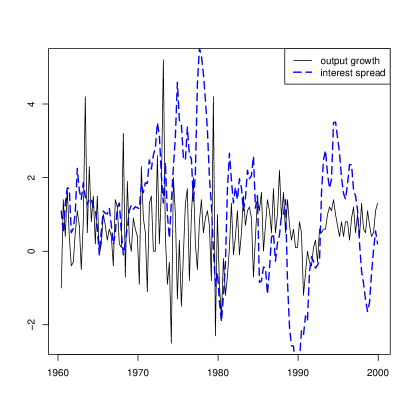
Figure 1: UK output growth and interest spread, quarterly data from 1960:3 to 1999:4

Estimating by ML, we obtain the following coefficients

$$\hat{b}=(0.35,0.21,0.15,0.32,−0.52,2.56,0.68,0.20,−0.14,1.14,−0.26)′,$$

and standard errors

$$s.e.(\hat{b})=(0.09,0.09,0.09,0.11,0.15,0.29,0.12,0.09,0.10,0.10,0.10)$$

(calculated using residual parametric bootstrap with $10000$ draws) and construct corresponding matrices $\hat{B}_{1}$ and $\hat{B}_{2}$. Imposing stationary initial values in the estimation is not feasible because for the considered LSTAR model (as well as most other nonlinear (V)AR models) the stationary distribution is not known. Thus, the ML estimation employed is necessarily conditional on fixed (and known) initial values.

The maximum eigenvalues of $\hat{B}_{1}$ and $\hat{B}_{2}$ are $0.9216$ and $0.8236$, both below $1$, therefore the necessary condition of Assumption R^′ is satisfied. To obtain bounds on the joint spectral radius we use the JSR toolbox written in Matlab by Raphael Jungers, freely downloadable (with documentation and demos) from Matlab Central (https://www.mathworks.com/matlabcentral/fileexchange/33202-the-jsr-toolbox) The toolbox is described in Vankeerberghen, Hendrickx and Jungers (2014). In our case, the toolbox provides the upper and lower bounds which coincide up to the 4th digit and the value is $0.9216$, calculated in 9 iterations in 31 seconds. Therefore, Assumption R^′ is satisfied.

Notice that the last column of both matrices consists of zeros. That means that the set $\{B_{1},B_{2}\}$ is reducible to $\{B_{1,1},B_{2,1}\}$ (the other two matrices are $1$ by $1$ zeros):

$$B_{1,1}=\begin{pmatrix}0&b_{4}-b_{5}&b_{2}&0&b_{3}\\ 0&b_{10}&0&b_{11}&b_{9}\\ 1&0&0&0&0\\ 0&1&0&0&0\\ 0&0&1&0&0\\ \end{pmatrix}$$

$$B_{2,1}=\begin{pmatrix}0&b_{4}&b_{2}&0&b_{3}\\ 0&b_{10}&0&b_{11}&b_{9}\\ 1&0&0&0&0\\ 0&1&0&0&0\\ 0&0&1&0&0\\ \end{pmatrix}$$

so $\rho\{B_{1},B_{2}\}=\rho\{B_{1,1},B_{2,1}\}$ by Lemma 3 and 4. The JSR toolbox performs this reduction.

4 Main Result

We now state our general result for a model with $g+1$ regimes and heteroskedasticic errors,

$$\begin{split}y_{t}=&\mu_{0}+\sum_{j=1}^{p}\Phi_{j}y_{t-j}+\sum_{i=1}^{g}G_{i}(\gamma,c;s_{t})\left\{\mu_{i}+\sum_{j=1}^{p}\Psi_{i,j}y_{t-j}\right\}\\ &+\left\{\left(1-\sum_{i=1}^{g}G_{i}(\gamma,c;s_{t})\right)\Omega_{0}+\sum_{i=1}^{g}G_{i}(\gamma,c;s_{t})\Omega_{i}\right\}^{1/2}\varepsilon_{t},\end{split}$$ (5)

where $y_{t}$ and $\varepsilon_{t}$ are $n\times 1$ random vectors, $\mu_{0}$ and $\mu_{i}$ are $n\times 1$ intercept vectors, $\Phi_{j}$ and $\Psi_{i,j}$, $j=1,\ldots,p$, are $n\times n$ parameter matrices, and $\Omega_{i}$ is positive definite and $i=1,\ldots,g$. We assume that random vectors $\varepsilon_{t}$ are i.i.d.$(0,I_{n})$ with a density bounded away from zero on compact subsets of $R^{n}$. If regime switches are only in conditional means, i.e. variances coincide in all regimes, $\Omega_{0}=\Omega_{i}$ for all $i=1,\ldots,g$, then the last term is simplified to $\Omega_{0}^{1/2}\varepsilon_{t}$. The transition function is common for all components of vector $y_{t}$, and it is a continuous function of random variable $s_{t}$ and parameters $\gamma$ and $c$ and takes values on $[0,1]$. Moreover, $G_{1}+...+G_{g}\leq 1$ and $s_{t}$ is a function of $\{y_{t-j},j=1,\ldots,p\}$ as before.

For $i=1,\ldots,g$ define matrices

$$B_{i}=\begin{pmatrix}\Phi_{1}+\Psi_{i,1}&\Phi_{2}+\Psi_{i,2}&\cdots&\Phi_{p-1}+\Psi_{i,p-1}&\Phi_{p}+\Psi_{p}\\ I_{n}&0&\cdots&0&0\\ 0&I_{n}&\cdots&0&0\\ \vdots&\vdots&\ddots&\vdots&\vdots\\ 0&0&\cdots&I_{n}&0\end{pmatrix}$$

$$B_{g+1}=\begin{pmatrix}\Phi_{1}&\Phi_{2}&\cdots&\Phi_{p-1}&\Phi_{p}\\ I_{n}&0&\cdots&0&0\\ 0&I_{n}&\cdots&0&0\\ \vdots&\vdots&\ddots&\vdots&\vdots\\ 0&0&\cdots&I_{n}&0\end{pmatrix}$$

Assumption R The joint spectral radius of the matrices defined above is less than $1$, i.e. $\rho(\{B_{1},\ldots,B_{g},B_{g+1}\})<1$.

We will use the Markov chain theory on which Mayen and Tweedie (1993) is a standard reference. In particular, for geometric ergodicity of a Markov chain see Meyn and Tweedie (1993), Chapter 15.

Theorem 1.

Suppose that Assumption R is satisfied. Then the process $Z_{t}=\{y^{\prime}_{t},\ldots,y^{\prime}_{t-p+1}\}$ is a $(1+\|x\|^{2})$-geometrically ergodic Markov chain. Therefore, there exist initial values $y^{\prime}_{t-p+1},\ldots,y_{0}^{\prime}$ such that the process $y_{t}$ defined in (5) is 1) strictly stationary 2) second-order stationary 3) $\beta$-mixing with geometrically decaying mixing numbers.

Proof.

Saikkonen (2008) establishes stationarity and mixing properties of nonlinear vector error correction (VEC) models under Assumption R using the theory of Markov chains. In order to do so, he transforms the VEC model into a VAR model which can be formulated as a Markov chain for which Theorem 15.0.1 of Meyn and Tweedie (1993) can be applied. The main work is to verify condition (15.3) and related assumptions of that theorem. As our model is already a VAR model, it is sufficient to show that our vector STAR model can be written in the form of the nonlinear VAR model in Equation (17) of Saikkonen (2008) and that the assumptions needed in Theorem 1 of that paper hold true.

First assume that the number of unit roots $n-r$ in Saikkonen’s Assumption 3 is zero so that $n=r$ (in that assumption $n$ has the same meaning as here). Then note that in the definition of the matrix $J$ above Saikkonen’s Equation (17) we have (in addition to $n=r$) $\beta=c=I_{n}$ and $z_{t}=y_{t}$ (see Saikkonen’s Note 2). Thus, it follows that $J$ is a nonsingular matrix of dimension $np$ and we can choose the matrix $S$ in Equation (17) the inverse of $J^{\prime}$. In Saikkonen’s Equation (17) $h_{1}+...+h_{m}=1$ and we assume that, corresponding to Saikkonen’s Assumption 2, the functions $h_{s}$ are independent of the argument $\eta_{t}$. Then, with $m=g+1$ the first term on the right hand side of Equation (17) in Saikkonen (2008) is

$$\sum_{s=1}^{m}h_{s}\sum_{j=1}^{p}\bar{B}_{sj}y_{t-j}=\sum_{j=1}^{p}\bar{B}_{g+1,j}y_{t-j}+\sum_{i=1}^{g}h_{i}\sum_{j=1}^{p}(\bar{B}_{ij}-\bar{B}_{g+1,j})y_{t-j}.$$ (6)

Substitute $h_{m}=1-\sum_{i=1}^{g}G_{i}$, $h_{i}=G_{i}$ and $\bar{B}_{g+1,j}=\Phi_{j}$ and $\bar{B}_{ij}-\bar{B}_{g+1,j}=\Psi_{i,j}$ to obtain dynamics in Equation (5) without the intercept. The second term, which is defined in Equation (11) in Saikkonen (2008), produces the intercept, because we can take $\rm{I}_{2}$ as an empty set of indexes. Finally, the third term gives the required heteroskedastic errors, because

$$\sum_{s=1}^{m}h_{s}\Omega_{s}=\left(1-\sum_{=1}^{g}G_{i}\right)\Omega_{0}+\sum_{i=1}^{g}G_{i}\Omega_{i}.$$ (7)

From the preceding discussion and the fact that the random variable $s_{t}$ is a function of $\{y_{t-j},j=1,\ldots,p\}$ we can conclude that Equation (5) is a special case of Equation (17) of Saikkonen (2008). Therefore Markov chain theory for the process $Z_{t}=\{y^{\prime}_{t},\ldots,y^{\prime}_{t-p+1}\}$ can be applied. The conditions assumed for the error term and transition functions below Equation (5) imply that the conditions in Assumptions 1 and 2(a) of Saikkonen (2008) are satisfied whereas condition (b) in his Assumption 2 is dispensable. To see that Theorem 1 of Saikkonen (2008) implies the assertions stated in our theorem it now suffices to note that our Assumption R corresponds to Saikkonen’s (2008) condition (19) and his Equation (10) is dispensable in our case. ∎

5 Final Remarks

In this paper we describe conditions for stationarity and ergodicity of vector STAR models. The sufficient condition is that the joint spectral radius of certain matrices is below $1$. This condition can be checked using recently introduced toolboxes from computational mathematics.

For linear models, for example for the (causal) univariate autoregressive model of order $1$, it is known that stationarity holds if the autoregressive coefficient is in $(-1,1)$, otherwise the time series is nonstationary. For the considered vector LSTAR model, the stationarity holds if the joint spectral radius is below $1$. However, it is only a sufficient condition for stationarity and ergodicity. Thus, if the joint spectral radius equals one or is larger than one, we can only conclude that it is not possible to verify stationarity and ergodicity by using the employed criterion and in principle it is possible that stationarity and ergodicity still holds. The conclusion is similar to that discussed above if the value of the joint spectral radius based on estimates is smaller than one but deemed to be so close to one that, due to estimation errors, it can be one or even larger than one with high probability.

An interesting extension of the model considered here would be to add regressors $x_{t}$, as in e.g. Hubrich and Terasvirta (2013)

$$y_{t}=\mu_{0}+\sum_{j=1}^{p}\Phi_{j}y_{t-j}+\Gamma x_{t}+G(\gamma,c;s_{t})\left\{\mu_{1}+\sum_{j=1}^{p}\Psi_{j}y_{t-j}+\Xi x_{t}\right\}+\varepsilon_{t},$$ (8)

where $x_{t}$ are $k\times 1$ random vectors, $\Gamma$ and $\Xi$ are $n\times k$ parameter matrices. Suppose that $x_{t}$ is an exogenous random vector. Then no results on stationarity can hold true if $x_{t}$ is nonstationary, and even if $x_{t}$ is assumed stationary and ergodic Theorem 1 in Saikkonen (2008) is not applicable because without further assumptions model (8) cannot be cast into the required Markov chain form.

6 Acknowledgements

Igor Kheifets gratefully acknowledges financial support from the Spanish Ministerio de Ciencia, Innovacion y Universidades under Grant ECO2017-86009-P and thanks the faculty and staff of the New Economic School for their hospitality during his visits to Moscow. Pentti Saikkonen thanks the Academy of Finland (grant number 1308628) for financial support.

References

- [1] Anderson, H. M., Athanasopoulos, G. and Vahid, F. (2007), Nonlinear autoregressive leading indicator models of output in G-7 countries. Journal of Applied Econometrics 22, 63–87.
- [2] Bec, F. and A. Rahbek (2004) Vector equilibrium correction models with non-linear discontinuous adjustments. Econometrics Journal 7, 628–651.
- [3] Blondel, V.D. and Y. Nesterov (2005) Computationally efficient approximations of the joint spectral radius. SIAM Journal of Matrix Analysis 27, 256–272.
- [4] Gripenberg, G. (1997) Computing the joint spectral radius. Linear Algebra and Its Applications 234, 43–60.
- [5] Hubrich, K. and T. Terasvirta (2013) Thresholds and Smooth Transitions in Vector Autoregressive Models. VAR Models in Macroeconomics – New Developments and Applications: Essays in Honor of Christopher A. Sims. 273–326.
- [6] Jungers R. M. (2009) The joint spectral radius, Theory and applications. In Lecture Notes in Control and Information Sciences, volume 385. Springer-Verlag, Berlin.
- [7] Kheifets, I (2018) Multivariate Specification Tests Based on the Dynamic Rosenblatt Transform. Computational Statistics & Data Analysis 124, 1–14.
- [8] Liebscher E. (2005) Towards a Unified Approach for Proving Geometric Ergodicity and Mixing Properties of Nonlinear Autoregressive Processes. Journal of Time Series Analysis 26, 669–689.
- [9] Meyn, S.P. and R.L. Tweedie (1993) Markov Chains and Stochastic Stability. Springer-Verlag, Berlin.
- [10] Protasov V.Y. (1996) The joint spectral radius and invariant sets of linear operators. Fundamentalnaya i prikladnaya matematika, 2, 205–231.
- [11] Saikkonen, P. (2005) Stability results for nonlinear error correction models. Journal of Econometrics 127, 69–81.
- [12] Saikkonen, P. (2008). Stability of regime switching error correction models under linear cointegration. Econometric Theory 24, 294–318.
- [13] Vankeerberghen, G. and Hendrickx, J. and Jungers, R. M. (2014) JSR: A Toolbox to Compute the Joint Spectral Radius. In Proceedings of the 17th International Conference on Hybrid Systems: Computation and Control. 151–156.