In the IP of the Beholder: Strategies for Active IPv6 Topology Discovery

In the IP of the Beholder: Strategies for Active IPv6 Topology Discovery

Abstract.

Existing methods for active topology discovery within the IPv6 Internet largely mirror those of IPv4. In light of the large and sparsely populated address space, in conjunction with aggressive ICMPv6 rate limiting by routers, this work develops a different approach to Internet-wide IPv6 topology mapping. We adopt randomized probing techniques in order to distribute probing load, minimize the effects of rate limiting, and probe at higher rates. Second, we extensively analyze the efficiency and efficacy of various IPv6 hitlists and target generation methods when used for topology discovery, and synthesize new target lists based on our empirical results to provide both breadth (coverage across networks) and depth (to find potential subnetting). Employing our probing strategy, we discover more than 1.3M IPv6 router interface addresses from a single vantage point. Finally, we share our prober implementation, synthesized target lists, and discovered IPv6 topology results.

1. Introduction

As of August 2018, about 23% of Google’s users access their services via IPv6 (Google, 2018), while APNIC reports that $\sim$16k Autonomous Systems (ASes) advertise IPv6 prefixes (Huston, 2018). The number of IPv6 routes in the BGP system has increased from $\sim$5k in 2011 to more than 56k today (Huston, 2018), while native IPv6 adoption and traffic continues its exponential increase (Czyz et al., 2014). Similarly, a large content delivery network (CDN) observed 1.72B unique native IPv6 addresses for 576 million unique /64 prefixes on March 17, 2018 (Plonka and Rose, 2017). In a weeks’ time, the number of IPv6 /64s covering active WWW clients approximated the total number of globally routed IPv4 unicast addresses ($\sim$2.5B). These examples underscore the importance of IPv6 today, and the need for accurate IPv6 topologies within the community.

Understanding the Internet’s IPv6 topology is important for applications ranging from improved content distribution and traffic optimization, to better address anonymization (Plonka and Berger, 2017) and reputation (Collins et al., 2007; Kalafut et al., 2010), to enhanced network security (Zhang et al., 2008; Syamkumar et al., 2016). Despite these compelling applications, three challenges remain: (i) an infeasibly large address space that cannot be exhaustively scanned or uniformly sampled effectively, (ii) mandated and aggressive ICMPv6 rate limiting in routers (Conta et al., 2006), and (iii) unknown address allocation policies and subnet structures. Note that the first two issues are inter-related: attempting to increase coverage by probing more of the IPv6 address space necessitates faster probing rates. However, increasing the probing rate is self-defeating as doing so triggers more rate limiting and, hence, fewer discovered router interfaces and less representative topologies.

While decades of research have developed and refined active IPv4 topology discovery (e.g.,  (Spring et al., 2002; k. claffy et al., 2009; Donnet et al., 2005; Keys, 2010; Beverly et al., 2010), these techniques do not address the aforementioned challenges unique to IPv6. Existing IPv6 topology mapping systems are thus forced to directly apply IPv4 discovery tools and techniques. For example, production CAIDA and RIPE traceroutes regularly probe the ::1 address of every global IPv6 BGP prefix (CAIDA, 2018b; RIPE NCC, 2018). Because of this very sparse sampling within the large IPv6 address space, the completeness and quality of the resulting logical topologies is unknown.

In this work, we seek to advance the state-of-the-art in Internet-wide IPv6 active topology mapping. Our methodology tackles two fundamental aspects of the problem: (i) which addresses to target; and (ii) how to probe.

First, we amass the largest collection of IPv6 target addresses/seeds currently available from a variety of sources (e.g., BGP, DNS, CDNs (Fiebig et al., 2017; Rapid7, 2018; Security, 2018; Gasser et al., 2016; Plonka and Berger, 2017)) as well as generated seeds (e.g., 6Gen (Murdock et al., 2017)). We employ a three-step process to synthesize 12.4M target addresses specifically crafted to promote topology discovery. Next, we perform a total of 45.8M traces from three vantages: two US universities and one EU network. We investigate different target selection methods and parameters (e.g., maximum TTL, protocol, probing speed, etc.) to find those that elicit the most IPv6 topological information. We show that our methodology provides breadth across networks, depth to discover subnetting, and speed. Employing our probing strategy, we discover $>$1.3M IPv6 router interface addresses from a single vantage point in a single day – an order of magnitude more than produced by current state-of-the-art mapping systems that use hundreds of vantages in the same period. Our primary contributions thus include:

• Evaluation of various means to synthesize target addresses from seven different input seed sets.

• Quantification of random probing to maintain high rates while avoiding ICMPv6 rate limiting.

• Characterization of target list power to yield topological results.

• IPv6 subnet discovery as a case study of topological inference.

• IPv6 router interface-level topology results, our synthesized target lists, and our prober implementation (Beverly and Rohrer, 2018).

The remainder of this paper is organized as follows. Section 2 provides background on IPv6 topology mapping, while Section 3 characterizes the seed lists we utilize and describes our method for synthesizing an IPv6 target set. We describe our probing in Section 4, and provide results from an Internet-wide probing campaign in Section 5. Section 6 analyzes the results to infer likely subnetting and better understand provider provisioning. We conclude in Section 7 with a discussion of the security and privacy implications of our work, as well as suggestions for continued research.

2. Background and Related Work

IPv4 topology. Since the seminal Mercator (Govindan and Tangmunarunkit, 2000) and Rocketfuel work (Spring et al., 2002), the measurement community has made continual progress toward improving IPv4 topology discovery and inference (see e.g., (k. claffy et al., 2009; Keys, 2010; Beverly et al., 2010) and references therein). Related to our initiative to design a scalable active topology mapping system, Doubletree (Donnet et al., 2005) begins tracing from a midpoint on the path and halts when a trace reaches a known, previously probed portion of the path. We examine Doubletree’s performance for IPv6 in Section 4.2.

Recently, Beverly introduced Yarrp, a randomized high-speed IPv4 topology prober (Beverly, 2016). In contrast to traditional traceroute techniques intended to probe individual paths, Yarrp spreads topology probes across the network rather than probing the path to each individual destination sequentially. It does this by randomly permuting the space of destination targets and TTLs, thereby attempting to avoid overloading any single router or path. In addition, Yarrp is stateless and can recover the necessary information to match replies via carefully crafted probes. These properties allow Yarrp to perform high-speed topology mapping. For instance, Yarrp has been run at $100kpps$ to discover more than $400k$ unique IPv4 router addresses in approximately 23 minutes (Beverly, 2016).

Despite the significant body of prior work on IPv4 topology, IPv6 has at least two fundamental differences: a much larger address space (that is sparsely populated) and aggressive ICMPv6 rate limiting (Conta et al., 2006; Kahn et al., 2018). We explore new techniques to accommodate both of these properties in this work.

IPv6 topology. Dhamdhere et al. studied the evolution of IPv6 topology at the AS-level using passive BGP data and found that fewer than 50% of AS-level paths in 2012 were identical between IPv4 and IPv6, while a single AS (Hurricane Electric) appeared in 20-95% of observed IPv6 AS paths (Dhamdhere et al., 2012). Similarly, Czyz et al. examined BGP tables in 2013 and, while they found only 19% of ASes supporting IPv6, a k-core analysis showed that these ASes were well-connected large networks with high centrality (Czyz et al., 2014). Complementary to these efforts, we take an in-depth look at the IPv6 topology, starting from an interface-level perspective, after a period of sustained growth, via active probing.

Presently, two production measurement platforms continually perform active IPv6 topology mapping: CAIDA’s Ark (CAIDA, 2018b) and RIPE Atlas (RIPE NCC, 2018). These systems send Paris (Augustin et al., 2006) traceroute probes toward the ::1 address in each IPv6 prefix present in the global BGP table. Ark also probes a random address in each prefix. A central finding of our work is that using BGP prefixes alone to guide target selection works well to capture topological breadth, but not depth, i.e., it does not discover subnetting.

Rohrer et al. uniformly sampled the IPv6 Internet in 2015 by tracerouting to an address in every /48 prefix that makes up the routed IPv6 address space (Rohrer et al., 2016). Their study issued ten times as many traces as our work, yet found an order of magnitude fewer interfaces – demonstrating the necessity to perform finer-grained probing within some prefixes to discover extant subnetting and the routers supporting the subnets.

More broadly, prior studies of IPv6 topology use traditional tools including traceroute6 (Malone, 2008) and scamper (Luckie, 2010). Gaston was the first to explore higher-rate IPv6 active topology probing (Gaston, 2017) via randomization, and demonstrated the ability to capture roughly an equivalent amount of topological information as collected via CAIDA’s Ark system. However, Gaston’s study did not examine the critical problem of target selection and rate-limiting, and did not explore the ability to utilize high-speed probing to discover a larger swath of the topology. Alvarez et al. developed and evaluated methods to deal with ICMPv6 rate-limiting problems, but in a stateful, proprietary prober (Alvarez et al., 2017).

Separate to interface-level topology discovery is finding aliases, i.e., determining those interfaces that belong to the same physical router, and creating router-level graphs. Luckie et al. developed speedtrap, the first Internet-scale IPv6 alias resolution technique (Luckie et al., 2013), now used to produce router-level graphs of the IPv6 Internet as part of CAIDA’s ITDK (CAIDA, 2018a). In this work, we focus on IPv6 interface address discovery, and do not perform alias resolution. However, as alias resolution takes interface addresses as input, the ability to discover IPv6 interfaces is directly beneficial (Padmanabhan et al., 2015).

IPv6 hitlists. Catalogs of active IPv6 addresses in the Internet, commonly known as hitlists, have been of interest to the measurement community over the last decade. Notable efforts leverage active (e.g., random probing of ::1 (CAIDA, 2018b), exhaustive probing of ::1 address in each /48 in all advertised /32s (Rohrer et al., 2016), and reverse DNS zone walking (Fiebig et al., 2017; Borgolte et al., 2018)) and passive techniques (e.g., from BGP updates (Dhamdhere et al., 2012; Huston, 2018) and from traffic captures (Dainotti et al., 2013)) as well as a number of passive and active sources (Gasser et al., 2016). Similar to our effort, Gasser et al. observe the propensity of IPv6 hitlists to contain clusters of addresses (Gasser et al., 2018). While Gasser provides a new, aggregate IPv6 hitlist that also removes aliased prefixes, they do not study how to adapt the hitlist to IPv6 topology discovery. We provide details of the specific hitlists we utilize in Section 3.1.

IPv6 addresses and deployments. Many issues pertinent to our work – including address seed sources, target selection, and probing techniques – reflect current understanding of IPv6 network reconnaissance (Gont and Chown, 2016). Malone analyzes different aspects of three IPv6 address datasets and presents an analysis technique to learn about their deployments and usages (Malone, 2008). Czyz et al. (Czyz et al., 2016) studied 520k and 25k dual-stacked servers and routers respectively and compared the security policies of IPv4 and IPv6 deployments. To assess the lifetime and density of IPv6 addresses, Plonka and Berger developed Multi-Resolution Aggregate plots and classified billions of addresses spatially and temporally (Plonka and Berger, 2015). A recursive algorithm to discover and extract IPv6 addressing patterns is discussed in (Ullrich et al., 2015). Similarly, Foremski et al. proposed the Entropy/IP system to uncover the structure of IPv6 addresses using machine learning (Foremski et al., 2016). In a like vein, Murdock et al. designed “6Gen” target generation  (Murdock et al., 2017). 6Gen exploits address locality: discovery of new targets happens closer to highly dense ranges. In a nybble, targets are generated either based on a specific range (e.g., 2::[1-4]:0) or wildcard (e.g., 2::?:0); the former is tight clustering while the latter is referred as loose.

Figure 1. IPv6 topology target generation: addresses from various seeds are transformed into intermediate prefixes which are then synthesized into targets.

3. Target Selection

Our methodology tackles two primary challenges: (i) selecting targets from the large and sparsely populated IPv6 address space; and (ii) effectively probing. This section considers target selection.

Table 1. Seed List Properties

Name	Method	Date	# Addrs	Interface Identifiers (IIDs)
		yyyy/mm/dd		Random		LowByte		EUI-64
CAIDA (CAIDA, 2018b)	BGP-derived	2018/05/09	105.2k	53.7k	$51.02\%$	51.5k	$48.98\%$	0	$0.00\%$
DNSDB (Security, 2018)	Passive DNS	2018/02/15 – 2018/04/28	5.4M	1.3M	$24.43\%$	2.2M	$41.27\%$	146.5k	$2.74\%$
Fiebig (Fiebig et al., 2017)	Reverse DNS	2018/03/27	11.7M	4.2M	$35.94\%$	3.2M	$27.54\%$	275.4k	$2.35\%$
FDNS (Rapid7, 2018)	Fwd. DNS	2018/04/27	24.8M	3.3M	$13.12\%$	7.0M	$28.20\%$	236.8k	$0.95\%$
CDN Clients(Plonka and Berger, 2017)	kIP anonymization: $k=256$	2018/02/18 – 2018/03/03	N/A	All	$100.00\%$	0	$0.00\%$	0	$0.00\%$
	kIP anonymization: $k=32$	2018/02/18 – 2018/03/03	N/A	All	$100.00\%$	0	$0.00\%$	0	$0.00\%$
6gen (Murdock et al., 2017)	Generative	2018/03/13	4.9M	4.4M	$89.61\%$	389.2k	$7.93\%$	17.1k	$0.35\%$
Combined	Join Sets	varies	50.8M	13.2M	$28.19\%$	12.9M	$27.45\%$	675.8k	$1.44\%$
TUM (Gasser et al., 2016)	Collection	varies	5.6M	2.3M	$44.62\%$	1.2M	$23.54\%$	604.0k	$11.79\%$
Random	Random	2018/05/23	26.5M	0	$0.0\%$	95.8k	$0.36\%$	0	$0.0\%$

3.1. Target Generation

We employ a three step process, outlined in Figure 1, to prepare a set of targets, based on a set of intermediate prefixes, which are synthesized from seeds. The targets are IP addresses to be used as destinations for TTL-limited probes emitted from a vantage. When discussing IPv6 addresses, we adopt the standard vernacular of a subnet prefix to denote the high-order bits and the interface identifier (IID) to denote the least significant 64 bits (Hinden and Deering, 2006).

Step 1: Seed Sourcing. A list of seeds is obtained from a source. Our seeds are either IP prefixes (base address and length) or IPv6 addresses (base address with implicit 128bit length), which are used as hints to select interesting areas of the address space that help define probe destinations.

Step 2: Prefix Transformation. One or more transformations may be applied to the seeds to yield a set of intermediate prefixes. Depending on the transformation method, the resulting set might have the same or fewer number of prefixes than the seed list to which it was applied. The prefix transformations we use are:

• kn: Perform kIP aggregation-based address anomymization with parameters: $w=14$ (window days), $i=1$ (interval hours), $k=n$ (simultaneously-assigned /64 prefixes), $p=50$ (50th percentile of intervals). (Plonka and Berger, 2017), e.g., k32 and k256 (Plonka and Berger, 2017).

• zn: Extend input prefixes with length $<n$ to /n, i.e., base address set to zeroes after the nth bit; aggregate input prefixes having length $>n$ to /n prefixes.

Step 3: Target Synthesis. Lastly, a synthesis method takes the intermediate prefixes as input and yields a set of target addresses. The target synthesis methods used in this study are as follows:

• lowbyte1: bitwise OR prefix base address with IID value
  :0000:0000:0000:0001.

• fixediid: bitwise OR prefix base address with IID value
  :1234:5678:1234:5678.

For each, we remove duplicate addresses within the set. The target address sets are then ready to be employed in a probe campaign.

3.2. Seeds

The seed sources used in this study are as follows:

• caida: The set of probe targets selected by CAIDA, based on BGP-advertised IPv6 prefixes of size /48 or larger, i.e., prefixes with length of at most 48 bits (CAIDA, 2018b).

• fiebig: The set of IPv6 addresses gleaned from walking the ip6.arpa zones in the DNS (Fiebig et al., 2017).

• fdns_any: A set of IPv6 addresses found in DNS answers in response to forward DNS ANY queries performed by Rapid7’s Project Sonar (Rapid7, 2018).

• dnsdb: A set of IPv6 addresses found in DNS answers passively observed in AAAA DNS query responses by Farsight Security’s Farsight Passive DNS project, anonymized and imported into Farsight DNSDB (Security, 2018). We queried DNSDB for all IPv6 records observed between 15 Feb and 28 Apr 2018 in the covering set of all advertised BGP IPv6 prefixes (as reported by RouteViews (rou, 2016) on 20 Apr 2018).

• cdn: A set of IPv6 prefixes, having various lengths, that are anonymized aggregates (Plonka and Berger, 2017) covering WWW client IPv6 addresses believed to be SLAAC temporary privacy addresses (the most common type of WWW client addresses (Plonka and Berger, 2015)), as observed by a large Content Delivery Network (CDN) across 14 days, February 18, 2018 through March 3, 2018 (UTC).

• 6gen: A set of IPv6 address synthesized using the 6Gen tool in loose clustering mode (Murdock et al., 2017). The input to the tool is a combination of IPv6 destinations probed and new interfaces found from probing those destinations by CAIDA on March 06, 2018.

• tum: A combined set of IPv6 addresses created by combining multiple existing address sets including some that we also use individually (fdns_any) and a number of others (openipmap, ct, caida-dnsnames, alexa-country, traceroute, and traceoute-v6-builtin). Some of these subsets are documented in (Gasser et al., 2016) and others are undocumented. Each subset is packaged separately, and we noted some anomalies (such as zero-size of very small files for recent dates) leaving room for interpretation as to what would best represent the TUM dataset as a whole. With this in mind we took the most recent and largest file for each subset, which are shown in Table 2.

  Table 2. TUM Seed Subsets

  Filename	# Addresses
  alexa-country-2018-04-23.csv	1,634
  caida-dnsnames-2018-01-17.csv	1,268,982
  caida-dnsnames-2018-04-25.csv	16,507
  ct-2018-04-27.csv	21,983,387
  openipmap-2018-04-23.txt	11,149
  rapid7-dnsany-2018-03-30.csv	24,959,477
  rapid7-dnsany-2018-03-31.csv	14,434,117
  traceroute-2018-04-24.txt	128,398
  traceroute-v6-builtin-2018-02-25.txt	112,754
  All zone files from 2018-04-27	17,173,243
  Total	80,089,648
  Total Unique	5,599,313

We examine several features of our seed lists in Table 1. At a glance we note the wide variance in size (105k addresses to 25M). The seeds are derived using widely varying methodologies, which we hope makes them complementary (not redundant). We also perform a simple classification of the IIDs in order to inform our choice of target IID, as well as enable correlation with result sets.

We classified our seed addresses using the addr6 tool (SI6 Networks, 2016). This tool examines each address, looking for patterns, such as whether the IID, e.g., (i) may be an EUI-64 IID with an embedded MAC address, (ii) has a run of zeroes followed only by a low number (“lowbyte”), or (iii) has no discernible pattern (“randomized”, essentially meaning unrecognized). In Table 1, the percentages reflect the proportion within each seed list (row).

The CDN clients’ individual IPv6 addresses were not provided to the authors in order to maintain privacy; instead, the authors received and utilized anonymized prefixes that were generated using the kIP aggregation approach as mentioned in Section 3.1. While the number of addresses aggregated is undisclosed, there were 421,807 aggregates (prefixes) in the CDN-k256 set and 3,445,329 in the CDN-k32 set. We treat the first six seed lists in Table 1 as independent. We create our own combined list by joining those six lists. The TUM list is also a collection (Gasser et al., 2016), which includes CAIDA and FDNS subsets, and therefore is not independent of the first six lists. Lastly, we randomly generate 26.5M targets in BGP routed IPv6 address space as a control seed list.

3.3. Selecting Transformations

Prefix transformation granularity. Next, we seek to understand the influence of aggregation granularity when performing prefix transformation. Many of our seed input datasets contain multiple IPv6 addresses within the same /64 prefix – this is a natural consequence of their intended use as hitlists for IPv6 host discovery, rather than IPv6 router discovery. Intuitively, assuming that /64 prefixes are allocated to LANs or Internet service subscribers as the smallest common IPv6 subnets, we would not typically expect traceroutes to multiple addresses within the same /64 to yield different topologies.

To characterize the relationship to the discovered topology, and the probing required when using our zn transformation, we mounted a trial campaign that probed the fdns_any dataset for varying values of $n$. Table 3 shows that z64 requires more than eight times as many probes as z40, but discovers three times as many unique interfaces. More importantly, we consider the number of interfaces that are discovered exclusively as a result of using a particular transformation level. Although z64 requires significant probing, there are more than 27k interfaces that were only discovered when using this transformation level. Finally, we examine the number of non-“Time Exceeded” responses from each of the levels. The fraction of other ICMPv6 responses per probe is 0.012, 0.029, 0.032, and 0.041 for $n=40,48,56,64$, respectively. Thus, after normalizing to the number of probes, the $n=64$ transformation level has the effect of producing a higher rate of non-“Time exceeded” responses, suggesting that these probes are reaching deeper into networks.

Table 3. ICMPv6 Trial Results by Transformation

zn	Probes	Other ICMPv6	Addrs	Excl Addrs
/40	1.4M	17.5k	27.0k	158
/48	3.6M	105.8k	45.5k	321
/56	6.1M	194.8k	60.5k	1.1k
/64	11.8M	486.8k	85.5k	27.2k

Target synthesis. The lower 64 bits of an IPv6 address denote the interface identifier (IID) (Hinden and Deering, 2006). Given a candidate prefix, we must select an IID within that prefix to probe. Natural candidates are the IID ::1, a random IID, an IID occurring in the input seed list, or a (optionally fixed) pseudo-random identifier. In addition to understanding whether this choice has an impact on topological discovery, we further wish to expose the extent to which different identifiers elicit non-“Time Exceeded” messages as a metric of impact on hosts. We therefore mounted two trial campaigns using the cdn-k256 prefixes, the z64 transformation, and both the (a) lowbyte1 and (b) fixediid host identifiers for target synthesis. Table 4 shows the distribution of ICMPv6 Time Exceeded and Destination Unreachable responses received as a result of the campaigns.

Table 4. ICMPv6 Trial Results by IID

type/code	CDN-k256 z64		Fiebig
	lowbyte1	fixediid	known
Time Exceeded	98.1%	98.1%	95.8%
no route to destination	0.7%	0.7%	0.6%
administratively prohibited	0.6%	0.6%	0.4%
address unreachable	0.3%	0.4%	0.7%
port unreachable	0.1%	0.0%	2.3%
reject route to destination	0.1%	0.2%	0.2%

First, we find that more than 98% of responses are ICMPv6 time exceeded messages as we expect. We see only negligible differences between lowbyte1 and fixediid; lowbyte1 produces five times as many ICMPv6 port unreachable responses, but the total number of such responses is still very small. Second, to understand the use of a known address within the prefix, we further compare against probes toward known addresses within the Fiebig seed list (not shown). In contrast to probing the ::1 or fixed, these port unreachable messages constitute 2.3% of the distribution for the known address probing, suggesting that our probing is reaching end hosts.

Because we observe only minimal impact on discovery between fixed IID and the ::1 IID (a response rate difference of less than 2%), we choose to use the fixed identifier for the remainder of the experiments in order to minimize any potential impacts from probes reaching end hosts.

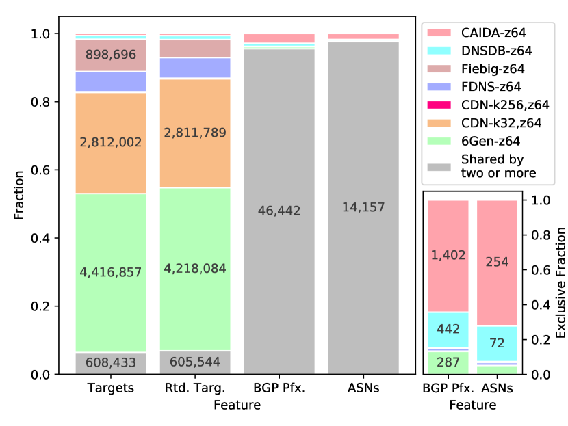
Figure 2. Features contributed by each target set

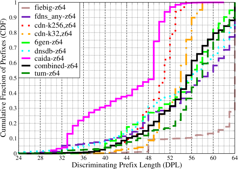
(a) DPL distribution for addresses in each set

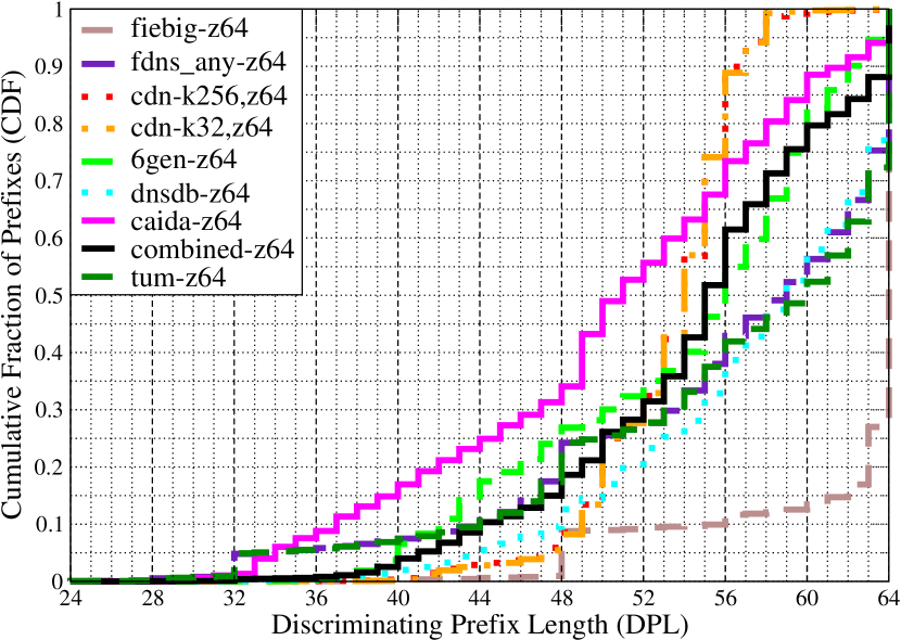
(b) DPL distribution when sets are considered together

Figure 3. Discriminating Prefix Length (DPL) Distributions for target sets (CDF)

Table 5. Target Set Properties

Name	Agg	Unique	Exclusive	Routed	Exclusive	BGP	Exclusive	ASNs	Exclusive	6to4
		Targets	Targets	Targets	Routed Targs	Prefixes	BGP		ASNs
CAIDA	z48	78.3k	26.4k	76.2k	25.4k	47.5k	1.4k	14.4k	254	0
	z64	105.2k	56.6k	102.7k	55.2k	47.6k	1.4k	14.4k	254	0
DNSDB	z48	93.8k	9.3k	93.3k	9.4k	36.5k	360	12.8k	73	80
	z64	233.0k	101.1k	231.9k	101.0k	36.7k	442	12.8k	72	80
Fiebig	z48	102.2k	85.4k	45.1k	28.8k	6.0k	8	3.9k	2	0
	z64	1.0M	898.7k	576.9k	468.8k	6.0k	11	3.9k	2	0
FDNS	z48	228.7k	171.8k	193.0k	136.7k	13.4k	17	7.7k	5	88.4k
	z64	746.9k	566.3k	709.9k	530.4k	13.5k	34	7.7k	6	88.5k
CDN-k256	z48	162.4k	2.6k	162.3k	2.6k	3.3k	0	589	0	160
	z64	396.7k	19.6k	396.6k	19.5k	3.3k	0	589	0	160
CDN-k32	z48	524.2k	341.8k	523.9k	341.6k	4.9k	3	1.2k	0	1.4k
	z64	3.2M	2.8M	3.2M	2.8M	4.9k	4	1.2k	0	1.4k
6Gen	z48	1.4M	1.4M	1.3M	1.3M	44.3k	171	13.8k	17	0
	z64	4.5M	4.4M	4.3M	4.2M	44.5k	287	13.8k	18	0
Combined	z48	2.3M	N/A	2.1M	N/A	48.3k	N/A	14.5k	N/A	89.9k
	z64	9.5M	N/A	8.8M	N/A	48.6k	N/A	14.5k	N/A	90.0k
TUM	z48	362.7k	108.4k	305.3k	86.0k	25.6k	36	10.9k	10	91.0k
	z64	2.1M	1.3M	2.0M	1.3M	25.9k	158	10.9k	20	91.2k
Total	z48	2.4M	N/A	2.2M	N/A	48.3k	N/A	14.5k	N/A	100.7k
	z64	10.8M	N/A	10.1M	N/A	48.8k	N/A	14.5k	N/A	100.9k
	both	12.4M	N/A	11.5M	N/A	48.8k	N/A	14.5k	N/A	114.9k

3.4. Target Set Characterization

After generating our target sets as in Section 3.1 and Figure 1, we characterize and compare them across multiple dimensions in Table 5. Unique targets refers to the number of targets in the set after duplicates have been removed. Exclusive (Excl) features are those found only in one of the sets and not any other set. We find that most of the sets have some fraction of targets that are not found in the public BGP IPv6 routing tables, and in some cases (e.g., Fiebig) this fraction is significant, so the “Routed Targets” and “Exclusive Routed Targs” columns characterize only the subset of targets that appear in BGP. Additionally we note that some target sets, despite a large number of targets, are concentrated in only a few BGP prefixes and ASNs, based on the number of BGP prefixes and ASN represented in each set.

As mentioned in Section 3.1, some seed lists, and consequently the corresponding target sets, are not independent of others. When computing features that are exclusive to any of the first 14 sets listed in Table 5 (CAIDA through 6Gen), we do not consider the Combined or TUM sets, since they would mask the exclusive contributions of their respective subsets. For the TUM sets, however, we do show the features that are found in that set exclusively. The Combined and Total sets appear here merely to show the total number of unique features that exist across all sets; they are not independently probed as their own campaigns.

Figure 2 shows the features contributed exclusively by each z64 target set. Clearly there are a few large players in terms of number of targets/routed targets, however this does not strongly correlate to representation in BGP prefixes (Pfx) or ASNs. Since the vast majority of prefixes and ASNs are represented in more than one target set, we provide an alternate inset view of those two features with the shared contribution removed. From this we can see the lack of correlation between target set size and those BGP features.

3.4.1. Discriminating Power

In this work we rely heavily on the notion of address’ discriminating prefix length (DPL). An address’ DPL is the first (leftmost) bit at which it differs from its nearest address accompanying it in a (sorted) set, e.g., one of our target sets. From left to right (high to low order) bits across the address, the DPL is how far one must compare addresses, bit by bit, to discriminate them from each other, for instance how a primitive router might determine which way to forward traffic if two addresses required different treatment. As such, the DPLs of addresses in a set capture their proximity to each other – the higher the DPLs the closer the addresses are – and, when two addresses are topologically heterogeneous, e.g., in different subnets, the addresses’ DPL is a lower bound on their respective subnets’ prefix length. We will first employ DPL to characterize our target sets. Later, in Section 6, we use DPL when discovering network topology from trace results.

Figure 3(a) explores the potential power of each target set to discriminate addresses and subnets, on its own. Note how the distribution of discriminating prefix lengths characterizes a target set. For instance, about 50% of the caida-z64 target addresses have a DPL less than 48, i.e., they do not share the same top 48 bits, and therefore are not covered by the same /48 prefix. In contrast, over 70% of the fiebig-z64 target addresses have DPL of 64, meaning the addresses share the top 63 bits, i.e., are very near one another.

Figure 3(b) explores the increased potential discriminating power that each target set brings when they are used in combination. For example, the caida-z64 distribution shifts right, meaning that some addresses from other target sets are interleaved amongst its target addresses, thus yielding more power to discover router hops on paths to more (specific) routed prefixes or subnets. One might say addresses in some target sets cleave apart addresses in others, yielding a more powerful combined target set in depth as well as breadth. In contrast, note that the distribution of fiebig-z64 is unaffected by the combination. This is largely because it has densely-arranged target addresses, 89% of which are unique (see Table 5) and are not interleaved with those of other target sets.

Note Figure 3(b) allows us to make predictions about the discriminating power of the target sets in combination with each other as measured by a shift rightward to higher DPL values. For instance, cdn-k256,z64 when combined with cdn-k32,z64 discriminating power shifts to that of latter, which happens to contain 94% of the targets in the former. Also, combining fdns_any-z64 with tum-z64 converge to similar discriminating power. Presumably this is a side-effect of the latter largely including the former. Indeed, 88% of the targets in fdns_any-z64 are contained in tum-z64. Additionally, dnsdb-z64 roughly converges with tum-z64 and fdns_any-z64. Given the latter is also DNS-based, it is plausible that it explores some some common address space.

Also noteworthy is what does not change between Figures 3(a) and 3(b). None of the “large” target sets (cdn-k32,z64; 6gen-z64; or tum-z64) shift noticeably to the right. From this we draw two insights. First, combining significantly smaller sets with large sets has no significant impact on the potential discriminating power of the large set (unsurprisingly), even when significant interleaving occurs. Second, none of our large sets interleave significantly with each other. This is both good and bad, meaning that they are complementary in terms of the regions of IPv6 space explored, with the tradeoff being that they do not reinforce one another to enable addition depth of topology discrimination. If two similarly sized and interleaved target sets were combined, we would expect the combined potential discriminating power to be higher than either set individually.

To reiterate, at this stage we are only discussing potential discriminating power because these are only target sets; they are not empirically discovered. While some target sets capture prefixes of real hosts, others are synthetically generated.

4. Probing

We start with Yelling at Random Routers Progressively (Yarrp), a randomized high-speed IPv4 topology prober (Beverly, 2016). Rather than maintaining large amounts of state, as randomization imposes on a traditional traceroute-based prober, Yarrp encodes details of the probe (e.g., originating TTL and timestamp) within the packet so that state can be reconstructed from the ICMP reply. This encoding thus allows Yarrp to be stateless. Yarrp thus decouples probing from topology construction; the complete set of responses to any single destination are not in any order and are intermixed with the responses from all other destinations. Based on promising results measuring IPv4 (Beverly, 2016), we explore adapting these techniques to the IPv6 domain which has both a much larger and sparsely populated address space, as well as mandated ICMPv6 rate limiting.

4.1. Yarrp6

State encoding. IPv6 requires several changes in order to retain the stateless nature of Yarrp. First, IPv6 headers have removed some of the fields used by Yarrp in IPv4 to encode state, e.g., IPID. While there is less room for encoding within the IPv6 packet header, conversely, ICMPv6 affords the advantage of complete packet quotations. Rather than having to encode state into the probe’s packet headers such that a partial (28 bytes, 28B) packet quotation contains Yarrp state, the ICMPv6 specification requires as much of the packet that induced the “Time Exceeded” message to be returned as possible (Conta et al., 2006). This allows us to encode and recover more state (than with IPv4) and ensures that header values remain constant so all probes for the same destination follow the same path when load balancing is present (Augustin et al., 2006). Further, placing state in the payload removes the need to encode data within the transport protocol (for example, IPv4 Yarrp uses the TCP sequence number to encode the timestamp), and thus easily facilitates using multiple transport protocols (Yarrp6 supports TCP, UDP, and ICMPv6).

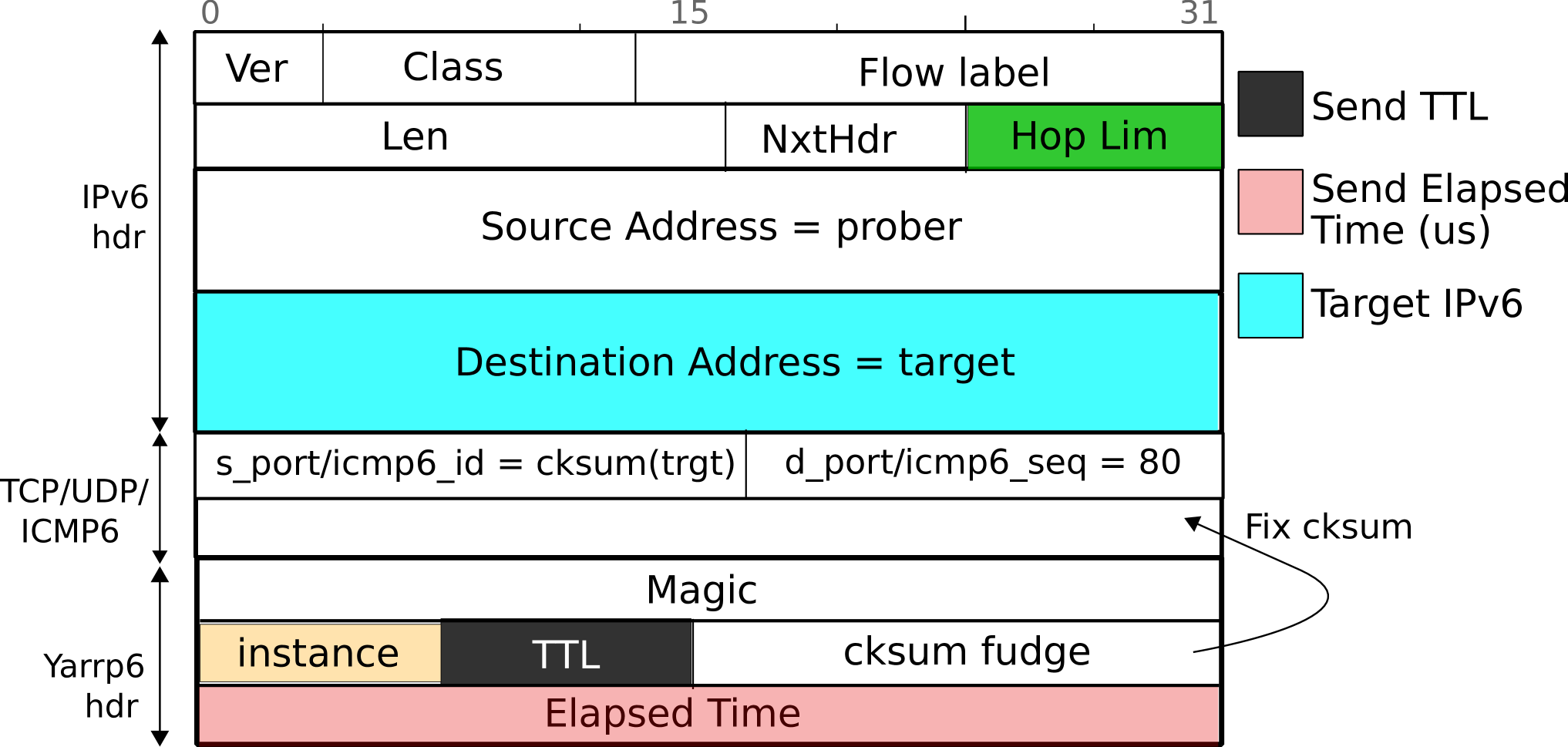
Figure 4. Yarrp6 state: a 12B application payload carries state and corrects the checksum such that the IPv6 and transport headers remain per-target constant.

Figure 4 depicts Yarrp6 state encoding within the probes it sends. After the IPv6 and transport headers is the Yarrp6 payload of 12B. The Yarrp6 payload consists of a 4B magic number and 1B instance ID to ensure that received ICMPv6 packets are indeed responses to Yarrp6 probes, and for the running instance. A single byte encodes the originating TTL (“hop limit”). Four bytes encode the probe’s timestamp to permit round-trip-time (RTT) computation.

Similar to IPv4 paths, Almeida et al. find load balancing prevalent on IPv6 paths they sample (Almeida et al., 2017). We therefore wish to ensure that the packet headers remain constant and accommodate load balanced paths, however the transport checksum will be different for each probe as the TTL and timestamp in the Yarrp6 payload changes. While the transport checksum is not typically used for load-balancing TCP and UDP flows, the ICMPv6 checksum is employed in per-flow load balancing. We therefore include 2B of “fudge” within the Yarrp6 payload in order to ensure that the transport checksum also remains constant. Finally, we compute a 2B Internet checksum over the IPv6 target address and, depending on the transport protocol selected, use it for the TCP or UDP source port or ICMPv6 identifier. This checksum permits detection of modifications to the IPv6 target address, e.g., due to middleboxes.

Fill Mode. A consequence of stateless operation is that Yarrp cannot stop probing when it reaches its destination, or encounters several unresponsive hops in a row (the so-called “gap-limit”) (Beverly, 2016). Instead, the user must select the probe TTL range a priori, potentially missing hops if the maximum TTL is smaller than the path length, or wasting probes if the maximum TTL is too large. To accommodate this tension, we add to Yarrp6 a “fill mode.”

Let the user-selected, initial maximum probing TTL be $m$. In fill mode, if Yarrp6 receives a response for a probe sent with hop limit $h$ where $h\geq m$, it immediately sends a new probe toward the destination with a hop limit of $h+1$. While these additional probes are not randomized, fills are uncommon and occur at the tail of the path where the effect of sequential probing has the least impact. We explore tuning of Yarrp6 parameters, including fill mode, next.

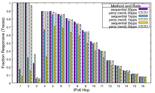
(a) Vantage: US-EDU-3

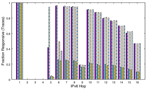
(b) Vantage: US-EDU-2

Figure 5. Trial Results: Relationship between probing strategy, rate, and per-hop responsiveness at two vantage points. While ICMPv6 rate-limiting is clearly evident, randomly permuting the probing order universally improves responsiveness.

4.2. Tuning

In addition to selecting vantage points and targets, active topology discovery requires choosing the probing protocol, maximum TTL, speed, and other parameters. This section explores these parameters to better understand the tradeoffs and to guide our probing strategy.

An evaluation metric we employ is the number of discovered “interface addresses.” Henceforth, we define an interface address to be a unique IPv6 source address of received ICMPv6 messages, and do not attempt to correlate these with interfaces or among routers. In particular, a packet forwarder (e.g., router) has multiple interfaces, including virtual loopbacks, and each interface can have multiple addresses. While (Conta et al., 2006) specifies that nodes should choose a unicast IPv6 source address for ICMPv6 packets according to the packet’s destination, other behaviors may exist.

Protocol. Any IPv6 packet can be used for active topology probing, however the well-known prevalence of middleboxes and firewalls suggests that different packet types, e.g., TCP SYN, TCP ACK, UDP, or ICMPv6, can yield different results depending on whether these are blocked along a path or whether an in-path device maintains connection state. Luckie et al. studied the influence of transport protocol for IPv4 and found that ICMP-Paris reaches the most destinations, while UDP based methods infer the greatest number of IP links (Luckie et al., 2008). CAIDA’s production active topology discovery (CAIDA, 2016, 2018b) utilizes ICMP-Paris for both IPv4 and IPv6.

To the best of our knowledge, there is no published equivalent analysis of the effect of transport protocol on IPv6 active topology discovery. We therefore mounted trial probe campaigns from two of our vantage points on February 1, 2018 using the CAIDA target set. We use the same permutation seed and targets to probe using TCP, UDP, and ICMPv6. To mitigate the possible effects of any rate-limiting, we probed at only 20pps.

On average, we see that probing with ICMPv6 results in $\sim$2.2% and 2.1% more discovered interface addresses than using UDP and TCP respectively. Interestingly, ICMPv6 probes produce on average 13.6% and 24.3% more non-“Time Exceeded” ICMPv6 responses than UDP and TCP respectively, suggesting that these probes are penetrating deeper into the network. Given these observations, we send ICMPv6 probes for the remaining experiments.

Speed. As discussed previously, probing speed has a potentially greater impact on discovery in IPv6 as compared to IPv4 due to mandated rate-limiting. Toward understanding the behavior of various probing techniques and speeds, we mount trial probing campaigns to the CAIDA target set on April 27, 2018 from our vantage points. Figure 5 shows the per-trace fraction of responses received as a function of responding IPv6 hop for speeds of 20, 1000, and 2000 pps, and using two probing strategies: randomized (as implemented in Yarrp6) and sequential (as implemented in scamper (Luckie, 2010)). Scamper running in ICMPv6 Paris mode represents the current state-of-the-art topology probing tool and technique used in production systems. Note that because the number of responsive interface addresses decreases as the hop distance increases, it is necessary to compare the relative performance of Yarrp6 and sequential at different speeds.

We observe markedly different results between sequential and Yarrp6 at speeds above 20pps, especially nearer to the vantage point. For instance, in Figure 5(a), while sequential and Yarrp6 have nearly identical response rates at 20pps, Yarrp6 yields a 100% response rate from the first hop for 1000 and 2000pps as compared to less than 20% and 10% for sequential. Across both vantage points, we observe better performance with Yarrp6 at all hops than achieved with sequential at higher probing rates.

Investigation of timing from packet captures of the two tools shows per-TTL bursty behavior in the sequential prober implementation, a behavior that persists as traces remain synchronized. In addition to Yarrp’s randomization strategy, the rate-limiting effects could also possibly be mitigated with a different transmission behavior, an observation recently made in (Alvarez et al., 2017).

Also of note are the variety of rate-limiting behaviors implemented by routers. For instance, hop 3 of Figure 5(a) and hops 5 and 9 of Figure 5(b) appear to implement more aggressive rate limiting as compared to the other hops. Further, while not pictured, we find one hop near one of our vantage points that only responds with time exceeded messages when ICMPv6 is used as the probe type. Because subsequent hops respond, we conjecture that this behavior is due to some form of state maintenance for security reasons.

Probe order. While sequentially increasing TTL tracing clearly induces ICMPv6 rate limiting, there are a variety of potential probe order strategies that can help mitigate the effects of rate limiting, including Yarrp6’s randomization. Since we first observed the effects of ICMPv6 rate limiting on active topology scans (Gaston and Beverly, 2017), other researchers have recently reported similar findings and explored different probing strategies (Alvarez et al., 2017).

The tree-like structure of the network implies that hops closest to the vantage will experience the most probing traffic, and it follows that we observe these nearby hops exhibiting the most rate-limiting. Thus, a natural strategy to explore is Doubletree (Donnet et al., 2005) which first observed that paths exhibit significant redundancy in their initial hops. Doubletree chooses an intermediate starting TTL and probes forward (increasing TTL) and backward (decreasing TTL) until it receives a response from an interface it has previously observed. Doubletree then fills in missing portions of the path based on previous results.

To better understand Doubletree’s performance relative to ICMPv6 rate limiting, as a trial, we also probe the CAIDA target set from our vantage points at various packet rates using scamper’s Doubletree implementation. While Doubletree induces less rate limiting than traditional traceroute methods, we observe an unexpected effect: when rate limiting causes a hop to be non-responsive, Doubletree continues probing backward in the TTL space. Thus, as the token buckets on the initial hops drain, Doubletree continues to probe them, causing them to remain empty. Notwithstanding this behavior, Doubletree has two fundamental limitations. First, it is necessary to select the intermediate starting TTL, a parameter that must be heuristically estimated and set for each vantage point. Second, using results from previous traces to fill in hops that were not probed can lead to erroneous path inference, either due to violations of destination based routing, as described in (Flach et al., 2012) or path changes. We therefore believe that Yarrp6 provides a compromise between completeness and scalability that is well-suited to Internet-wide IPv6 topology studies.

Finally, we note that Yarrp also includes the ability to employ a similar heuristic as Doubletree where it can maintain state over its local responsive neighborhood (e.g., router interface hops below a configurable TTL). In this mode, Yarrp maintains a per-TTL timestamp of the last time a probe was sent and the last time a probe elicited a new interface address. If no new addresses are discovered within a configurable window of time, Yarrp skips future probes for that TTL. While this work purposefully takes an exhaustive stateless approach, in future research we plan to experiment with Yarrp6’s neighborhood enhancement.

TTL range. As described previously, Yarrp6’s fill mode balances the choice of a maximum probe TTL with discovery rate and volume of probing. Recall that the maximum TTL must be selected in advance as part of the permutation process. Thus, a large maximum TTL will potentially waste probes, while a small maximum TTL will potentially miss hops. Fill mode allows us to select a lower maximum TTL, thereby lowering probing volume, while missing fewer hops.

To quantify this tradeoff, we explore the use of different Yarrp6 maximum TTL values in a final set of trials probing the CAIDA target set on May 2, 2018. In these trials, fill mode continues probing past the maximum TTL so long as responses are received, up to a maximum hop limit of 32. Table 6 shows the number of probes, probes resulting from fills, unique interface addresses discovered, and the interface address yield (addresses discovered per probe). Note that a single non-responsive hop past the maximum TTL will cause fill mode to stop. Thus, we observe that the number of fills for a maximum TTL of four is much less than for a maximum TTL of eight simply because hop five did not respond. Using a maximum TTL of 16 produces the highest yield; we therefore use this for all subsequent campaigns (i.e., results in Section 5) in order to achieve the most efficient use of probing.

Table 6. Fill Mode Trial Results

MaxTTL	Probes	Fills	Int Addrs	Yield %
4	375.6k	96.4k	271	0.1
8	751.2k	213.5k	11.3k	1.2
16	1.5M	251.5k	39.1k	2.2
32	3.0M	0	54.1k	1.8

4.3. Ethical Considerations

Performing large-scale, Internet-wide active measurements requires careful consideration of the experimental methodology to avoid causing harm. First and foremost, we obtained explicit permission from the networks hosting the vantage points in our study. Second, we opt to send ICMPv6 probes as they are relatively innocuous compared to UDP and TCP, are used by the existing Ark and RIPE platforms thereby facilitating direct comparison, and yield the most responses as discussed in Section 4.2. Third, although capable of much higher rates, we run Yarrp6 at 1kpps both to minimize rate-limiting (Section 4.2) and to maintain low network load. (Note that Yarrp’s randomization naturally spreads load.) Fourth, because our goal is to discover IPv6 router addresses, not end hosts, we use the fixed pseudo-random IID for all campaigns, which is unlikely to be that of an active IPv6 host. We show in Section 3.3 that using this IID has negligible effect on topology discovery as compared to the ::1 IID.

Finally, we follow best practices for good Internet citizenship by making an informative web page, along with opt-out instructions, available at the source address of our probes (Durumeric et al., 2013). Over the course of our probing campaigns, we received two opt-out requests with which we immediately complied.

5. Results

Table 7. Results of aggregate Yarrp campaigns run from three vantages, reverse sorted by Int Addrs yield, i.e., sources of ICMPv6 Time-Exceeded messages. Path Offset of EUI-64 Int Addrs is relative to Path Len, 0 being the last Hop Addr on path.

Yarrp6	Agg	Traces	Target	Rtr	Excl	Int	Excl	Int	Excl	Reach	Path Len	EUI-64:		Path Offset
Campaign			Addrs	Int	Int	BGP	Int	ASNs	Int	Target	95th Perc.	Int		5th Perc.
				Addrs	Addrs	Pfxs	BGP		ASNs	ASN	(Median)	Addrs		(Median)
ALL	both	45.8M	12.6M	1.4M	0	9.9k	0	7.1k	0	40%	20 (11)	651.4k	45%	-7 (0)
EU-NET	both	15.0M	12.2M	1.3M	136.0k	9.5k	236	6.9k	110	44%	17 (8)	613.0k	48%	-11 (0)
US-EDU-1	both	15.4M	12.6M	1.3M	84.9k	9.4k	75	6.8k	31	43%	19 (10)	602.7k	48%	-9 (0)
US-EDU-2	both	15.4M	12.6M	881.4k	20.7k	7.4k	148	5.5k	76	33%	21 (15)	540.6k	61%	-2 (0)
cdn k32	z64	9.6M	3.2M	756.6k	534.2k	2.0k	33	1.2k	8	52%	18 (12)	297.2k	39%	0 (0)
tum	z64	6.2M	2.1M	582.4k	364.7k	7.9k	98	6.0k	58	63%	19 (12)	311.2k	53%	-3 (0)
cdn k32	z48	1.6M	524.2k	203.7k	9.6k	1.8k	4	1.2k	2	70%	19 (12)	79.8k	39%	0 (0)
fdns	z64	2.2M	746.9k	185.2k	9.4k	6.2k	5	5.0k	2	48%	19 (10)	15.4k	8%	-1 (0)
dnsdb	z64	698.6k	233.0k	154.0k	23.2k	7.8k	176	6.0k	106	55%	20 (13)	10.1k	7%	-5 (0)
6gen	z64	13.4M	4.5M	126.4k	46.9k	7.1k	174	5.2k	58	27%	31 (12)	24.8k	20%	-18 (0)
tum	z48	1.1M	362.7k	118.3k	2.1k	6.6k	6	5.0k	2	41%	18 (9)	11.6k	10%	-3 (0)
cdn k256	z64	1.2M	396.7k	116.9k	3.4k	1.2k	0	639	0	51%	18 (11)	28.5k	24%	0 (0)
cdn k256	z48	487.1k	162.4k	89.7k	428	1.1k	0	637	0	69%	18 (12)	19.5k	22%	0 (0)
fdns	z48	673.3k	228.7k	88.5k	551	4.8k	0	4.0k	0	29%	18 (6)	4.2k	5%	-8 (0)
dnsdb	z48	281.3k	93.8k	87.9k	662	6.4k	4	5.0k	1	49%	21 (12)	5.5k	6%	-7 (0)
6gen	z48	4.3M	1.4M	69.4k	2.0k	6.5k	40	4.9k	25	16%	32 (12)	3.5k	5%	-19 (-3)
caida	z64	314.7k	105.2k	60.9k	398	6.3k	11	4.8k	5	26%	31 (12)	428	1%	-20 (-4)
caida	z48	234.3k	78.3k	57.7k	92	6.1k	2	4.7k	1	25%	29 (12)	370	1%	-20 (-3)
fiebig	z64	2.8M	1.0M	54.2k	9.6k	3.3k	57	2.8k	49	24%	17 (5)	1.3k	2%	-15 (-3)
fiebig	z48	270.3k	102.2k	22.1k	63	2.7k	0	2.3k	0	11%	17 (4)	177	1%	-17 (-2)

We present the following results: (i) an analysis of the power of the target sets to yield interface addresses in Yarrp6 campaigns; (ii) comparisons of Yarrp6 results to other probers performing similar and different trace campaigns; (iii) detailed results of high-frequency Yarrp6 campaigns launched from three vantage machines each with 18 different target sets (54 in total) on May 14, 2018 and summarized in Figure 6 and Table 7. The top line in the table is the combined result across all three vantages and all campaigns per vantage.

5.1. Topology

In terms of overall discovery, the two best performing target sets are cdn-k32 and tum. Not only do they produce the largest absolute numbers of interfaces, they continue to reveal new addresses throughout the entire probing duration. As shown in Table 7, they are largely complementary and contribute the two largest shares of interfaces exclusively discovered by single target sets.

Figure 6 lets us compare the fraction of total traces performed for each target set by features of the router addresses discovered as a result of those traces. In the small axes on the right of the figure, we isolate just the fraction of exclusive BGP prefixes, and exclusive ASNs for each set, since that is obscured by the shared portion on the main figure.

Rightmost in Table 7, as with the seeds in Section 3, we used addr6 to classify the resulting interface addresses discovered across all trace campaigns. Surprisingly, we find many EUI-64 addresses, 651.4k or 45% of all interface addresses. These are labeled “EUI-64: Int Addrs” in Table 7, most prominently yielded by the tum (53% EUI-64 results) and cdn-k32 (39% EUI-64 results) campaigns. The accompanying percentage shows the proportion of EUI-64 interface addresses within each campaign. Of these EUI-64 router addresses, 59% are from one of just two manufacturers; 99.9% of each of those address are in just two ISP networks, each in different countries. In both cases, WWW content suggests they are Customer Premises Equipment (CPE) routers in ostensibly large, homogeneous IPv6 deployments. Offering further evidence, the last column labeled ”EUI-64: Path Offset” explores the distribution hop positions for EUI-64 interface addresses, as a negative offset from end of path. In all CDN campaigns, we see the 5th percentile and median are 0, meaning 95% of their EUI-64 addresses are the last hop on path. For the TUM campaigns, 50% of their EUI-64 addresses are the last hop on path (median is 0) while 95% are one of the last 3 hops (5th percentile is -3). This topological difference is presumably the result of increased heterogeneity of TUM versus CDN targets.

It is not a coincidence that these two target sets also have highest overall yield and highest yield of exclusive interface addresses (as seen in the “Excl Int Addrs” column). This is due, in large part, to elicited ICMPv6 responses from these CPE routers, one target set yielding one manufacturer’s routers in one ISP’s, and the other ISP containing a different router manufacturer.

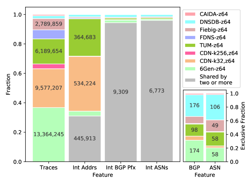
Figure 6. Selected Result Features of Yarrp Campaigns (corresponding to Table 7).

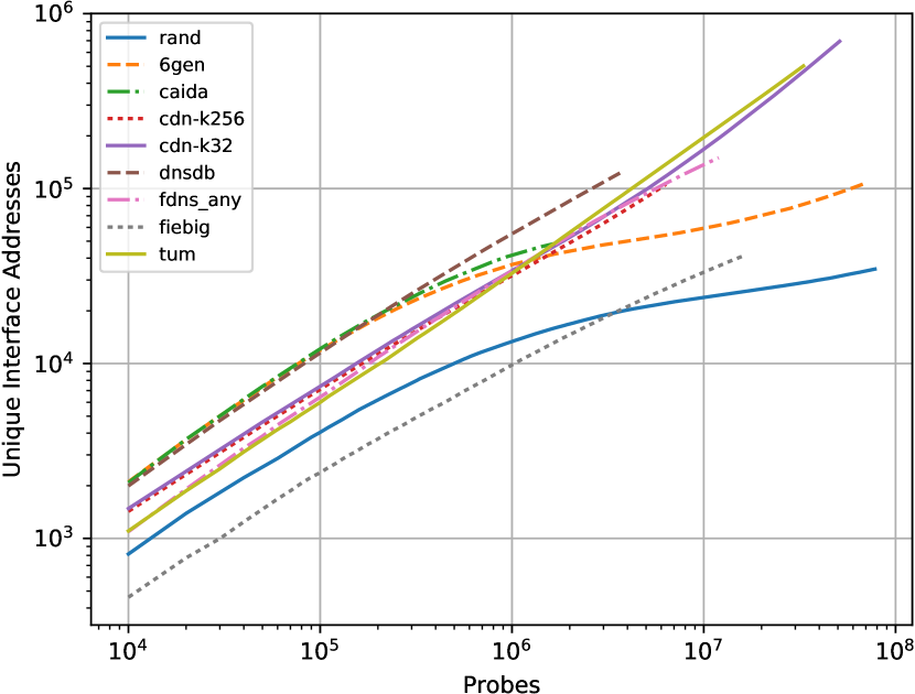
Figure 7. Address discovery power per z64 target set vs. probe packets emitted (from EU-NET vantage in Table 7).

5.2. Target Sets Power

Central to our study is evaluating trace target strategies to not only maximize topological discovery, but also efficiency within an address space too large to be exhaustively probed. In Figure 7, we examine the relationship between each z64 target set’s count of interface addresses discovered via probing from the EU-NET vantage point, and the number of probe packets required. We observe qualitatively similar results from the other vantage points, and choose to focus on the EU-NET results due to space constraints.

The current state-of-the-art strategy, employed by both CAIDA and RIPE for their production IPv6 mapping, of tracing to the ::1 address (plus a random address in CAIDA’s case) within routed IPv6 BGP prefixes performs best in the initial stages of the probing, but suffers a noticeable flattening in discovery past 300k packets (note the log-log plot scale). CAIDA’s discovery peaks at fewer than 100k interfaces after $\approx$2M probes as it exhausts the target set. This dichotomy of performing well initially, but falling well short of the absolute number of interfaces discovered via other target sets, illustrates that this BGP-based strategy provides breadth, but lacks the specificity to discover IPv6 subnetting where significant topology exists in depth.

As a second baseline of a BGP-informed strategy, we probe randomly generated IPv6 addresses that are routable. Unsurprisingly, this unguided target selection performs poorly with a precipitous drop in newly discovered interfaces after $\sim$1M probes. However, random outperforms Fiebig prior to this point, largely due to its high degree of clustering (evident in the DPL of Figure 3). Similarly, the 6gen target set provides a high interface yield at the onset of probing, but flattens past 1M probes. In fact, the shape of the 6gen curve closely mirrors random, but with a fixed positive offset.

In contrast, the overall discovery rate is higher and linear for the tum and cdn-k32 synthesized target lists, implying that these provide the most power. Although they have similar discovery yields, cdn-k32 finds $\sim$200k more addresses from this vantage.

5.3. Validation

As with similar Internet-wide active measurement studies, validation of our method is complicated by limited availability of ground truth and by limited seed address collections, in part, both due to privacy concerns. To place our results in context, we therefore consider our discovered IPv6 topologies relative to those available from production IPv6 active traceroute systems, namely CAIDA’s Ark (CAIDA, 2018b) and RIPE Atlas (RIPE NCC, 2018). For both, we gather the complete set of traceroute results for May 18, 2018 available from each vantage point. Both Ark and Atlas are global platforms, with vantages in different regions and networks. While Ark had 65 IPv6-capable vantages at the time of writing, Atlas had 4,333.

Within the 24 hour period, Atlas probed 34.3k unique targets and discovered 103.8k unique interfaces, while Ark issued traces to 349k targets which revealed 126.8k interfaces. Notably, while Ark used 6.9M traces, our methodology discovers $\sim$1.3M interfaces – an order of magnitude more – with only approximately twice the number of traces.

We further compared our results to those of a proprietary prober that regularly performs millions of traces per day  (Alvarez et al., 2017). With that prober, the cdn-k32-z64-fixediid target set was traced separately on May 3, 2018, i.e., emitting TTL-limited probes toward active WWW client address space. In contrast to Yarrp6, this prober is stateful, like traceroute, and operates by distributing its workload of traces across a set of machines, here, from one physical and topological location to make comparison reasonable. Results show the interface address yield difference was within 1.1%, and other metrics were similar; it is plausible that vantage connectivity and system resources are responsible for the difference.

Lastly, in Table 7, note there is some variation in Yarrp6 results by vantage, despite launching the same campaigns. While EU-NET and US-EDU-1 show similar yield, $\sim$1.3M interface addresses, US-EDU-2 has lower yield, $\sim$881k, despite having performed just as many traces. Our hypothesis is that this vantage is unusual in that its on-premise path is longer (as seen in Figure 5(b) and median path length in 7) and thus may warrant a higher TTL value (per Section 4.2).

6. Subnet Discovery

Having collected voluminous trace results, we turn our attention to topological inference from the results. We employ two techniques to infer subnet boundaries. The first one is based on path divergence observed in traces from prior work (with IPv4), while the second relies on the ubiquitous delegating of /64 prefixes as the most-specific subnets at the Internet’s periphery and thus is IPv6-specific.

Path divergence-based discovery. Inspired by Lee et al. (Lee and Spring, 2016), we discover IPv6 subnets based on path divergence detected in the paths traversed in our trace campaigns. However, IPv6 requires different premises. First, our goal is to infer heterogeneous IPv6 prefixes by splitting subnets, starting with known BGP prefixes, into smaller ones based on divergent hops; whereas subnets are coalesced to identify homogeneous IPv4 prefixes in (Lee and Spring, 2016). Next, there is no canonical equivalent of /24 in IPv6 space due to the freedom afforded network operators by generous address allotments and many transition and feature-based address assignment options.

As in Lee’s work, the keys to the technique are twofold. First, traced paths from one or more vantages to two different target addresses are compared to (a) identify a significant converging subpath (a substring, composed of router hop addresses, that is common to both traced paths) and (b) identify a subsequent significant diverging subpath. By “significant” we mean we are willing to assume that the divergence, in context of the convergence prior, indicates that the two addresses belong to different subnets. We call the converging subpath by the name “last common subpath” (LCS) and refer to the diverging path tails by the name “divergent suffixes” (DS). The second key to the technique is that, once two addresses are assumed to be in different prefixes, we calculate those two addresses’ “discriminating prefix length” (DPL), introduced in Section 3.4.1. Given that we take them to be in different subnets, we know that the first $n$ bits of each address, where $n$ is the DPL, must also be the first $n$ bits of each subnet’s base address and, therefore, the subnet’s prefix length must be at least $n$.

Our implementation, discoverByPathDiv, classifies sets of IPv6 traced paths as divergent (or not) according to these parameters:

• The LCS must have minimum length: $c=2$.

• The LCS must have $C$ hop(s) having an ASN matching the target’s ASN: $C=1$.

• Missing hop addresses are not allowed in the LCS.

• The last hop’s ASN must not match the vantage’s ASN: $A=1$.

• The DS must have minimum length: $s=1$.

• The DS must have $S$ hop(s) whose ASN match the target’s: $S=1$.

• No DS can have zero length: $z=0$.

• The target ASN for each path pair must match: $T=1$.

In this way, our implementation (with these numerous parameters) can be made restrictive about the paths it accepts as evidence of significant path divergence and, therefore, conservative in subnet discovery. We tested even more conservative parameter values, e.g., a higher DS minimum length $s=2$, but path divergences ostensibly due to traffic engineering and load-balancing occurred too near the last hop, as reported also with IPv4 in prior works.

There are additional complications. For instance, (a) IPv6 networks exist that use many ASNs simultaneously, e.g., one originating routes to the BGP prefix(es) covering router addresses and another originating routes for the prefix(es) covering their customer’s (target) addresses. To avoid these failing to meet our path and target ASN requirements, we augment the BGP information with collections of “equivalent” ASNs, identified by operational experience and expert knowledge, e.g., of ISP acquisitions or mergers, considering them equal even though they are distinct numbers. Also, (b) since it is not necessary for networks to globally advertise routes to prefixes covering their routers’ addresses (since routers only need to communicate in LANs or point-to-point links to each other), IPv6 networks also exist that use router addresses not covered in the BGP. To avoid having this violate our path and target ASN requirements, we augment the BGP information with some prefixes that are in Regional Internet Registries but not the global BGP. This is especially important for IPv6 where a small number of very large networks, e.g., Comcast and Charter Spectrum, respectively, present these ASN and IP prefix record keeping challenges.

/64 Discovery. Our second subnet-related topology discovery technique is a simpler one, specific to the IPv6 Internet which typically has /64 subnets at its edge. This scheme is very common since it is required by popular IPv6 address assignment techniques such as SLAAC (Stateless Address Auto-configuration) and SLAAC with temporary privacy extensions (also known as “privacy addresses”) in which every IPv6 host address has an interface identifier (IID) comprising the low 64 bits and a network (subnet) identifier comprising the high 64 bits.

It is often the case that TTL-limited probes to some target address never elicit an ICMP or ICMPv6 response with the target address as its source. This leaves the analyst not knowing whether the resulting path reached the router nearest the target or not, making it hard to make assertions on even simple metrics like the diameter of the Internet (as measured in router hops). To overcome this problem of determining where exactly that last hop is in the topology, we leverage the fact, learned from prior active measurement studies, that many IPv6 routers have the IID value :0000:0000:0000:0001 (canonically displayed as ::1 with zero compression) in the source address used to generate ICMPv6 error messages such as Time-Exceeded (Gray, 2015), e.g., routers serving as the gateway for hosts having address in the subnet for that LAN. Certainly not all IPv6 routers do this, but it is common and is not unlike the practice with IPv4 of, e.g., using 192.168.0.1 as the router gateway address for the 192.168.0.0/24 subnet. When we see a last hop ending in ::1 that has the high 64-bits matching the target address, we assume that the probe elicited a response from the gateway router for the target’s LAN, and thus completed. This is a valuable inference in at least two ways: (a) it allows us to assume this trace reached a unique /64 subnet and thus the target address must be in a different subnet than another target address that, likewise, has a last hop in a different /64 covering prefix, thereby enabling divergence-based discovery; (b) it can help us infer reachability, access control, and firewalling policies that limit results in active measurement campaigns, e.g., to assess vulnerabilities or to discover topological characteristics.

We added this second technique to discoverByPathDiv and call it the “Identity Association (IA) Hack” because it can be leveraged to reverse-engineer the IP address identity (prefix) delegated to a customer by an ISP. This is is an important capability for privacy-minded Internet operation if we wish to guarantee some level of anonymity in IP addresses (Plonka and Berger, 2017); we are pursuing this as future work.

Candidate Subnet Results. We refer to our results as “candidates” because our method determines a lower bound on a subnet’s prefix length. This bound is set based on the highest DPL of a target address ostensibly within the subnet and another ostensibly without, i.e., where the traces show paths to those targets diverged. Thus, a candidate subnet length means that we’ve discovered a subnet having a prefix length of at least that reported.

(a) Distribution of minimum subnet prefix lengths

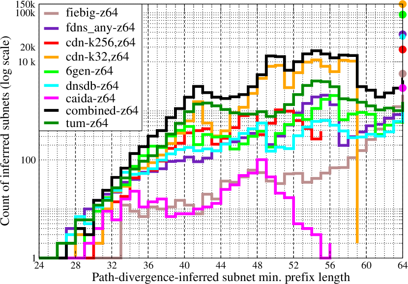
(b) Counts of subnets by prefix length

Figure 8. Subnets inferred by path divergence

Examining the combination of all 45.8M traces for path divergences, we discovered 172,497 candidate subnets, covered by 1,726 BGP prefixes having 1,013 origin ASNs. Figure 8(a) plots the CDF of those subnets for each target set. This figure shows that target sets power to discover candidate subnets is largely governed by their respective addresses’ DPLs plotted in Figure 3(a). Also note that, although we see improved potential power of the target sets in combination (Figure 3(b)), that improved power is not realized here: the CDFs do not shift right. This may be due to active measurement difficulties, e.g., missing hops on traced paths and our conservative approach which does not allow missing hops on the common subpath before divergence.

Figure 8(b) plots counts of discovered subnets by prefix length per target set and combined. Note there are a few prominences suggesting popular prefix lengths (subnet sizes). Also note that, while some target sets help to discover only subnets less than a particular length, e.g., 59 (cdn-k32) or 55 (cdn-k256), others can help to discover more specific subnets because they contain unaggregated, active /64 prefixes, e.g., from the DNS. The dots plotted directly above 64 on the horizontal axis in Figure 8(b) are the counts where the last hop address was covered by the same /64 prefix as the target address, i.e., the IA Hack. (Combined these total to 1,284,891.)

Subnet Validation. To evaluate these results, first we use ground truth data consisting of a set of 12,447 interior prefixes of major US ISP networks (109 BGP prefixes advertised by 30 origin ASNs) and their respective city-level locations and assume those in different cities are also topologically heterogeneous, i.e., in different subnets such that our method should be able to ascertain, if it is given sufficient traces to target addresses in and near those subnets.

We find, that we’ve performed 386,579 traces from each vantage to target addresses covered by 5,839 (47%) of the subnets in truth data. Of those, our algorithm discovered 109 subnets exactly as in the truth data, i.e., having the same base addresses and prefix lengths: 107 /40 prefixes and 2 /64 prefixes. However, because these ground truth subnets are intermediate (in between advertised BGP prefixes and LAN subnets) or “distribution” subnets, we shouldn’t expect many exact matches as our method may have discovered more-specific subnets. Indeed we find that we’ve discovered more specific candidates within 3,871 (66%) of those ground truth prefixes.

To deal with this complication, we re-run our algorithm on a subset of traces selected by stratified sampling, i.e., we choose only one trace to one target address in each ground truth subnet. This intentionally reduces the fidelity of our technique by lowering the target addresses’ DPLs, thus limiting discovery to subnets no more-specific than those in the truth data. With this sampled subset of traces our algorithm yields 914 candidate subnets (18%), 395 (43%) of which exactly match the truth data. Of the non-matching results, 52% have a prefix length that is one bit short and 20% are short by two. Improving this prefix length approximation by lower bound necessitates additional traces to targets with higher DPL. As such, we merely claim these discovered subnet results are plausible based on modest coincidence with ground truth and that stratified sampling is a possible way the technique can be tuned to discover hierarchical subnets.

Attempting to further evaluate subnet discovery results, we examine two universities’ subnet address plans that were shared publicly. For both universities, the entirety of each of their active IPv6 address spaces is covered by just one subnet in our results, having prefix lengths of 41 and 39, respectively. Investigation shows that the anonymization method employed (Plonka and Berger, 2017), e.g., for cdn-k32, kept us from probing targets in these networks ostensibly having too few simultaneously active IPv6 WWW clients. That is, for privacy reasons, no target addresses with sufficiently high DPL were probed to discern more-specific subnets.

7. Discussion and Future Work

In this work, we seek to advance the state-of-the-art in Internet-wide IPv6 active topology mapping. We collect seeds and synthesize targets from a number of sources using a three-step process. Next, to facilitate large-scale IPv6 topology mapping, we emit traceroutes from three vantage points to the targets using a modified version of Yarrp (Yarrp6). Along the way, we investigate the use of various target selection methods and parameters (e.g., maximum TTL, probing speed, etc.) that elicit the most IPv6 topological information. Our investigations provide breadth across networks, depth to discover subnetting, and speed. More specifically, we discover over 1.3M IPv6 interface addresses, which is an order of magnitude more compared to the state-of-the-art mapping systems.

7.1. Security & Privacy

Our results led us to consider security concerns specific to IPv6 topology mapping. Due in part to the address length, IPv6 addresses can contain sensitive information that makes the active IPv6 address space easier to scan or probe, and likely more vulnerable to malicious exploits (Gont and Chown, 2016). For example, our probe campaigns elicited ICMPv6 “Time Exceeded” responses from many sources having IEEE MAC-based EUI-64 addresses. These IIDs ostensibly embed Ethernet addresses, exposing the manufacturer or model of a router (Martin et al., 2016) , and, perhaps, its operating system. RFC 7721 (Cooper et al., 2016) notes that these IEEE-identifier-based IIDs make attacks possible, e.g., address scanning and device exploits. Likewise, we received “Time Exceeded” messages from many addresses covered by the same /64 prefix as a target address, i.e., routers ostensibly collocated, e.g., in a LAN, with hosts. The community should carefully consider the implications of these router-addressing practices as a router’s source address, e.g., when sending ICMPv6 error messages, can disclose details that users may prefer to remain private.

Therefore, we release datasets with restrictions. The public data, available at (Beverly and Rohrer, 2018), contains seeds and targets. The complete data and results will be available to researchers at (DHS, 2018) with restricted distribution. However, we note that our methodology is reproducible using publicly-available seed datasets and freely-available probe utilities. The resulting addresses and subnets discovered or inferred likely extend the attack surface already discernible via hitlists.

7.2. Future Work

Based on these encouraging results, we plan to leverage our methodology across a large number of vantages and time to provide even greater scope and coverage. Further, we plan to perform alias resolution, e.g., (Luckie et al., 2013), to produce router-level topologies and facilitate comparative graph analyses between IPv4 and IPv6.

Finally, our subnet discovery results show that it is sometimes feasible to remotely determine likely IPv6 prefix assigned to a single user or subscriber. In DHCPv6 prefix delegation this is referred to as Identity Association (IA), and prefix lengths can vary according to the services offered and hints offered by a router to which a prefix is delegated, e.g., on the customer premises. We plan to run additional measurement campaigns to comprehensively assess this capability, with the hope that it might inform IP address anonymization by aggregation, to provide a known level of client privacy.

References

- (1)
- rou (2016) 2016. University of Oregon RouteViews. http://www.routeviews.org.
- Almeida et al. (2017) Rafael Almeida, Osvaldo Fonseca, Elverton Fazzion, Dorgival Guedes, Wagner Meira, and Ítalo Cunha. 2017. A Characterization of Load Balancing on the IPv6 Internet. In Conference on Passive and Active Network Measurement.
- Alvarez et al. (2017) Pablo Alvarez, Florin Oprea, and John Rula. 2017. Rate-limiting of IPv6 Traceroutes is Widespread: Measurements and Mitigations. https://datatracker.ietf.org/meeting/99/proceedings#maprg. Measurement and Analysis for Protocols Research Group (MAPRG), IETF 99 Proceedings.
- Augustin et al. (2006) Brice Augustin, Xavier Cuvellier, Benjamin Orgogozo, Fabien Viger, Timur Friedman, Matthieu Latapy, Clémence Magnien, and Renata Teixeira. 2006. Avoiding Traceroute Anomalies with Paris Traceroute. In Proceedings of the ACM Internet Measurement Conference (IMC).
- Beverly (2016) Robert Beverly. 2016. Yarrp’ing the Internet: Randomized High-Speed Active Topology Discovery. In Proceedings of the ACM Internet Measurement Conference (IMC).
- Beverly et al. (2010) Robert Beverly, Arthur Berger, and Geoffrey G. Xie. 2010. Primitives for Active Internet Topology Mapping: Toward High-Frequency Characterization. In Proceedings of the ACM Internet Measurement Conference (IMC).
- Beverly and Rohrer (2018) Robert Beverly and Justin P. Rohrer. 2018. Yarrp6 Beholder Datasets. https://www.cmand.org/yarrp/ipv6/.
- Borgolte et al. (2018) Kevin Borgolte, Shuang Hao, Tobias Fiebig, and Giovanni Vigna. 2018. Enumerating Active IPv6 Hosts for Large-scale Security Scans via DNSSEC-signed Reverse Zones. In Proceedings of 39th IEEE Symposium on Security and Privacy.
- CAIDA (2016) CAIDA. 2016. The CAIDA UCSD IPv4 Routed /24 Topology Dataset. http://www.caida.org/data/active/ipv4_routed_24_topology_dataset.xml.
- CAIDA (2018a) CAIDA. 2018a. The CAIDA Internet Topology Data Kit. http://www.caida.org/data/internet-topology-data-kit.
- CAIDA (2018b) CAIDA. 2018b. The CAIDA UCSD IPv6 Topology Dataset. http://www.caida.org/data/active/ipv6_allpref_topology_dataset.xml.
- Collins et al. (2007) M Patrick Collins, Timothy J Shimeall, Sidney Faber, Jeff Janies, Rhiannon Weaver, Markus De Shon, and Joseph Kadane. 2007. Using Uncleanliness to Predict Future Botnet Addresses. In Proceedings of the ACM Internet Measurement Conference (IMC).
- Conta et al. (2006) A. Conta, S. Deering, and M. Gupta. 2006. Internet Control Message Protocol (ICMPv6) for the Internet Protocol Version 6 (IPv6) Specification. RFC 4443. http://www.ietf.org/rfc/rfc4443.txt
- Cooper et al. (2016) A. Cooper, F. Gont, and D. Thaler. 2016. Security and Privacy Considerations for IPv6 Address Generation Mechanisms. RFC 7721 (Informational). http://www.ietf.org/rfc/rfc7721.txt
- Czyz et al. (2014) Jakub Czyz, Mark Allman, Jing Zhang, Scott Iekel-Johnson, Eric Osterweil, and Michael Bailey. 2014. Measuring IPv6 Adoption. In ACM SIGCOMM.
- Czyz et al. (2016) J. Czyz, M. Luckie, M. Allman, and M. Bailey. 2016. Don’t Forget to Lock the Back Door! A Characterization of IPv6 Network Security Policy. In Network and Distributed Systems Security (NDSS).
- Dainotti et al. (2013) Alberto Dainotti, Karyn Benson, Alistair King, Michael Kallitsis, Eduard Glatz, Xenofontas Dimitropoulos, et al. 2013. Estimating Internet Address Space Usage through Passive Measurements. ACM SIGCOMM CCR (2013).
- Dhamdhere et al. (2012) A. Dhamdhere, M. Luckie, B. Huffaker, k. claffy, A. Elmokashfi, and E. Aben. 2012. Measuring the Deployment of IPv6: Topology, Routing and Performance. In Proceedings of the ACM Internet Measurement Conference (IMC).
- DHS (2018) DHS. 2018. IMPACT Cyber Trust. https://www.impactcybertrust.org/.
- Donnet et al. (2005) Benoit Donnet, Philippe Raoult, Timur Friedman, and Mark Crovella. 2005. Efficient Algorithms for Large-Scale Topology Discovery. ACM SIGMETRICS Performance Evaluation Review 33, 1 (2005).
- Durumeric et al. (2013) Zakir Durumeric, Eric Wustrow, and J Alex Halderman. 2013. ZMap: Fast Internet-wide Scanning and Its Security Applications.. In USENIX Security.
- Fiebig et al. (2017) Tobias Fiebig, Kevin Borgolte, Shuang Hao, Christopher Kruegel, and Giovanni Vigna. 2017. Something From Nothing (There): Collecting Global IPv6 Datasets From DNS. In Proceedings of the 18th Passive and Active Measurement Conference.
- Flach et al. (2012) Tobias Flach, Ethan Katz-Bassett, and Ramesh Govindan. 2012. Quantifying Violations of Destination-based Forwarding on the Internet. In Proceedings of the ACM Internet Measurement Conference (IMC).
- Foremski et al. (2016) Pawel Foremski, David Plonka, and Arthur Berger. 2016. Entropy/IP: Uncovering Structure in IPv6 Addresses. In Proceedings of the ACM Internet Measurement Conference (IMC).
- Gasser et al. (2016) Oliver Gasser, Quirin Scheitle, Sebastian Gebhard, and Georg Carle. 2016. Scanning the IPv6 Internet: Towards a Comprehensive Hitlist. In Workshop on Traffic Monitoring and Analysis.
- Gasser et al. (2018) Oliver Gasser, Quirin Scheitle, Qasim Lone, Maciej Korczynski, Stephen D. Strowes, Luuk Hendriks, and Georg Carle. 2018. Clusters in the Expanse: Understanding and Unbiasing IPv6 Hitlists. In Proceedings of the ACM Internet Measurement Conference (IMC).
- Gaston and Beverly (2017) Eric Gaston and Robert Beverly. 2017. Yarrp’ing the IPv6 Internet. https://www.caida.org/workshops/aims/1703/slides/aims1703_egaston.pdf.
- Gaston (2017) Erik W. Gaston. 2017. High-frequency mapping of the IPv6 Internet using Yarrp. Master’s thesis. Naval Postgraduate School. http://hdl.handle.net/10945/52982.
- Gont and Chown (2016) F. Gont and T. Chown. 2016. Network Reconnaissance in IPv6 Networks. RFC 7707 (Informational). http://www.ietf.org/rfc/rfc7707.txt
- Google (2018) Google. 2018. IPv6 Adoption Statistics. https://www.google.com/intl/en/ipv6/statistics.html.
- Govindan and Tangmunarunkit (2000) Ramesh Govindan and Hongsuda Tangmunarunkit. 2000. Heuristics for Internet map discovery. In Proceedings of IEEE INFOCOM, Vol. 3.
- Gray (2015) Matthew D. Gray. 2015. Discovery of IPv6 router interface addresses via heuristic methods. Master’s thesis. Naval Postgraduate School. http://hdl.handle.net/10945/47265.
- Hinden and Deering (2006) R. Hinden and S. Deering. 2006. IP Version 6 Addressing Architecture. RFC 4291 (Draft Standard).
- Huston (2018) Geoff Huston. 2018. BGP Routing Table Analysis. https://bgp.potaroo.net/index-v6.html.
- k. claffy et al. (2009) k. claffy, Young Hyun, Ken Keys, and Maria Fomenkov. 2009. Internet Mapping: from Art to Science. In IEEE Cybersecurity Applications for Homeland Security.
- Kahn et al. (2018) Z. Kahn, J. Brzozowski, and R. White. 2018. Requirements for IPv6 Routers. Internet-Draft (Informational). https://tools.ietf.org/html/draft-ietf-v6ops-ipv6rtr-reqs
- Kalafut et al. (2010) Andrew J Kalafut, Craig A Shue, and Minaxi Gupta. 2010. Malicious Hubs: Detecting Abnormally Malicious Autonomous Systems. In INFOCOM.
- Keys (2010) Ken Keys. 2010. Internet-Scale IP Alias Resolution Techniques. SIGCOMM Comput. Commun. Rev. 40, 1 (2010).
- Kohler et al. (2002) E. Kohler, J. Li, V. Paxson, and S. Shenker. 2002. Observed Structure of Addresses in IP Traffic. In Internet Measurement Workshop.
- Lee and Spring (2016) Youndo Lee and Neil Spring. 2016. Identifying and Aggregating Homogeneous IPv4 /24 Blocks with Hobbit. In Proceedings of the ACM Internet Measurement Conference (IMC).
- Luckie (2010) Matthew Luckie. 2010. Scamper: a Scalable and Extensible Packet Prober for Active Measurement of the Internet. In Proceedings of the ACM Internet Measurement Conference (IMC).
- Luckie et al. (2013) Matthew Luckie, Robert Beverly, William Brinkmeyer, and kc claffy. 2013. Speedtrap: Internet-Scale IPv6 Alias Resolution. In Proceedings of the ACM Internet Measurement Conference (IMC).
- Luckie et al. (2008) M. Luckie, Y. Hyun, and B. Huffaker. 2008. Traceroute Probe Method and Forward IP Path Inference. In Proceedings of the ACM Internet Measurement Conference (IMC).
- Malone (2008) David Malone. 2008. Observations of IPv6 Addresses. In Passive and Active Network Measurement, 9th International Conference, (PAM 2008), 2008. Proceedings.
- Martin et al. (2016) Jeremy Martin, Erik C. Rye, and Robert Beverly. 2016. Decomposition of MAC Address Structure for Granular Device Inference. In Proceedings of the 32nd Annual Computer Security Applications Conference (ACSAC).
- Murdock et al. (2017) Austin Murdock, Frank Li, Paul Bramsen, Zakir Durumeric, and Vern Paxson. 2017. Target Generation for Internet-wide IPv6 Scanning. In Proceedings of the ACM Internet Measurement Conference (IMC).
- Padmanabhan et al. (2015) Ramakrishna Padmanabhan, Zhihao Li, Dave Levin, and Neil Spring. 2015. UAv6: Alias Resolution in IPv6 Using Unused Addresses. In Proceedings of Passive and Active Measurement Conference 2015 (PAM 2015).
- Plonka and Berger (2015) David Plonka and Arthur Berger. 2015. Temporal and Spatial Classification of Active IPv6 Addresses. In Proceedings of the ACM Internet Measurement Conference (IMC).
- Plonka and Berger (2017) David Plonka and Arthur W. Berger. 2017. kIP: a Measured Approach to IPv6 Address Anonymization. CoRR abs/1707.03900 (2017). arXiv:1707.03900 http://arxiv.org/abs/1707.03900
- Plonka and Rose (2017) David Plonka and Kyle Rose. 2017. A Continuing Study of the Active IPv6 WWW Client Address Space. https://datatracker.ietf.org/meeting/100/proceedings#maprg. Measurement and Analysis for Protocols Research Group (MAPRG), IETF 100 Proceedings.
- Rapid7 (2018) Rapid7. 2018. Forward DNS datasets. https://scans.io/study/sonar.fdns_v2.
- RIPE NCC (2018) RIPE NCC. 2018. RIPE Atlas. https://atlas.ripe.net/.
- Rohrer et al. (2016) Justin P. Rohrer, Blake LaFever, and Robert Beverly. 2016. Empirical Study of Router IPv6 Interface Address Distributions. IEEE Internet Computing (Aug. 2016).
- Security (2018) Farsight Security. 2018. Passive DNS project. https://www.farsightsecurity.com/technical/passive-dns/.
- SI6 Networks (2016) SI6 Networks. 2016. SI6 Networks’ IPv6 Toolkit. https://github.com/fgont/ipv6toolkit.
- Spring et al. (2002) Neil Spring, Ratul Mahajan, and David Wetherall. 2002. Measuring ISP topologies with Rocketfuel. ACM SIGCOMM Computer Communication Review 32, 4 (2002).
- Syamkumar et al. (2016) Meenakshi Syamkumar, Ramakrishnan Durairajan, and Paul Barford. 2016. Bigfoot: A Geo-based Visualization Methodology for Detecting BGP Threats. In Visualization for Cyber Security (VizSec).
- Ullrich et al. (2015) Johanna Ullrich, Peter Kieseberg, Katharina Krombholz, and Edgar Weippl. 2015. On Reconnaissance with IPv6: a Pattern-Based Scanning Approach. In Availability, Reliability and Security (ARES).
- Zhang et al. (2008) Zheng Zhang, Ying Zhang, Y Charlie Hu, Z Morley Mao, and Randy Bush. 2008. iSPY: Detecting IP Prefix Hijacking on My Own. In ACM SIGCOMM Computer Communication Review.