Stabilising Fulde-Ferrel-Larkin-Ovchinnikov Superfluidity with long-range Interactions in a mixed dimensional Bose-Fermi System

Abstract

We analyse the stability of inhomogeneous superfluid phases in a system consisting of identical fermions confined in two layers that are immersed in a Bose-Einstein condensate (BEC). The fermions in the two layers interact via an induced interaction mediated by the BEC, which gives rise to pairing. We present zero temperature phase diagrams varying the chemical potential difference between the two layers and the range of the induced interaction, and show that there is a large region where an inhomogeneous superfluid phase is the ground state. This region grows with increasing range of the induced interaction and it can be much larger than for a corresponding system with a short range interaction. The range of the interaction is controlled by the healing length of the BEC, which makes the present system a powerful tunable platform to stabilise inhomogeneous superfluid phases. We furthermore analyse the melting of the superfluid phases in the layers via phase fluctuations as described by the Berezinskii-Kosterlitz-Thouless mechanism and show that the normal, homogeneous and inhomogeneous superfluid phases meet in a tricritical point. The superfluid density of the inhomogeneous superfluid phase is reduced by inherent gapless excitations, and we demonstrate that this leads to a significant suppression of the critical temperature as compared to the homogeneous superfluid phase.

I Introduction

The interplay between population imbalance and superfluid pairing has been subject to intense study ever since Fulde and Ferrell (FF) as well as Larkin and Ovchinnikov (LO) predicted that they can co-exist Fulde and Ferrell (1964); Larkin and Ovchinnikov (1965). In condensed matter systems, an external magnetic field leads to a population imbalance between the two electron spin projections, which in general is at odds with superconductivity. FFLO however realised that the superconductor can accommodate some population imbalance at the price of giving the Cooper pairs a non-zero center-of-mass (COM) momentum, thereby forming a spatially inhomogeneous but periodic order parameter with no vortices. The fate of superfluid pairing in the presence of population imbalance is a fundamental question relevant for many systems in nature including cold atoms Chevy and Mora (2010); Radzihovsky and Sheehy (2010); Kinnunen et al. (2018), superconductors Matsuda and Shimahara (2007), and quark matter Casalbuoni and Nardulli (2004); Alford et al. (2008); Anglani et al. (2014). Nevertheless, an unambiguous observation of a FFLO phase is still lacking. A major problem for electronic superconductors is that orbital effects due to the magnetic field lead to the formation of vortices and eventually destroy pairing before any FFLO physics can be observed. One strategy to avoid this problem is to explore low dimensional systems, where orbital effects are suppressed due to the confinement. Indeed, results consistent with a FFLO phase have been reported for quasi-2D organic and heavy fermion superconductors Beyer and Wosnitza (2013); Mayaffre et al. (2014); Bianchi et al. (2003). Theoretical studies have furthermore concluded that the FFLO phase is favored in 2D as compared to 3D Shimahara (1994); Burkhardt and Rainer (1994); Pieri et al. (2007).

Quantum degenerate atomic gases are well suited to investigate FFLO physics, because they do not suffer from orbital effects as the atoms are neutral. In addition, it is relatively straightforward to make low dimensional systems, and signatures of FFLO physics has indeed been observed in a one-dimensional (1D) atomic Fermi gas Liao et al. (2010). There has been a number of investigations of the FFLO phase for 2D atomic gases with a short range interaction Gukelberger et al. (2016); Baarsma and Törmä (2016); Conduit et al. (2008); Radzihovsky and Vishwanath (2009); Wolak et al. (2012); Yin et al. (2014); Sheehy (2015). Recently, it was argued that long range interactions further increases the region of stability of the FFLO phase for a 2D gas of dipolar atoms as compared to a short range interaction Lee et al. (2017).

Here, we investigate how to stabilise FFLO superfluidity using a mixed dimensional system with a tuneable range interaction. The system consists of fermions confined in two layers immersed in a BEC. The induced interaction between the layers mediated by the BEC gives rise to pairing, and we analyse the stability of the corresponding superfluid phases. We show that the zero temperature phase diagram as a function of the chemical potential difference in the two layers and the range of the interaction has a large region, where an inhomogeneous superfluid phase is the ground state. This region grows with increasing range of the interaction and becomes much wider than for a zero range interaction. The interaction range can be tuned by varying the healing length of the BEC. We furthermore investigate the melting of the 2D superfluid phases via the Berezinskii-Kosterlitz-Thouless mechanism. The normal phase, the homogeneous and inhomogeneous superfluid phases are shown to meet in a tricritical point in the phase diagram, which determines the maximum critical temperature of the inhomogeneous superfluid. This maximum temperature is however significantly suppressed compared to the homogeneous superfluid phase, due to inherent gapless excitations, which decrease the superfluid density.

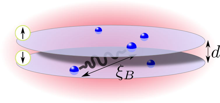
Figure 1: (Color online) A sketch of the considered system. The fermions (blue) are confined in two layers immersed in a three-dimensional BEC (red), with a layer distance $d$. The BEC mediates an interaction between fermions in the two different layers of the Yukawa form, with a range determined by the BEC healing length $\xi_{B}$.

II The Bilayer System

We consider the system illustrated in Fig. 1. Two layers contain fermions of a single species with mass $m$, and they are immersed in a 3D weakly interacting BEC consisting of bosons with mass $m_{B}$ and density $n_{B}$. The distance between the layers is $d$ and the surface density of fermions in each layer is $n_{\sigma}$ with $\sigma=\uparrow,\downarrow$ denoting the two layers. When used in equations, they are taken to mean $\uparrow=+1,\downarrow=-1$, respectively. Occasionally we will also use the notation $\bar{\sigma}$ to mean the opposite layer from $\sigma$. The boson-fermion interaction is short range and characterised by the strength $g=2\pi a_{\text{eff}}/\sqrt{m_{r}m_{B}}$ with $m_{r}=mm_{B}/(m+m_{B})$ the reduced mass, and $a_{\text{eff}}$ the effective 2D-3D scattering length Nishida and Tan (2008). Throughout, this interaction strength is taken to be weak in the sense $k_{F\sigma}a_{\text{eff}}\ll 1$, where $k_{F\sigma}=\sqrt{4\pi n_{\sigma}}$ is the Fermi momentum of layer $\sigma$.

We treat the BEC using zero temperature Bogoliubov theory. This is a good approximation since the critical temperature of the superfluid phases of the fermions is much smaller than the critical temperature of the BEC. The bosonic degrees of freedom can then be integrated out, which yields an effective interaction between the fermions. In the static limit, this interaction is on the Yukawa form, and we end up with an effective Hamiltonian for the fermions in the two layers on the form Heiselberg et al. (2000); Wu and Bruun (2016); Midtgaard et al. (2017)

$$H= H_{\text{kin}}+H_{\text{int}}=\sum_{\mathbf{k},\sigma}\xi_{\mathbf{k}\sigma}c^{\dagger}_{\mathbf{k}\sigma}c_{\mathbf{k}\sigma}$$

$$+\frac{1}{2\mathcal{V}}\sum_{\sigma,\sigma^{\prime}}\sum_{\mathbf{k},\mathbf{k}^{\prime},\mathbf{q}}V_{\sigma\sigma^{\prime}}(\mathbf{q})c^{\dagger}_{\mathbf{k}+\mathbf{q}\sigma}c^{\dagger}_{\mathbf{k}^{\prime}-\mathbf{q}\sigma^{\prime}}c_{\mathbf{k}^{\prime}\sigma^{\prime}}c_{\mathbf{k}\sigma}.$$ (1)

Here, $c^{\dagger}_{\mathbf{k}\sigma}$ creates a fermion in layer $\sigma$ with 2D momentum $\mathbf{k}=(k_{x},k_{y})$, the dispersion in each layer is $\xi_{\mathbf{k}\sigma}=k^{2}/2m-\mu_{\sigma}$ with $\mu_{\sigma}$ the chemical potentials, and $\mathcal{V}$ is the system volume. We define the average chemical potential $\mu=(\mu_{\uparrow}+\mu_{\downarrow})/2$ and the “magnetic field” $h=(\mu_{\downarrow}-\mu_{\uparrow})/2$, so that we can write $\xi_{\mathbf{k}\sigma}=k^{2}/2m-\mu+\sigma\cdot h$. The Yukawa interaction is

$$V_{\sigma\sigma^{\prime}}(\mathbf{q})=-\frac{2g^{2}n_{B}m_{B}}{\sqrt{q^{2}+2/\xi_{B}^{2}}}e^{-\sqrt{k^{2}+2/\xi_{B}^{2}}\cdot|\sigma-\sigma^{\prime}|d/2},$$ (2)

where $\xi_{B}=1/\sqrt{8\pi n_{B}a_{B}}$ is the healing length of the BEC with $a_{B}$ the boson-boson scattering length. The healing length determines the range of the induced interaction as can be seen by Fourier transforming Eq. (2) by to real space giving $V(r)=g^{2}n_{B}m_{B}\pi^{-1}\exp(-\sqrt{2}r/\xi_{B})$ with $r$ the 3D distance between the fermions. It follows that the range of the interaction can be tuned by varying the density $n_{B}$ or the scattering length $a_{B}$ of the surrounding BEC, which turns out to be a key property for the following. We note that retardation effects can be neglected, when the speed of sound in the BEC is much larger than the Fermi velocity in the two planes Wu and Bruun (2016).

III Pairing and Green’s functions

The attractive interaction given by Eq. (2) can lead to Cooper pairing within each layer (intralayer pairing), and between the two layers (interlayer pairing). We recently analysed the competition between intra- and interlayer pairing for the case of equal density in each layer, i.e. for $n_{\uparrow}=n_{\downarrow}$ Midtgaard et al. (2017). For a layer distance $d$ large compared to the range $\xi_{B}$ of the interaction, we found that the ground state is characterised by intralayer $p$-wave pairing, whereas $s$-wave interlayer pairing is stable for smaller $d/\xi_{B}$. In addition, we identified a crossover phase for intermediate $d/\xi_{B}$ where both types of pairing co-exist.

In this paper, we focus on interlayer $s$-wave pairing corresponding to $d/\xi_{B}\lesssim 1$. We shall investigate the case of a non-zero field $h$ giving rise to a population difference between the two layers, and the possibility of FFLO interlayer pairing with non-zero COM momentum. Such interlayer pairing with COM momentum $\mathbf{Q}$ is characterised by the anomalous averages $\langle c_{\mathbf{Q}/2+\mathbf{k}\sigma}c_{\mathbf{Q}/2-\mathbf{k},\bar{\sigma}}\rangle$, which leads us to define the corresponding pairing field

$$\Delta_{\sigma\bar{\sigma}}(\mathbf{k},\mathbf{Q})=\frac{1}{\mathcal{V}}\sum_{\mathbf{k}^{\prime}}V(\mathbf{k}-\mathbf{k}^{\prime})\langle c_{\mathbf{Q}/2+\mathbf{k}^{\prime}\sigma}c_{\mathbf{Q}/2-\mathbf{k}^{\prime},\bar{\sigma}}\rangle.$$ (3)

We have dropped the subscripts on the induced interaction $V(\mathbf{q})$, as it here and in the following refers to the interlayer interaction only, i.e. $V(\mathbf{q})\equiv V_{\sigma\bar{\sigma}}(\mathbf{q})$. The pairing field obeys the Fermi anti-symmetry $\Delta_{\sigma\bar{\sigma}}(\mathbf{k},\mathbf{Q})=-\Delta_{\bar{\sigma}\sigma}(-\mathbf{k},\mathbf{Q})$. In real space, it is on the form

$$\Delta_{\sigma\bar{\sigma}}(\mathbf{r}_{1},\mathbf{r}_{2})= V(\mathbf{r}_{1}-\mathbf{r}_{2})\langle\psi_{\sigma}(\mathbf{r}_{1})\psi_{\bar{\sigma}}(\mathbf{r}_{2})\rangle$$

$$= \frac{1}{\mathcal{V}}\sum_{\mathbf{Q},\mathbf{k}}\Delta_{\sigma\bar{\sigma}}(\mathbf{k},\mathbf{Q})e^{i\mathbf{Q}\cdot{\mathbf{R}}}e^{i\mathbf{k}\cdot{\mathbf{r}}},$$ (4)

where ${\mathbf{R}}=({\mathbf{r}}_{1}+{\mathbf{r}}_{2})/2$ and ${\mathbf{r}}={\mathbf{r}}_{1}-{\mathbf{r}}_{2}$ are the COM and relative coordinates respectively, and $\psi_{\sigma}(\mathbf{r})=\sum_{\mathbf{k}}c_{\mathbf{k}\sigma}\exp(\mathbf{k}\cdot\mathbf{r})$ is the field operator for particles in layer $\sigma$. We note that the pairing field is not translationally symmetric in the FFLO phase, i.e. $\Delta_{\sigma\bar{\sigma}}(\mathbf{r}_{1},\mathbf{r}_{2})\neq\Delta_{\sigma\bar{\sigma}}(\mathbf{r}_{1}-\mathbf{r}_{2})$. The interaction becomes in the mean-field BCS approximation

$$H_{\text{int}}^{\text{MF}}=\sum_{\mathbf{Q},\mathbf{k}}\Delta_{\uparrow\downarrow}(\mathbf{k},\mathbf{Q})c^{\dagger}_{\mathbf{Q}/2-\mathbf{k}\downarrow}c^{\dagger}_{\mathbf{Q}/2+\mathbf{k}\uparrow}+\text{h.c.},$$ (5)

where we include only the pairing channel as we focus on the superfluid instability. The Hartree-Fock terms will in general lead to small effects in the weak coupling regime, which mostly can be accounted for by a renormalisation of the chemical potentials $\mu_{\sigma}$.

All results presented here can be obtained by a direct diagonalisation of the mean-field BCS Hamiltonian $H^{\text{MF}}=H_{0}+H_{\text{int}}^{\text{MF}}$ using a standard Bogoliubov transformation. We however use Green’s functions to analyse the FFLO states, since this formalism naturally allows us to go beyond mean-field theory to include effects such as retardation, if needed in the future. The normal and anomalous Green’s functions for the superfluid phases are defined in the standard way as

$$G_{\sigma}(\mathbf{k},\mathbf{k}^{\prime},\tau) =-\langle T_{\tau}c_{\mathbf{k}\sigma}(\tau)c_{\mathbf{k}^{\prime}\sigma}^{\dagger}(0)\rangle$$

$$F_{\sigma}(\mathbf{k},\mathbf{k}^{\prime},\tau) =-\langle T_{\tau}c_{\mathbf{k}\sigma}(\tau)c_{-\mathbf{k}^{\prime},\bar{\sigma}}(0)\rangle$$

$$F^{\dagger}_{\sigma}(\mathbf{k},\mathbf{k}^{\prime},\tau) =-\langle T_{\tau}c^{\dagger}_{-\mathbf{k},\sigma}(\tau)c_{\mathbf{k}^{\prime}\bar{\sigma}}^{\dagger}(0)\rangle,$$ (6)

where $T_{\tau}$ denotes imaginary-time ordering. Using $H^{\text{MF}}=H_{\text{kin}}+H_{\text{int}}^{\text{MF}}$, the Gor’kov equations for these Green’s functions are straightforwardly derived. They read

$$\left(i\omega_{n}-\xi_{\mathbf{k}\sigma}\right)G_{\sigma}(\mathbf{k},\mathbf{k}^{\prime},\omega_{n}) =\delta_{\mathbf{k},\mathbf{k}^{\prime}}-\sum_{\mathbf{Q}}\Delta_{\sigma\bar{\sigma}}(\mathbf{k}-\mathbf{Q}/2,\mathbf{Q})F^{\dagger}_{\bar{\sigma}}(\mathbf{k}-\mathbf{Q},\mathbf{k}^{\prime},i\omega_{n})$$ (7)

$$\left(i\omega_{n}-\xi_{\mathbf{k}\sigma}\right)F_{\sigma}(\mathbf{k},\mathbf{k}^{\prime},\omega_{n}) =\sum_{\mathbf{Q}}\Delta_{\sigma\bar{\sigma}}(\mathbf{k}-\mathbf{Q}/2,\mathbf{Q})G_{\sigma}(-\mathbf{k}^{\prime},-\mathbf{k}+\mathbf{Q},-i\omega_{n})$$ (8)

$$\left(i\omega_{n}+\xi_{-\mathbf{k},\sigma}\right)F^{\dagger}_{\sigma}(\mathbf{k},\mathbf{k}^{\prime},\omega_{n}) =\sum_{\mathbf{Q}}\Delta^{\ast}_{\sigma\bar{\sigma}}(-\mathbf{k}-\mathbf{Q}/2,\mathbf{Q})G_{\bar{\sigma}}(\mathbf{k}+\mathbf{Q},\mathbf{k}^{\prime},i\omega_{n}),$$ (9)

where we have Fourier transformed to Matsubara frequency space with $\omega_{n}=(2n+1)\pi T$. The self-consistent gap equation is then from (3) and (6)

$$\Delta_{\sigma\bar{\sigma}}(\mathbf{k},\mathbf{Q})=-\frac{T}{\mathcal{V}}\sum_{\mathbf{k}^{\prime},n}V(\mathbf{k}-\mathbf{k}^{\prime})$$

$$\times F_{\sigma}(\mathbf{Q}/2+\mathbf{k}^{\prime}/2,\mathbf{k}^{\prime}-\mathbf{Q}/2,i\omega_{n})e^{-i\omega_{n}0_{+}}.$$ (10)

IV Fulde-Ferrel Superconductivity

The $\mathbf{Q}$ values for which $\Delta_{\sigma\bar{\sigma}}(\mathbf{k},\mathbf{Q})$ is non-zero determines the structure of the order parameter in the superfluid phase. It has been shown that $\Delta_{\sigma\bar{\sigma}}(\mathbf{r}_{1},\mathbf{r}_{2})$ can form very complicated 2D structures corresponding to $\Delta_{\sigma\bar{\sigma}}(\mathbf{k},\mathbf{Q})\neq 0$ for many $\mathbf{Q}$s in Eq. (4) Shimahara (1998); Mora and Combescot (2004). However, the FFLO phase exhibits a second order transition to the normal phase in 2D at an upper critical field $h_{c2}$ Shimahara (1994); Burkhardt and Rainer (1994), and at this transition it is sufficient to consider the case of $\Delta_{\sigma\bar{\sigma}}(\mathbf{k},\mathbf{Q})\neq 0$ only for a single $\mathbf{Q}$ vector. The reason is that any linear combination of the $\Delta_{\sigma\bar{\sigma}}(\mathbf{k},\mathbf{Q})$’s, which are unstable towards pairing, is degenerate at $h_{c2}$, since it is only the non-linear part of the gap equation that determines the optimal combination that minimises the energy.

In the following, we therefore consider the case $\Delta_{\sigma\bar{\sigma}}(\mathbf{k},\mathbf{Q})\neq 0$ only for a single $\mathbf{Q}$. This will give the correct upper critical field $h_{c2}$ for the second order transition between the FFLO and the normal phase. We also expect that it will give a fairly precise value for the lower critical field $h_{c1}$ determining the first order transition between the FFLO and the superfluid phase, since the energy difference between the FFLO phases with various spatial structures is small Shimahara (1998); Mora and Combescot (2004). Our scheme recovers the usual homogenous BCS pairing for $\mathbf{Q}=0$, and it corresponds to a plane wave Fulde-Ferrel (FF) type of pairing when $\mathbf{Q}\neq 0$, as can be seen from Eq. (4). Since we only have one $\mathbf{Q}$ vector, we can simplify the notation for the gap as $\Delta_{\sigma\bar{\sigma}}(\mathbf{k},\mathbf{Q})\to\Delta_{\sigma\bar{\sigma}}(\mathbf{k})$. The Gor’kov equations (7)-(9) are then easily solved giving

$$G_{\sigma}(\mathbf{k},\mathbf{k}^{\prime}i\omega_{n}) =\delta_{\mathbf{k},\mathbf{k}^{\prime}}\left(i\omega_{n}-\xi_{\mathbf{k},\sigma}-\frac{|\Delta_{\sigma\bar{\sigma}}(\mathbf{k}-\mathbf{Q}/2)|^{2}}{i\omega_{n}+\xi_{-\mathbf{k}+\mathbf{Q},\bar{\sigma}}}\right)^{-1}$$

$$F_{\sigma}(\mathbf{k},\mathbf{k}^{\prime},i\omega_{n}) =\frac{\Delta_{\sigma\bar{\sigma}}(\mathbf{k}-\mathbf{Q}/2)}{i\omega_{n}-\xi_{\mathbf{k}\sigma}}G_{\sigma}(\mathbf{k},\mathbf{k}^{\prime}i\omega_{n})$$ (11)

Using Eq. (11) in Eq. (10), we obtain the gap equation

$$\Delta(\mathbf{k})=-\int\!d^{2}\check{k}^{\prime}V(\mathbf{k}-\mathbf{k}^{\prime})\frac{\Delta(\mathbf{k}^{\prime})}{2E_{\mathbf{k}^{\prime}}}[1-f^{+}_{\mathbf{k}^{\prime}}-f^{-}_{\mathbf{k}^{\prime}}],$$ (12)

where $E^{\pm}_{\mathbf{k}^{\prime}}=E_{\mathbf{k}^{\prime}}\pm(h+\frac{\mathbf{k}^{\prime}\cdot\mathbf{Q}}{2m})$, with $E_{\mathbf{k}^{\prime}}=[(\mathbf{k}^{{}^{\prime}2}/2m+\mathbf{Q}^{2}/8m-\mu)^{2}+|\Delta(\mathbf{k}^{\prime})|^{2}]^{1/2}$, and the Fermi distribution function is $f^{\pm}_{\mathbf{k}}=[\exp(\beta E^{\pm}_{\mathbf{k}})+1]^{-1}$. In Eq. (12) and the rest of this paper, we have further simplified the notation by defining $\Delta_{\uparrow\downarrow}(\mathbf{k})\to\Delta(\mathbf{k})$ and $d^{2}\check{k}^{\prime}=d^{2}k^{\prime}/(2\pi)^{2}$. We solve Eq. (12) along with the number equation

$$N=\sum_{\mathbf{k}}\left[1-\frac{\xi_{\mathbf{k}}+q^{2}/8m}{E_{\mathbf{k}}}\left(1-f^{+}_{\mathbf{k}}-f^{-}_{\mathbf{k}}\right)\right].$$ (13)

Note that in order to compare with previous results in the literature, we keep the total number of particles, $N=N_{\uparrow}+N_{\downarrow}$, fixed, and not the number of particles in each plane. To solve the gap equation (12), we perform a partial wave expansion of the induced interaction $V(\mathbf{k})=\sum_{n}V_{n}(k)\exp(in\phi_{\mathbf{k}})$, where $\phi_{\mathbf{k}}$ is the azimuthal angle of $\mathbf{k}$. In the numerics, we keep the two leading terms, $n=0,1$ corresponding to $s$-wave singlet and $p$-wave triplet pairing respectively. When solving the above equations, we find three different phases: The homogeneous BCS phase with $\mathbf{Q}=0$, the FF state with $\mathbf{Q}\neq 0$, and the normal phase with no superfluid pairing. To determine which of these phases is the ground state, we compare their energy $E$. We have from mean-field theory

$$E-\mu_{\uparrow}N_{\uparrow}-\mu_{\downarrow}N_{\downarrow}=\sum_{\mathbf{k}}\xi_{\mathbf{k}}-\sum_{E_{\mathbf{k}}^{-}>0}E_{\mathbf{k}}^{-}+\sum_{E_{\mathbf{k}}^{+}<0}E_{\mathbf{k}}^{+}$$

$$+\sum_{\mathbf{k}}\frac{|\Delta(\mathbf{k})|^{2}}{2E_{\mathbf{k}}}(1-f^{+}_{\mathbf{k}}-f^{-}_{\mathbf{k}}).$$ (14)

V Results for zero temperature

We now solve the Gor’kov equations for $T=0$, varying the interaction range and density imbalance through the healing length $\xi_{B}$ and the field $h=(\mu_{\uparrow}-\mu_{\downarrow})/2$, respectively. The resulting phase diagrams are shown in Figs. 2 and 3 for two different values of the layer distance, $k_{F}d=1$ and $k_{F}d=0$. The Fermi momentum is defined as $k_{F}=\sqrt{2\pi(n_{\uparrow}+n_{\downarrow})}$. We set the effective scattering length to $k_{F}a_{\text{eff}}=0.05$. This small value ensures that we stay in the valid range of mean-field theory for all parameter sets shown in the figures. As is standard in the literature, we measure the field $h$ in units of $\Delta_{0}=\Delta(k_{F},\mathbf{0})$, which is the pairing field at the Fermi surface for $h=0$, that is, with no density imbalance.

Consider first the case of the layer distance $k_{F}d=1$. Fig. 2 clearly shows that there is a large region in the phase diagram, where the FF phase is stable. We find that the phase transition between the BCS and the FF phase is first order at the lower critical field $h_{c_{1}}$, whereas it is second order for the transition between the FF phase and the normal phase at the upper critical field $h_{c_{2}}$. This is in agreement with the results for a short range interaction Shimahara (1994); Burkhardt and Rainer (1994). Moreover, the range of values of $h$ for which the FF phase is the ground state increases with the interaction range $\xi_{B}$. This shows that a long range interaction stabilises the FF phase. The reason is that the relative strength of the $p$-wave component compared to the $s$-wave component of the interaction increases with increasing range, which favors FF pairing. To illustrate this important point further, we plot as horizontal lines in Fig. 2 the critical fields for a short range interaction Fulde and Ferrell (1964); Lee et al. (2017), $h_{c_{1}}\approx\Delta_{0}/\sqrt{2}\approx 0.7\Delta_{0}$ and $h_{c_{2}}=\Delta_{0}$. While the FF region approaches that of a short range interaction for decreasing $k_{F}d$, it becomes much larger with increasing range $k_{F}\xi_{B}$.

Consider next the case of zero layer distance $d=0$ shown in Fig. 3. While a large $k_{F}\xi_{B}$ still stabilises the FF phase, the effect here is much less pronounced as compared to the case $k_{F}d=1$. Increasing $\xi_{B}$ leads to a smaller increase in the range of values of $h$ for which the FF phase is the ground state than for $k_{F}d=1$. The reason is that the short range $1/r$ divergence of the Yukawa interaction between the fermions in the two layers given by Eq. (2) is cut off at $1/d$ for a finite layer distance $d$. This makes the $p$-wave part of the interaction stronger compared to the $s$-wave part. As a result, the FF phase where there is pairing in both the $s$- and $p$-wave channels is favored compared to the pure $s$-wave BCS state for a non-zero layer distance. Note that the reason the superfluid region (BCS and FF) seems larger for $k_{F}d=1$ compared to $d=0$ even though the strength of the interaction obviously is smaller for a non-zero layer distance, is that we measure $h$ in units of $\Delta_{0}$, which is also smaller. Had we used the unit $\epsilon_{F}$ instead for instance, the superfluid region of the $d=0$ phase would be larger.

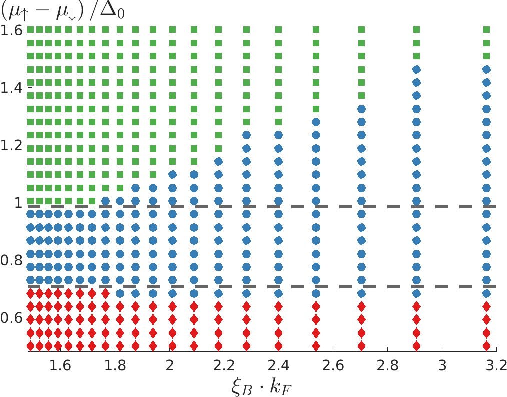
Figure 2: (Color online) The $T=0$ phase diagram of the bilayer fermions for $k_{F}d=1$ and $k_{F}a_{\text{eff}}=0.05$, as a function of the interaction range $\xi_{B}$ and the field $h$. The (red) diamonds, (blue) circles and (green) squares indicate the BCS, FF and normal phase, respectively. The horizontal dashed lines give the upper and lower critical fields for the FF phase for a short range interaction Shimahara (1994); Burkhardt and Rainer (1994).

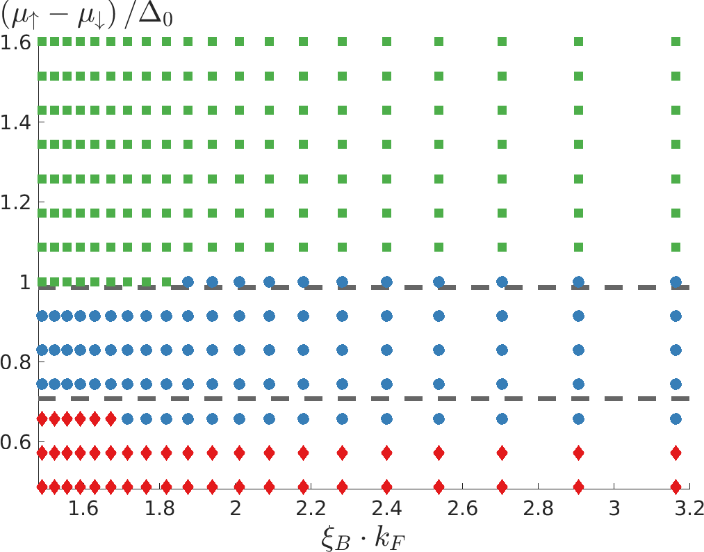
Figure 3: (Color online) The $T=0$ phase diagram of the bilayer fermions as a function of the interaction range $\xi_{B}$ and the field $h$ for zero layer distance and boson-fermion interaction strength $k_{F}a_{\text{eff}}=0.05$. The symbols and lines mean the same as in Fig. 2.

VI Berezinskii-Kosterlitz-Thouless Melting

Since the fermions are confined in 2D layers, phase fluctuations of the order parameter are significant and will eventually melt the superfluid through the Berezinskii-Kosterlitz-Thouless (BKT) mechanism at a critical temperature $T_{\text{BKT}}$. To describe this, we first calculate the superfluid stiffness, or equivalently the superfluid density, by imposing a linear phase twist on the order parameter and calculating the corresponding energy cost to second order in the twist. For a given vector $\mathbf{Q}$, the real space pairing becomes using Eq. (4)

$$\Delta(\mathbf{R},\mathbf{R})=\Delta\cdot e^{i(\mathbf{Q}+\delta\mathbf{q})\cdot{\mathbf{R}}},$$ (15)

where $\Delta=\sum_{\mathbf{k}}\Delta(\mathbf{k})/{\mathcal{V}}$ and $\delta\mathbf{q}\cdot{\mathbf{R}}=\delta\theta({\mathbf{R}})$ is the imposed spatially linear phase twist. From Eq. (15), it is clear that the direction of the phase twist relative to the COM of the Cooper pairs is important: When $\delta\mathbf{q}$ is parallel to $\mathbf{Q}$, the phase twist corresponds to adding/removing COM momentum to the Cooper pairs which compresses/expands the wavelength of the plane wave pairing field $\Delta(\mathbf{R},\mathbf{R})$; when $\delta\mathbf{q}$ is perpendicular to $\mathbf{Q}$, the phase twist corresponds to a small rotation of the COM momentum to the Cooper pairs which rotates the plane wave pairing field. These two effects are illustrated in Fig. 4(a).

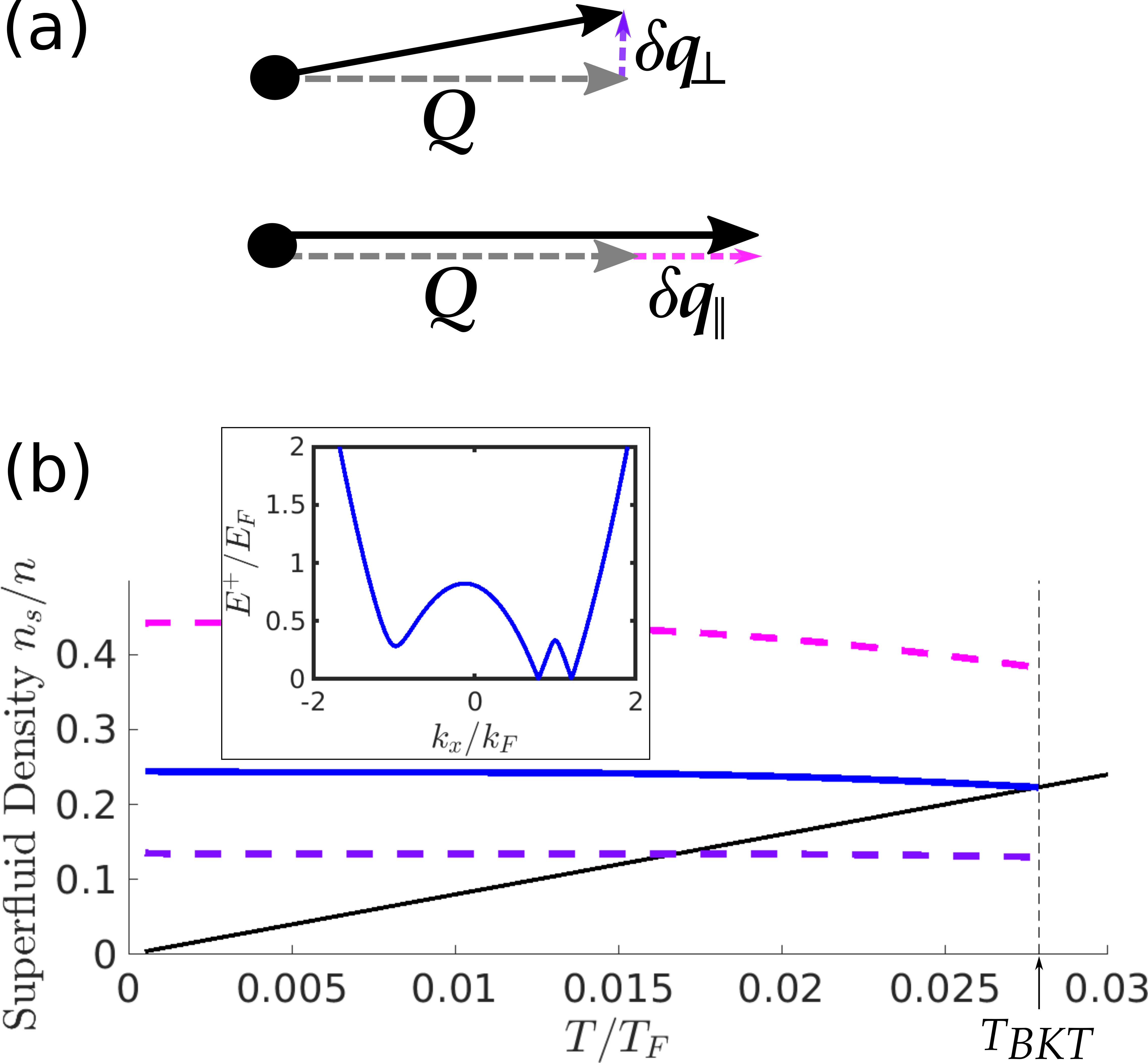
Figure 4: (Color online) (a) The two kinds of phase fluctuations with $\delta\mathbf{q}$ perpendicular and parallel to the COM momentum $\mathbf{Q}$ of the Cooper pairs give rise to a rotation and a compression/expansion of the plane wave pairing field respectively. (b) The corresponding superfluid densities $n_{s\parallel}$ (top dashed magenta line) and $n_{s\perp}$ (bottom dashed purple line). The solid blue line is to the effective superfluid density $n_{s}=\sqrt{n_{s\parallel}n_{s\perp}}$. The critical temperature $T_{\text{BKT}}$ is reached when $n_{s}$ crosses the thin solid black line as indicated by the vertical dashed line. The inset shows one branch of the quasiparticle spectrum along $k_{y}=0$ with the COM momentum $\mathbf{Q}$ along the $x$-axis for $T=0$. The gapless excitations leading to the reduction in the superfluid density are clearly visible.

The phase twist $\delta\theta({\mathbf{R}})$ gives a free energy cost $\delta F$ of the form

$$\delta F= \frac{1}{2}\int\!d^{2}{\mathbf{r}}[J_{\parallel}(\partial_{\parallel}\delta\theta)^{2}+J_{\perp}(\partial_{\perp}\delta\theta)^{2}]$$

$$= \frac{J}{2}\int\!d^{2}{\mathbf{r}}(\nabla\delta\theta)^{2},$$ (16)

where $\partial_{\parallel}$ and $\partial_{\perp}$ are spatial derivatives parallel or perpendicular to the COM momentum of the Cooper pairs, corresponding to $\delta\mathbf{q}\parallel\mathbf{Q}$ and $\delta\mathbf{q}\perp\mathbf{Q}$ respectively. The associated superfluid stiffness constants are $J_{\parallel}$ and $J_{\perp}$. In the second line of Eq. (16), we have rescaled the spatial coordinate perpendicular to $\mathbf{Q}$ by the factor $\sqrt{J_{\parallel}/J_{\perp}}$ to obtain an isotropic $XY$-model with the effective stiffness constant $J=\sqrt{J_{\parallel}J_{\perp}}$ Wu et al. (2016). Alternatively, defining the superfluid densities parallel and perpendicular to $\mathbf{Q}$ as $n_{s\perp}=4mJ_{\perp}$ and $n_{s\parallel}=4mJ_{\parallel}$, we can write the free energy cost as

$$\delta F=m\int\!d^{2}{\mathbf{r}}[n_{s\parallel}v_{s\parallel}^{2}+n_{s\perp}v_{s\perp}^{2}]/2.$$ (17)

Here $v_{s\parallel}=\partial_{\parallel}\delta\theta/2m$ is the superfluid velocity parallel to $\mathbf{Q}$ and likewise for $v_{s\perp}$. A long but straightforward calculation of the second order energy shift due to the phase twist gives

$$n_{s\parallel}=n-\frac{\beta}{m}\int\!d^{2}\check{k}[f_{\mathbf{k}}^{+}(1-f_{\mathbf{k}}^{+})+f_{\mathbf{k}}^{-}(1-f_{\mathbf{k}}^{-})]k_{\parallel}^{2}$$ (18)

for the superfluid density along $\mathbf{Q}$, where $k_{\parallel}=\mathbf{k}\cdot\mathbf{Q}/Q$. Here, $n$ is the total surface density of fermions coming from the two layers. An equivalent formula holds for $n_{s\perp}$. Equation (18) is the 2D version of the usual expression for the superfluid density allowing for the effects of the spatial anisotropy of the FF state Leggett (1975); Landau et al. (1980). We can now determine the critical temperature of the superfluid using the BKT condition

$$T_{\text{BKT}}=\frac{\pi}{2}J=\frac{\pi}{8m}n_{s}$$ (19)

where we have defined the effective superfluid density as $n_{s}=\sqrt{n_{s\parallel}n_{s\perp}}$.

In Fig. 4(b), we plot the superfluid densities as a function of $T$ for layer distance $k_{F}d=1$ and boson-fermion interaction strength $k_{F}a_{\text{eff}}=0.05$. We see that $n_{s\parallel}>n_{s\perp}$, reflecting that the energy cost related to compressing/expanding the COM momentum is higher than that related to rotating it as expected. Note that both superfluid densities are smaller than the total density $n$ even for $T\rightarrow 0$. This is due to the inherent presence of gapless quasiparticle states in the FF phase. These gapless excitations, which are shown in the inset of Fig. 4(b), reduce the superfluid density. We also plot the effective superfluid density $n_{s}=\sqrt{n_{s\parallel}n_{s\perp}}$ as well as the line $8mT/\pi$. It follows from Eq. (19) that the superfluid phase melts when $n_{s}$ crosses this line.

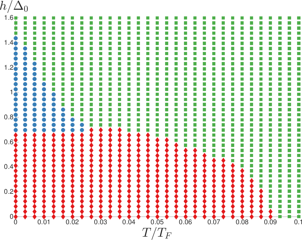
Figure 5: (Color online) The phase diagram as a function of temperature $T$ and field $h$ for layer distance $k_{F}d=1$, boson-fermion interaction strength $k_{F}a_{\text{eff}}=0.05$, and range $k_{F}\xi_{B}=3$. The symbols mean the same as in Figs. 2-3.

Having set up the theory for BKT melting, we can now analyse the BCS and FF phases at non-zero temperatures. In Fig. 5, we present an example of a phase diagram for $k_{F}d=1$ and $k_{F}a_{\text{eff}}=0.05$. We see that the critical temperature of the FF phase increases with decreasing field $h$. The highest critical temperature is obtained just above the lowest critical field $h_{c_{1}}$, where the FF, BCS, and normal phase meet in a tricritical point at $h_{c_{1}}\approx 0.7\Delta_{0}$ and $T\approx 0.025T_{F}$. This critical temperature is well below the theoretical maximum of $T_{F}/8$ obtained by setting $n_{s}=n$ in Eq. (19). The reason is that the gapless excitations in the FF phase decrease the superfluid density below $n$, as we discussed above in connection with Fig. 4. Indeed, we note that the value of the two components of the superfluid density in Fig. 4 at $T=T_{c}$ are almost unchanged from their value at $T\rightarrow 0$. This is a general result: While the flexibility of the bilayer system allows us to optimize the induced interaction to favour FF pairing, the gapless nature of this state prevents us from reaching critical temperatures close to $T_{F}/8$.

The critical temperature of the BCS phase is much higher as can be seen from Fig. 5. Due to its fully gapped spectrum, $T_{\text{BKT}}$ can in fact relatively easily be tuned to be close to maximum $T_{F}/8$ by varying the layer distance $d$, the interaction range $\xi_{B}$, even while keeping the boson-fermion interaction strength $a_{\text{eff}}$ weak.

VII Conclusion

We analysed a mixed-dimensional system consisting of two layers of identical fermions immersed in a BEC. This system was shown to support superfluid pairing due to an attractive induced interaction between the two layers mediated by the BEC. When the densities of the two layers are different, the resulting superfluid phase is inhomogeneous. Using a plane wave FF ansatz to describe this phase, we demonstrated that it is stabilised by the nonzero range of the induced interaction. Importantly, the FF phase can occupy much larger regions of the phase diagram as compared to the case of a short range interaction. The range of the induced interaction can be tuned by varying the BEC healing length, which makes the present system promising for realising FFLO physics experimentally. We furthermore analysed the melting of the superfluid phases due to phase fluctuations using BKT theory, and demonstrated that the normal, homogenous and inhomogeneous superfluid phases meet in a tricritical point in the phase diagram. The superfluid density of the FF phase was shown to be suppressed by intrinsic gapless excitations, and this leads to a significant reduction in the critical temperature compared to the homogeneous superfluid, which can be tuned to have a critical temperature close to the maximum $T_{F}/8$.