High-order rogue waves of a long wave-short wave model

Abstract

The long wave-short wave model describes the interaction between the long wave and the short wave. Exact higher-order rational solution expressed by determinants is calculated via the Hirota’s bilinear method and the KP hierarchy reduction. It is found that the fundamental rogue wave for the short wave can be classified into three different patterns: bright, intermediate and dark ones, whereas the rogue wave for the long wave is always bright type. The higher-order rogue waves correspond to the superposition of fundamental rogue waves. The modulation instability analysis show that the condition of the baseband modulation instability where an unstable continuous-wave background corresponds to perturbations with infinitesimally small frequencies, coincides with the condition for the existence of rogue-wave solutions.

PACS number(s): 05.45.Yv, 02.30.Ik, 02.30.Jr, 11.10.Lm

I Introduction

Rogue waves (RWs) or freak waves are rare phenomena that the large amplitudes appear from the background with the instability and unpredictability. Such extreme wave can be observed in various different contexts such as oceanography kharif2009rogue , hydrodynamic onorato2013rogue ; chabchoub2011rogue , Bose-Einstein condensate bludov2009matter , plasma bailung2011observation and nonlinear optic onorato2013rogue ; solli2007optical ; kibler2010peregrine . Mathematically, Peregrine soliton of the nonlinear Schrödinger (NLS) equation serves as a prototype of the RW, in which its structure is localized in temporal-spatial distribution plane and its maximum amplitude attains three times the background peregrine1983water . Since the higher-order RW was excited experimentally in wave tanks chabchoub2013observation ; chabchoub2012observation , a hierarchy of higher-order analytic RW solutions which indicate the superposition of elementary RW has been found in nonlinear integrable systems akhmediev2009rogue ; kedziora2012second ; dubard2010multi ; guo2012nonlinear ; ling2016multisoliton ; ohta2012general ; he2010generating ; wen2015generalized ; yang2015rogue ; chen2015rational . Moreover, in contrast to the scalar system, recent studies have shown that multicomponent coupled systems may allow some novel patterns of RW such as dark and four-petaled types guo2011roguewave ; ling2012highorder ; baronio2012solutions ; zhao2013roguewave ; baronio2013solutions ; zhao2016high ; ling2016darboux ; chen2014dark ; chow2013rogue ; mu2015dynamics ; wang2015roguewave ; zhang2017solitons ; wen2015modulational .

Modulation instability (MI) refers to the basic process that the growth of perturbations emerges on an unstable continuous wave background zakharov2009modulation . In the explanations of the generation mechanism for the RW, MI has been found to be closely linked with the RW excitation in nonlinear dispersive systems baronio2014vector ; baronio2015baseband ; zhao2016quantitative ; biondini2016universal . It has been shown that RW modeled as rational solutions only exist in the subset of parameters where MI is present if and only if the unstable sideband spectrum also contains continuous wave or zero-frequency perturbations as a limiting case baronio2014vector ; baronio2015baseband .

To discover how waves with different length scales (frequencies) interact and affect each other, Benny established the general theory for the interaction between the long wave (LW) and the short wave (SW) benney1977general . Particularly, under the certain resonance condition, namely, the phase velocity of the LW is equal to the group velocity of the SW, energy exchange can be anticipated and the resonance interaction occurs benney1977general . Such resonance process may appear in a variety of physical settings such as capillary-gravity waves, internal-surface waves, short and long gravity waves on fluids of finite depth and the breakdown of laminar flow benney1977general ; newell1978long ; newell1979general .

The aim of the present work is investigate RWs for a coupled system with the LW interacting the SW via the KP hierarchy reduction, and discuses the mechanism for the RW excitation through the MI anylsis. The outline of the present paper is as follows. In Sec. II, general analytical higher-order rational solutions in terms of determinants with algebraic elements are derived via the Hirota’s bilinear method and the KP hierarchy reduction. In Sec. III, local structures of RWs are analyzed and show that the SW possesses bright, intermediate and dark patterns, whereas the LW always exhibits bright state in the fundamental RW. The higher-order RWs indicate the superposition of fundamental ones and interaction behaviors among different types of the RW can’t occur in such pure higher-order rational solutions. In Sec. IV, MI analysis is carried out to find that the condition of baseband MI coincides with the condition for the existence of rogue-wave solutions. Numerical simulations are also provided to show RW excitation in the regime of baseband MI. A discussion is given and results are summarized in Sec. V.

II High-order rational solution in the determinant form

Based on the Benney theory for the interaction between the SW and the LW benney1977general , an integrable long wave-short wave (LWSW) model newell1978long ; newell1979general is proposed

$${\rm i}S_{t}+S_{xx}-2{\rm i}S_{x}L=0,$$ (1)

$$L_{t}=-2\sigma(|S|^{2})_{x},$$ (2)

where $S=S(x,t)$ represents the envelope of the short wave and $L=L(x,t)$ denotes the amplitude of the long wave. The complete integrability of the LWSW model (1)-(2) was tested by Painlevé analysis chowdhury1986complete . Ling et al. constructed its Darboux transformation and found a closed multi-soliton solution formula ling2011long ; huang2013darboux . A class of cusp solution for the LWSW model (1)-(2) was derived by using the dressing method zhu2015cusp . Geng et al. provided this coupled system’s algebro-geometric constructions and their explicit theta function representations geng2017algebro .

By the dependent variable transformation

$$S=\rho{\rm e}^{{\rm i}[\alpha x-\alpha^{2}t]}\frac{g}{f^{*}},\ \ L={\rm i}\frac{\partial}{\partial x}\ln\frac{f^{*}}{f},$$ (3)

where $\rho$ and $\alpha$ are real parameters, the LWSW model (1)-(2) can be cast into the bilinear form

$$({\rm i}D_{t}+2{\rm i}\alpha D_{x}+D^{2}_{x})g\cdot f=0,$$ (4)

$${\rm i}D_{t}f\cdot f^{*}=D^{2}_{x}f\cdot f^{*},$$ (5)

$${\rm i}D_{t}f\cdot f^{*}=-2\sigma\rho^{2}(|f|^{2}-|g|^{2}).$$ (6)

where $f$ and $g$ are complex variables, $*$ denotes the complex conjugation and $D$ is Hirota’s bilinear differential operator. Then we first present the general rational solutions of the LWSW model (1)-(2) in the following theorem. The proof of this theorem is given in the Appendix.

Theorem 2.1 The LWSW equations (1)-(2) have the rational solutions (3) with the tau functions $f$ and $g$ given by $N\times N$ determinants

$$f=\tau_{-1,0},\ \ g=\tau_{-1,1}$$ (7)

where

$$\tau_{n,k}=\det_{1\leq i,j\leq N}\left(m^{(N-i,N-j,n,k)}_{2i-1,2j-1}\right)=\begin{vmatrix}m_{11}^{(N-1,N-1,n,k)}&m_{13}^{(N-1,N-2,n,k)}&\cdots&m_{1,2N-1}^{(N-1,0,n,k)}\\ m_{31}^{(N-2,N-1,n,k)}&m_{33}^{(N-2,N-2,n,k)}&\cdots&m_{3,2N-1}^{(N-2,0,n,k)}\\ \vdots&\vdots&&\vdots\\ m_{2N-1,1}^{(0,N-1,n,k)}&m_{2N-1,3}^{(0,N-2,n,k)}&\cdots&m_{2N-1,2N-1}^{(0,0,n,k)}\end{vmatrix},$$ (8)

and the matrix elements are defined by

$$m^{(\nu,\mu,n,k)}_{i,j}=\left.\sum_{l=0}^{i}\sum_{s=0}^{j}\frac{a_{l}^{(\nu)}}{(i-l)!}\frac{a_{s}^{(\mu)*}}{(j-s)!}[(p-{\rm i}\alpha)\partial_{p}]^{i-l}[(q+{\rm i}\alpha)\partial_{q}]^{j-s}m^{(n,k)}\right|_{p=\zeta,q=\zeta^{*}},$$ (9)

with

$$m^{(n,k)}=\frac{{\rm i}p}{p+q}\left(-\frac{p}{q}\right)^{n}\left(-\frac{p-{\rm i}\alpha}{q+{\rm i}\alpha}\right)^{k}e^{(p+q)x-(p^{2}-q^{2}){\rm i}t},$$ (10)

$$a^{(\nu+1)}_{l}=\sum^{l}_{j=0}\frac{2^{j+2}(p-{\rm i}\alpha)^{2}+(-1)^{j}\frac{2{\rm i}\sigma\alpha\rho^{2}}{p-{\rm i}\alpha}+2{\rm i}\alpha(p-{\rm i}\alpha)}{(j+2)!}a^{(\nu)}_{l-j},\ \ \nu=0,1,2,\cdots,$$ (11)

and $\zeta$ need to satisfies the relation

$$2\zeta-\frac{2\sigma{\rm i}\alpha\rho^{2}}{(\zeta-{\rm i}\alpha)^{2}}=0.$$ (12)

III Dynamics of rogue wave solutions

III.1 Fundamental rogue wave

According to Theorem 2.1, in order to obtain the first-order rogue wave, we need to take $N=1$ in Eqs.(7)-(12). For simplicity, we set $a^{(0)}_{0}=b^{(0)}_{0}=1$ and $a^{(0)}_{1}=b^{(0)}_{1}=0$, then the functions $f$ and $g$ take the form

$$f=\frac{1}{\zeta^{3}_{1}}e^{2\zeta_{1}(x-2\zeta_{2}t)}F,$$ (13)

$$g=\frac{1}{\zeta^{3}_{1}}e^{2\zeta_{1}(x-2\zeta_{2}t)}\left[-\frac{\zeta_{1}+{\rm i}(\zeta_{2}-\alpha)}{\zeta_{1}-{\rm i}(\zeta_{2}-\alpha)}\right]\left[F+l_{1}-{\rm i}l_{2}\right],$$ (14)

with

$$F=-\Delta\left[\frac{\zeta_{2}}{2}\theta^{2}_{1}+2\zeta_{2}\theta^{2}_{2}+\theta_{0}+{\rm i}\frac{\zeta_{1}}{2}(h^{2}_{1}+h^{2}_{2})\right],$$ (15)

and $\Delta=\zeta^{2}_{1}+(\zeta_{2}-\alpha)^{2}$, $\theta_{1}=\zeta_{1}x-2\zeta_{1}\zeta_{2}t-\frac{1}{2}$, $\theta_{2}=\zeta^{2}_{1}t-\frac{\zeta_{1}}{4\zeta_{2}}$, $\theta_{0}=\frac{\zeta^{2}_{2}-\zeta^{2}_{1}}{4\zeta_{2}}$, $h_{1}=\zeta_{1}(x-2\zeta_{2}t)$, $h_{2}=2\zeta^{2}_{1}t$, $l_{1}=\zeta^{2}_{1}\left(\zeta_{1}l_{0}+\frac{\zeta_{2}}{2}\right)$, $l_{2}=\zeta_{1}\zeta_{2}\left(\zeta_{1}l_{0}+\frac{\zeta_{2}-\alpha}{2}\right)$, and $l_{0}=(\alpha-\zeta_{2})x-2(\zeta^{2}_{1}-\zeta^{2}_{2}+\alpha\zeta_{2})t$.

Therefore, the fundamental rogue wave solution for the LWSW model (1)-(2) reads

$$S=\rho{\rm e}^{{\rm i}[\alpha x-\alpha^{2}t]}\left[-\frac{\zeta_{1}+{\rm i}(\zeta_{2}-\alpha)}{\zeta_{1}-{\rm i}(\zeta_{2}-\alpha)}\right]\left\{1-\frac{\zeta^{2}_{1}\left(\zeta_{1}l_{0}+\frac{\zeta_{2}}{2}\right)-{\rm i}\left[\zeta_{1}\zeta_{2}\left(\zeta_{1}l_{0}+\frac{\zeta_{2}-\alpha}{2}\right)-\Delta\zeta_{1}(h^{2}_{1}+h^{2}_{2})\right]}{\Delta\left[\frac{\zeta_{2}}{2}\theta^{2}_{1}+2\zeta_{2}\theta^{2}_{2}+\theta_{0}-{\rm i}\frac{\zeta_{1}}{2}(h^{2}_{1}+h^{2}_{2})\right]}\right\},$$ (16)

$$L=-4\frac{\zeta^{2}_{1}[\zeta_{2}\theta_{1}(h^{2}_{1}+h^{2}_{2}-h_{1}\theta_{1})-2h_{1}(\theta_{0}+2\zeta_{2}\theta^{2}_{2})]}{\left(\zeta_{2}\theta^{2}_{1}+4\zeta_{2}\theta^{2}_{2}+2\theta_{0}\right)^{2}+\zeta^{2}_{1}(h^{2}_{1}+h^{2}_{2})^{2}}.$$ (17)

Furthermore, the modular square of the SW component $|S|^{2}$ possesses extrema (turning points where the first derivatives vanish)

$$(x_{1},t_{1})=\left(\frac{\zeta^{2}_{2}}{\zeta_{1}(\zeta^{2}_{1}+\zeta^{2}_{2})},\frac{1}{4}\frac{\zeta_{2}}{\zeta_{1}(\zeta^{2}_{1}+\zeta^{2}_{2})}\right),$$ (18)

$$(x_{2},t_{2})=\left(\frac{\zeta_{2}(\alpha^{2}-\zeta^{2}_{1}-\zeta^{2}_{2})}{2\zeta_{1}\Delta_{3}}-\frac{2\Delta_{5}\mu_{1}}{\Delta_{1}\Delta_{3}\zeta^{2}_{1}},\frac{\mu_{1}}{\Delta_{1}\zeta^{2}_{1}}\right),$$ (19)

$$(x_{3},t_{3})=\left(-\frac{\zeta_{2}(\alpha^{2}-\zeta^{2}_{1}-\zeta^{2}_{2})}{2\zeta_{1}\Delta_{6}}+\frac{2\Delta_{7}\mu_{2}}{\Delta_{1}\Delta_{6}\zeta_{1}},\frac{\mu_{2}}{\Delta_{1}\zeta^{2}_{1}}\right),$$ (20)

with $\mu_{1}=\frac{\zeta_{1}\zeta_{2}\Delta_{1}}{4(\zeta^{2}_{1}+\zeta^{2}_{2})}\pm\frac{\sqrt{-\zeta_{2}\Delta_{2}\Delta^{2}_{3}\Delta_{4}}}{4(\zeta^{2}_{1}+\zeta^{2}_{2})\Delta_{2}}$, $\mu_{2}=\frac{\zeta_{2}\Delta_{1}}{4(\zeta^{2}_{1}+\zeta^{2}_{2})}\pm\frac{\sqrt{\zeta_{2}\Delta^{2}_{6}\Delta_{8}\Delta_{9}}}{4(\zeta^{2}_{1}+\zeta^{2}_{2})\Delta_{9}}$, $\Delta_{1}=\zeta^{2}_{1}+(\zeta_{2}-\alpha)^{2}$, $\Delta_{2}=\zeta^{2}_{1}+(\zeta_{2}+\alpha)^{2}$, $\Delta_{3}=\alpha(2\zeta^{2}_{1}+\alpha\zeta_{2})-\zeta_{2}(\zeta^{2}_{1}+\zeta^{2}_{2})$, $\Delta_{4}=\zeta_{2}(\zeta^{2}_{1}+\zeta^{2}_{2})-2(2\zeta^{2}_{1}+\zeta^{2}_{2})\alpha+\zeta_{2}\alpha^{2}$, $\Delta_{5}=(\zeta^{2}_{2}-\zeta^{2}_{1})(\zeta^{2}_{1}+\zeta^{2}_{2}-\alpha^{2})-4\alpha\zeta_{2}\zeta^{2}_{1}$, $\Delta_{6}=3\zeta_{2}(\zeta^{2}_{1}+\zeta^{2}_{2})-2\alpha(\zeta^{2}_{1}+2\zeta^{2}_{2})+\zeta_{2}\alpha^{2}$, $\Delta_{7}=-(\zeta^{2}_{1}+\zeta^{2}_{2})(\zeta^{2}_{1}-5\zeta^{2}_{2})-4\zeta_{2}(\zeta^{2}_{1}+2\zeta^{2}_{2})\alpha+(\zeta^{2}_{1}+3\zeta^{2}_{2})\alpha^{2}$, $\Delta_{8}=3\zeta_{2}(\zeta^{2}_{1}+\zeta^{2}_{2})-2(2\zeta^{2}_{1}+3\zeta^{2}_{2})\alpha+3\zeta_{2}\alpha^{2}$ and $\Delta_{9}=(\zeta^{2}_{1}+\zeta^{2}_{2})(\zeta^{2}_{1}+4\zeta^{2}_{2})-2\zeta_{2}(3\zeta^{2}_{1}+4\zeta^{2}_{2})\alpha+(\zeta^{2}_{1}+4\zeta^{2}_{2})\alpha^{2}$.

Note that $(x_{2},t_{2})$ are also two characteristic points, at which the values of the amplitude are zero. Through the local analysis, the fundamental rogue wave for short wave can be classified into three patterns. Without loss of generality, we take $\rho=1$, then there are two different cases:

In the case of $\sigma=1$: (a) Dark state ($|\alpha|\leq\frac{\sqrt{-378+66\sqrt{33}}}{12}$): two local maxima at $(x_{3},t_{3})$ and one local minimum at $(x_{1},t_{1})$. Especially, when $|\alpha|=\frac{\sqrt{-378+66\sqrt{33}}}{12}$, the local minimum at the characteristic point $(x_{1},t_{1})=(x_{2},t_{2})$. (b) Intermediate state $(\frac{\sqrt{-378+66\sqrt{33}}}{12}<|\alpha|<\frac{\sqrt{-18+6\sqrt{33}}}{4})$: two local maxima at $(x_{3},t_{3})$ and two local minima at the characteristic point $(x_{2},t_{2})$. (c) Bright state ($\frac{\sqrt{-18+6\sqrt{33}}}{4})\leq|\alpha|$ ): one local maximum at $(x_{1},t_{1})$ and two local minima at $(x_{2},t_{2})$. When the sign takes ”=”, the local maximum at $(x_{1},t_{1})=(x_{3},t_{3})$.

In the case of $\sigma=-1$ ($|\alpha|<\frac{3}{2}\sqrt{3}$ and $|\alpha|\neq\frac{\sqrt{2}}{2}$): (a) Dark state ($\frac{\sqrt{378+66\sqrt{33}}}{12}\leq|\alpha|<\frac{3}{2}\sqrt{3}$): two local maxima at $(x_{3},t_{3})$ and one local minimum at $(x_{1},t_{1})$. Especially, when $|\alpha|=\frac{\sqrt{378+66\sqrt{33}}}{12}$, the local minimum at the characteristic point $(x_{1},t_{1})=(x_{2},t_{2})$. (b) Intermediate state $(\frac{\sqrt{18+6\sqrt{33}}}{4}<|\alpha|<\frac{\sqrt{378+66\sqrt{33}}}{12})$: two local maxima at $(x_{3},t_{3})$ and two local minima at the characteristic point $(x_{2},t_{2})$. (c) Bright state ( $|\alpha|\leq\frac{\sqrt{18+6\sqrt{33}}}{4}$ ): (i) $\frac{\sqrt{2}}{2}<|\alpha|\leq\frac{\sqrt{18+6\sqrt{33}}}{4}$: one local maximum at $(x_{1},t_{1})$ and two local minima at $(x_{2},t_{2})$; (ii) $|\alpha|<\frac{\sqrt{2}}{2}$: one local maximum at $(x_{1},t_{1})$ and two local minima at $(x_{3},t_{3})$. When the sign takes ”=”, the local maximum at $(x_{1},t_{1})=(x_{3},t_{3})$.

For the LW component $L$, it possesses extrema $(x_{1},t_{1})$ and

$$(x_{4},t_{4})=\left(\frac{2(\zeta^{2}_{1}+3\zeta^{2}_{2})}{\zeta_{1}}\mu_{3}-\frac{1}{2\zeta_{1}},\frac{\zeta_{2}}{\zeta_{1}}\mu_{3}\right),$$ (21)

with $\mu_{3}=\frac{1}{4(\zeta^{2}_{1}+\zeta^{2}_{2})}\pm\frac{\sqrt{3}}{4}\frac{\sqrt{\zeta^{2}_{2}(\zeta^{2}_{1}+4\zeta^{2}_{2})}}{(\zeta^{2}_{1}+\zeta^{2}_{2})(\zeta^{2}_{1}+4\zeta^{2}_{2})}$. The further local analysis shows that in both cases $\sigma=\pm 1$, the rogue wave for the LW component only exhibits bright state with one local maximum at $(x_{1},t_{1})$ and two local minima at $(x_{4},t_{4})$.

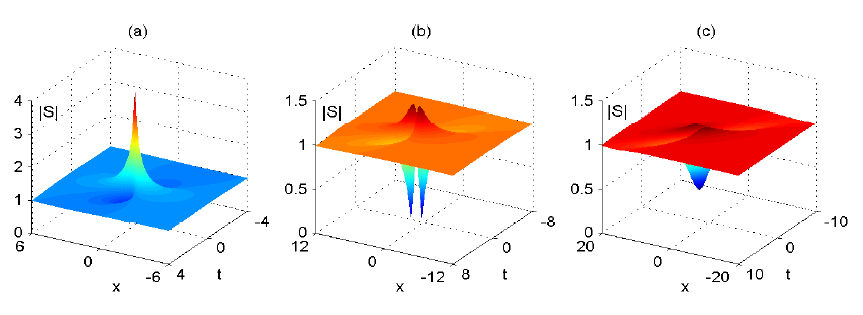
Figure 1: First-order rogue wave for the SW in the LWSW model (1)-(2) with the parameters $\rho=-\sigma=1$ and (a) bright state $\alpha=1.5$; (b) intermediate state $\alpha=2.1$ and (c) dark state $\alpha=2.3$.

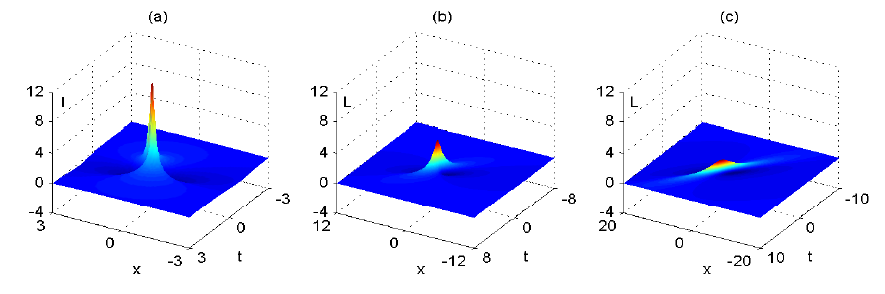
Figure 2: First-order rogue wave for the LW in the LWSW model (1)-(2) with the parameters $\rho=-\sigma=1$ and (a) $\alpha=1.5$; (b) $\alpha=2.1$ and (c) $\alpha=2.3$, respectively.

As illustrated in Fig. 1, three types of RW exhibit different local structures for the SW when the parameter $\alpha$ takes the value in its corresponding regimes. It implies that RW’s pattern for the SW component is dependent on $\alpha$, which decides the number, the position, the height and the type of extrema. Fig 2 displays the RW states of the LW, three cases correspond to the same parameters’ choices as shown in Fig.1. It is easy to see that as $\alpha$ increases, the local structure of the LW always features the bright RW only the central amplitude decreases.

For the LWSW model (1)-(2), it can be viewed as a coupling extension of the derivative NLS (DNLS) equation, exactly the Chen-Lee-Liu (CLL) equation. We recall that the DNLS equation only supports the RW of bright type with two zero-amplitude points. Here, due to the coupling component $L$ which leads to complex interplay between the dispersion and the nonlinearity, dark and intermediate RWs appear for the SW component. From the local analysis, one can know that two kinds of the bright RW emerge under the different parameters’ conditions. Specifically, the normal bright RW with two characteristic points can be realized in the regions $|\alpha|\geq\frac{\sqrt{-18+6\sqrt{33}}}{4}$ ($\sigma=1$) and $\frac{\sqrt{2}}{2}<|\alpha|\leq\frac{\sqrt{18+6\sqrt{33}}}{4}$ ($\sigma=-1$). The another case ($|\alpha|<\frac{\sqrt{2}}{2}$ for $\sigma=-1$) corresponds to a sepcial bright RW which also possesses one maximum and two minima amplitudes but two local minima are not characteristic points. The intermediate RW is always characterized by two local maxima and two local minima at zero-amplitude points. For the dark RW, its amplitude possesses two local maxima and one local minimum which usually can’t attain zero. But at the critical cases between the dark RW and the intermediate one in which $\alpha$ takes $|\alpha|=\frac{\sqrt{-\sigma 378+66\sqrt{33}}}{12}$, the local minimum occurs at zero-amplitude points. In this situation, the dark RW reduces to a special one which can be referred to a black RW.

III.2 High-order rogue wave

The second-order rogue wave solution is obtained from Eqs.(7)–(10) with $N=2$. In this case, setting $a^{(0)}_{0}=b^{(0)}_{0}=1$, $a^{(0)}_{1}=b^{(0)}_{1}=0$, $a^{(0)}_{2}=b^{(0)}_{2}=0$, we obtain the functions $f$ and $g$ as follows

$$f=\begin{vmatrix}m_{11}^{(1,1,-1,0)}&m_{13}^{(1,0,-1,0)}\\ m_{31}^{(0,1,-1,0)}&m_{33}^{(0,0,-1,0)}\end{vmatrix},\ \ g=\begin{vmatrix}m_{11}^{(1,1,-1,1)}&m_{13}^{(1,0,-1,1)}\\ m_{31}^{(0,1,-1,1)}&m_{33}^{(0,0,-1,1)}\end{vmatrix}\,,$$ (22)

where the elements are determined by

$$m_{11}^{(1,1,n,k)}=A^{(1)}_{1}B^{(1)}_{1}\left.m^{(n,k)}\right|_{p=\zeta,q=\zeta^{*}},\ \ m_{13}^{(1,0,n,k)}=A^{(1)}_{1}B^{(0)}_{3}\left.m^{(n,k)}\right|_{p=\zeta,q=\zeta^{*}},$$

$$m_{31}^{(0,1,n,k)}=A^{(0)}_{3}B^{(1)}_{1}\left.m^{(n,k)}\right|_{p=\zeta,q=\zeta^{*}},\ \ m_{33}^{(0,0,n,k)}=A^{(0)}_{3}B^{(0)}_{3}\left.m^{(n,k)}\right|_{p=\zeta,q=\zeta^{*}},$$

and the differential operators $A^{(1)}_{1}=a^{(1)}_{0}(p-{\rm i}\alpha)\partial_{p}+a^{(1)}_{1}$, $B^{(1)}_{1}=a^{(1)*}_{0}(q+{\rm i}\alpha)\partial_{q}+a^{(1)*}_{1}$, $A^{(0)}_{3}=\frac{1}{6}[(p-{\rm i}\alpha)\partial_{p}]^{3}+a^{(0)}_{3}$, $B^{(0)}_{3}=\frac{1}{6}[(q+{\rm i}\alpha)\partial_{q}]^{3}+a^{(0)*}_{3}$ with $a^{(1)}_{0}=2(p-{\rm i}\alpha)^{2}+\frac{{\rm i}\sigma\alpha\rho^{2}}{p-{\rm i}\alpha}+{\rm i}\alpha(p-{\rm i}\alpha)$ and $a^{(1)}_{1}=\frac{1}{3}\left[4(p-{\rm i}\alpha)^{2}-\frac{{\rm i}\sigma\alpha\rho^{2}}{p-{\rm i}\alpha}+{\rm i}\alpha(p-{\rm i}\alpha)\right]$.

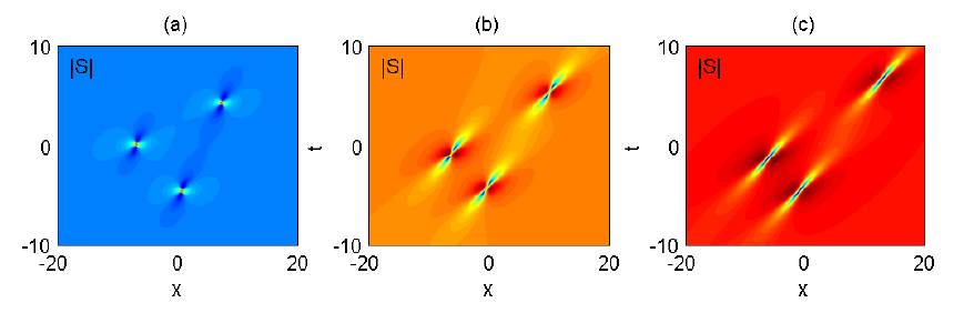
Figure 3: Second-order rogue wave for the SW in the LWSW model (1)-(2) with the parameters $\rho=-\sigma=1$, $a_{0}^{(0)}=1,a^{(0)}_{1}=a^{(0)}_{2}=0,a^{(0)}_{3}=350$ and (a) bright state $\alpha=1.5$; (b) intermediate state $\alpha=2.1$ and (c) dark state $\alpha=2.3$.

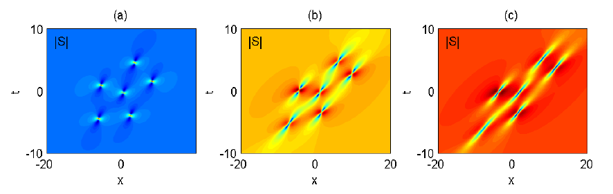
Figure 4: Third-order rogue wave for the SW in the LWSW model (1)-(2) with the parameters $\rho=-\sigma=1$, $a_{0}^{(0)}=1,a^{(0)}_{1}=a^{(0)}_{2}=a^{(0)}_{3}=a^{(0)}_{4}=0,a^{(0)}_{5}=2000$ and (a) bright state $\alpha=1.5$; (b) intermediate state $\alpha=2.1$ and (c) dark state $\alpha=2.3$.

Since the LW always features a bright RW, we only present the configuration of the SW to illustrate higher RWs. Three second-order RWs for the SW are displayed in Fig.3, each one takes the same value of the parameter $\alpha$ as one shown in Fig.1. One can observe that second-order RWs manifest the superposition of three fundamental ones and they obey the triangle arrays. Owing to the same parameters $\alpha$ as the first-order cases respectively, three second-order RWs exhibit pure dark, intermediate and bright RW’s combinations individually.

For third and higher-order RWs, which describe the superposition of more fundamental RWs, one need to take larger $N$ in (7)-(12). The expressions are too complicated to be written here. Fig.4 shows the third-order RW for $N=3$ graphically, in which three plots still take the same parameter $\alpha$ as Figs.1 and 3. It can be seen that third-order RWs exhibit the superposition of six fundamental ones and they constitute a shape of pentagon. Besides, each combination only contains one type of elementary RW purely in three cases, which coincides with ones of first and second-order cases. This fact suggests that only three types of RW happens whether the RW is fundamental or higher-order one for the SW and the RW’s pattern completely depends on the parameter $\alpha$. For instance, when $\sigma=1$, three types of RW (fundamental one and higher-order superposition) strictly takes place at at three intervals of $\alpha$, i.e. $|\alpha|\leq\frac{\sqrt{-378+66\sqrt{33}}}{12}$ for dark state, $\frac{\sqrt{-378+66\sqrt{33}}}{12}<|\alpha|<\frac{\sqrt{-18+6\sqrt{33}}}{4}$ for intermediate state and $\frac{\sqrt{-18+6\sqrt{33}}}{4})\leq|\alpha|$ for bright state. That is to say, the construction of higher-order RW solutions here don’t allow the mixed superposition among different types of fundamental RWs.

IV Modulation Instability

Next we investigate the linear stability analysis of the LWSW model by considering small perturbations of the form $S=[a+S_{1}]e^{{\rm i}[\omega x-(\omega^{2}-2b\omega)t]}$ and $L=b+L_{1}$. The substitution yields a group of linearized partial differential equations. Recalling that $L$ is real, we can assume the perturbations are space periodic with the fixed frequency $\Omega$, i.e., $S_{1}=s_{1}(t)e^{{\rm i}\Omega x}+s_{2}(t)e^{-{\rm i}\Omega x}$ and $L_{1}=l(t)e^{{\rm i}\Omega x}+l^{*}(t)e^{-{\rm i}\Omega x}$, which leads the above linearized partial differential equations into a group of linear ordinary differential equations $s^{\prime}={\rm i}Ms$ with $s=[s_{1},s^{*}_{2},l]^{T}$ and

$$M=\left[\begin{matrix}-\Omega^{2}+2b\Omega-2\omega\Omega&0&2a\omega\\ 0&\Omega^{2}+2b\Omega-2\omega\Omega&-2a\omega\\ -2a\sigma\Omega&-2a\sigma\Omega&0\end{matrix}\right].$$ (23)

This set of differential equations with the real frequency $\Omega$ suggests that the functions $s_{1}(t)$, $s_{2}(t)$ and $l(t)$ are the linear combinations of exponentials $\exp({\rm i}\lambda_{j}t)$ where $\lambda_{j}$, $j=1,2,3$ represent three eigenvalues of the matrix $M$. Such eigenvalues are given by the roots of the characteristic polynomial $P(\lambda)$ of the matrix $M$,

$$P(\lambda)=\lambda^{3}+P_{2}\lambda^{2}+P_{1}\lambda+P_{0},$$ (24)

with $P_{2}=4(\omega-b)\Omega$, $P_{1}=[4(b-\omega)^{2}-\Omega^{2}]\Omega^{2}$ and $P_{0}=-8\sigma\omega a^{2}\Omega^{3}$.

It is known that when an eigenvalue has a negative imaginary part, MI will occur with the exponential growing perturbation. From the matrix $M$, one can find each entry is real, so the corresponding eigenvalues are either real root, or a pair of complex-conjugate roots. More specifically, we calculate the discriminant of the characteristic polynomial $P(\lambda)$ as

$$\Delta=4\Omega^{6}\left\{3\Omega^{6}-24(b-\omega)^{2}\Omega^{4}-48(b-\omega)[9\sigma\omega a^{2}-(b-\omega)^{3}]\Omega^{2}-48\sigma\omega a^{2}[27\sigma\omega a^{2}-4(b-\omega)^{3}]\right\}.$$ (25)

Then, $\Delta>0$ results in real roots for the polynomial $P(\lambda)$, which implies that no MI appears, whereas $\Delta<0$ yields two complex conjugate roots, which suggests that MI exists. The marginal stability curves corresponds to the discriminant $\Delta=0$. Without loss of generality, by taking $a=1$ and $b=0$, MI gain spectrums of the LWSW model (1)-(2) are displayed for two kinds of nonlinearity $\sigma=1$ and $\sigma=-1$ in Fig.5 respectively.

As analyzed in baronio2014vector ; baronio2015baseband , baseband MI defined as the condition where an unstable continuous-wave background corresponds to perturbations infinitesimally small frequencies, is responsible for RW excitation, whereas passband MI which means the perturbation undergoes gain in a spectral region not including zero frequency as a limiting case, doesn’t support the RW. Thus the limit situation where $\Omega\rightarrow 0$ decides the occurrence of baseband MI. In this case, the discriminant of the polynomial $P(\lambda)$ degenerates to $\Delta=-48\sigma\omega(4\omega^{3}+27\sigma\omega)$, which gives rise to two cases: (1) $\sigma=1$, no MI and (2) $\sigma=-1$, MI condition $|\omega|<\frac{3}{2}\sqrt{3}$. The coincidence is that the baseband MI condition is exactly one for the existence of rogue-wave solutions.

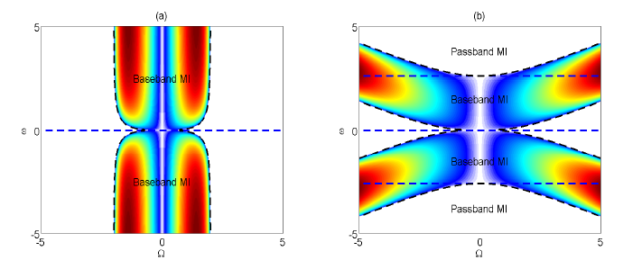
Figure 5: MI for the LWSW model (1)-(2) on the $(\Omega,\omega)$ plane, calculated with the parameters $a=1$, $b=0$, (a):$\sigma=1$ and (b):$\sigma=-1$. Dark dashed curves represent the analytical marginal stability condition $\Delta=0$.

V Conclusion

The long wave-short wave model describes the interaction between the long wave and the short wave. Exact higher-order rational solution expressed by determinants is calculated via the Hirota’s bilinear method and the KP hierarchy reduction. It is found that the fundamental rogue wave for the SW can be classified into three different patterns: bright, intermediate and dark ones, whereas the rogue wave for the LW is always bright type. The higher-order rogue waves correspond to the superposition of fundamental rogue waves. The modulation instability analysis show that the condition of the baseband modulation instability where an unstable continuous-wave background corresponds to perturbations with infinitesimally small frequencies, coincides with the condition for the existence of rogue-wave solutions.

Appendix

In this Appendix we will prove Theorem 2.1 in Sec. II via the KP hierarchy reduction. First we present the following lemma.

Lemma 1 The bilinear equations in the extended KP hierarchy

$$(D_{x_{2}}-2aD_{x_{1}}-D^{2}_{x_{1}})\tau_{n,k+1}\cdot\tau_{n,k}=0,$$ (A1)

$$(D_{x_{2}}+D^{2}_{x_{1}})\tau_{n,k}\cdot\tau_{n+1,k}=0,$$ (A2)

$$(aD_{t_{a}}+1)\tau_{n,k}\cdot\tau_{n+1,k}=\tau_{n,k+1}\tau_{n+1,k-1},$$ (A3)

where $a$ is a complex constant, $n$ and $k$ are integers, have the following solution

$$\tau_{n,k}=\tilde{m}^{(n,k)}=\frac{{\rm i}p}{p+q}\left(-\frac{p}{q}\right)^{n}\left(-\frac{p-a}{q+a}\right)^{k}{\rm e}^{\tilde{\xi}+\tilde{\eta}},$$ (A4)

with

$$\tilde{\xi}=\frac{1}{p-a}t_{a}+px_{1}+p^{2}x_{2},\ \ \tilde{\eta}=\frac{1}{q+a}t_{a}+qx_{1}-q^{2}x_{2},$$

where $p$, $q$ and $a$ are complex parameters.

In order to derive the rational soluiton, we introduce the differential operators $A_{k}^{(\nu)}$ and $B_{l}^{(\mu)}$ with respect to $p$ and $q$ respectively

$$A_{n}^{(\nu)}=\sum_{k=0}^{n}a_{k}^{(\nu)}\frac{[(p-a)\partial_{p}]^{n-k}}{(n-k)!},\quad n\geq 0,$$ (A5)

$$B_{n}^{(\nu)}=\sum_{k=0}^{n}b_{k}^{(\nu)}\frac{[(q+a)\partial_{q}]^{n-k}}{(n-k)!},\quad n\geq 0,$$ (A6)

where $a_{k}^{(\nu)}$ and $b_{k}^{(\nu)}$ are constants satisfying the iterated relations

$$a^{(\nu+1)}_{k}=\sum^{k}_{j=0}\frac{2^{j+2}(p-a)^{2}+(-1)^{j}\frac{\lambda a}{p-a}+2a(p-a)}{(j+2)!}a^{(\nu)}_{k-j},\ \ \nu=0,1,2,\cdots,$$ (A7)

$$b^{(\nu+1)}_{k}=\sum^{k}_{j=0}\frac{2^{j+2}(q+a)^{2}-(-1)^{j}\frac{\lambda a}{q+a}-2a(q+a)}{(j+2)!}b^{(\nu)}_{k-j},\ \ \nu=0,1,2,\cdots\,.$$ (A8)

Based on the Leibniz rule, one has

$$[(p-a)\partial_{p}]^{m}\left(p^{2}+\frac{\lambda a}{p-a}\right) = \sum^{m}_{l=0}\left(\begin{array}[]{c}m\\ l\end{array}\right)\left[2^{l}(p-a)^{2}+(-1)^{l}\frac{\lambda a}{p-a}+2a(p-a)\right][(p-a)\partial_{p}]^{m-l}$$ (A12)

$$+a^{2}[(p-a)\partial_{p}]^{m},$$

and

$$[(q+a)\partial_{q}]^{m}\left(q^{2}-\frac{\lambda a}{q+a}\right) = \sum^{m}_{l=0}\left(\begin{array}[]{c}m\\ l\end{array}\right)\left[2^{l}(q+a)^{2}-(-1)^{l}\frac{\lambda a}{q+a}-2a(q+a)\right][(q+a)\partial_{q}]^{m-l}$$ (A16)

$$+a^{2}[(q+a)\partial_{q}]^{m}\,.$$

Furthermore, we can derive

$$\left[A^{(\nu)}_{n},p^{2}+\frac{\lambda a}{p-a}\right]=\sum_{k=0}^{n-1}\frac{a_{k}^{(\nu)}}{(n-k)!}\left[((p-a)\partial_{p})^{n-k},p^{2}+\frac{\lambda a}{p-a}\right]$$

$$=\sum_{k=0}^{n-1}\frac{a_{k}^{(\nu)}}{(n-k)!}\sum^{n-k}_{l=1}\left(\begin{array}[]{c}n-k\\ l\end{array}\right)\left(2^{l}(p-a)^{2}+(-1)^{l}\frac{\lambda a}{p-a}+2a(p-a)\right)((p-a)\partial_{p})^{n-k-l},$$

where $[\ ,\ ]$ is the commutator defined by $[X,Y]=XY-YX$.

Let $\tilde{\zeta}$ be the solution of the algebraic equation

$$2p-\frac{\lambda a}{(p-a)^{2}}=0.$$

Hence we have

$$\left.\left[A^{(\nu)}_{n},p^{2}+\frac{\lambda a}{p-a}\right]\right|_{p=\tilde{\zeta}}=0,$$

for $n=0,1$ and

$$\left.\left[A^{(\nu)}_{n},p^{2}+\frac{\lambda a}{p-a}\right]\right|_{p=\tilde{\zeta}}$$

$$=\left.\sum_{k=0}^{n-2}\frac{a_{k}^{(\nu)}}{(n-k)!}\sum^{n-k}_{l=2}\left(\begin{array}[]{c}n-k\\ l\end{array}\right)\left\{2^{l}(p-a)^{2}+(-1)^{l}\frac{\lambda a}{p-a}+2a(p-a)\right\}[(p-a)\partial_{p}]^{n-k-l}\right|_{p=\tilde{\zeta}}$$

$$=\left.\sum_{k=0}^{n-2}\sum^{n-k-2}_{j=0}\frac{a^{(\nu)}_{k}}{(j+2)!(n-k-j-2)!}\left\{2^{j+2}(p-a)^{2}+(-1)^{j}\frac{\lambda a}{p-a}+2a(p-a)\right\}[(p-a)\partial_{p}]^{n-k-j-2}\right|_{p=\tilde{\zeta}}$$

$$=\left.\sum^{n-2}_{\hat{k}=0}\left(\sum^{\hat{k}}_{\hat{j}=0}\frac{2^{\hat{j}+2}(p-a)^{2}+(-1)^{\hat{j}}\frac{\lambda a}{p-a}+2a(p-a)}{(\hat{j}+2)!}a^{(\nu)}_{\hat{k}-\hat{j}}\right)\frac{[(p-a)\partial_{p}]^{n-2-\hat{k}}}{(n-2-\hat{k})!}\right|_{p=\tilde{\zeta}}$$

$$=\left.\sum^{n-2}_{\hat{k}=0}a^{(\nu+1)}_{\hat{k}}\frac{[(p-a)\partial_{p}]^{n-2-\hat{k}}}{(n-2-\hat{k})!}\right|_{p=\tilde{\zeta}}$$

$$=\left.A^{(\nu+1)}_{n-2}\right|_{p=\tilde{\zeta}},$$

for $n\geq 2$. Thus the differential operator $A_{n}^{(\nu)}$ satisfies the following relation

$$\left.\left[A_{n}^{(\nu)},p^{2}+\frac{2{\rm i}}{p-a}\right]\right|_{p=\tilde{\zeta}}=\left.A_{n-2}^{(\nu+1)}\right|_{p=\tilde{\zeta}},$$ (A19)

where we define $A_{n}^{(\nu)}=0$ for $n<0$.

Similarly, it is shown that the differential operator $B_{n}^{(\nu)}$ satisfies

$$\left.\left[B_{n}^{(\nu)},q^{2}-\frac{\lambda a}{q+a}\right]\right|_{q=\bar{\tilde{\zeta}}}=\left.B_{n-2}^{(\nu+1)}\right|_{q=\bar{\tilde{\zeta}}},$$ (A20)

where we define $B_{n}^{(\nu)}=0$ for $n<0$ and $\bar{\tilde{\zeta}}$ needs to satisfy

$$2q+\frac{\lambda a}{(q+a)^{2}}=0.$$ (A21)

Consequently, by referring to above two relations, we have

$$\left.(\partial_{x_{2}}+\lambda a\partial_{t_{a}})\tilde{m}_{ls}^{(\nu,\mu,n,k)}\right|_{p=\tilde{\zeta},q=\bar{\tilde{\zeta}}}$$

$$= \left.\left[A_{l}^{(\nu)}B_{s}^{(\mu)}(\partial_{x_{2}}+\lambda a\partial_{t_{a}})\tilde{m}^{(n,k)}\right]\right|_{p=\tilde{\zeta},q=\bar{\tilde{\zeta}}}$$

$$= \left.\left(A_{l}^{(\nu)}B_{s}^{(\mu)}\left(p^{2}-q^{2}+\lambda a\left(\frac{1}{p-a}+\frac{1}{q+a}\right)\right)\tilde{m}^{(n)}\right)\right|_{p=\tilde{\zeta},q=\bar{\tilde{\zeta}}}$$

$$= \left.\left(A_{l}^{(\nu)}\left(p^{2}+\frac{\lambda a}{p-a}\right)B_{s}^{(\mu)}\tilde{m}^{(n)}\right)\right|_{p=\tilde{\zeta},q=\bar{\tilde{\zeta}}}-\left.\left(A_{l}^{(\nu)}B_{s}^{(\mu)}\left(q^{2}-\frac{\lambda a}{q+a}\right)\tilde{m}^{(n)}\right)\right|_{p=\tilde{\zeta},q=\bar{\tilde{\zeta}}}$$

$$= \left.\left\{\left(\left(p^{2}+\frac{\lambda a}{p-a}\right)A_{l}{(\nu)}+A_{l-2}^{(\nu+1)}\right)B_{s}^{(\mu)}\tilde{m}^{(n,k)}\right\}\right|_{p=\tilde{\zeta},q=\bar{\tilde{\zeta}}}$$

$$-\left.\left\{A_{l}^{(\nu)}\left(\left(q^{2}-\frac{\lambda a}{q+a}\right)B_{s}^{(\mu)}+B_{s-2}^{(\mu+1)}\right)\tilde{m}^{(n,k)}\right\}\right|_{p=\tilde{\zeta},q=\bar{\tilde{\zeta}}}$$

$$= \left(\tilde{\zeta}^{2}+\frac{\lambda a}{\tilde{\zeta}-a}\right)\left.\tilde{m}_{ls}^{(\nu,\mu,n,k)}\right|_{p=\tilde{\zeta},q=\bar{\tilde{\zeta}}}+\left.\tilde{m}_{l-2,s}^{(\nu+1,\mu,n,k)}\right|_{p=\tilde{\zeta},q=\bar{\tilde{\zeta}}}$$

$$-\left(\bar{\tilde{\zeta}}^{2}-\frac{\lambda a}{\bar{\tilde{\zeta}}+a}\right)\left.\tilde{m}_{ls}^{(\nu,\mu,n,k)}\right|_{p=\tilde{\zeta},q=\bar{\tilde{\zeta}}}-\left.\tilde{m}_{l,s-2}^{(\nu,\mu+1,n,k)}\right|_{p=\tilde{\zeta},q=\bar{\tilde{\zeta}}}.$$

Then the differential of the following determinant

$${\tilde{\tau}}_{n,k}=\det_{1\leq i,j\leq N}\left(\left.\tilde{m}_{2i-1,2j-1}^{(N-i,N-j,n,k)}\right|_{p=\tilde{\zeta},q=\bar{\tilde{\zeta}}}\right)$$

can be calculated as

$$(\partial_{x_{2}}+\lambda a\partial_{t_{a}}){\tilde{\tau}}_{n}$$

$$= \sum^{N}_{i=1}\sum^{N}_{j=1}\Delta_{ij}(\partial_{x_{2}}+\lambda a\partial_{t_{a}})\left(\left.\tilde{m}^{(N-i,N-j,n,k)}_{2i-1,2j-1}\right|_{p=\tilde{\zeta},q=\bar{\tilde{\zeta}}}\right)$$

$$= \sum^{N}_{i=1}\sum^{N}_{j=1}\Delta_{ij}\left[\left(\tilde{\zeta}^{2}+\frac{\lambda a}{\tilde{\zeta}-a}\right)\left.\tilde{m}^{(N-i,N-j,n,k)}_{2i-1,2j-1}\right|_{p=\tilde{\zeta},q=\bar{\tilde{\zeta}}}+\left.\tilde{m}^{(N-i+1,N-j,n,k)}_{2i-3,2j-1}\right|_{p=\tilde{\zeta},q=\bar{\tilde{\zeta}}}\right.$$

$$\left.-\left(\bar{\tilde{\zeta}}^{2}-\frac{\lambda a}{\bar{\tilde{\zeta}}+a}\right)\left.\tilde{m}^{(N-i,N-j,n,k)}_{2i-1,2j-1}\right|_{p=\tilde{\zeta},q=\bar{\tilde{\zeta}}}-\left.\tilde{m}^{(N-i,N-j+1,n,k)}_{2i-1,2j-3}\right|_{p=\tilde{\zeta},q=\bar{\tilde{\zeta}}}\right]$$

$$= \left(\tilde{\zeta}^{2}+\frac{\lambda a}{\tilde{\zeta}-a}\right)N{\tilde{\tau}}_{n}+\sum^{N}_{i=1}\sum^{N}_{j=1}\Delta_{ij}\left.\tilde{m}^{(N-i+1,N-j,n,k)}_{2i-3,2j-1}\right|_{p=\tilde{\zeta},q=\bar{\tilde{\zeta}}}$$

$$-\left(\bar{\tilde{\zeta}}^{2}-\frac{\lambda a}{\bar{\tilde{\zeta}}+a}\right)N{\tilde{\tau}}_{n}-\sum^{N}_{i=1}\sum^{N}_{j=1}\Delta_{ij}\left.\tilde{m}^{(N-i,N-j+1,n,k)}_{2i-1,2j-3}\right|_{p=\tilde{\zeta},q=\bar{\tilde{\zeta}}},$$

where $\Delta_{ij}$ is the $(i,j)$-cofactor of the matrix $\left(\left.\tilde{m}_{2i-1,2j-1}^{(N-i,N-j,n)}\right|_{p=\tilde{\zeta},q=\bar{\tilde{\zeta}}}\right)_{1\leq i,j\leq N}$. For the term $\sum^{N}_{i=1}\sum^{N}_{j=1}\Delta_{ij}\left.\tilde{m}^{(N-i+1,N-j,n)}_{2i-3,2j-1}\right|_{p=\tilde{\zeta},q=\bar{\tilde{\zeta}}}$, it vanishes since for $i=1$ this summation is a determinant with the elements in first row being zero and for $i=2,3,\ldots$ this summation is a determinant with two identical rows. Similarly, the term $\sum^{N}_{i=1}\sum^{N}_{j=1}\Delta_{ij}\left.\tilde{m}^{(N-i,N-j+1,n)}_{2i-1,2j-3}\right|_{p=\tilde{\zeta},q=\bar{\tilde{\zeta}}}$ vanishes. Therefore, ${\tilde{\tau}}_{n}$ satisfies the reduction condition

$$(\partial_{x_{2}}+\lambda a\partial_{t_{a}}){\tilde{\tau}}_{n}=\left(\tilde{\zeta}^{2}-\bar{\tilde{\zeta}}^{2}+\frac{\lambda a}{\tilde{\zeta}-a}+\frac{\lambda a}{\bar{\tilde{\zeta}}+a}\right)N{\tilde{\tau}}_{n},$$ (A22)

such that these algebraic solutions ${\tilde{\tau}}_{n,k}$ satisfy the (1+1)-dimensional bilinear equations:

$$(D_{x_{2}}-2aD_{x_{1}}-D^{2}_{x_{1}})\tilde{\tau}_{n,k+1}\cdot\tilde{\tau}_{n,k}=0,$$ (A23)

$$(D_{x_{2}}+D^{2}_{x_{1}})\tilde{\tau}_{n,k}\cdot\tilde{\tau}_{n+1,k}=0,$$ (A24)

$$D_{x_{2}}\tilde{\tau}_{n,k}\cdot\tilde{\tau}_{n+1,k}=\lambda(\tilde{\tau}_{n,k}\tilde{\tau}_{n+1,k}-\tilde{\tau}_{n,k+1}\tilde{\tau}_{n+1,k-1}).$$ (A25)

By taking $a={\rm i}\alpha$, $\lambda=2\sigma\rho^{2}$, $\bar{\tilde{\zeta}}=\tilde{\zeta}^{*}$ and $x_{1}=x$, $x_{2}={\rm i}t$, one can define

$$f=\tau_{-1,0},\ \ g=\tau_{-1,1},\ \ f^{*}=\tau_{0,0},\ \ g^{*}=\tau_{0,-1}.$$ (A26)

which reduce (A23)-(A25) to the bilinear equations (4)-(6). From the reduction condition (A22), $t_{a}$ becomes a dummy variable which can be taken as zero. Therefore we can arrive at the Theorem 2.1.

References

- (1) C. Kharif, E. Pelinovsky, and A. Slunyaev, Rogue Waves in the Ocean, (Springer, 2009).
- (2) M. Onorato, S. Residori, U. Bortolozzo, A. Montina, and F. T. Arecchi, Rogue waves and their generating mechanisms in different physical contexts, Phys. Rep. 528:47-89 (2013).
- (3) A. Chabchoub, N. P. Hoffmann, and N. Akhmediev, Rogue wave observation in a water wave tank, Phys. Rev. Lett. 106: 204502 (2011).
- (4) Y. V. Bludov, V. V. Konotop, and N. Akhmediev, Matter rogue waves, Phys. Rev. A 80:033610 (2009).
- (5) H. Bailung, S. K. Sharma, and Y. Nakamura, Observation of Peregrine solitons in a multicomponent plasma with negative ions, Phys. Rev. Lett. 07:255005 (2011).
- (6) D.R. Solli, C. Ropers, P. Koonath, and B. Jalali, Optical rogue waves, Nature 450:1054-1057 (2007).
- (7) B. Kibler, J. Fatome, C. Finot, G. Millot, F. Dias, G. Genty, N. Akhmediev, and J. M. Dudley, The Peregrine soliton in nonlinear fibre optics, Nat. Phys. 6:790-795 (2010).
- (8) D.H. Peregrine, Water waves, nonlinear Schrödinger equations and their solutions, J. Aust. Math. Soc. B 25 (1983) 16–43.
- (9) A. Chabchoub, N. Akhmediev, Observation of rogue wave triplets in water waves. Phys. Lett. A 377 (2013) 2590–2593.
- (10) A. Chabchoub, N. Hoffmann, M. Onorato, A. Slunyaev, A. Sergeeva, E. Pelinovsky, N. Akhmediev, Observation of a hierarchy of up to fifth-order rogue waves in a water tank. Phys. Rev. E 86 (2012) 056601.
- (11) N. Akhmediev, A. Ankiewicz, J.M. Soto-Crespo. Rogue waves and rational solutions of the nonlinear Schrödinger equation, Phys. Rev. E 80 (2009) 026601.
- (12) D.J. Kedziora, A. Ankiewicz, N. Akhmediev, Second-order nonlinear Schrödinger equation breather solutions in the degenerate and rogue wave limits, Phys. Rev. E 85 (2012) 066601.
- (13) P. Dubard, P. Gaillard, C. Klein, V.B. Matveev, On multi-rogue wave solutions of the NLS equation and positon solutions of the KdV equation, Eur. Phys. J. Special Topics 185 (2010) 247–258.
- (14) B.L. Guo, L.M. Ling, Q.P. Liu, Nonlinear Schrödinger equation: Generalized darboux transformation and rogue wave solutions. Phys. Rev. E 85 (2012) 026607.
- (15) L.M. Ling, B.F. Feng, Z.N. Zhu, Multi-soliton, multi-breather and higher order rogue wave solutions to the complex short pulse equation, Phys. D 327 (2016) 13–29.
- (16) Y. Ohta, J.K. Yang, General high-order rogue waves and their dynamics in the nonlinear Schrödinger equation, Proc. R. Soc. London. Sect. A 468 (2012) 1716–1740.
- (17) J.S. He, H.R. Zhang, L.H. Wang, K. Porsezian, A. S. Fokas, Generating mechanism for higher-order rogue waves. Phys. Rev. E 87 (2013) 052914.
- (18) X.Y. Wen, Y.Q. Yang, Z.Y. Yan, Generalized perturbation (n, M)-fold Darboux transformations and multi-rogue-wave structures for the modified self-steepening nonlinear Schrödinger equation, Phys. Rev. E 92 (2015) 012917.
- (19) Y.Q. Yang, Z.Y. Yan, B.A. Malomed, Rogue waves, rational solitons, and modulational instability in an integrable fifth-order nonlinear Schrödinger equation, Chaos 25 (2015) 103112.
- (20) J.C. Chen, Y. Chen, B.F. Feng, K. Maruno, Rational solutions to two-and one-dimensional multicomponent Yajima-Oikawa systems, Phys. Lett. A 379 (2015) 1510-1519.
- (21) B.L. Guo, L.M. Ling, Rogue wave, breathers and bright-dark-rogue solutions for the coupled Schrödinger equations, Chin. Phys. Lett. 28 (2011) 110202.
- (22) L.M. Ling, B.L. Guo, L.C. Zhao, High-order rogue waves in vector nonlinear Schrödinger equations, Phys. Rev. E 89 (2014) 041201.
- (23) F. Baronio, A. Degasperis, M. Conforti, S. Wabnitz, Solutions of the vector nonlinear Schrödinger equations: evidence for deterministic rogue waves, Phys. Rev. Lett. 109 (2012) 044102.
- (24) L.C. Zhao, J. Liu, Rogue-wave solutions of a three-component coupled nonlinear Schrödinger equation, Phys. Rev. E 87 (2013) 013201.
- (25) F. Baronio, M. Conforti, A. Degasperis, S. Lombardo, Rogue waves emerging from the resonant interaction of three waves, Phys. Rev. Lett. 111 (2013) 114101.
- (26) L.C. Zhao, B.L. Guo, L.M. Ling, High-order rogue wave solutions for the coupled nonlinear Schrödinger equations-II. J. Math. Phys. 57 (2016) 043508.
- (27) L.M. Ling, L.C. Zhao, B.L. Guo, Darboux transformation and classification of solution for mixed coupled nonlinear Schrödinger equations, Commun. Nonlinear Sci. Numer. Simulat. 32 (2016) 285-304.
- (28) S. Chen, P. Grelu, and J.M. Soto-Crespo, Dark-and bright-rogue-wave solutions for media with long-wave-short-wave resonance, Phys. Rev. E 89(1):011201, 2014.
- (29) K.W. Chow, H. N. Chan, D. J. Kedziora, and R. H. J. Grimshaw,, Rogue wave modes for the long wave-short wave resonance model, J. Phys. Soc. Jpn. 82: 074001 (2013).
- (30) G. Mu, Z.Y. Qin, R. Grimshaw, Dynamics of rogue waves on a multisoliton background in a vector nonlinear Schrödinger equation, SIAM J. Appl. Math. 75 (2015) 1-20.
- (31) X. Wang, Y.Q. Li, F. Huang, Y. Chen, Rogue wave solutions of AB system, Commun. Nonlinear Sci. Numer. Simulat. 20 (2015) 434-442.
- (32) Y. Zhang, J.W. Yang, K.W. Chow, C.F. Wu, Solitons, breathers and rogue waves for the coupled Fokas-Lenells system via Darboux transformation, Nonlin. Anal.: Real World Appl. 33 (2017) 237-252.
- (33) X.Y. Wen, Z.Y. Yan, Modulational instability and higher-order rogue waves with parameters modulation in a coupled integrable AB system via the generalized Darboux transformation, Chaos 25 (2015) 123115.
- (34) V. E. Zakharov and L. A. Ostrovsky, Modulation instability: The beginning, Physica D 238:540 (2009).
- (35) F. Baronio, M. Conforti, A. Degasperis, S. Lombardo, M. Onorato, and S. Wabnitz, Vector rogue waves and baseband modulation instability in the defocusing regime, Phys. Rev. Lett. 113:034101 (2014).
- (36) F. Baronio, S. Chen, P. Grelu, S. Wabnitz, and M. Conforti, Baseband modulation instability as the origin of rogue waves, Phys. Rev. A 91:033804 (2015).
- (37) L.C. Zhao, and L. Ling, Quantitative relations between modulational instability and several wellknown nonlinear excitations, J. Opt. Soc. Am. B 33:850-856 (2016).
- (38) G. Biondini, and D. Mantzavinos, Universal nature of the nonlinear stage of modulational instability, Phys. Rev. Lett. 116: 043902 (2016).
- (39) A. C. Newell, Long waves-short waves: a solvable model, SIAM J. Appl. Math. 35:650 (1978).
- (40) A. C. Newell, The general structure of integrable evolution equations, Proc. R. Soc. London, Ser. A 365:283 (1979).
- (41) D. J. Benney, A general theory for interactions between short and long waves, Stud. Appl. Math. 56:15 (1977).
- (42) A. R. Chowdhury and P. K. Chanda, To the complete integrability of long-wave-short-wave interaction equations, J. Math. Phys. 27:707 (1986).
- (43) L. M. Ling and Q. P. Liu, A long waves-short waves model: Darboux transformation and soliton solutions, J. Math. Phys. 52:053513 (2011).
- (44) X. Huang, B. L. Guo and L. M. Ling, Darboux transformation and novel solutions for the long wave-short wave model, J. Nonlinear. Math. Phys. 20:2013 (2013).
- (45) J. Y. Zhu and Y. G. Kuang, Cusp solitons to the long-short waves equation and the -dressing method, Rep. Math. Phys. 75:199 (2015).
- (46) X. G. Geng and H. Wang, Algebro-geometric constructions of quasi-periodic flows of the Newell hierarchy and applications, IMA J. Appl. Math. 82:97 (2017).