ambit: A program for high-precision relativistic atomic structure calculations

Abstract

We present the ambit software package for general atomic structure calculations. This software implements particle-hole configuration interaction with many-body perturbation theory (CI+MBPT) for fully relativistic calculations of atomic energy levels, electric- and magnetic-multipole transition matrix elements, g-factors and isotope shifts. New numerical methods and modern high-performance computing techniques employed by this software allow for the calculation of open-shell systems with many valence-electrons ($N\geq 5$) to a high degree of accuracy and in a highly computationally efficient manner.

lstfloathtbplop lstfloatListing

PROGRAM SUMMARY

Program Title: ambit
Licensing provisions: GPLv3
Programming language: C++11
Program available from: https://github.com/drjuls/AMBiT

Nature of problem: Calculation of atomic/ionic spectra, including energy levels, electric and magnetic multipole transition matrix elements, and isotope shifts.
Solution method: The program calculates energy levels and wavefunctions using either configuration interaction (CI) only, or CI with many-body perturbation theory (CI+MBPT) in the Brillouin-Wigner MBPT formalism.
Restrictions: The program is not designed to treat highly-excited (Rydberg) states or continuum processes to a high degree of accuracy.

1 Introduction

The combination of configuration interaction with many-body perturbation-theory (CI+MBPT) is one of the workhorses of ab initio high-precision atomic structure calculations and is known to provide highly accurate results for many-electron atoms [1, 2, 3, 4]. Initially developed by Dzuba, Flambaum and Kozlov [1] to calculate atomic energy spectra, CI+MBPT is also capable of providing other atomic properties such as electronic transition data (e.g. electric- and magnetic-multipole transition matrix elements).

The accuracy of CI+MBPT calculations lies in the ability to partition atomic structure calculations and take advantage of the complementary strengths of CI and MBPT. The electrons are partitioned into “core” electrons, which are treated as inert, and valence electrons, which display the dynamics of interest. CI provides a highly accurate treatment of valence-valence electron interactions (see, for example [5]), while MBPT treats the core-valence correlations in a computationally efficient manner [1, 2]. This combination of techniques allows for the treatment of three [1], four [6, 7] and five [3, 8] valence electrons, with agreements with experimental spectra and transition matrix elements to better than a few percent.

Despite these advantages, standard implementations, such as CI+MBPT of Kozlov et al. [4], still require infeasibly large computational resources for $\gtrsim 4$ valence electrons [2]. Additionally, three-body MBPT corrections must be included to accurately treat systems with many valence electrons in this formalism [1, 9, 8]. The number of these three-body MBPT diagrams grows extremely rapidly with MBPT basis size and can significantly increase computation time [6, 8], and are not included in the CI+MBPT code of Kozlov et al. [4], for example.

Alternatively, pure configuration interaction (without the introduction of MBPT) is a frequently used approach in atomic structure software packages and is able to treat few-electron systems. CI-only software packages include the RELCI package by S. Fritzsche et al. [5] (also part of the GRASP package), the PATOM code of Bromley and co-workers [10]. Of these packages, PATOM is only capable of calculating the spectra of one- and two-valence electron atoms, while RELCI only supports restricted calculations for more than two valence electrons [5].

Another common method is multiconfigurational Dirac-Fock (MCDF), as implemented in the GRASP series of relativistic atomic structure packages [11] and the MCDF code of Desclaux [12]. The Flexible Atomic Code (FAC) software [13] has a similar rationale, calculating atomic spectra using Dirac-Fock and CI optimised for each configuration. FAC is commonly used for modeling atomic processes in plasmas such as electron-impact ionization, excitation, and recombination processes.

Although pure CI and MCDF can provide a high degree of accuracy for few-electron atoms, the number of many-electron configurations increases exponentially with the number of electrons [14], making a direct solution with these techniques computationally infeasible for systems with $\gtrsim 4$ electrons [2, 4]. The size of CI+MBPT calculations is typically reduced by partitioning the electrons into core electrons, which are typically treated with a self-consistent field method such as Dirac-Hartree-Fock, and “valence” electrons which are directly included in the CI or MCDF procedure. While the partitioning reduces the computational bottleneck from the total number of electrons to the number of valence electrons, it is still infeasible to treat core-valence correlations without the introduction of MBPT [2, 1]. Calculations by Kozlov et al. [4] suggest that CI+MBPT provides approximately an order-of-magnitude greater accuracy than pure CI due to the ability to treat core-valence interactions without dramatically increasing the size of the CI problem.

Our atomic structure code, ambit, has several advantages over existing CI+MBPT software, as well as packages based around other numerical techniques. First, we implement three-body MBPT corrections, providing a significant increase in accuracy for many-electron systems. Second, we can undertake the CI+MBPT procedure in either the electron-only (as in most CI/CI+MBPT packages), or in the particle-hole formalism as presented in [2]. This allows us to form open-shell (i.e. partially-filled) configurations from either all electrons or the corresponding number of positively charged “holes” in an otherwise filled shell. For example, the electron-only configuration $\ket{5d^{9}6s}$ with the Fermi level below the 5d shell is equivalent to the particle-hole configuration $\ket{5d^{-1}6s}$ where the 5d shell is included in the core. The electron-only and particle-hole approaches are formally equivalent at the CI level, but the particle-hole formalism can provide significantly more accurate MBPT corrections by reducing the contribution of so-called “subtraction diagrams” [6, 15], which can seriously degrade the accuracy of open-shell calculations.

In addition to the standard core-valence MBPT corrections, we can also use MBPT to treat high-lying valence-valence correlations [2]. Valence-valence MBPT can significantly reduce the size of the CI problem, especially for systems where the core and valence electrons are separated by a relatively large energy gap (such as highly-charged ions). Additionally, we have developed a new addition to the standard CI+MBPT procedure, which we refer to as emu CI. This technique allows for a significant reduction in the computational size of a CI+MBPT problem without significant reductions in accuracy [16] and is discussed further in sections 4.2 and 5.

Our modifications to standard CI+MBPT allow for many-electron calculations with open-shell configurations which would be either computationally infeasible or only possible with severely limited accuracy in the standard framework. Additionally, ambit makes extensive use of modern software engineering techniques and parallel computing paradigms, allowing for highly efficient utilisation of current high-performance computing (HPC) resources.

In this paper we give an overview of the ambit code including the most important commands. We provide an example calculation of the energy level spectrum for Cr⁺ – a five valence electron system with an open d-shell. The spectrum of Cr⁺ is very well-characterised experimentally [17], but poses difficult computational and theoretical challenges to calculate with any degree of accuracy, making it an excellent test case for the extensive modifications to the CI+MBPT process implemented in ambit.

2 Overview of package

The ambit software consists of a single executable program, ambit, which carries out all aspects of the CI+MBPT calculations. The program does not require interactive input from the user once invoked, with all input and usage options specified via either a single text file or flags passed to the executable from the command line. These input options are interchangeable and accept the same input arguments and structure, providing the flexibility required to run ambit through either small workstations and personal computers, or large-scale HPC clusters via batch-jobs.

3 Installation

ambit is known to work on Linux and Apple OSX operating systems using GCC, Clang and Intel C++ compilers. The software may work on other operating systems or C++ compilers, but has not been tested. The latest version of the software can be obtained from the ambit GitHub repository at https://github.com/drjuls/AMBiT.

3.1 Software dependencies

The following libraries and tools are always necessary to compile ambit:

• GSL - The GNU Scientific Library.

• The Boost filesystem and system C++ libraries (boost_filesystem and boost_system).

• Eigen v3 - C++ linear algebra package.

• LAPACK and BLAS - linear algebra subroutines. Can be substituted for internal libraries in the Intel Math Kernel Library (MKL).

• Google Sparsehash.

Additionally, the build system (outlined in section 3.2) requires the SCons build tool, version 2.7 or higher of the Python programming language and the pkg-config Unix utility.

ambit can also make use of MPI and OpenMP parallelism, as well as Intel MKL’s built-in parallelism for linear algebra subroutines. Currently, ambit supports any conforming implementation of MPI, and can support OpenMP implementations from either GNU (GCC) or Intel. The use of these methods of parallelism must be explicitly enabled when compiling ambit, to allow the software to support the maximum number of platforms where not all of MPI, OpenMP and MKL are available (such as personal computers and workstations).

3.2 Compilation

The ambit build process is based around a modern build tool called SCons. Build options such as C++ compiler and compiler options, locations of required libraries, and which (if any) methods of parallelism to employ are specified in a plain-text file config.ini, an example of which is included with the source code as config_template.ini. If no file named config.ini exists, then the build system will attempt to automatically create one with minimal build options. Most build options can be left unspecified and the build system will attempt to automatically infer sensible defaults, but these inferences can be explicitly overridden if required. By default, ambit is compiled with dynamically linked libraries, but static linking can be forced by adding the required compiler-specific flags, such as -static for GCC, to the LINKFLAGS field of config.ini (see compiler-specific documentation for a more detailed treatment of compilation options).

Additionally, the angular momentum data generated by ambit (as outlined in section 4) is written to disk in a specified directory. This directory defaults to $AMBITDIR/AngularData, where $AMBITDIR is the top-level ambit directory, but can be explicitly overridden via the Angular data input option in config.ini. This directory contains the angular data from all runs of a particular ambit installation, potentially including calculations run by other users. Consequently, this directory must be created with the correct file-system permissions in multi-user installations (such as HPC clusters).

Once the config.ini file has been filled as required, the software executable can be built by navigating to the top-level ambit directory and issuing the scons command.

4 Theory

4.1 CI + MBPT

Our CI+MBPT calculations consist of three conceptual stages. First, we treat the relatively inert core electrons using the Dirac-Fock (DF) method, the relativistic generalisation of the Hartree-Fock self-consistent field method. Second, we treat the valence electrons and holes with configuration interaction using a set of B-spline many-electron basis-functions. Finally, the effects of core-valence correlations and virtual core-excitations are included via many-body perturbation theory by modifying the matrix elements used in the CI problem.

The full details of this process have been extensively discussed elsewhere (see, for example [1, 2, 6, 3, 18, 16]), so we will only present details relevant to our implementation of CI+MBPT. All calculations and formulae in this section are presented in atomic units ($\hbar=e=m_{e}=1$).

First, we perform a Dirac-Fock calculation, typically in the $V^{N}$, $V^{N-1}$ or $V^{N-M}$ approximations, where $N$ is the number of electrons and $M$ is the number of valence electrons. That is to say, we include either all $N$ electrons of the ion, or some subset of them in the Dirac-Fock procedure. The choice of potential has significant consequences for the convergence of the calculation, with a $V^{N}$ potential producing “spectroscopic” core orbitals, which are optimised for a particular configuration, while the $V^{N-M}$ potential (i.e. only including a subset of electrons in DF) potentially provides a better basis for the convergence of MBPT, by avoiding large contributions from so-called “subtraction diagrams” [15], which are discussed further below.

In either choice of potential, the resulting one-electron Dirac-Fock operator is (see, e.g. [18]):

$$h_{\mathrm{DF}}=c\,\boldsymbol{\alpha}\cdot\mathbf{p}+(\beta-1)c^{2}-\frac{Z}{r}+V^{N_{\mathrm{DF}}}$$ (1)

where $\boldsymbol{\alpha}$ and $\beta$ are Dirac matrices. We write the wavefunction as

$$\psi(\mathrm{r})=\frac{1}{r}\begin{pmatrix}f_{n\kappa}(r)\leavevmode\nobreak\ \Omega_{\kappa,m}(\hat{r})\\ ig_{n\kappa}(r)\leavevmode\nobreak\ \Omega_{-\kappa,m}(\hat{r})\end{pmatrix}$$ (2)

where $\kappa=(-1)^{j+l+1/2}(j+1/2)$ and $\Omega_{\kappa,m}$ are the usual spherical spinors. The eigenvalue equation $h_{\mathrm{DF}}\,\psi_{i}=\epsilon_{i}\psi_{i}$ can be written in the form of coupled ODEs:

$$\frac{df_{i}}{dr} =-\frac{\kappa}{r}f_{i}(r)+\frac{1}{c}\left(\epsilon_{i}+\frac{Z}{r}-V^{N_{\mathrm{DF}}}+2c^{2}\right)g_{i}(r)$$ (3)

$$\frac{dg_{i}}{dr} =-\frac{1}{c}\left(\epsilon_{i}+\frac{Z}{r}-V^{N_{\mathrm{DF}}}\right)f_{i}(r)+\frac{\kappa}{r}g_{i}(r)$$ (4)

for each orbital $\psi_{i}$. Numerical methods for solving these equations may be found in [18]. The resulting wavefunctions are used for orbitals in the Dirac-Fock core, while other basis orbitals are constructed using B-splines as described below.

At this stage, we may modify the Dirac-Fock operator to incorporate the effects of finite nuclear size  [9], nuclear mass-shift [6, 8], and the Breit interaction (including both Gaunt and retardation terms in the frequency-independent limit) [18]:

$$B_{ij}=-\frac{1}{2r_{ij}}\left(\boldsymbol{\alpha}_{i}\cdot\boldsymbol{\alpha}_{j}+\left(\boldsymbol{\alpha}_{i}\cdot\boldsymbol{r}_{ij}\right)\left(\boldsymbol{\alpha}_{j}\cdot\boldsymbol{r}_{ij}\right)/r_{ij}^{2}\right)$$ (5)

We may also include Lamb shift corrections, which are calculated via the radiative potential method originally developed by Flambaum and Ginges [19]. The more recent formulation employed in this code includes the self-energy [20] and vacuum polarisation [21] corrections, collectively referred to in this paper as the QED corrections. These corrections are propagated through the rest of the calculation via modification of the MBPT and radial CI (Slater) integrals, or the residual two-electron Coulomb operator in the case of the Breit interaction.

We construct the remaining valence and virtual orbitals (pseudostates) as a linear combination of B-spline basis functions. We expand the large and small radial components, $f_{n\kappa}(r)$ and $g_{n\kappa}(r)$ of the virtual orbitals as linear combinations of two sets of B-splines $\{l_{i}\}$ and $\{s_{i}\}$:

$$f_{n\kappa}(r)=\displaystyle\sum_{i}p_{i}l_{i}(r)$$

$$g_{n\kappa}(r)=\displaystyle\sum_{i}p_{i}s_{i}(r)$$ (6)

Each component of the wavefunction has the same set of expansion coefficients, which are obtained variationally by solving the generalised eigenvalue problem [22, 23]:

$$A\mathbf{p}=\varepsilon S\mathbf{p}$$ (7)

where $A_{ij}=\bra{i}h_{\mathrm{DF}}\ket{j}$ is the matrix representation of the Dirac-Fock operator in the B-spline basis, $S_{ij}=\left<i|j\right>$ is the overlap matrix, $\ket{i}=\begin{pmatrix}l_{i}(r)\\ s_{i}(r)\end{pmatrix}$ are the B-spline basis functions, and $\varepsilon$ is the single-particle energy of the virtual orbital.

There is some freedom when choosing the exact for of the sets $\{l\}$ and $\{s\}$, as well as the boundary conditions of the resulting B-spline basis functions. By default, ambit uses the Dual Kinetic-Balance (DKB) splines developed in Ref. [23] due to their superior accuracy for atomic properties at small distances from the nucleus and robustness against the effects of so-called “spurious states”. However, alternative approaches can also be used, which in the terminology of ambit are called “Notre Dame” [22] and “Vanderbilt” [24] splines. The resulting basis set is then ordered by energy and used for both CI and MBPT procedures.

The one-particle basis functions are then used to construct a set of many-particle “projections”, which are (properly anti-symmetrised) configurations with definite angular momentum projection $m_{j}$ for every electron or hole. ambit’s representation of projections is tightly coupled to their corresponding relativistic configurations – projections corresponding to a particular relativistic configuration are represented as arrays of $2m_{j}$ angular momentum projections (which are always integer valued) of the orbitals in the configuration.

All projections corresponding to a relativistic configuration in the CI-space form a basis from which to build many particle Configuration State Functions (CSFs) $\{\ket{I}\}$. CSFs are eigenfunctions of the $\hat{J}^{2}$ and $\hat{J}_{z}$ operators and are formed as a linear combination of projections:

$$\ket{I}=\displaystyle\sum_{n}c_{n}\ket{\mathrm{proj}_{n}}.$$ (8)

We create $\ket{I}$ within the stretched state $M_{J}=J$, therefore only projections with $\sum m_{j}=J$ are included in the expansion. The coefficients $\{c_{n}\}$ are determined variationally by diagonalising the $\hat{J}^{2}$ operator in the projection basis:

$$\hat{J}^{2}\ket{I}=J(J+1)\ket{I}$$ (9)

To conserve memory, only the CSF expansion coefficients are stored in the Angular Data directory (see section 3.2) and their matrix elements and integrals are calculated on the fly.

The CI-space of CSFs are formed by taking electron excitations from a set of “leading configurations” (reference configurations) that are also used to determine which three-body MBPT diagrams to include. Leading configurations can contain any number of valence electrons and holes – the only limit is the computational resources available when running the software. We construct CI configurations and CSFs by taking excitations from these leading configurations up to some maximum principal quantum number, $n$, and orbital angular momentum, $l$. These limits are represented in the software and throughout the rest of this paper using a shorthand representation of called a “basis string”. For example, we can specify orbitals with $0\leq l\leq 3$ and $n\leq 10$ for each partial wave via the string 10spdf, or s- and p-orbitals with $n\leq 10$ and d-orbitals with $n\leq 7$ with the string 10sp7d. Further details of CI input and output are presented in section 5.

The projections and CSF expansion coefficients for each configuration with the same number of electrons, $J^{\pi}$ symmetry and projection $M_{J}$ are stored to disk. This allows the initial cost of diagonalising the $\hat{J}^{2}$ operator to be amortised across all calculations with the same angular components, dramatically reducing the overall computational cost.

ambit can construct CSFs to use in CI calculations with an arbitrary number of electron excitations, but finite computational resources usually limit the CI basis to single- (often referred to as CIS) or single- and double-excitations (CISD). However, important triple or quadruple excitations should also be included. The CSFs can also include valence-holes in otherwise filled shells, which can lie between the Fermi level of the system and some minimum $n$ and $l$, the latter of which is referred to as the “frozen core”.

The atomic level wavefunctions $\Psi$ for a given total angular momentum and parity $J^{\pi}$ are then constructed as a linear combination of CSFs $\ket{I}$:

$$\Psi=\displaystyle\sum_{I\in P}C_{I}\ket{I}$$ (10)

where $P$ is the subspace of configurations included in CI and the coefficients $C_{I}$ are obtained from the matrix eigenvalue problem of the CI Hamiltonian:

$$\displaystyle\sum_{J}H_{IJ}C_{J}=EC_{I}$$ (11)

In the particle-hole formalism, the CI Hamiltonian is [2]:

$$\hat{H}=\displaystyle\sum_{i}c\,\boldsymbol{\alpha}\cdot\mathbf{p}+(\beta-1)c^{2}+\frac{Ze_{i}}{r_{i}}-e_{i}V^{N_{\mathrm{core}}}+\displaystyle\sum_{i<j}\frac{e_{i}e_{j}}{|\mathbf{r}_{i}-\mathbf{r}_{j}|}$$ (12)

where $e_{i}=-1$ for valence electron states and $+1$ for holes. It is important to note that the one-body potential $V^{N_{\mathrm{core}}}$ in the CI Hamiltonian only includes contributions from the core electrons, since valence-valence correlations are included directly via the two-body Coulomb operator.

The size of the CI matrix grows extremely rapidly as additional orbitals are included, so it is computationally infeasible to include core-valence correlations or core excitations directly in the CI procedure. Instead, we treat these interactions as a small perturbation and include their contributions to the total energy in second-order MBPT by modifying the CI matrix elements [1, 6]. The final matrix eigenvalue problem for the CI+MBPT technique is then:

$$\displaystyle\sum_{J\in P}\left(H_{IJ}+\displaystyle\sum_{M\in Q}\frac{\bra{I}\hat{H}\ket{M}\bra{M}\hat{H}\ket{J}}{E-E_{M}}\right)C_{J}=EC_{I}$$ (13)

where the subspace $Q$ includes all orbitals not in the CI procedure and is complementary to $P$. For computational efficiency, we do not directly modify the CI matrix elements as suggested by equation (13), due to the large number of configurations in $Q$. Instead, we modify the radial integrals via the Slater-Condon rules for calculating matrix elements (see ref [25] for a formal discussion of this process).

The subspace $Q$ is formally infinite, but we only include corrections from a finite, truncated subset of orbitals in MBPT. In ambit, the $P$ and $Q$ subspaces are divided at the level of orbitals. The CI space $P$ includes any configuration with all single-particle orbitals drawn from the valence basis or holes outside the frozen core; these in turn are defined by two basis strings, described further in section 5. Similarly, the MBPT space $Q$ is bounded by a separate orbital limit, also expressed as a basis string (e.g. 30spdfg for all orbitals with $n\leq 30$ and $l\leq 4$). The input options controlling this are discussed further in section 5.

Consequently, an excitation is only included in MBPT if at least one of the orbitals involved are not included in the CI space $P$. This prevents double-counting of configurations and ensures that diagrams are independent of the number of electron- and hole-excitations in CI.

The number of terms in the MBPT corrections grows rapidly but the diagrammatic technique [1] greatly simplifies the calculation of these terms. In this formalism, each contribution to the MBPT expansion is represented by a Goldstone diagram, with the number of external lines corresponding to the number of valence electrons included in the interaction [6]. Figure 1 shows an example of a one-body MBPT diagram describing the self-energy correction arising from core-valence interactions (left) and a subtraction diagram involving an interaction with an external field (right) [6]. These subtraction diagrams enter the MBPT expansions with a negative sign and increase in magnitude with $V^{N_{\mathrm{core}}}-V^{N_{\mathrm{DF}}}$ [15]. Explicit formulas for one- and two-body core-valence diagrams implemented in ambit can be found in Ref. [6].

Subtraction diagrams are partially cancelled out by some two- and three-body diagrams in the MBPT expansion [8], necessitating the systematic inclusion of all one-, two- and three-body MBPT diagrams in the CI+MBPT procedure to ensure accurate spectra. Even given this cancellation, subtraction diagrams can grow large enough to be non-perturbative in open-shell systems, which can significantly impact the accuracy of the resulting spectra [8]. Consequently, there is a tradeoff between the more “spectroscopic” orbitals produced by calculations in a $V^{N}$ potential and potentially large subtraction diagrams when $V^{N_{\mathrm{DF}}}\neq V^{N_{\mathrm{core}}}$; the optimal choice will depend on the specifics of the target system. This is not a hard constraint though – the formulation of MBPT used in ambit can, in principle, treat systems with any number of valence electrons or holes subject to available computational resources.

An additional complexity is that the energy denominators of (13) include the energy eigenvalue $E$ in the Brillouin-Wigner perturbation theory formalism. In practice we approximate the energy denominators using the valence orbital energies [6]. See Refs. [1, 25] for further discussion of this subtle point. Finally, the diagrammatic technique allows us to eliminate terms corresponding to unlinked diagrams, as they represent valence electron interactions not included in MBPT [1]. This greatly reduces the computational expense of including MBPT corrections.

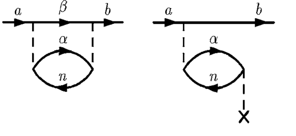
Figure 1: Some Goldstone diagrams representing a one-body core-valence correlation (left) and one-body subtraction diagram (right). Lines running left to right represent electrons, while lines running right to left are holes. $\ket{a}$ and $\ket{b}$ are valence orbitals, $\ket{\alpha}$ and $\ket{\beta}$ are virtual, and $\ket{n}$ is a hole in the core [6].

In addition to the standard core-valence MBPT, ambit can also include MBPT corrections to valence-valence integrals, as introduced in [2]. In this approach, the MBPT expansion in equation (13) includes additional diagrams representing correlations between highly-excited valence states (i.e. outside the upper-bounds of the CI-space $P$), as shown in figure 2.

Valence-valence MBPT is significantly computationally cheaper than including the orbitals directly in the full CI subspace. However, as with all MBPT techniques, care must be taken to ensure that there are no non-perturbative diagrams in the MBPT expansion. Specifically, including orbitals which are far from spectroscopic (such as orbitals with high orbital angular momentum) or orbitals which are close in energy to those in $P$ can produce non-perturbative diagrams with small energy-denominators. These diagrams can significantly reduce the accuracy of CI+MBPT calculations and are easy to inadvertently include in the MBPT expansion, so this approach should only be used with a carefully constructed MBPT subspace $Q$.

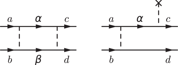
Figure 2: Two-body valence-valence diagram (left) and valence-valence subtraction diagram (right). External lines $a,b,c,d$ correspond to valence or hole orbitals in the CI subspace $P$, while the interior lines $\alpha$ and $\beta$ are virtual electron orbitals, at least one of which must not be valence for the intermediate state to be in $Q$ [2].

The energies for each calculated eigenstate are presented by ambit in ascending order of energy, grouped by total angular momentum $J$ and parity $\pi$. The solutions also contain the CI expansion coefficients and Landé g-factors, to aid in identifying levels. It is important to note that the absolute energies do not represent ionisation energies or any other physically meaningful quantity: the atom is effectively in a box due to the finite extent of the basis orbitals. Rather only the relative energies of the eigenstates (and the resulting atomic spectrum) represent physically meaningful quantities.

Finally, the resulting CI+MBPT wavefunctions are used to calculate transition matrix elements for electric and magnetic multipole operators, which we refer to as “external field” operators, as well as hyperfine dipole and quadrupole operators. ambit can calculate either reduced matrix elements $T$:

$$T_{if}=\bra{f}\hat{O}\ket{i}$$ (14)

for some operator $\hat{O}$, initial state $\ket{i}$ and final state $\ket{f}$, or line-strengths:

$$S_{if}=\left|T_{if}\right|^{2}$$ (15)

Transition matrix element calculations may additionally include frequency-dependent random-phase approximation (RPA) corrections [26, 27, 28]; detailed equations implemented in ambit are presented in Ref. [29].

4.2 Emu CI

The CI method outlined in section 4.1 relies on constructing and diagonalising the Hamiltonian matrix over a set of many-electron CSFs. The number of CSFs, and consequently the size of the CI matrix, scales exponentially with the number of electrons included in the CI problem subspace, resulting in prohibitively large CI matrices for systems with more than three valence electrons. Additionally, CI is slowly converging even for relatively simple systems with few valence electrons [30], making saturation in open-shell systems infeasible with current computational methods.

ambit implements a new approach that greatly reduces the computational difficulties associated with CI, which we refer to as emu CI [16] (as the structure of the resulting CI matrix resembles an emu’s footprint). This approach is especially well-suited to the common case where we are only interested in calculating a few of the lowest-lying energy levels and allows for the use of significantly larger CI basis sizes than would otherwise be possible. A schematic representation of this approach is shown in figure 3.

Emu CI relies on the fact that the CI expansion (10) is dominated by relatively few large contributions from off-diagonal CI matrix elements. Other CSFs contribute less strongly, and so interactions between these may be neglected. The shaded region of the matrix shown in figure 3 is formed as the Cartesian product of the $N_{\mathrm{CI}}$ CSFs in the CI-space $P$, which we refer to as the “large side” of the matrix, and a smaller set of $N_{\mathrm{small}}<N_{\mathrm{CI}}$ CSFs, which we refer to as the “small side” of the matrix. The small side contains a subset of CSFs that make the largest contribution to the CI expansion. Perturbation theory estimates performed in [31] show that the remaining off-diagonal terms, shown in white, produce a negligible contribution for the small number of states of interest, and can be set to zero without serious loss of accuracy.

The small-side CSFs are formed by allowing electron and/or hole-excitations from a set of leading configurations (which is not necessarily the same as used when forming the main CI-space) up to some maximum principal quantum number $n$ and orbital angular momentum $l$. This limit is specified using the same format of basis string used when forming the main CI-space. Finally, the small-side can be include an arbitrary number of electron- and hole-excitations (which also do not have to be the same as in the main CI-space).

We can then construct the CI matrix such that the significant off-diagonal terms are grouped together in a block, producing the structure shown in figure 3. These elements are further sorted such that the configurations with the largest number of corresponding projections appear first in the matrix to provide better performance when constructing and diagonalising the matrix in parallel.

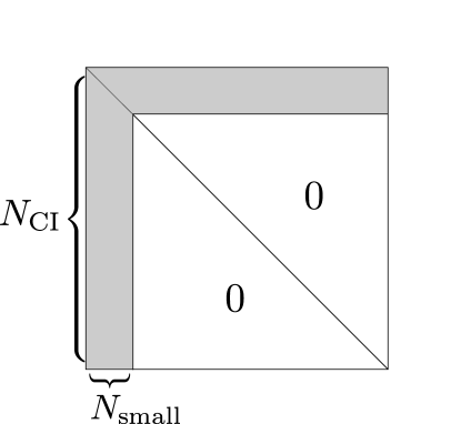
Figure 3: Structure of the CI matrix under the emu CI approximation. The $N_{\mathrm{CI}}\times N_{\mathrm{small}}$ nonzero off-diagonal terms are shaded in light grey, terms neglected in the approximation are shown in white

The dramatically reduced number of non-zero elements in the emu CI matrix compared to standard CI significantly reduces the computational resources required to obtain accurate atomic spectra. Recent calculations of the spectra of neutral tantalum and dubnium [16] shows that emu CI is capable of producing highly accurate atomic spectra for five-electron systems despite its relatively small resource usage. Spectra from these calculations were within $\sim\!10$% of experimental values, and convergence tests showed that the CI expansion was close to saturation. Similarly, applying this technique to the Cr⁺ calculations presented in this paper reduces the number of non-zero elements in the effective CI by a large factor. Even larger reductions in matrix size were used in [16]. The full matrices would be far to large to store in memory, even on modern high-performance computing clusters. Emu CI, combined with modern parallel programming techniques enables the use of extremely large CI bases, even for challenging open-shell systems with strong correlations.

5 Description of program components

The aspects of the CI+MBPT calculation presented in section 4 are controlled by a set of input options supplied to the software at run-time. This section contains a list of the most commonly used options when performing a full CI+MBPT calculation; a more comprehensive list can be found in the ambit user guide supplied with the software.

Input options are specified as either command-line arguments passed to the ambit executable, or contained in a plain-text input file. The input file must end with the suffix .input and be passed as a command line argument when calling the ambit executable. Although both input methods are equivalent and can be used interchangeably, we will assume that the input options are specified in an input file in this section.

Input options are organised into a series of sections loosely corresponding to the physical sections of the calculation outlined in section 4. Figure 4 provides a high-level overview of program flow, as well as the correspondence between input sections and physical methods.

Each section begins with a header in square brackets and continues until the next header (or end-of-file) and can contain any number of subsections of the form:

[Section]
Argument
[Section/Subsection]
Argument

Equivalently, sections and sub-sections may be included in a single-line argument with the format:

Section/Argument
Section/Subsection/Argument

The latter format can also be supplied as command line arguments when invoking ambit. These sections can occur in any order in the input.

Options in CamelCase (i.e. capitalisation denotes separate words) accept a value with the syntax Option = value. Options consisting of lower-case words separated by dashes (e.g. --check-sizes) are flags used to toggle behaviour on or off and do not accept values. Input options not specified as mandatory may be left out of the input and will default to values given in square brackets next to the option.

ambit will print all supplied arguments, as well as the current version, at the top of each calculation’s output; this ensures that any individual calculation can be exactly repeated using only information presented in the software output. In addition, the software saves the set of basis orbitals, one- and two-body MBPT integrals and atomic wavefunctions obtained by CI as binary files in the current working directory (i.e. the location from which the ambit executable is launched), allowing calculations to be cancelled and resumed, as well as for results from previous calculations to be reused in future calculations.

Most options specifying orbitals or configurations take non-relativistic inputs, which are automatically converted into the corresponding set of relativistic orbitals or configurations for use in the rest of the calculation.

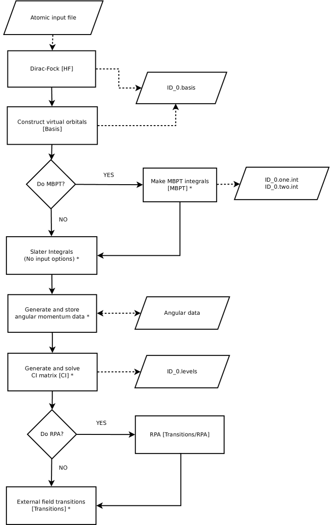
Figure 4: Flow chart representing control and program flow of ambit. Rectangular blocks represent physical sections of the calculation outlined in section 4, with the corresponding input file section (if any) listed in square brackets. Program sections labeled with an asterisk * are parallelised with MPI, OpenMP or both. Solid arrows represent program control flow, while dashed arrows represent input/output files consumed/created by ambit.

5.1 General options

The following general options do not fall under any named section of the input and must be specified at the beginning of the input file (i.e. before any named sections are introduced):

ID An identifier for the calculation, used to label the binary files generated during the calculation. (Mandatory.)

Z Atomic number of the atomic system. (Mandatory.)

-s1,2,3 Specifies which of the one-, two- or three-body MBPT diagrams to include in the calculation. Any combination of $1,2$ or $3$ may follow the -s, so e.g. -s1 will only calculate one-body MBPT corrections, while -s123 will calculate one-, two- and three-body corrections. No MBPT corrections will be calculated if no variations of this flag are set.

–no-new-mbpt Do not calculate any new MBPT integrals. Any integrals saved in .int files will still be read, however integrals that have been requested, but are not present in the .int files, will not be calculated.

NuclearInverseMass Inverse of the nuclear mass in atomic units: $1/M_{\mathrm{nuc}}$. Used to calculate isotopic mass-shift.

NuclearRadius Specifies the radius parameter of a Fermi distribution for nuclear charge. This value is used to compute the nuclear RMS radius, which is automatically used to calculate field-shift contributions. If either NuclearRadius = 0 or NuclearThickness = 0 are set then the nucleus is treated as a point charge.

NuclearThickness Specifies the density parameter of a Fermi distribution for nuclear charge. If either NuclearRadius = 0 or NuclearThickness = 0 are set then the nucleus is treated as a point charge.

–check-sizes Calculates and prints the number of MBPT and Coulomb integrals, as well as the number of CSFs per symmetry $J^{\pi}$ (i.e. the size of the CI matrices) without calculating any integrals or energy levels. Used to obtain a rough estimate of the size of the desired calculation before running it in full. This option will also calculate any angular data (if required), which can be computationally intensive and often requires ambit to be run in parallel to complete quickly.

5.2 [Lattice]

The [Lattice] input section specifies the parameters of the numerical lattice on which the basis functions and solutions are calculated. The lattice uses exponential spacing close to the nucleus and transitions to linear spacing at larger radii. Points in “real-space”, $r$, are related to the uniformly-spaced set of lattice-points $x$ by:

$$x=r+\beta\ln(r/r_{0})$$ (16)

where $r_{0}$ is the starting point of the lattice in atomic units (corresponding to Lattice/StartPoint) and $\beta$ controls the distance at which the lattice transitions from exponential to linear spacing.

[Lattice] contains the following options:

NumPoints[1000] Number of points in the lattice.

StartPoint[1.0e-6] Starting point of the lattice in atomic units. Must be nonzero.

EndPoint[50.0] Last point in the lattice (in real-space).

5.3 [HF] - Dirac-Hartree-Fock

The software allows for considerable freedom in specifying the Dirac-Hartree-Fock component of a calculation. In general, any number of electrons can be included in the procedure in any desired (valid) configuration. The choice of Dirac-Fock potential $V^{N_{\mathrm{DF}}}$ as described in section 4 can severely impact the accuracy of the resulting spectra; with a potential $V^{N_{\mathrm{DF}}}=V^{N}$ producing “spectroscopic” core orbitals (which benefit CI convergence) but potentially introducing large subtraction diagrams for open-shell systems (which can reduce MBPT accuracy).

Additionally, the Dirac-Hartree-Fock section of the calculation allows for the inclusion of a number of “decorators”, such as the Breit interaction or QED corrections, which modify the Dirac-Fock operator. Decorators introduced in this step of the calculation persist for the lifetime of a particular run of ambit, and are also incorporated in the CI (Slater) and MBPT integrals. These decorators are controlled by flags passed to the [HF] section of the input file.

The [HF] section accepts the following arguments and flags:

N The number of electrons to include in the Dirac-Fock procedure. (Mandatory.)

Configuration String specifying the nonrelativistic configuration to be included in the Dirac-Fock calculations (can include valence as well as core electrons). The Fermi level can be specified with a colon (‘:’), orbitals above which will be included in the CI and MBPT valence space $P$. If no Fermi level is specified it will default to immediately above the highest supplied orbital in this argument. Additionally, Valence holes can only appear in shells with energy below the Fermi level.

As an example, the string HF/Configuration = ’1s2 2s2 2p6 : 3s1’ will include the configuration 1s² 2s² 2p⁶ 3s, with 1s, 2s and 2p shells below and 3s above the Fermi level. (Mandatory; configuration must have HF/N total electrons.)

–breit Decorator including effects of the Breit interaction.

–sms Decorator for Specific Mass Shift operator for isotope shift.

–nms Decorator for Normal Mass Shift operator for isotope shift.

5.4 [HF/QED] - QED corrections

The decorators incorporating the Lamb shift corrections to the atomic spectra are controlled by arguments in the [HF/QED] section of the input file, which accepts the following arguments:

–uehling Decorator for the Uehling (vacuum polarisation) correction.

–self-energy Decorator for the self-energy correction.

5.5 [Basis] - CI+MBPT basis functions

As outlined in Section 4.1, single-particle basis orbitals are obtained by diagonalising a large set of B-Splines against the Dirac-Fock operator. The B-Spline basis includes orbitals up to some maximum principal quantum number and orbital angular momentum as determined by the Basis/ValenceBasis or MBPT/Basis input arguments, whichever is higher. This input section also determines the extent of the CI space $P$. The CI basis will be constructed using electron orbitals between the Fermi level and the upper limit set by Basis/ValenceBasis and hole orbitals between the lower limit set by Basis/FrozenCore and the Fermi level.

Once the basis has been generated, it is saved to the binary file <ID>_0.basis (where <ID> is given by the corresponding input option in section 5.1) in the current working directory. The software checks for the existence of this file in the current working directory and will reuse any pre-calculated orbitals rather than generate a new set for each calculation.

The [Basis] section of the input file accepts the following arguments:

ValenceBasis String specifying the maximum principal quantum number, $n$, and orbital angular momentum, $l$, of the orbitals included in the CI space $P$. The electron orbitals included in CI will therefore run from the Fermi level up to the limit specified by this option. For example, Basis/ValenceBasis = 10spdf will include orbitals with $0\leq l\leq 3$ and $n\leq 10$ for each partial wave. It is also possible to specify different values of $n$ for each partial wave, so, for example, Basis/ValenceBasis = 10sp7d will include s- and p-orbitals with $n\leq 10$ and d-orbitals with $n\leq 7$. (Mandatory.)

FrozenCore Sets an upper limit to the frozen core, in which the shells cannot have holes. This argument accepts the same input syntax as Basis/ValenceBasis, so Basis/FrozenCore = 4sp3d will not allow holes in s- and p-shells with $n\leq 4$ and d-shells with $n\leq 3$. If this option is omitted then the frozen-core will be set at the Fermi level (i.e. no holes will be allowed in CI).

–bspline-basis Construct the basis functions from B-Splines.

5.6 [Basis/BSpline] - B-Spline options

While it is generally fine to use the default values for the low-level, mathematical properties of B-Splines used to generate the basis functions, it is also possible to directly set these properties with the arguments in this section. See refs. [22] and [23] for a full discussion of the use of B-Splines as basis functions.

N [40] Number of splines per basis function.

K [7] Order of splines (splines are polynomials of degree $k-1$ and are nonzero across $k$ intervals). Default value is 7, but this will be automatically adjusted so $k\geq l_{\mathrm{max}+3}$.

Rmax [50.0] Maximum radius of the B-Splines. This should be chosen so that valence orbitals are not seriously impacted by the truncation at finite radius.

SplineType [Reno] Specifies the boundary conditions used to eliminate spurious states from the basis. Options are Reno (the default) [23], NotreDame [22] or Vanderbilt [24].

5.7 [CI] - Configuration Interaction

The CI matrix eigenvalue problem is solved by one of two methods, depending on the size of the matrix and number of required solutions. For small matrices with less than $N=200$ CSFs, we simply solve the eigenproblem directly using an implementation of the LAPACK linear algebra library such as Intel’s MKL or Eigen (the latter is used by default in ambit).

Direct diagonalisation is prohibitively computationally expensive for larger matrices, however. If only a few ($<50$) solutions are required, ambit instead solves the CI problem with a Fortran implementation of Davidson’s algorithm [32] developed by Stathopoulos and Froese Fischer [33]. Davidson’s algorithm is an iterative, $\mathcal{O}(N^{2})$ algorithm which is rapidly convergent when only a few extreme (in this case, lowest-lying) eigenvalues and vectors are required. This is commonly the case in CI+MBPT calculations. Davidson’s algorithm does not modify the matrix elements during the solution and only requires matrix-vector multiplications, which can benefit from the internal parallelism of linear algebra libraries such as the MKL or Eigen, greatly reducing the time taken to solve the eigenproblem.

The resulting levels are grouped by total angular momentum $J$ and parity $\pi$, before being ordered by energy within each symmetry. The energy (in both atomic units and cm^-1), configuration percentages and Landé g-factors are then printed to standard output. A sample of this output for Cr⁺ calculations is shown below:

Solutions for J = 0.5, P = even (N = 204534):
0: -9.8305729    -2157561.36528 /cm
        4s1 3d3 14d1  1.3%
             4s1 3d4  89%
             5s1 3d4  2.8%
    g-factor = 3.331

1: -9.8021109    -2151314.67386 /cm
        4s1 3d3 13d1  1.1%
        4s1 3d3 14d1  1.6%
        4s1 3d3 15d1  1.1%
             4s1 3d4  88%
             5s1 3d4  2%
                 3d5  2%
    g-factor = 0.0028481

 ...

The resulting energy levels are also stored in the binary file <ID>_0.levels in the current working directory. The software will not generate any stored levels if this file exists prior to starting the calculation, but will calculate any additional requested levels.

The [CI] section of the input file accepts the following options and flags:

LeadingConfigurations List of all configurations from which to generate many-body CSFs for the Hamiltonian matrix. For example, CI/LeadingConfigurations=’4d5, 4d4 5s1’ will build the Hamiltonian matrix by exciting electrons or holes from the two listed configurations (4d⁵ and 4d⁴5s). The list can contain arbitrarily many leading configurations, but all configurations must conserve particle number and must explicitly specify the number of particles in each orbital. Holes in an otherwise filled shell (i.e. located below the Fermi level) are denoted by a negative occupation number, e.g. CI/LeadingConfigurations=’3d-1’ contains a hole in the 3d shell. (Mandatory.)

ExtraConfigurations List of “extra” configurations to be included in the CI matrix. No electron or holes will be excited from these configurations. Accepts a list of non-relativistic configurations with the same form as CI/LeadingConfigurations.

ElectronExcitations[2] Number of electron excitations to include in the CI procedure. Defaults to 2 if no value is specified. This option also accepts input as a string of the form ’1, <Size 1>, 2, <Size 2>, ...’, which specifies different limits on $pqn$ and $l$ for each electron. For example, the string CI/ElectronExcitations=’1,8spdf,2,6spd’ will include all single-excitations up to 8spdf and all double-excitations up to 6spd.

HoleExcitations[0] Number of hole excitations to include in the CI procedure. Takes similar input to CI/ElectronExcitations.

EvenParityTwoJ List of total angular momenta $2J$ of even parity to solve the CI problem for. For example, CI/EvenParityTwoJ=’0, 2, 4’ will generate and solve the Hamiltonian matrices for even parity states with $J=0,1,2$. (At least one of CI/EvenParityTwoJ, CI/OddParityTwoJ or CI/--all-symmetries must be specfied).

OddParityTwoJ List of total angular momenta $2J$ of odd parity to solve the CI problem for. For example, CI/OddParityTwoJ=’1, 3, 5’ will generate and solve the Hamiltonian matrices for odd parity states with $J=1/2,3/2,5/2$. (At least one of CI/EvenParityTwoJ, CI/OddParityTwoJ or CI/--all-symmetries must be specfied).

–all-symmetries Solves the CI eigenproblem for every available angular momentum of both parities.

NumSolutions[6] Number of eigenvalues to generate for each symmetry $J^{\pi}$.

–gfactors Calculate the Landé g-factors for each solution (this option is enabled by default unless CI/NumSolutions $>50$).

–no-gfactors Do not calculate g-factors (since this can take a long time for large $N_{CI}$).

5.8 [CI/SmallSide] - Emu CI

Small-side CI is enabled and configured in the sub-section [CI/SmallSide], which accepts the following options:

LeadingConfigurations List of leading configurations from which to generate the small-side of the emu CI matrix. Input syntax is as for CI/LeadingConfigurations. (Mandatory if using emu CI.)

ElectronExcitations Number of electron excitations to include in the “small side” of the matrix. This option accepts the same input format as CI/ElectronExcitations. The CI/SmallSide subsection is only useful when the “small side” of the matrix is smaller than that specified in CI, so it is important to ensure only the desired configurations are included here.

HoleExcitations[0] - Number of hole excitations to include when building the small-side of the Hamiltonian matrix.

ExtraConfigurations List of “extra” configurations to be included in the small side of the emu CI matrix. No electron or holes will be excited from these configurations. Accepts a list of non-relativistic configurations with the same form as CI/LeadingConfigurations.

5.9 [MBPT]

MBPT diagrams and corrections are only calculated if appropriate flags are passed to ambit; arguments specified in this section of the input will be ignored by the software unless the -s[123] flag has been passed as input.

Once the one- and two-body MBPT integrals have been calculated, they are then stored to disk in the current working directory as the binary files <ID>_0.one.int and <ID>_0.two.int, respectively. Three-body MBPT integrals are not stored, however, as the number of three-body integrals grows very rapidly with the number of orbitals included in MBPT. However each diagram is relatively inexpensive given a set of pre-calculated two-body integrals so it is not generally efficient to store them in full between calculations. Three-body MBPT diagrams are only included for Hamiltonian matrix elements where at least one CSF is drawn from the set of leading configurations. Both one- and two-body MBPT integrals are computationally intensive, so calculations for these both types of integrals are parallelised by MPI, with the two-body integrals being further parallelised by OpenMP.

Additionally, the MBPT expansion is carried out in the Brillouin-Wigner formalism, in which the energy denominators in equation 13 depend on the total energy of the valence electrons [6, 1]. While it is straightforward to use the energies obtained from Dirac-Fock for the valence energy, there is some computational freedom as to which orbitals to include in the denominators (see ref. [6] for a more detailed discussion of this point). In electron-only calculations, the software will default to using the orbitals immediately above the Fermi level specified by the input option HF/Configuration. However, shells which may contain holes in particle-hole calculations should be included in the energy denominators, in which case it is necessary to explicitly specify these orbitals via the MBPT/EnergyDenomOrbitals input argument.

Options for MBPT calculations are as follows:

Basis Upper limit on the principal quantum number $n$ and orbital angular momentum $l$ of virtual orbitals to include in MBPT diagrams. Input string is of the same form as Basis/ValenceBasis, so MBPT/Basis = 30spd20f will include all s-, p- and d-orbitals with $n\leq 30$ and f-orbitals with $n\leq 20$ (must be a superset of Basis/ValenceBasis).

–use-valence Include valence-valence MBPT diagrams for orbitals above the limit set in Basis/ValenceBasis and below MBPT/Basis.

EnergyDenomOrbitals Specifies which orbitals/shells to use when calculating the valence energy in the MBPT diagram energy denominators. Accepts an orbital string as input, so e.g. MBPT/EnergyDenomOrbitals = 5sp4df will use the $5s$, $5p$, $4d$ and $4f$ orbitals to calculate the valence energy.

5.10 [Transitions] - Matrix elements of external fields

ambit uses wavefunctions obtained from CI procedure to calculate matrix elements for multiple possible operators, which may be diagonal or non-diagonal (transition) matrix elements. In addition to including options in [Transitions] in a new (clean) CI+MBPT run, transition matrix elements can also be calculated using pre-existing solutions from previous calculations, which are stored in the <ID>_0.levels file.

Matrix elements for the following operators are supported by ambit:

• E1, E2, E3 - Electric dipole, quadrupole and octupole operators,

• M1, M2 - Magnetic dipole and quadrupole operators,

• HFS1, HFS2 - hyperfine dipole and quadrupole operators,

Each of the above can have a different set of requested transitions. In addition, the software will present either the reduced matrix elements $T=\big{<}f||\hat{O}||i\big{>}$ or line strengths $S=|T|^{2}$ for each operator $\hat{O}$, but not both. If no options are specified the line-strengths will be calculated.

There are two possible ways of requesting transitions: either a set of individual transitions, or all transitions involving levels below a specified energy threshold can be targeted. Individual transitions must be requested according to the scheme <2J><parity>:<N>, where 2J is an integer equal to twice the total angular momentum, parity is either e or o (even or odd) and N is the integer used to order the level in the CI output. For example, 0e:0 -> 2o:1 represents the transition from the lowest energy state with even parity and angular momentum $J=0$ to the second lowest-energy state with odd parity and angular momentum $J=1$). The transitions requested need not necessarily be the same for each multipole operator.

Options for each operator are specified in separate subsections, such as Transitions/E1/--reduced-elements. Each subsection accepts the same set of possible arguments, but the arguments need not be the same for each requested operator. The arguments accepted by each subsection are as follows:

MatrixElements List of specific transition matrix elements to calculate, e.g. Transitions/M1/MatrixElements = ’1e:0 -> 1e:1, 3o:2 -> 3o:4’. Diagonal matrix elements for operators of, e.g. hyperfine structure, may also be given in the form Transitions/HFS1/MatrixElements = ’2e:0, 4e:0’.

AllBelow [0.0] Calculates all matrix elements between states with energy less than the argument.

Frequency Frequency of the external field (in atomic units). Only used with EJ and MJ operators. If not specified the default is to use the Dirac-Fock transition frequency; RPA must then be recalculated for each transition.

–reduced-elements Calculate the reduced matrix elements $T$ rather than the line strengths $S=|T|^{2}$.

–print-integrals Prints the raw value of the nonzero reduced one-body matrix elements $\big{<}a||\hat{O}||b\big{>}$ for each pair of valence orbitals $a$ and $b$.

–rpa Include frequency-dependent RPA corrections to the transition matrix elements.

RPA/–no-negative-states Exclude basis states in the Dirac sea (i.e. negative energy states) from RPA corrections.

5.11 Parallelism and performance

ambit is highly optimised to take advantage of modern high-performance computing hardware and makes extensive use of modern parallel programming techniques. We employ a hybrid model of parallelism, which uses MPI to divide the workload between computational resources (such as nodes on an HPC cluster) and OpenMP threads to further subdivide the workload between cores on a single resource. This approach allows us a fine-grained control over the workload distribution to match the hardware and network topologies of a particular system, providing greater per-node performance than a pure MPI approach. More importantly, part of the CI matrix must be duplicated between MPI processes, so this hybrid MPI+OpenMP approach is significantly more memory-efficient than pure MPI.

Creating and diagonalising the CI matrix is by far the most computationally expensive part of most CI+MBPT calculations, so this part of the software has been extensively optimised for both run-time and memory usage. First, the CI matrix is divided up into “chunks”, each of which contains the CSFs from four relativistic configurations. These chunks are then distributed approximately evenly between MPI processes, each of which then calculates the elements of the chunk in parallel via OpenMP. Additionally, the matrix is sorted such that the configurations with the most projections appear first. These rows are the most expensive to calculate, so this ensures that the OpenMP workload for each process is well balanced.

Once the CI matrix chunks have been populated, the matrix is then solved via Davidson’s method [32, 33], which distributes the necessary matrix-vector multiplications approximately evenly among MPI processes. These matrix-vector multiplications are trivially parallelisable, so we exploit internal OpenMP parallelism provided by either Eigen or Intel MKL to further parallelise each MPI process’s workload. This results in a dramatic speedup in matrix diagonalisation: even CI matrices with $10^{5}$ CSFs on a side can usually be diagonalised in a few minutes on a mid-sized HPC cluster.

In addition to CI, we also parallelise generating the Slater (CI) and MBPT integrals, which can dominate the calculation run-time for one and two valence-electron systems with a very large basis. Landé g-factors and transition matrix elements are also parallelised.

Finally, it is important to ensure that the parallel workload is divided appropriately for the topology of the target machine; incorrect choice of parallelism can severely impact performance. Usually, it is best to have spawn MPI process per node and as many OpenMP threads as there are cores per node. This is not the default behaviour for many MPI implementations (including OpenMPI and IntelMPI), so it must be explicitly requested when running ambit. Note that some hardware architectures, such as those with non-uniform memory access (NUMA) nodes may be better served by other distributions of threads and processes.

6 Example calculation: Cr⁺

In this section, we present results of two full CI+MBPT calculations for the spectrum of Cr⁺ to demonstrate the usage and features of ambit. All input and output files for this calculation are included as appendices in the folder CrIIExample. Cr⁺ is a five-electron system which requires a large CI basis and both core- and valence-MBPT corrections in order to produce an accurate spectrum, making it a good test-case for the theoretical and computational techniques included in ambit.

The two calculations presented here represent two computational regimes: a relatively small-scale calculation which requires only a single workstation or compute server, as well as a much larger scale calculation taking better advantage of modern HPC architecture. Both sets of calculations utilise emu CI and demonstrate that this technique allows for significantly higher accuracy than previous, standard CI+MBPT calculations [8].

Energy levels from these calculations are shown in tables 1 and 2. Table 1 additionally details the contributions to the overall energy from CI, one-, two-, and three-body core-valence MBPT. These results are also compared with experimental spectra from [17].

6.1 Dirac-Fock and B-spline basis

All of the Cr⁺ calculations presented in this section were undertaken using a $V^{N}$ Dirac-Fock potential, including all 3d⁵ valence electrons in the DF potential. This choice of potential necessarily introduces subtraction diagrams to MBPT, but these did not significantly degrade the accuracy of the calculations due to the large-CI basis employed throughout. We generated a frozen core consisting of filled 1s, 2s, 2p, 3s and 3p shells and included 3d valence orbitals above the Fermi level, as described in section 5.3. Additionally, we generate all single-particle B-Spline orbitals up to 16spdf for pure CI and 30spdfg for MBPT using the $V^{N}$ Dirac-Fock operator.

The choice of $V^{N}$ potential produces 3d orbitals which are spectroscopic for the 3d⁵ configuration, but which are less accurate at treating the 3d⁴ 4s configurations. Forming 3d orbitals with five electrons results in a Dirac-Fock wavefunction which is less tightly bound to the nucleus and thus has higher energy than the corresponding 3d⁴ DF orbital. Although this means our calculations tend to underestimate the energy of the levels with 3d⁴ 4s configuration, we find that use of the $V^{N-1}$ potential is much more slowly convergent for the ground-state 3d⁵ wavefunction, resulting in significantly reduced accuracy compared to our choice of $V^{N}$ potential.

6.2 Small-scale calculation

Our small-scale calculation targets even-parity states with $J=1/2,3/2,5/2,7/2,9/2$ and forms the CI configuration electron excitations from the 3d⁵, 3d⁴4s and 3d⁴4d leading configurations. Additionally, we employ the emu CI technique in section 4.2 with a “large-side” formed from single- and double-excitations up to 16spdf, and a “small-side” formed from single- and double-excitations up to 5spdf. This choice of CI basis results in CI matrices with $\sim 10^{6}\times 10^{4}$ nonzero elements, the largest of which consisted of $440704\times 9449$ CSFs for $J=5/2$.

Table 1 shows a break-down of the effects of one- two- and three-body core-valence MBPT corrections with a basis of 30spdfg. As previously stated, these calculations use the $V^{N}$ potential, which necessarily introduces large subtraction diagrams into the MBPT expansion as outlined in section 4.1. As can be seen in the $\Sigma^{(1)}$ column of table 1, including the one-body subtraction diagrams significantly reduces the accuracy of the resulting spectra; the calculations no longer correctly identify even the $3d^{5}$ ground-state. However, including the two- and three-body MBPT corrections, shown in the $\Sigma^{(2)}$ and $\Sigma^{(3)}$ columns in table 1, restores and improves the accuracy of the calculations due to the partial cancellation of subtraction diagrams by two- and three-body terms [8].

Both CI-only and CI+MBPT calculations required less than 40GB of memory and less than 1 hour of compute time when distributed between 16 cores – well within the capabilities of a high-performance workstation or a single node of a typical HPC cluster. This calculation does not approach saturation of the CI basis since it is constrained to require only relatively modest computational resources. However once all core-valence MBPT diagrams have been included, the CI+MBPT energy levels shown in table 1 have an average error of less than 5%.

Table 1: Energy levels of Cr⁺ (in cm^-1) for small-scale emu CI calculation. The “large-side” of the matrix contains single- and double-excitations up to 16spdf, while the “small-side” contains single- and double-excitations up to 5spdf. The first and second columns give the nonrelativistic configuration and approximate $LS$-coupling term for each calculated level. The CI column gives the (excitation) energies as calculated using a pure-CI approach, while the $\Sigma^{(1,2,3)}$ columns give the one-, two- and three-body MBPT corrections. Finally, the total energy and experimental energies obtained from ref. [17] are presented along with the percentage differences between experiment and our calculations.

Configuration	Term	CI	$\Sigma^{(1)}$	$\Sigma^{(2)}$	$\Sigma^{(3)}$	Total	Expt	$\Delta_{\mathrm{Expt.}}$ (%)
3d5	${}^{6}S_{5/2}$	0	0	0	0	0	0	–
3d4 4s	${}^{6}D_{1/2}$	14038	-15449	12116	2038	12742	11962	-6.5
3d4 4s	${}^{6}D_{3/2}$	14087	-15432	12102	2039	12795	12033	-6.3
3d4 4s	${}^{6}D_{5/2}$	14186	-15420	12087	2040	12893	12148	-6.1
3d4 4s	${}^{6}D_{7/2}$	14446	-15488	12129	2037	13124	12304	-6.7
3d4 4s	${}^{6}D_{9/2}$	14813	-15619	12218	2035	13448	12496	-7.6
3d4 4s	${}^{4}D_{1/2}$	20285	-14470	11807	2319	19941	19528	-2.1
3d4 4s	${}^{4}D_{3/2}$	20415	-14478	11801	2321	20060	19631	-2.2
3d4 4s	${}^{4}D_{5/2}$	20707	-21512	18797	2323	20315	19798	-2.6
3d4 4s	${}^{4}D_{7/2}$	21104	-22146	19389	2323	20671	20024	-3.2

6.3 Large-scale calculation

The large-scale calculation targets the same $J^{\pi}$ symmetries as the small-scale calculation, but employs a more sophisticated method of constructing the CI matrix. Here, we form the large-side from all single- and double- excitations from the 3d⁵, 3d⁴4s and 3d⁴4d leading configurations up to 15spdf. We then form the small-side from all single-excitations up to 15spdf and single- and double-excitations up to 5spdf. This approach more accurately captures the important configurations in the CI expansion at the expense of significantly larger matrix sizes. See listing 6.3 for the full input file used to generate the emu CI-only spectrum. The largest matrix ($J=5/2$) has $374944\times 109779$ non-zero elements and requires approximately 550GB of memory, which, while large, is still much less than full-CI and is still within the capabilities of modern HPC clusters.

Table 2 shows the calculated spectra from these large-scale CI-only calculations, as well as the effects of core-valence MBPT with a basis of 30spdfg. The CI-only calculations in table 2 give excellent agreement with experiment, with average errors at the $1\%$ level. However, unlike the smaller calculations (and CI+MBPT calculations from other codes), the inclusion of MBPT slightly degrades the calculation’s accuracy. Further increasing the size of the MBPT basis via the MBPT/Basis does not increase the accuracy beyond that of the CI-only calculation. This behaviour suggests that CI+MBPT has qualitatively different convergence at regimes close to saturation of the CI expansion for open-shell atoms, so care must be taken when using large-scale calculations for these systems.

Table 2: Energy levels of Cr⁺ (in cm^-1) for large-scale emu CI calculation. The “large-side” of the matrix contains single- and double-excitations up to 16spdf, while the “small-side” contains single-excitations up to 15spdf and single- and double-double-excitations up to 5spdf. The first and second columns give the nonrelativistic configuration and approximate $LS$-coupling term for each calculated level. The $E_{\mathrm{CI}}$ and $\Delta_{\mathrm{CI}}$ columns give the (excitation) energies and difference from experimental values as calculated using a pure-CI approach. The $E_{\mathrm{MBPT}}$ and $\Delta_{\mathrm{MBPT}}$ columns show the same comparison for CI+MBPT. The experimental values [17] are shown under $E_{\mathrm{Expt}}$.

Configuration	Term	ECI	$\Delta_{\mathrm{CI}}$ (%)	ECI+MBPT	$\Delta_{\mathrm{CI+MBPT}}$ (%)	$E_{\mathrm{Expt}}$
3d5	$6S_{5/2}$	0	–	0	–	0
3d4 4s	$6D_{1/2}$	11956	0.05	11237	6.1	11962
3d4 4s	$6D_{3/2}$	12072	-0.3	11341	5.7	12033
3d4 4s	$6D_{5/2}$	12265	-1.0	11512	5.2	12148
3d4 4s	$6D_{7/2}$	12531	-1.8	11750	4.5	12304
3d4 4s	$6D_{9/2}$	12867	-3.0	12048	3.6	12496
3d4 4s	$4D_{1/2}$	19441	0.4	19605	-0.4	19528
3d4 4s	$4D_{3/2}$	19624	0.04	19771	-0.7	19631
3d4 4s	$4D_{5/2}$	19921	-0.6	20043	-1.2	19798
3d4 4s	$4D_{7/2}$	20320	1.5	20398	1.9	20024

AMBiT input file used to generate Cr⁺ emu CI spectra in table 2.

ID=CrII
Z=24

[Lattice]
NumPoints=1000
StartPoint=1.0e-6
EndPoint=60.0

[HF]
N=23
Configuration=’1s2 2s2 2p6 3s2 3p6 : 3d5’

[Basis]
--bspline-basis
ValenceBasis=15spdf
FrozenCore=3sp
BSpline/Rmax=60.0

[CI]
LeadingConfigurations=’3d5, 3d4 4s1, 3d4 4p1’
ElectronExcitations=2
HoleExcitations=0
EvenParityTwoJ=’1, 3, 5, 7, 9, 11’
NumSolutions=6

[CI/SmallSide]
LeadingConfigurations=’3d5, 3d4 4s1, 3d4 4p1’
ElectronExcitations=’1,15spdf, 2,5spdf’

7 Acknowledgements

We thank A. J. Geddes for feedback and testing for ambit  as well as reviewing this manuscript. The work of EVK was supported by the Australian Government Research Training Program scholarship. The work of JCB was partially funded by the Australian Research Council grant DE120100399.

References

- [1] V. A. Dzuba, V. V. Flambaum, M. G. Kozlov, Combination of the many-body perturbation theory with the configuration-interaction method, Phys. Rev. A 54 (1996) 3948.
- [2] J. C. Berengut, Particle-hole configuration interaction and many-body perturbation theory: Application to Hg+, Phys. Rev. A 94 (2016) 012502.
-
[3]
F. Torretti, A. Windberger, A. Ryabtsev, S. Dobrodey, H. Bekker, W. Ubachs,
R. Hoekstra, E. V. Kahl, J. C. Berengut, J. R. C. López-Urrutia, O. O.
Versolato, Optical
spectroscopy of complex open--shell ions Sn7+ - Sn10+,
Phys. Rev. A 95 (2017) 042503.
doi:10.1103/PhysRevA.95.042503.
URL https://link.aps.org/doi/10.1103/PhysRevA.95.042503 -
[4]
M. G. Kozlov, S. G. Porsev, M. S. Safronova, I. I. Tupitsyn,
CI-MBPT:
A package of programs for relativistic atomic calculations based on a method
combining configuration interaction and many-body perturbation theory,
Computer Physics Communications 195 (2015) 199 – 213.
doi:doi:10.1016/j.cpc.2015.05.007.
URL http://www.sciencedirect.com/science/article/pii/S001046551500185X -
[5]
S. Fritzsche, C. Fischer, G. Gaigalas,
RELCI:
A program for relativistic configuration interaction calculations, Computer
Physics Communications 148 (1) (2002) 103 – 123.
doi:http://dx.doi.org/10.1016/S0010-4655(02)00463-0.
URL http://www.sciencedirect.com/science/article/pii/S0010465502004630 - [6] J. C. Berengut, V. V. Flambaum, M. G. Kozlov, Calculation of isotope shifts and relativistic shifts in CI, CII, CIII, and CIV, Phys. Rev. A 73 (2006) 012504.
-
[7]
I. M. Savukov,
Configuration-interaction
many-body-perturbation-theory energy levels of four-valent si i, Phys. Rev.
A 91 (2015) 022514.
doi:10.1103/PhysRevA.91.022514.
URL https://link.aps.org/doi/10.1103/PhysRevA.91.022514 -
[8]
J. C. Berengut, Isotope
shifts and relativistic shifts of Cr II for the study of variation
in quasar absorption spectra, Phys. Rev. A 84 (2011) 052520.
doi:10.1103/PhysRevA.84.052520.
URL http://dx.doi.org/10.1103/PhysRevA.84.052520 -
[9]
J. C. Berengut, V. V. Flambaum, M. G. Kozlov,
Isotope shift
calculations in Ti II, Journal of Physics B: Atomic, Molecular and Optical
Physics 41 (23) (2008) 235702.
doi:10.1088/0953-4075/41/23/235702.
URL http://stacks.iop.org/0953-4075/41/i=23/a=235702 -
[10]
J. Jiang, J. Mitroy, Y. Cheng, M. W. J. Bromley,
Relativistic
semiempirical-core-potential calculations of Sr+ using laguerre and
slater spinors, Phys. Rev. A 94 (2016) 062514.
doi:10.1103/PhysRevA.94.062514.
URL https://link.aps.org/doi/10.1103/PhysRevA.94.062514 - [11] P. Jonsson, G. Gaigalas, J. Bieron, C. Fischer, I. Grant, New version: Grasp2k relativistic atomic structure package, Computer Physics Communications 184 (9) (2013) 2197–2203.
-
[12]
J. Desclaux,
A
multiconfiguration relativistic dirac-fock program, Computer Physics
Communications 9 (1) (1975) 31 – 45.
doi:https://doi.org/10.1016/0010-4655(75)90054-5.
URL http://www.sciencedirect.com/science/article/pii/0010465575900545 -
[13]
M. F. Gu, The
flexible atomic code, Canadian Journal of Physics 86 (5) (2008) 675–689.
doi:10.1139/p07-197.
URL http://www.nrcresearchpress.com/doi/abs/10.1139/p07-197 - [14] V. A. Dzuba, V. V. Flambaum, Exponential Increase of Energy Level Density in Atoms: Th and Th II, Phys. Rev. Lett. 104 (2010) 213002.
-
[15]
V. A. Dzuba,
potential for atomic calculations, Phys. Rev. A 71 (2005) 032512.
doi:10.1103/PhysRevA.71.032512.
URL https://link.aps.org/doi/10.1103/PhysRevA.71.032512 -
[16]
A. J. Geddes, D. A. Czapski, E. V. Kahl, J. C. Berengut,
Saturated-configuration-interaction
calculations for five-valent Ta and Db, Phys. Rev. A 98 (2018) 042508.
doi:10.1103/PhysRevA.98.042508.
URL https://link.aps.org/doi/10.1103/PhysRevA.98.042508 -
[17]
A. Kramida, Y. Ralchenko, J. Reader, NIST ASD Team,
NIST Atomic Spectra Database (v5.4)
(2016).
URL http://physics.nist.gov/asd - [18] W. R. Johnson, Atomic Structure Theory : lectures on atomic physics, Springer, Berlin ; London, 2007.
- [19] V. V. Flambaum, J. S. M. Ginges, Radiative potential and calculations of qed radiative corrections to energy levels and electromagnetic amplitudes in many-electron atoms, Phys. Rev. A 72 (2005) 052115.
- [20] J. S. M. Ginges, J. C. Berengut, Atomic many-body effects and Lamb shifts in alkali metals, Phys. Rev. A 93 (2016) 052509.
- [21] J. S. M. Ginges, J. C. Berengut, QED radiative corrections and many-body effects in atoms: vacuum polarization and binding energy shifts in alkali metals, J. Phys. B 49 (2016) 095001.
- [22] W. R. Johnson, S. A. Blundell, J. Sapirstein, Finite basis sets for the Dirac equation constructed from B splines, Phys. Rev. A 37 (1988) 307.
- [23] K. Beloy, A. Derevianko, Application of the dual-kinetic-balance sets in the relativistic many-body problem of atomic structure, Comp. Phys. Commun. 179 (2008) 310.
-
[24]
C. F. Fischer, F. A. Parpia,
Accurate
spline solutions of the radial dirac equation, Physics Letters A 179 (3)
(1993) 198 – 204.
doi:https://doi.org/10.1016/0375-9601(93)91138-U.
URL http://www.sciencedirect.com/science/article/pii/037596019391138U - [25] M. G. Kozlov, S. G. Porsev, Effective Hamiltonian for valence electrons of an atom, Opt. Spectrosc. 87 (1999) 352.
-
[26]
W. R. Johnson, C. D. Lin, K. T. Cheng, C. M. Lee,
Relativistic
random-phase approximation, Physica Scripta 21 (3-4) (1980) 409.
URL http://iopscience.iop.org/1402-4896/21/3-4/029 -
[27]
V. A. Dzuba, V. V. Flambaum, O. P. Sushkov,
Relativistic many-body
calculations of the hyperfine-structure intervals in caesium and francium
atoms, Journal of Physics B: Atomic and Molecular Physics 17 (10) (1984)
1953.
URL http://stacks.iop.org/0022-3700/17/i=10/a=005 -
[28]
V. Dzuba, V. Flambaum, P. Silvestrov, O. Sushkov,
Shielding
of an external electric field in atoms, Physics Letters A 118 (4) (1986) 177
– 180.
doi:https://doi.org/10.1016/0375-9601(86)90251-3.
URL http://www.sciencedirect.com/science/article/pii/0375960186902513 -
[29]
V. A. Dzuba, J. C. Berengut, J. S. M. Ginges, V. V. Flambaum,
Screening of an
oscillating external electric field in atoms, Phys. Rev. A 98 (2018) 043411.
doi:10.1103/PhysRevA.98.043411.
URL https://link.aps.org/doi/10.1103/PhysRevA.98.043411 - [30] M. W. J. Bromley, J. Mitroy, Convergence of partial wave expansion of the He ground state, Int. J. Quantum Chem. 107 (2007) 1150.
- [31] V. A. Dzuba, J. C. Berengut, C. Harabati, V. V. Flambaum, Combining configuration interaction with perturbation theory for atoms with a large number of valence electrons, Physical Review A 95 (1) (2017) 012503.
- [32] E. R. Davidson, The iterative calculation of a few of the lowest eigenvalues and corresponding eigenvectors of large real-symmetric matrices, J. Comp. Phys. 17 (1975) 87.
- [33] A. Stathopoulos, C. Froese Fischer, A davidson program for finding a few selected extreme eigenpairs of a large, sparse, real, symmetric matrix, Comput. Phys. Commun. 79 (1994) 268.