Multifractal topography of several planetary bodies in the Solar System

Résumé

Topography is the expression of both internal and external processes of a planetary body. Thus hypsometry (the study of topography) is a way to decipher the dynamic of a planet. For that purpose, the statistics of height and slopes may be described by different tools, at local and global scale. We propose here to use the multifractal approach to describe fields of topography. This theory both encompass height and slopes and other statistical moment of the field, tacking into account the scale invariance. Contrary to the widely used fractal formalism, multifractal is able to describe the intermittency of the topography field. As we commonly observe the juxtapostion of rough and smooth at given scale, the multifractal framework seems to be appropriate for hypsometric studies. Here we analyze the data at global scale of the Earth, Mars, Mercury and the Moon and find that the statistics are in good agreement with the multifractal theory for scale larger than $\sim 10km$. Surprisingly, the analysis shows that all bodies have the same fractal behavior for scale smaller than $\sim 10km$. We hypothesized that dynamic topography of the mantle may be the explanation at large scale, whereas the smaller scales behavior may be related to elastic thickness.

(1) GEOPS, Univ. Paris-Sud, CNRS, Université Paris-Saclay, Rue du Belvédère, Bât. 504-509, 91405 Orsay, France (2) McGill University

1 Introduction

Scaling of coastlines was empirically studies by Richardson (1961), and Mandelbrot (1967) interpreted his reuslts in terms of fractals. Fractals are geometric sets of points that have a scale symmetry. Geophysical examples of scaling include turbulent phenomena including clouds, the wind, the ocean river flows, as well as various solid earth fields including rock faults and topography. Most systems of geophysical interest are mathematical fields, not geometric sets. When scaling, they will generally be multifractals. A general way to quantify this is to determine the statistical moments of fluctuations of the field, (generalized) structure functions. Denoting the fluctuation in the topography over a distance $\varDelta x$ by $\varDelta h$($\varDelta x$), the $qth$ order structure function is $\left\langle\varDelta h(\varDelta x)^{q}\right\rangle$. If the sytem is scaling, then this is a power law of the lag $\varDelta x$ : $\varDelta x^{\zeta(q)}$. The field is monofractal if $\zeta(q)=qH$ where H is named in honour of Hurst; in this linear case the field is quasi-Gaussian. In the more general multifractal case, $\zeta(q)=qH-K(q)$ where $K(q)$ is a convex function with $K(1)=0$, it determines the multifractality, the intermittency, the “spikeness” of the field. Numerous studies haves shown that in several context, topography is scaling on a significant range of scales.

For multifractal processes, local estimates of fractal dimensions will be different from one location to another, they will be stochastic. It is thus possible to interpret the topography of regions with quite different slope distributions in a unified multifractal framework. This suggests that even a global analysis of the topography of a planet might be scaling and multifractal despite of its diversity and complexity. Previous studies have established that the Earth’s topography is to a good approximation multifractal over a very wide range of scales (Lavallee et al., 1993; Gagnon et al., 2006). In the general case, $\zeta(q)$ is a concave function; in order to characterize or model multifractals one takes advantage of the existence of stable, attractive statistical behaviour: universality classes (Schertzer and Lovejoy, 1987).

In a previous analysis, we performed a global analysis on the topographic MOLA data from Mars (Smith et al., 2001). We also find a good agreement with universal multifractals but we found two scaling ranges with different characteristics (Landais et al., 2015). The statistical structure was found to be different at small scales (nearly monofractal) and large scales (multifractal) with a transition occurring at around $10km$. This behavior has been confirmed recently with other analyses (Deliege et al., 2016).

The goal of this article is to extend this pioneering Martian work to all planetary bodies whose topography is well estimated: the Earth, the Moon and Mercury. There is topography data for Venus and Titan but unfortunately too much data is missing to have a similar analysis on the global scale.

2 Universal multifractal theory

We first define the fluctuations $\varDelta h$($\varDelta x$). The simplest definition is the altitude differences, the slopes multiplied by $\varDelta x$, the most natural indicator of roughness. But there are many others way to define fluctuations. Wavelets provide a general method. Indeed, their coefficients define fluctuations (with appropriate normalization). The simple altitude difference corresponds to the “poor man” wavelet and can be advantageously replaced by the Haar wavelet that is more accurate and is useful over a wider range of exponents ($-1<H<1$, rather than $0<H<1$ for differences, see Lovejoy (2014) and paragraph below for a precise definition of Haar fluctuations.

Statistical moments

We can compute any statistical moment $M_{q}$ of order $q$ define by:

$$M_{q}(\Delta x)=<\Delta h(\Delta x)^{q}>$$ (1)

With $<>$, denoting the statistical average. If $q=2,$ it simply correspond to the variance. In principle, every orders (even non-integer orders) must be computed to fully revealed the whole variability of the data. If the field is scaling, all the statistical moment are expected to follow a power-law with scale.

Multifractality

Scaling allows us to introduce two distinct statistical processes : monofractal and multifractal. For a detailed description of the formalism we apply in this study, the readers can refer to Lovejoy and Shertzer (2013) briefly summed up in Landais et al. (2015) . We now quickly recall the main notions here after.

• In the usual gaussian monofractal case the parameters $H$ is sufficient to describe the statistic of all the moments of order $q$ (equation 2). Ther is no intermittency, meaning that the roughness of the field is spatially homogenous despite of its fractal variability regarding to scales. For example, the value $H=0.5$ correspond to the classic Brownian motion. This kind of statistical object has proved to be relevant in many local and regional analysis of natural surfaces (Orosei et al., 2003; Rosenburg et al., 2011), at least on restricted ranges of scales but fails to give full account to the intermittency commonly observed on larger topographic datasets.

  $$M_{q}\sim\Delta x^{qH}$$ (2)

• In the multifractal case, $H$ is no more sufficient to fully describe the statistics of the moments of order $q$. An additional convex function $K(q)$ depending on $q$ is required (see eq. 3). The moment scaling function $K$ slightly modifies the scaling law of each moment. The consequence on the corresponding field appears clearly on simulations (Gagnon et al., 2006) : the field exhibit a juxtaposition of rough and small places that are clearly more realistic in the case of natural surfaces. Moreover, it is possible to restrain the generality of the function $K(q)$, considering only universal multifractals, a stable and attractive class proposed by Schertzer and Lovejoy (1987) for which the multifractality is completely determined by the mean intermittency $C_{1}=\left(\frac{dK(q)}{dq}\right)_{q=1}$ (codimension of the mean) and the curvature $\alpha$ of the function $K$, $\alpha=\frac{1}{C_{1}}\frac{d^{2}K(q)}{dq^{2}}$ (the degree of multifractality). In that case the expression of $K$ is simply given by equation 5.

  $$M_{q}\sim\Delta x^{qH-K(q)}$$ (3)

$$\xi(q)=qH-K(q)$$ (4)

$$K(q)=\frac{C_{1}}{\alpha-1}(q^{\alpha}-q)$$ (5)

We see that the monofractal case correspond to $(H\neq 0,C_{1}=0)$ or $(H\neq 0,C_{1}\neq 0,\alpha\rightarrow 0)$.

3 Dataset

The topography of a planet is defined as the difference between the distance of the planetary surface and the geoid. For Mars (Smith et al., 2001), Mercury (Cavanaugh et al., 2007) and the Moon (Smith et al., 2010), we are used topographic data stored in PDS (http://pds-geosciences.wustl.edu) whereas the Earth data (Amante and Eakins, 2009) are gathered from numerous global and regional data sets. Table 1 sums up the main characteristics of the datasets. Each has already been previously analysed.

The Earth has been studied for multifratal purpose by Gagnon et al. (2006) using ETOPO5 dataset. They proposes to analyse separately continents and ocean and found that $H$ is varying from 0.46 for bathymetry and 0.66 for continent. The dataset considered in our study (ETOPO1, Amante and Eakins, 2009) is an arc-minute global relief model of the Earth.

On Mars, the main source of topographic data is the Laser altimeter MOLA (Smith et al., 2001) that allowed to perform extensive statistical analysis with different roughness indicators on sliding windows revealing interesting correlation with geological units (Aharonson et al., 2001; Kreslavsky and Head, 2000). The monofractal scaling of the topography of Mars has also been studied by Orosei et al. (2003) through the local computation of the scale independent Hurst parameters revealing a high disparity of values across the martian surfaces as expected for multifractal topography.

On the Moon, the high-precision topographic data obtained by the laser altimeter LOLA (Smith et al., 2010) has been extensively used. Kreslavsky et al. (2013) computed maps of roughness at hectometer and kilometer scales revealing poor correlations between these two scales. Moreover, Rosenburg et al. (2011) measured $H$. They not only identified a transition that occurs around 1km at most location but they also found significantly different values of $H$ in the Highlands ($H=0.95$) and in the Marias ($H=0.76$).

On Mercury, by using the MLA data (Cavanaugh et al., 2007), Pommerol et al. (2012) computed roughness indicators on extracted profiles from geologically distinct regions. Due to the eccentricity of the orbit, only the northern hemisphere could be mapped by laser altimetry with a resolution of about 5 kilometers. The use of pairs of stereoscopic images has finally made possible to develop an overall map of the topography of Mercury (Solomon et al., 2001; Hawkins et al., 2007). We analyzed both MLA data only and the full map (from both laser and stereoscopy) and found no significant difference, except the fact that larger scale are available for the full map. We thus choose to present here the full map only. This result confirm that there is no significant bias (at least with on multifractal properties) between stereoscopic and laser altimetric techniques.

The current study proposes to extend the scope of the multifractal analysis already performed on Earth and Mars (Gagnon et al., 2006; Landais et al., 2015) to all the bodies in the solar system for data is adequate . Thus the case of Earth, Mars, Moon and Mercury will be comparatively discussed. The case of Venus is not considered here despite of the existence of a dataset collected by Magellan because of the relative lack of topographic data comparing to the other bodies (Ford et al., 2014). The case is equivalent for Titan (Stiles et al., 2009).

	source	radius (km)	Resolution	min scale	max scale	lines	columns	nb fluctuations
Earth	ETOPO1	6371	60 pix/deg	1 853 m	20 015 km	10 800	21 600	0.2 billions
Mars	MOLA	3390	128 pix/deg	462 m	10 650 km	22 528	46 080	1 billion
Moon	LOLA	1737	512 pix/deg	60m	5 457 km	92 160	184 320	13 billions
Mercury	MLA	2240	64 pix/deg	665 m	7 037 km	11 520	23 040	0.0002 billion

Table 1: Characteristics of the datasets

4 Methodology

In our previous analysis (Landais et al., 2015), we considered the 1-D topographic profiles directly extracted from the along-track measurement of MOLA stored in PDS (http://pds-geosciences.wustl.edu, Smith et al. 2001). As the data are irregularly sampled due to the presence of clouds and instrument problems, we used multifractal simulations to study the effect of a MOLA-like irregular signal on the Haar fluctuations . It turned out that, most probably due to the small fraction of missing data, the irregularity had no detectable impact on the analysis. We also found that the use of the gridded data also produced the same results has the direct use of the more reliable along-track measurement, the conclusion being that for the purpose of a global analysis, the extrapolated gridded map for each body is sufficient to recover the global statistical parameters. The methodology used here is therefore much simpler and only relies on the gridded data . We only considered 1D North-South profiles and computed the Haar fluctuations at different lags $\Delta x$. The simplification to 1-D is reasonable as we perform a global statistical analysis. In addition, the North/South direction is more relevant than East-West because each profile as the same length. Figure 1a provides an example of 1-D profiles extracted from the gridded field for each body. See Landais et al. (2015) for a review of the different biases that could result from such an approach.

We implicitly consider that the global statistic are isotropic. This assumption is reasonable for the purpose of a global analysis given the fact that shape of various orientation can be found on a given body. Although local anisotropy is commonly observed (Kreslavsky and Head, 2003; Bondarenko et al., 2006; Bills et al., 2014), we assume it is erased by the spatial averaging. Isotropic multifractal processes readily produce strong local anistropy so that the question of systematic scale dependant statistical anisotropy is not easy to establish. Anisotropy remains an important issue and will be more carefully considered in future works

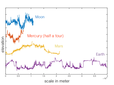
(a)

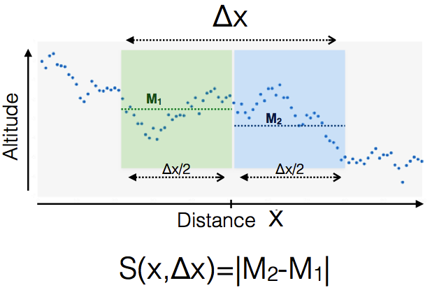
(b)

Figure 1: (a) Topographic dataset: 4 typical profiles, 1 for each body in the scope of this study. The length corresponds to 1 complete circumference of the planets except in the case of Mercury (only half a circumference) (b) Definition of the Haar fluctuation used to perform the statistical analysis. $M_{1}$ (respectively $M_{2}$) is the average of the first half (respectively second half) of the topographic profile.

Haar fluctuation and statistical moments

At a given location $x$ and a given scale $\varDelta x$ corresponding to $N$ successive elevation data on the grid, we average separately the first $\frac{N}{2}$ points $M_{1}(x,\varDelta x)$ and last $\frac{N}{2}$ points $M_{2}(x,\varDelta x)$. The Haar fluctuation is simply defined as the difference $S(x,\varDelta x)=\left|M_{2}(x,\varDelta x)-M_{1}(x,\varDelta x)\right|$. This definition is illustrated by figure 1b. The Mean Haar Fluctuation ($MHF$, moment of order 1) is simply obtained by averaging all the available haar fluctuations in a dataset. By extension, other statistical moments of any order q, $M_{q,HF}$ may be computed by averaging the fluctuations raised to the power of q :

$$MHF=<S(x,\varDelta x)>$$

$$MHF_{q}=<S(x,\varDelta x)^{q}>$$

5 Results for Earth, Mars, Mercury and the Moon

Mean Haar Fluctuations ($MHF$)

Figure 2 shows the Mean Haar Fluctuations ($MHF$, moment of order 1) for each body on a log-log plot. One can observe its scaling behavior as a function of the real distance (in meters). One can observe that at small scale, $MHF$ is from the larger to the smaller for : the Moon, Mercury, Mars, the Earth. This simply means that statistically, the roughness is from the larger to the smaller: for the Moon, Mercury, Mars, the Earth. Thus a astronaut (coming from the Earth) would experience topography differently by looking at the landscape of other planetary bodies. He would feel smaller in front of a rougher landscape at his/her scale. This feeling should be larger for the Moon. Another interesting features is the resemblance between i) the curves of Earth and Mars and ii) the curves the Moon and Mercury. For the two small bodies, the $MHF$ is clearly above the two others, except at the highest scales. By interpreting it as a roughness indicator, this feature simply reflects the well-known high level of roughness of small bodies, a consequence of intense craterisation shaping their surfaces.

As expected, the global $MHF$ increases with scale in all cases, simply reflecting the fact that larger scales yield larger differences in elevation. Nevertheless for the Earth and Mercury, at large scales, the $MHF$ begins to decrease before reaching its maximum scale. More specifically, as our goal is to study the global scaling behavior of topography, we expect this global increase of the $MHF$ to be linear on a log-log plot. It is clearly not the case on the entire available range of scales. Still noticeable scaling appears but over restricted ranges of scale : a transition seems to occur, separating two distinct scaling regimes. Such a transition is observed for all the bodies and interestingly, it occurs around 10-20 km in each case including the Moon. The nature of this transition discussed in our previous analysis focused on Mars and already pointed out by other authors in the case of Mars (Malamud and Turcotte, 2001), remains unknown.

On Figure 3, the $MHF$ are normalized by their respective values around 10 km in order to emphasize the transition at that scale. As one can see, the slope at small scales ($<10km$) are rather similar ($H\sim 0.8)$ whereas significantly different slopes are observed at large scales ($H\sim 0.2-0.5$). The scaling is excellent at large scales in the case of Mars and good in the case of Earth and Mercury. In the case of the Moon, data points are more dispersed, and $H$ might be less well defined. Note also at small scales, the available range for Earth and Mercury is limited and might result in an unconvincing fit. The values obtained for $H$ for each body by computing a linear regression on the distinct ranges of scale is reported on table 2.

Statistical moments $MHF_{q}$

In the case of universal multifractals, all the statistical moment will scale according to equation 3, the $MHF$ being the particular case for which $q=1$. Thus we can estimate the other multifractal exponents by computing statistical moments $MHF_{q}$ . On Figure 4, the $MHF_{q}$ are plotted for different values of q and for the different bodies. The next step is to compute linear regressions on every curve and on the distinct identified scaling regime. The log-log slopes $\zeta(q)$ may then be plotted as a function of $q$ for each body and for each range of scale (see Figure 5) in order to visualize the function $\xi$ defined by equation 4. A linear $\xi(q)$ is the signature of monofractality whereas a curved $\xi(q)$ indicates a multifractal behavior according to equation 2 and 3. Interestingly, Figure 5 clearly shows that on the distinct scaling regimes (low scale and large scales) the behavior is significantly different. On the range of small scales ($<10km$, plot on the left), the curves are rather similar for all the four bodies and very close to straight lines indicating that the statistics found to be roughly monofractal (small $C_{1}$) over the range. Over the range of large scales ($>10km$, plot on the right), we obtained curved structure functions in most cases revealing the multifractal nature of the statistics of topography over the range. The multifractal parameters are computed according to equation 3 and reported on table 2. Whereas the case of Mars, Mercury and Earth are similar of value of $C_{1}$ around 0.1, the case of the moon seems to be an exception with weak multifractal properties over that range of scales ($C_{1}$ close to 0).

scale<10km	Earth	Mars	Moon	Mercury
H	0.823 ± 0.004	0.773 ± 0.003	0.878 ± 0.002	0.922 ± 0.003
$\alpha$	NA	NA	NA	NA
$C_{1}$	0.01 ± 0.01	0.02 ± 0.006	0.02 ± 0.04	0.026 ± 0.005

scale>10km	Earth	Mars	Moon	Mercury
H	0.479 ± 0.001	0.53 ± 0.001	0.226 ± 0.002	0.248 ± 0.002
$\alpha$	1.70 ± 0.08	1.80 ± 0.06	1.4 ± 0.1	1.85 ± 0.1
$C_{1}$	0.093 ± 0.002	0.110 ± 0.002	0.03 ± 0.01	0.059 ± 0.002

Table 2: Estimations of multifractal parameters. NA stands for non-applicable. If the value of $C_{1}$ is very small (here <0.02), we can consider that the field is not multifractal and the value of $\alpha$ is not interpretable.

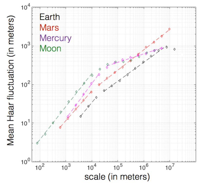
Figure 2: Mean Haar fluctuations $MHQ$ (order 1) as a function of scales for the 4 planetary bodies.

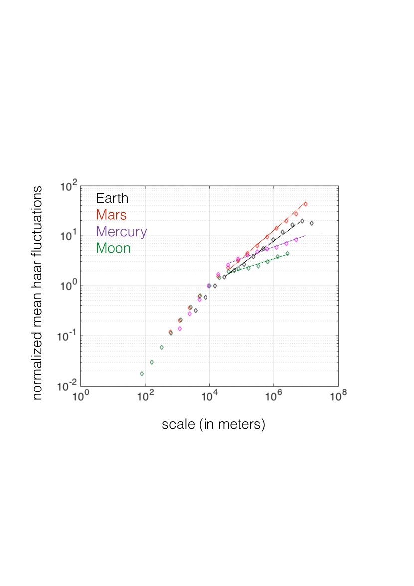
Figure 3: Mean Haar fluctuations normalized in order to be approximatively equal at scale 10km, as a function of scale. The normalization does not modify the scaling behavior from Fig. 2 but emphasize the transition that seems to occur around 10km.

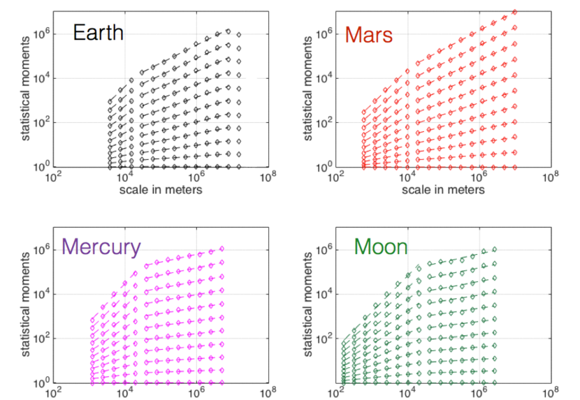
Figure 4: Plot of different statistical moments for the four bodies. The average fluctuations from figure 2 are shown as diamond whereas the moments of order 2 (average squared fluctuations) are triangles (top curves). In between are the non-integer order statistical moments. Although 21 moments have been computed for the purpose of this analysis (from 0.1 to 2 by steps of 0.1), only a few non-integers moments are plotted here for order 0.1 to order 2 by step of 0.2

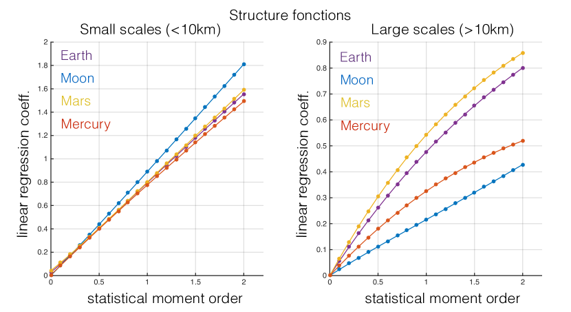
Figure 5: Structure function for different ranges of scales

6 Discussion and conclusion

By averaging the fluctuations at different scales, we have revealed global statistical pattern of planetary bodies. We tested and validated the multifractal approach on the four bodies with empirically well estimated topography : the Earth, Mars, Mercury and the Moon. We found that a transition occurs at about 10 km and that it is a general property of all planetary topographies. Below 10 km, differences in altitudes decrease more rapidly when the scale decreases.

As suggested by Araki et al. (2009) and Nimmo et al. (2011), for the transition in the power spectral density, we propose the interpretation that the elastic thickness of the lithosphere is responsible for this transition by acting against the deformations caused by the different surface processes in two regimes. At scales smaller than the elastic thickness $T_{e}$, a modification of the surface (for example, following an impact) does not make it possible to generate isostatic compensation. The new relief can therefore remain present. The slopes of neighboring facets tend to be correlated with each other and give rise to fluctuations in topography rapidly increasing with the scale (structured aspect, high $H$). The relief profile tends to be constructive since the slopes are highly correlated. At scales higher than $T_{e}$, a change in relief triggers an isostatic compensation which tends to oppose the large variations of the relief. The slopes of neighboring facets tend to be anti-correlated and the topographic profile is rougher. The relief oscillates around a mean value since the slope are more anti-correlated. In this configuration, the altitude fluctuations increase only slightly regarding to scale (low $H$). The common transition could be explained by the averaged value of the elastic thickness quite similar for the 5 bodies (Grott and Breuer, 2008; Barnett et al., 2000; Nimmo and Watters, 2004).

At scales larger than 10 km, all planetary bodies are different. Interestingly, the scaling law is characterized for the Moon by $H=0.2$, Mercury by $H=0.3$, Mars and Earth by $H=0.5$. The smaller the body, the less intense its internal activity due to intense thermal cooling. The value of $H$ may be related to its geological activity. One can speculate that a more intensively convecting mantle yields a higher value of $H$. This explanation links the large scale with dynamic topography (Hager et al., 1985). The fact that only large scale topography is strongly multifractal is coherent with this explanation because multifractal behavior is related to fluids mechanics and turbulent scale cascade. The geological origin of this transition will be investigated in future works.

From our result, this pattern seems coherent on large ranges of scale throughout the different bodies. Although suggesting that a few processes might operate simultaneously at different scales, this result is not incompatible with the existence of process operating at a specific altitude or locations. For example the “glacial buzz” saw effect seems limit the presence of high altitude on the Earth only (Lorenz et al., 2011). Our results simply suggest that the contribution of such process to global statistics can be neglected because if a strong altitude dependent process occurs, it should have broken the scaling behavior.

As a future work, we plan to perform local analysis on area defined by geological boundaries or altitude level to better understand the link between the scaling behavior of topography and natural processes operating at different location and altitude.

Annex : Bayesian regression

In order to estimate the best set of parameters $(H,\,C_{1},\alpha)$ modeling the data, the parameters can be estimated in a classical way by performing regressions on the function $\zeta$ near the mean $(q=1$) to quantify its curvature related to $\alpha$ and $C_{1}$ Lovejoy and Shertzer (2013) by the theoretical formulas:

$$H=\left.\frac{d\xi(q)}{dq}\right|_{q=1}\quad C_{1}=\left.\frac{dK(q)}{dq}\right|_{q=1}\quad\alpha=\left.-2\frac{d^{2}K(q)}{dq^{2}}\right|_{q=1}/\left.\frac{dK(q)}{dq}\right|_{q=1}$$ (6)

As a reminder, the scaling exponents $\zeta(q)$ are themselves the products of linear regression, so the fits from eq. 6 are only indirectly related the data. We wish to avoid this method which will not make possible to judge the quality of the estimates, especially as the multifractal component is rather weak when the function $\zeta(q)$ is only weakly curved.

We propose a new approach based on principle of Bayesian inversion (Tarantola and Valette, 1982) which allows to construct a posterior probability distribution of the parameters (mean, most probable value, standard deviation) from observations. In practice, these distributions can be estimated iteratively by applying the Metropolis rule to construct a Monte Carlo Markov chain (Mosegaard and Tarantola, 1995) containing the different sets of parameters. We summarize the main lines of this technique, already used on photometry problems (Schmidt and Fernando, 2015; Fernando et al., 2013). As a first step, it is necessary to evaluate the quality of the individual linear regressions of each moment. In this step, we attribute to each point an empirical uncertainty with a centered gaussian distribution. The latter will be the higher as the linear correlation through the scale is accurate. Then, we tested the direct model , computed by applying the laws of equations 4 and 4, for different random set of parameters $(H,\,C_{1},\alpha)$. Synthetic realizations are then compared to observations. The Monte Carlo Markov chain is created according the metropolis rules, using the likelyhood of empirical uncertainties. . This method allow us to estimated realistic uncertainty bars on parameter $(H,\,C_{1},\alpha)$, from the observational data (see table 2)