The truncated EM method for stochastic differential equations with Poisson jumps

Abstract

In this paper, we use the truncated EM method to study the finite time strong convergence for the SDEs with Poisson jumps under the Khasminskii-type condition. We establish the finite time $\mathcal{L}^{r}(r\geq 2)$ convergence rate when the drift and diffusion coefficients satisfy super-linear condition and the jump coefficient satisfies the linear growth condition. The result shows that the optimal $\mathcal{L}^{r}$-convergence rate is close to $1/(1+\gamma)$, where $\gamma$ is the super-linear growth constant. This is significantly different from the result on SDEs without jumps. When all the three coefficients of SDEs are allowing to grow super-linearly, the $\mathcal{L}^{r}(0<r<2)$ strong convergence results are also investigated and the optimal strong convergence rate is shown to be not greater than $1/4$. Moreover, we prove that the truncated EM method preserve nicely the mean square exponentially stability and asymptotic boundedness of the underlying SDEs with Piosson jumps. Several examples are given to illustrate our results.

1 Introduction

Due to the broad applications in modeling uncertain phenomenon, stochastic differential equations (SDEs) driven by Brownian motions have been attracting lots of attentions [1, 2]. When some unexpected events happen, some jumps may be needed to model the effects of those events. For example, a breaking news after the close of the stock market may lead to a huge difference between today’s closing price and tomorrow’s opening price. To take both the continuous and discontinuous random effects into consideration, SDEs driven by both Brownnian motions and Poisson jumps are often employed as a generalisation of the SDEs only driven by Brownian motions.

Despite the wide applications, the explicit solutions to SDEs are hardly found. Therefore, to construct some efficient numerical methods is of extremely important. The series works of Higham and Kloeden [3, 4, 5] studied some implicit methods for SDEs with Poisson jumps. In their papers, the strong convergence, the convergence rates and stability of different implicit methods were proposed and investigated for some SDEs, whose drift coefficient satisfies non-global Lipschitz condition, and both the diffusion coefficient and the coefficient for the Poisson jumps are global Lipschitzian. When the global Lipschitz condition on the diffusion coefficient is disturbed, the tamed Euler and the tamed Milstein methods were proposed for SDEs driven by the more generalised process, Lévy process [6, 7]. The taming techniques were original proposed in [8] for the construction of explicit methods for SDEs with non-globally Lipschitz continuous coefficients. As indicated in [9], explicit methods have their own advantages on the relatively simple structure and the avoidance of solving some nonlinear systems in each iteration. Therefore, the studies on explicit methods for SDEs with non-global Lipschitz coefficients have been blooming in recent years. Sine and cosine functions were employed in [10] to construct some explicit methods for SDEs with both the drift and diffusion coefficients growing super-linearly. The taming techniques were modified and generalised in [11] and [12]. The truncated Euler method were proposed in [13, 14].

In this paper, we borrow the truncating idea to propose the truncated Euler method for SDEs with Poisson jumps. The main contributions of this work are twofold. Firstly, all the drift coefficient, the diffusion coefficient and the coefficient for Poisson jumps are allowed to grow super-linear. To our best knowledge, this is the first work to study an explicit numerical method for SDEs with all the three coefficients that can grow super-linearly. Secondly, both the finite time convergence and asymptotic behaviours of the method are investigated.

It should be noted that the truncated Euler for SDEs with the global Lipschitzian pure jumps were studied in [15]. Other numerical methods for SDEs with Poisson jumps or Lévy process were also proposed and investigated [16, 17, 18, 19, 20], we just mention some of them here and refer the readers to the references therein. For the detailed and systemic introductions to numerical methods for SDEs and SDEs with jump, we refer the readers to the monographs [21] and [22].

This paper is constructed as follows. Section 2 sees some necessary mathematical preliminaries. Section 3 contain the main results on the finite time convergence. The asymptotic behaviours, stability and boundedness, of the numerical solutions are presented in section 4. Several examples are given in the Section 5. Section 6 concludes the paper and points out some future research.

2 Mathematical Preliminaries

Throughout this paper, unless otherwise specified, let $(\Omega,{\mathcal{F}},\mathbb{P})$ be a complete probability space with a filtration $\{{\cal F}_{t}\}_{t\geq 0}$ satisfying the usual conditions (i.e., it is increasing and right continuous while $\cal{F}_{\textrm{0}}$ contains all $\mathbb{P}$-null sets). Let $\mathbb{E}$ denote the probability expectation with respect to $\mathbb{P}$. Let $B(t)$ be an $m$-dimensional Brownian motion defined on the probability space and is $\cal{F}_{\textrm{t}}$-adapted. $N(t)$ is a scalar Poisson process with the compensated Poisson precess $\widetilde{N}(t)=N(t)-\lambda t$, where the parameter $\lambda$ is a jump intensity. If $A$ is a vector or matrix, its transpose is denoted by $A^{T}$. If $x\in\mathbb{R}^{d}$, then $|x|$ is the Euclidean norm. If $A$ is a matrix, its trace norm is denoted by $|A|=\sqrt{(A^{T}A)}$. For two real numbers $a$ and $b$, we use $a\vee b=\max(a,b)$ and $a\wedge b=\min(a,b)$. For a set $G$, its indicator function is denoted by $\mathbb{I}_{G}$. Moreover, $\mathcal{L}^{r}=\mathcal{L}^{r}(\Omega,{\mathcal{F}},\mathbb{P})$ denotes the space of random variables $X$ with a norm $|x|_{r}:=(\mathbb{E}|X|^{r})^{1/r}<\infty$ for $r>0$. In what follows, for notational simplicity, we use the convention that $C$ represents a generic positive constant, the value of which may be different for different appearances.

Consider a $d$-dimensional SDEs with Piosson jumps:

$$dx(t^{-})=f(x(t^{-}))dt+g(x(t^{-}))dB(t)+h(x(t^{-}))dN(t),\quad t\geq 0.$$ (2.1)

with the initial value $x(0)=x_{0}\in\mathbb{R}^{d}$, where $x(t^{-})$ denotes $\lim_{s\to t^{-}}x(s)$. Here, $f:\mathbb{R}^{d}\to\mathbb{R}^{d}$ is the drift coefficient, $g:\mathbb{R}^{d}\to\mathbb{R}^{d\times m}$ is the diffusion coefficient, $h:\mathbb{R}^{d}\to\mathbb{R}^{d}$ is the jumps coefficient.

3 Finite time convergence

3.1 Convergence rate of the partially truncated EM method in $\mathcal{L}^{r}(r\geq 2)$

In order to discuss the convergence rates of the truncated EM method in $L^{r}$ for $r\geq 2$. We assume that $f$ and $g$ can be decomposed as $f(x)=F_{1}(x)+F(x)$ and $g(x)=G_{1}(x)+G(x)$, where $F_{1},F:\mathbb{R}^{d}\to\mathbb{R}^{d}$, and $G_{1},G:\mathbb{R}^{d}\to\mathbb{R}^{d\times m}$. Moreover, the coefficients $F$, $G$, $F_{1}$ ,$G_{1}$ and $h$ satisfy the following conditions.

Assumption 3.1

There exist positive constant $L_{1}>0$ and $\gamma\geq 0$ such that

$$|F_{1}(x)-F_{1}(y)|\vee|G_{1}(x)-G_{1}(y)|\vee|h(x)-h(y)|\leq L_{1}|x-y|,\quad\forall x,y\in\mathbb{R}^{d}$$

$$|F(x)-F(y)|\vee|G(x)-G(y)|\leq L_{1}(1+|x|^{\gamma}+|y|^{\gamma})|x-y|,\quad\forall x,y\in\mathbb{R}^{d}.$$ (3.1)

The parameter $\gamma$, which we call super-linear growth constant. By Assumption 3.1, we can derive that there exists a positive constant $K_{1}$ such that

$$|F_{1}(x)|\vee|G_{1}(x)|\vee|h(x)|\leq K_{1}(1+|x|),\quad\forall x\in\mathbb{R}^{d},$$ (3.2)

which implies that $F_{1}$, $G_{1}$ and $h$ satisfy the linear growth condition. Similarly, we have

$$|F(x)|\vee|G(x)|\leq(2L_{1}+|F(0)|+|G(0)|)|x|^{1+\gamma},\quad\forall|x|\geq 1.$$ (3.3)

We also impose the following standing hypotheses.

Assumption 3.2

There exists a pair of constant $\bar{r}>2$ and $L_{2}>0$ such that

$$(x-y)^{T}(F(x)-F(y))+\frac{\bar{r}-1}{2}|G(x)-G(y)|^{2}\leq L_{2}|x-y|^{2},\quad\forall\;x,y\in\mathbb{R}^{d}.$$ (3.4)

By Assumption 3.2, we can derive that for any $r\in[2,\bar{r})$

$$(x-y)^{T}(f(x)-f(y))+\frac{r-1}{2}|g(x)-g(y)|^{2}\leq L_{3}|x-y|^{2}.$$ (3.5)

where $L_{3}=2L_{1}+L_{2}+\frac{L_{1}^{2}+(r-1)(\bar{r}-1)}{\bar{r}-r}$ (see [23]).

Assumption 3.3

(Khasminskii-type condition) There exist constants $\bar{p}>\bar{r}$, $K_{2}>0$ such that

$$x^{T}F(x)+\frac{\bar{p}-1}{2}|G(x)|^{2}\leq K_{2}(1+|x|^{2}),\quad\forall x\in\mathbb{R}^{d}.$$ (3.6)

By Assumption 3.3, we also have that for any $p\in[2,\bar{p})$

$$x^{T}f(x)+\frac{p-1}{2}|g(x)|^{2}\leq K_{3}(1+|x|^{2}),$$ (3.7)

where $K_{3}=2K_{1}+K_{2}+\frac{K_{1}^{2}+(p-1)(\bar{p}-1)}{\bar{p}-p}$ (see [23]).

The truncated idea is to deal with the super-linear coefficients. In the viewpoint of the finite-time convergence, the linear coefficient does not cause any problem to the EM scheme and hence there is no need to truncate it [23]. In our truncated EM method, we only truncate the super-linear terms, that is $F$ and $G$. To define the truncated EM scheme, we first choose a strictly increasing function $\mu:\mathbb{R}^{+}\rightarrow\mathbb{R}^{+}$ such that $\mu(n)\rightarrow\infty$, as $n\rightarrow\infty$, and

$$\sup_{|x|\leq n}|F(x)|\vee|G(x)|\leq\mu(n),\quad\forall n\geq 1.$$

Denoted by $\mu^{-1}$ is the inverse function of $\mu$. We also choose a strictly decreasing function $\varphi:(0,1)\rightarrow(0,\infty)$ such that

$$\lim_{\Delta\to 0}\varphi(\Delta)=\infty\quad\textrm{ and}\quad(\varphi(\Delta))^{\bar{p}}\leq\Delta^{-1}\wedge\Delta^{-\bar{p}/4},\quad\forall\Delta\in(0,1].$$ (3.8)

For a given step size $\Delta\in(0,1)$, let us define a mapping $\pi_{\Delta}$ from $\mathbb{R}^{d}$ to the closed ball $\{x\in\mathbb{R}^{d}:|x|\leq\mu^{-1}(\varphi(\Delta))\}$ by

$$\pi_{\Delta}=\big{(}|x|\wedge\mu^{-1}(\varphi(\Delta))\big{)}\frac{x}{|x|}.$$

We set $x/|x|=0$ when $x=0$. We then define the partially truncated functions

$$F_{\Delta}(x)=F(\pi_{\Delta}(x)),\quad G_{\Delta}(x)=G(\pi_{\Delta}(x)),\quad\forall x\in\mathbb{R}^{d}$$

$$f_{\Delta}(x)=F_{1}(x)+F_{\Delta}(x)\quad\textrm{and}\quad g_{\Delta}(x)=G_{1}(x)+F_{\Delta}(x),\quad\forall x\in\mathbb{R}^{d}$$

It is easy to see that

$$|F_{\Delta}(x)|\vee|G_{\Delta}(x)|\leq\varphi(\Delta),\quad\forall x\in\mathbb{R}^{d}.$$ (3.9)

Obviously, $F_{\Delta}$ and $G_{\Delta}$ are bounded while $F$ and $G$ may not. The following lemma shows that the truncated functions maintain the Khaminskii-type condition nicely (see [13]).

Lemma 3.4

Let Assumption 3.3 hold. Then, for all $\Delta\in(0,1]$, we have

$$x^{T}F_{\Delta}(x)+\frac{\bar{p}-1}{2}|G_{\Delta}(x)|^{2}\leq 2K_{2}(1+|x|^{2}),\quad\forall x\in\mathbb{R}^{d}.$$

We can show that for any $p\in[2,\bar{p})$ , we have

$$x^{T}f_{\Delta}(x)+\frac{p-1}{2}|g_{\Delta}(x)|^{2}\leq K_{4}(1+|x|^{2}),\quad\forall x\in\mathbb{R}^{d}.$$ (3.10)

where $K_{4}=2K_{1}+2K_{2}+\frac{K_{1}^{2}+(p-1)(\bar{p}-1)}{\bar{p}-p}$ (see [23]). We now form the discrete-time truncated EM numerical solutions $X_{\Delta}(t_{k}^{-})\approx x(t_{k}^{-})$, for $t_{k}^{-}=k\Delta t$ by setting $X_{\Delta}(0)=x_{0}$ and computing

$$X_{\Delta}(t_{k+1}^{-})=X_{\Delta}(t_{k}^{-})+f_{\Delta}(X_{\Delta}(t_{k}^{-}))\Delta t+g_{\Delta}(X_{\Delta}(t_{k}^{-}))\Delta B_{k}+h(X_{\Delta}(t_{k}^{-}))\Delta N_{k},\quad 0\leq k\leq M-1,$$ (3.11)

where $\Delta B_{k}=B(t_{k+1}^{-})-B(t_{k}^{-})$, $\Delta N_{k}=N(t_{k+1}^{-})-N(t_{k}^{-})$. It is consentient to use the continuous-time step process $\bar{x}_{\Delta}(t^{-})$ which is defined by

$$\bar{x}_{\Delta}(t^{-})=\sum_{k=0}^{\infty}X_{\Delta}(t_{k}^{-})\mathbb{I}_{[t_{k}^{-},t_{k+1}^{-})}(t)$$ (3.12)

where $\mathbb{I}$ is a indicator function. The other continuous-time process is defined by

$$x_{\Delta}(t^{-})=x_{0}+\int_{0}^{t}f_{\Delta}(\bar{x}_{\Delta}(s^{-}))ds+\int_{0}^{t}g_{\Delta}(\bar{x}_{\Delta}(s^{-}))dB(s)+\int_{0}^{t}h(\bar{x}_{\Delta}(s^{-}))dN(s).$$

It is easy to see that $x_{\Delta}(t_{k}^{-})=\bar{x}_{\Delta}(t_{k}^{-})=X_{\Delta}(t_{k}^{-})$. Moreover, $x_{\Delta}(t^{-})$ is an Itô process with Itô differential

$$dx_{\Delta}(t^{-})=f_{\Delta}(\bar{x}_{\Delta}(t^{-}))dt+g_{\Delta}(\bar{x}_{\Delta}(t^{-}))dB(t)+h(\bar{x}_{\Delta}(t^{-}))dN(t).$$

We first state a known result (see [6]) as a lemma.

Lemma 3.5

Under Assumption 3.1 and 3.3 the SDE (2.1) has a unique global solution $x(t)$, moreover, for any $p\in[2,\bar{p})$,

$$\sup_{0\leq t\leq T}\mathbb{E}|x(t)|^{p}<\infty,\quad\forall T>0.$$

In order to bound the $p$-th moment of the truncated EM solution, we need the following lemma.

Lemma 3.6

For any $\Delta\in(0,1]$ and $t>0$, we have

$$\mathbb{E}|x_{\Delta}(t^{-})-\bar{x}_{\Delta}(t^{-})|^{\hat{p}} \leq C\Big{(}(\varphi(\Delta))^{\hat{p}}\Delta^{\hat{p}/2}+(1+\mathbb{E}|\bar{x}_{\Delta}(t^{-})|^{\hat{p}})\Delta\Big{)},\quad\forall{\hat{p}}\geq 2.$$ (3.13)

Proof. Fix any $\Delta\in(0,1]$, $t\geq 0$ and $\hat{p}\geq 2$. There is a integer $k\geq 0$ such that $t_{k}^{-}\leq t<t_{k+1}^{-}$. By Assumption 3.1 and (3.9), we have

$$\mathbb{E}|x_{\Delta}(t^{-})-\bar{x}_{\Delta}(t^{-})|^{\hat{p}}$$ (3.14)

$$=\mathbb{E}\left|\int_{t_{k}^{-}}^{t}f_{\Delta}(\bar{x}_{\Delta}(s^{-}))ds+\int_{t_{k}^{-}}^{t}g_{\Delta}(\bar{x}_{\Delta}(s^{-}))dB(s)+\int_{t_{k}^{-}}^{t}h(\bar{x}_{\Delta}(s^{-}))dN(s)\right|^{\hat{p}}$$

$$\leq C\left(\mathbb{E}\left|\int_{t_{k}^{-}}^{t}f_{\Delta}(\bar{x}_{\Delta}(s^{-}))ds\right|^{\hat{p}}+\mathbb{E}\left|\int_{t_{k}^{-}}^{t}g_{\Delta}(\bar{x}_{\Delta}(s^{-}))dB(s)\right|^{\hat{p}}+\mathbb{E}\left|\int_{t_{k}^{-}}^{t}h(\bar{x}_{\Delta}(s^{-}))dN(s)\right|^{\hat{p}}\right)$$

$$\leq C\Big{(}\Delta^{\hat{p}-1}\mathbb{E}\int_{t_{k}^{-}}^{t}\left|f_{\Delta}(\bar{x}_{\Delta}(s^{-}))\right|^{\hat{p}}ds+\Delta^{(\hat{p}-2)/2}\mathbb{E}\int_{t_{k}^{-}}^{t}\left|g_{\Delta}(\bar{x}_{\Delta}(s^{-}))\right|^{\hat{p}}ds+\mathbb{E}\left|\int_{t_{k}^{-}}^{t}h(\bar{x}_{\Delta}(s^{-}))dN(s)\right|^{\hat{p}}\Big{)}$$

$$\leq C\Big{(}\Delta^{\hat{p}/2}(1+\mathbb{E}|\bar{x}_{\Delta}(t^{-})|^{\hat{p}}+(\varphi(\Delta))^{\hat{p}})+\mathbb{E}\left|\int_{t_{k}^{-}}^{t}h(\bar{x}_{\Delta}(s^{-}))dN(s)\right|^{\hat{p}}\Big{)},$$

where $C$ is a generic constant, the value of which may change between occurrences. By the characteristic function’s argument [24], for $\Delta\in(0,1]$

$$\mathbb{E}|\Delta N_{k}|^{\hat{p}}\leq c_{0}\Delta,$$ (3.15)

where $c_{0}$ is a positive constant which is independent of $\Delta$. Therefore,

$$\mathbb{E}\left|\int_{t_{k}^{-}}^{t}h(\bar{x}_{\Delta}(s^{-}))dN(s)\right|^{\hat{p}}=\mathbb{E}|h(X_{\Delta}(t_{k}^{-}))\Delta N_{k}|^{\hat{p}}$$

$$=\mathbb{E}|h(X_{\Delta}(t_{k}^{-}))|^{\hat{p}}\mathbb{E}|\Delta N_{k}|^{\hat{p}}\leq C(1+\mathbb{E}|\bar{x}_{\Delta}(t^{-})|^{\hat{p}})\Delta.$$

Inserting this into (3.14) and combing with $\Delta^{\hat{p}/2}\leq\Delta$ gives

$$\mathbb{E}|x_{\Delta}(t^{-})-\bar{x}_{\Delta}(t^{-})|^{\hat{p}}\leq C\Big{(}(\varphi(\Delta))^{\hat{p}}\Delta^{\hat{p}/2}+(1+\mathbb{E}|\bar{x}_{\Delta}(t^{-})|^{\hat{p}})\Delta\Big{)}.$$

Thus, we complete the proof. $\Box$

Lemma 3.7

Let Assumption 3.1 and 3.3 hold and let $p\in[2,\bar{p})$ be arbitrary. Then

$$\sup_{0\leq\Delta\leq 1}\sup_{0\leq t\leq T}\mathbb{E}|x_{\Delta}(t^{-})|^{p}\leq C,\quad\forall T>0,$$ (3.16)

Proof. Fix any $\Delta\in(0,1]$ and $T>0$. By the Itô formula and (3.10), we have

$$\mathbb{E}|x_{\Delta}(t^{-})|^{p}-|x_{0}|^{p} \leq\mathbb{E}\int_{0}^{t}p|x_{\Delta}(t^{-})|^{p-2}\Big{(}x^{T}_{\Delta}(s)f_{\Delta}(\bar{x}_{\Delta}(s^{-}))+\frac{p-1}{2}|g_{\Delta}(\bar{x}_{\Delta}(s^{-}))|^{2}\Big{)}ds$$

$$\quad+\lambda\mathbb{E}\Big{(}\int_{0}^{t}|x_{\Delta}(s^{-})+h(\bar{x}_{\Delta}(s^{-}))|^{p}-|x_{\Delta}(s^{-})|^{p}\Big{)}ds$$

$$\leq\mathbb{E}\int_{0}^{t}p|x_{\Delta}(t^{-})|^{p-2}\Big{(}\bar{x}^{T}_{\Delta}(s)f_{\Delta}(\bar{x}_{\Delta}(s^{-}))+\frac{p-1}{2}|g_{\Delta}(\bar{x}_{\Delta}(s^{-}))|^{2}\Big{)}ds$$

$$\quad+\mathbb{E}\int_{0}^{t}p|x_{\Delta}(s^{-})|^{p-2}(x_{\Delta}(s^{-})-\bar{x}_{\Delta}(s^{-}))^{T}f_{\Delta}(\bar{x}_{\Delta}(s^{-}))ds$$

$$\quad+\lambda\mathbb{E}\Big{(}\int_{0}^{t}|x_{\Delta}(s^{-})+h(\bar{x}_{\Delta}(s^{-}))|^{p}-|x_{\Delta}(s^{-})|^{p}\Big{)}ds$$

$$\quad\leq I_{1}+I_{2}+I_{3}+I_{4},$$ (3.17)

where

$$I_{1} =\mathbb{E}\int_{0}^{t}pK_{4}|x_{\Delta}(s^{-})|^{p-2}(1+|\bar{x}_{\Delta}(s^{-})|^{2})ds,$$ (3.18)

$$I_{2} =\mathbb{E}\int_{0}^{t}p|x_{\Delta}(s^{-})|^{p-2}|x_{\Delta}(s^{-})-\bar{x}_{\Delta}(s^{-})||F_{1}(\bar{x}_{\Delta}(s^{-}))|ds,$$ (3.19)

$$I_{3} =\mathbb{E}\int_{0}^{t}p|x_{\Delta}(s^{-})|^{p-2}|x_{\Delta}(s^{-})-\bar{x}_{\Delta}(s^{-})||F_{\Delta}(\bar{x}_{\Delta}(s^{-}))|ds,$$ (3.20)

and

$$I_{4} =\lambda\mathbb{E}\Big{(}\int_{0}^{t}|x_{\Delta}(s^{-})+h(\bar{x}_{\Delta}(s^{-}))|^{p}-|x_{\Delta}(s^{-})|^{p}\Big{)}ds.$$ (3.21)

By the Young inequality

$$a^{p-2}b^{2}\leq\frac{p-2}{p}a^{p}+\frac{2}{p}b^{p},\quad\forall a,b\geq 0,$$

we then have

$$I_{1}\leq C\Big{(}1+\int_{0}^{t}(\mathbb{E}|x_{\Delta}(s^{-})|^{p}+\mathbb{E}|\bar{x}_{\Delta}(s^{-})|^{p})ds\Big{)}.$$ (3.22)

Similarly, we can show that

$$I_{2}\leq C\Big{(}1+\int_{0}^{t}(\mathbb{E}|x_{\Delta}(s^{-})|^{p}+\mathbb{E}|\bar{x}_{\Delta}(s^{-})|^{p})ds\Big{)}.$$ (3.23)

By Assumption 3.1, it is not difficult to prove that there exists a positive constant $c_{1}$ such that

$$|x_{\Delta}(s^{-})+h(\bar{x}_{\Delta}(s^{-}))|^{p}-|x_{\Delta}(s^{-})|^{p}\leq c_{1}(1+|x_{\Delta}(t^{-})|^{p}+|\bar{x}_{\Delta}(t^{-})|^{p}).$$ (3.24)

Hence, we have

$$I_{4}\leq C\Big{(}1+\int_{0}^{t}(\mathbb{E}|x_{\Delta}(s^{-})|^{p}+\mathbb{E}|\bar{x}_{\Delta}(s^{-})|^{p})ds\Big{)}.$$ (3.25)

Moreover, by the Young inequality and (3.9), we get

$$I_{3}\leq(p-2)\mathbb{E}\int_{0}^{t}|x_{\Delta}(s^{-})|^{p}+2\mathbb{E}\int_{0}^{t}|x_{\Delta}(s^{-})-\bar{x}_{\Delta}(s^{-})|^{p/2}|F_{\Delta}(\bar{x}_{\Delta}(s^{-}))|^{p/2}ds.$$ (3.26)

By Lemma 3.6 and (3.9), we obtain

$$\mathbb{E}\int_{0}^{T}|x_{\Delta}(s^{-})-\bar{x}_{\Delta}(s^{-})|^{p/2}|F_{\Delta}(\bar{x}_{\Delta}(s^{-}))|^{p/2}ds$$

$$\leq(\varphi(\Delta))^{p/2}\int_{0}^{T}\mathbb{E}|x_{\Delta}(s^{-})-\bar{x}_{\Delta}(s^{-})|^{p/2}ds$$

$$\leq(\varphi(\Delta))^{p/2}\int_{0}^{T}(\mathbb{E}|x_{\Delta}(s^{-})-\bar{x}_{\Delta}(s^{-})|^{p})^{\frac{1}{2}}ds$$

$$\leq C(\varphi(\Delta))^{p/2}\Big{(}(1+\mathbb{E}|\bar{x}_{\Delta}(s^{-})|^{p/2})\Delta^{1/2}+(\varphi(\Delta))^{p/2}\Delta^{p/4}\Big{)}$$

$$\leq C\Big{(}(1+\mathbb{E}|\bar{x}_{\Delta}(s^{-})|^{p})(\varphi(\Delta))^{p/2}\Delta^{1/2}+(\varphi(\Delta))^{p}\Delta^{p/4}\Big{)}$$

$$\leq C(1+\mathbb{E}|\bar{x}_{\Delta}(s^{-})|^{p}).$$ (3.27)

Noting that the last inequality in (3.1) has used the condition 3.8 which implies

$$(\varphi(\Delta))^{p/2}\Delta^{1/2}\leq 1\quad\textrm{and}\quad(\varphi(\Delta))^{p}\Delta^{p/4}\leq 1.$$

Inserting (3.1) into (3.26) also gives

$$I_{3}\leq C\Big{(}1+\int_{0}^{t}(\mathbb{E}|x_{\Delta}(s^{-})|^{p}+\mathbb{E}|\bar{x}_{\Delta}(s^{-})|^{p})ds\Big{)}.$$ (3.28)

Substituting (3.22), (3.23), (3.25) and (3.28) into (3.1), we get

$$\mathbb{E}|x_{\Delta}(t^{-})|^{p} \leq C\Big{(}\int_{0}^{t}(1+\mathbb{E}|x_{\Delta}(s^{-})|^{p}+\mathbb{E}|\bar{x}_{\Delta}(s^{-})|^{p})ds\Big{)}$$

$$\leq C\Big{(}1+\int_{0}^{t}\sup_{0\leq u\leq s}\mathbb{E}|x_{\Delta}(u)|^{p}ds\Big{)}.$$

Then, we have

$$\sup_{0\leq u\leq t}\mathbb{E}|x_{\Delta}(u^{-})|^{p}\leq C\Big{(}1+\int_{0}^{t}\sup_{0\leq u\leq s}\mathbb{E}|x_{\Delta}(u)|^{p}ds\Big{)}.$$

The Gronwall inequality yields

$$\sup_{0\leq u\leq T}\mathbb{E}|x_{\Delta}(u^{-})|^{p}\leq C.$$

As this holds for any $\Delta\in(0,1]$ while $C$ is independent of $\Delta$, we obtain the required assertion. $\Box$

The following lemma shows that $x_{\Delta}(t)$ and $\bar{x}_{\Delta}(t)$ are close to each other in the sense of $\mathcal{L}^{p}$.

Lemma 3.8

Let Assumption 3.1 and 3.3 hold and let $t\in[0,T]$. Then there is a $\bar{\Delta}\in(0,1]$ such that for all $\Delta\in(0,\bar{\Delta}]$,

$$\mathbb{E}|x_{\Delta}(t^{-})-\bar{x}_{\Delta}(t^{-})|^{p} \leq C\Big{(}(\varphi(\Delta))^{p}\Delta^{p/2}+\Delta\Big{)},\quad 2\leq p<\bar{p},$$ (3.29)

$$\mathbb{E}|x_{\Delta}(t^{-})-\bar{x}_{\Delta}(t^{-})|^{p} \leq C\Big{(}(\varphi(\Delta))^{p}\Delta^{p/2}+\Delta^{p/2}\Big{)},\quad 0<p<2.$$ (3.30)

Consequently

$$\lim_{\Delta\to 0}\mathbb{E}|x_{\Delta}(t^{-})-\bar{x}_{\Delta}(t^{-})|^{p}=0,\quad p>0.$$ (3.31)

Proof. For any $p\geq 2$, by Lemma 3.7, there is a $\bar{\Delta}\in(0,1]$ such that

$$\sup_{0\leq\Delta\leq\bar{\Delta}}\sup_{0\leq t\leq T}\mathbb{E}|x_{\Delta}(t^{-})|^{p}\leq C.$$ (3.32)

Now, fix any $\Delta\in(0,\bar{\Delta}]$, inserting (3.32) into (3.13) gives (3.29). For any $p\in(0,2)$, the Hölder inequality implies

$$\mathbb{E}|x_{\Delta}(t^{-})-\bar{x}_{\Delta}(t^{-})|^{p}\leq\Big{(}\mathbb{E}|x_{\Delta}(t^{-})-\bar{x}_{\Delta}(t^{-})|^{2}\Big{)}^{p/2}$$

$$\leq C\Big{(}(\varphi(\Delta))^{2}\Delta+\Delta\Big{)}^{p/2}=C\Big{(}(\varphi(\Delta))^{p}\Delta^{p/2}+\Delta^{p/2}\Big{)}.$$

Noting from (3.8) that $(\varphi(\Delta))^{p}\Delta^{p/2}\leq\Delta^{p/4}\wedge\Delta^{p/2-1}$ for $2<p<\bar{p}$, we obtain (3.31) from (3.29). $\Box$

Let us propose two lemmas before we state our main results in this paper.

Lemma 3.9

Let Assumption 3.1 and 3.3 hold. For any real number $n>|x_{0}|$, define the stopping time

$$\tau_{n}=\inf\{t\geq 0:|x(t)|\geq n\}.$$

Then

$$\mathbb{P}(\tau_{n}\leq T)\leq\frac{C}{n^{2}}.$$ (3.33)

Proof. The proof is given in the Appendix. $\Box$

Lemma 3.10

Let Assumption 3.1 and 3.3 hold. For any real number $n>|x_{0}|$, define the stopping time,

$$\rho_{\Delta,n}=\inf\{t\geq 0:|x_{\Delta}(t^{-})|\geq n\}.$$

Then

$$\mathbb{P}(\rho_{\Delta,n}\leq T)\leq\frac{C}{n^{2}}.$$ (3.34)

Proof. The proof is given in the Appendix. $\Box$

Now, we will show one of our main results in our paper. The proof is similar to that of Theorem 3.6 in [25], we only highlight the different parts.

Theorem 3.11

Let Assumption 3.1, 3.2 and 3.3 hold and assume that there exists a number $p\in(2,\bar{p})$ such that

$$p>(1+\gamma)\bar{r}.$$ (3.35)

Let $r\in[2,\bar{r})$ be arbitrary. Then for any $\Delta\in(0,1]$,

$$\mathbb{E}|x(T)-x_{\Delta}(T)|^{r}\leq C\Big{(}(\mu^{-1}(\varphi(\Delta)))^{-(p-(1+\gamma)r)}+(\varphi(\Delta))^{r}\Delta^{r/2}+\Delta^{(p-\gamma r)/p}\Big{)}$$ (3.36)

and

$$\mathbb{E}|x(T)-\bar{x}_{\Delta}(T)|^{r}\leq C\Big{(}(\mu^{-1}(\varphi(\Delta)))^{-(p-(1+\gamma)r)}+(\varphi(\Delta))^{r}\Delta^{r/2}+\Delta^{(p-\gamma r)/p}\Big{)}.$$ (3.37)

In particular, we define

$$\mu(x)=L_{4}x^{1+\gamma},\quad x\geq 0,$$ (3.38)

where $L_{4}=2L_{1}+|F(0)|+|G(0)|$, and let

$$\varphi(\Delta)=\Delta^{-\varepsilon}\quad\textrm{for }\;\textrm{some}\quad\varepsilon\in(0,1/4\wedge 1/p]$$ (3.39)

to obtain

$$\mathbb{E}|x(T)-x_{\Delta}(T)|^{r}\leq C\Delta^{[\varepsilon(p-(1+\gamma)r)/(1+\gamma)]\wedge[r(1-2\varepsilon)/2]\wedge[(p-\gamma r)/p]}$$ (3.40)

and

$$\mathbb{E}|x(T)-\bar{x}_{\Delta}(T)|^{r}\leq C\Delta^{[\varepsilon(p-(1+\gamma)r)/(1+\gamma)]\wedge[r(1-2\varepsilon)/2]\wedge(p-\gamma r)/p}$$ (3.41)

for all $\Delta\in(0,1]$.

Proof. Let $\Delta\in(0,1]$ be arbitrary. Let $e_{\Delta}(t)=x(t)-x_{\Delta}(t)$ for $t>0$. Fix a number $q\in(r,\bar{r})$, (3.35) means $p>(1+\gamma)q$. For any integer $n>|x_{0}|$, define the stopping time

$$\sigma_{n}=\inf\{t\geq 0:|x(t)|\vee|x_{\Delta}(t)|\geq n\}.$$

By the Itô formula, we get that for $0\leq t\leq T$

$$\mathbb{E}|e_{\Delta}(t\wedge\sigma_{n})|^{r}$$

$$\leq\mathbb{E}\int_{0}^{t\wedge\sigma_{n}}r|e_{\Delta}(s^{-})|^{r-2}\Big{(}e^{T}_{\Delta}(s^{-})(f(x(s^{-}))-f_{\Delta}(\bar{x}_{\Delta}(s^{-})))+\frac{r-1}{2}|g(x(s^{-}))-g_{\Delta}(\bar{x}_{\Delta}(s^{-}))|^{2}\Big{)}ds$$

$$\quad+\lambda\mathbb{E}\int_{0}^{t\wedge\sigma_{n}}\Big{(}|e_{\Delta}(s^{-})+(h(x(s^{-}))-h(\bar{x}_{\Delta}(s^{-})))|^{r}-|e_{\Delta}(s^{-})|^{r}\Big{)}ds$$

$$=:J_{1}+J_{2}.$$ (3.42)

Let us estimate $J_{2}$ first. Using Assumption 3.1 gives

$$|x(s^{-})-x_{\Delta}(s^{-})+h(x(s^{-}))-h(\bar{x}_{\Delta}(s^{-}))|^{r}$$

$$\leq 2^{r-1}(|x(s^{-})-x_{\Delta}(s^{-})|^{r}+|h(x(s^{-}))-h(\bar{x}_{\Delta}(s^{-}))|^{r})$$

$$\leq 2^{r-1}(|x(s^{-})-x_{\Delta}(s^{-})|^{r}+L_{1}^{r}|x(s^{-})-\bar{x}_{\Delta}(s^{-})|^{r})$$

$$\leq c_{1}(|x(s^{-})-x_{\Delta}(s^{-})|^{r}+|x_{\Delta}(s^{-})-\bar{x}_{\Delta}(s^{-})|^{r}),$$

where $c_{2}=2^{r-1}(1+L_{1}^{r}2^{r-1})>1$. Hence, by Lemma 3.8, we have

$$J_{2} \leq\lambda(c_{2}-1)\int_{0}^{t}\mathbb{E}|e_{\Delta}(s\wedge\sigma_{n})|^{r}ds+\lambda c_{2}\int_{0}^{T}\mathbb{E}|x_{\Delta}(s^{-})-\bar{x}_{\Delta}(s^{-})|^{r}ds$$

$$\leq\lambda(c_{2}-1)\int_{0}^{t}\mathbb{E}|e_{\Delta}(s\wedge\sigma_{n})|^{r}ds+C\Big{(}\Delta^{r/2}(\varphi(\Delta))^{r}+\Delta\Big{)}.$$ (3.43)

By the elementary inequalty, $J_{1}$ can be decomposed into two parts denoted by $J_{1}=J_{3}+J_{4}$, where

$$J_{3}=\mathbb{E}\int_{0}^{t\wedge\sigma_{n}}r|e_{\Delta}(s^{-})|^{r-2} \Big{(}e^{T}_{\Delta}(s^{-})(f(x(s^{-}))-f(x_{\Delta}(s^{-})))$$

$$+\frac{q-1}{2}|g(x(s^{-}))-g(x_{\Delta}(s^{-}))|^{2}\Big{)}ds\$$ (3.44)

and

$$J_{4}=\mathbb{E}\int_{0}^{t\wedge\sigma_{n}}r|e_{\Delta}(s^{-})|^{r-2} \Big{(}e^{T}_{\Delta}(s^{-})(f(x_{\Delta}(s^{-})))-f_{\Delta}(\bar{x}_{\Delta}(s^{-})))$$

$$+\frac{(r-1)(q-1)}{2(q-r)}|g(x_{\Delta}(s^{-}))-g_{\Delta}(\bar{x}_{\Delta}(s^{-}))|^{2}\Big{)}ds.$$ (3.45)

By (3.5), we have

$$J_{3}\leq rL_{3}\int_{0}^{t\wedge\sigma_{n}}\mathbb{E}|e_{\Delta}(s^{-})|^{r}ds.$$ (3.46)

The Elementary inequality gives

$$J_{4} \leq\mathbb{E}\int_{0}^{t\wedge\sigma_{n}}r|e_{\Delta}(s^{-})|^{r-2}\Big{(}e^{T}_{\Delta}(s^{-})(f(x_{\Delta}(s^{-})))-f_{\Delta}(x_{\Delta}(s^{-})))$$

$$\quad+\frac{(r-1)(q-1)}{(q-r)}|g(x_{\Delta}(s^{-}))-g_{\Delta}(x_{\Delta}(s^{-}))|^{2}\Big{)}ds$$

$$+\mathbb{E}\int_{0}^{t\wedge\sigma_{n}}r|e_{\Delta}(s^{-})|^{r-2}\Big{(}e^{T}_{\Delta}(s^{-})(f_{\Delta}(x_{\Delta}(s^{-})))-f_{\Delta}(\bar{x}_{\Delta}(s^{-})))$$

$$\quad+\frac{(r-1)(q-1)}{(q-r)}|g_{\Delta}(x_{\Delta}(s^{-}))-g_{\Delta}(\bar{x}_{\Delta}(s^{-}))|^{2}\Big{)}ds$$

$$=:J_{41}+J_{42}.$$ (3.47)

In the same way as Theorem 3.6 in [25] was proved, we can show that

$$J_{41} \leq C\Big{(}\int_{0}^{t\wedge\sigma_{n}}\mathbb{E}|e_{\Delta}(s^{-})|^{r}ds+(\mu^{-1}(\varphi(\Delta)))^{-(p-(1+\gamma)r)}\Big{)}$$ (3.48)

and

$$J_{42} \leq C\int_{0}^{t\wedge\sigma_{n}}\mathbb{E}|e_{\Delta}(s^{-})|^{r}ds+C\int_{0}^{T}\Big{(}\mathbb{E}|x_{\Delta}(s^{-})-\bar{x}_{\Delta}(s^{-})|^{pr/(p-\gamma r)}\Big{)}^{(p-\gamma r)/p}$$

$$\leq C\int_{0}^{t\wedge\sigma_{n}}\mathbb{E}|e_{\Delta}(s^{-})|^{r}ds+C\Big{(}(\varphi(\Delta))^{pr/(p-\gamma r)}\Delta^{0.5pr/(p-\gamma r)}+\Delta\Big{)}^{(p-\gamma r)/p}$$

$$\leq C\int_{0}^{t\wedge\sigma_{n}}\mathbb{E}|e_{\Delta}(s^{-})|^{r}ds+C\Big{(}(\varphi(\Delta))^{r}\Delta^{r/2}+\Delta^{(p-\gamma r)/p}\Big{)},$$ (3.49)

where we use the Lemma 3.8 and the fact that

$$\frac{pr}{p-\gamma r}=r\frac{p}{p-\gamma r}>2.$$

Inserting (3.48) and (3.1) into (3.1), we have

$$J_{4}\leq C\Big{(}\int_{0}^{t}\mathbb{E}|e_{\Delta}(s\wedge\sigma_{n})|^{r}ds+(\mu^{-1}(\varphi(\Delta)))^{-(p-(1+\gamma)r)}+(\varphi(\Delta))^{r}\Delta^{r/2}+\Delta^{(p-\gamma r)/p}\Big{)}.$$ (3.50)

Combing (3.1), (3.46) and (3.50), we have

$$\mathbb{E}|e_{\Delta}(t\wedge\sigma_{n})|^{r} \leq C\Big{(}\int_{0}^{t}\mathbb{E}|e_{\Delta}(s\wedge\sigma_{n})|^{r}ds+(\mu^{-1}(\varphi(\Delta)))^{-(p-(1+\gamma)r)}$$

$$\quad+(\varphi(\Delta))^{r}\Delta^{r/2}+\Delta^{(p-\gamma r)/p}\Big{)}.$$

The Gronwall inequality implies

$$\mathbb{E}|e_{\Delta}(T\wedge\sigma_{n})|^{r}\leq C\Big{(}(\mu^{-1}(\varphi(\Delta)))^{-(p-(1+\gamma)r)}+(\varphi(\Delta))^{r}\Delta^{r/2}+\Delta^{(p-\gamma r)/p}\Big{)}.$$

Using Lemma 3.9 and 3.10 and letting $n\to\infty$ gives the desired assertion (3.36). By (3.36) and Lemma 3.8 gives the another assertion (3.37). Recalling (3.38), then $\mu^{-1}=(x/L_{4})^{1/(1+\gamma)}$. Substituting this and (3.39) into (3.36) gives (3.40). Similarly, we can get (3.41). Thus, the proof is complete. $\Box$

Corollary 3.12

Let Assumption 3.1, 3.2 hold and let Assumption 3.3 holds for all $\bar{p}\in(\bar{r},\infty)$. Let $\mu$ and $\varphi$ be defined in (3.38) and (3.39). Then, for any

$$r\in[2,\bar{r}),\quad p\in((1+\gamma)r\vee\bar{r},\bar{p})\quad\textrm{and}\quad\varepsilon\in(0,1/4\wedge 1/p],$$ (3.51)

we have

$$\mathbb{E}|x(T)-x_{\Delta}(T)|^{r}\leq C\Delta^{\varepsilon(p-(1+\gamma)r)/(1+\gamma)\wedge(p-\gamma r)/p}$$ (3.52)

and

$$\mathbb{E}|x(T)-\bar{x}_{\Delta}(T)|^{r}\leq C\Delta^{\varepsilon(p-(1+\gamma)r)/(1+\gamma)\wedge(p-\gamma r)/p}.$$ (3.53)

Proof. Condition 3.51 means

$$\varepsilon\leq\frac{1}{p}<\frac{r(1+\gamma)}{2p}$$

which lead to

$$\varepsilon(p-(1+\gamma)r)/(1+\gamma)<r(1-2\varepsilon)/2.$$

By (3.40) and (3.41), we obtain (3.52) and (3.53). $\Box$

Remark 3.13

Replacing condition (3.35), that is $p>(1+\gamma)\bar{r}$, by a weaker one $p>(1+\gamma)r\vee\bar{r}$ does not affect the results in Theorem 3.11. But, this small change will make the choice of $p$ more flexible in practice.

Remark 3.14

Without loss of generality, we assume that $\bar{p}$ is allowed to sufficiently large. In the following discussion, we fixing $2\leq r<\bar{r}$. By Corollary 3.12, we can conclude that when $p$, which is a parameter in the Khaminskii-type condition defined in (3.7), is sufficiently large relative to $\gamma r$, then the order of $\mathcal{L}^{r}$-convergence of the truncated EM method is mainly determined by the expression which we call the convergence rate function, namely

$$R(p,\gamma):=\frac{\varepsilon(p-(1+\gamma)r)}{1+\gamma},\quad\forall p\in((1+\gamma)r\vee\bar{r},\bar{p}),\quad\forall\gamma\in[0,\infty),$$ (3.54)

for some $0<\varepsilon\leq 1/4\wedge 1/p$. Noting that $R$ is proportional linearly to $\varepsilon$, which means that letting $\varepsilon=1/4\wedge 1/p$ will make convergence rate $R$ as large as possible. Hence, this setting gives

$$R(p,\gamma)=\frac{(1/4\wedge 1/p)(p-(1+\gamma)r)}{1+\gamma}.$$ (3.55)

To discuss the optimal convergence rate function 3.55, let us consider the following two possible cases:

• If $2<p<4$ and $(1+\gamma)r\vee\bar{r}<p<\bar{p}$, then (3.55) gives

  $$R(p,\gamma)=\frac{1}{4}\Big{(}\frac{p}{1+\gamma}-r\Big{)}=\frac{p}{4}\frac{1}{1+\gamma}-\frac{r}{4}<\frac{1}{1+\gamma}.$$ (3.56)

• If $p\geq 4$ and $(1+\gamma)r\vee\bar{r}<p<\bar{p}$, then (3.55) gives

  $$R(p,\gamma)=\frac{p-(1+\gamma)r}{p(1+\gamma)}=\frac{1}{1+\gamma}-\frac{r}{p}<\frac{1}{1+\gamma}.$$ (3.57)

From (3.57), we can see that $R(p,\gamma)$ is a decreasing function with respect to $\gamma$ and is a increasing function with respect to $p$. Fig 2 and Fig 2 show this relationship between convergence rate and Khasminskii-type condition parameter $p$, super-linear growth constant $\gamma$, repectively. Letting $p\to\infty$, then (3.57) gives

$$R\to\frac{1}{1+\gamma}.$$

This is almost the optimal $\mathcal{L}^{r}$-convergence rate of the truncated EM method in the case of jumps. Only in the case of $\gamma=0$, i.e. the drift and diffusion coefficients grows linearly, this convergence rate is close to 1. It should be mentioned that this is significantly different from the result on SDEs without jumps. We already known that for any $r\geq 2$ (see [25])

$$\mathbb{E}|x(T)-x_{\Delta}(T)|^{r}\leq C\Delta^{r(1-2\varepsilon)/2},\quad\forall\varepsilon\in(0,1/4],$$

which means that the $\mathcal{L}^{r}$-convergence rate is close to $r/2$ when there is no jumps in SDE (2.1). In fact, this difference is caused by the following reason: all moments of the Poisson increments $\Delta N_{k}=N((k+1)\Delta)-N(k\Delta)$ have the same order $\Delta$ (see (3.15)), while the Brownian increments $\Delta B_{k}=B((k+1)\Delta)-B(k\Delta)$ have different orders, namely $\mathbb{E}|\Delta B_{k}|^{2m}=o(\Delta^{m})$ and $\mathbb{E}|\Delta B_{k}|^{2m+1}=0$. These properties force the control function $\varphi(\Delta):=\Delta^{-\varepsilon}$ to be not greater than $\Delta^{-1/p}\wedge\Delta^{-1/4}$, when we are tring to bound the moments of the truncated EM solution in Lemma 3.7. This eventually leads to the differences in the convergence rates between SDEs with and without jumps.

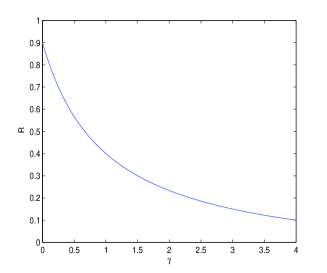
Figure 1: Convergence rate $R$ versus growth constant $\gamma$ with $p=20$, $\varepsilon=1/p$ and $r=2$

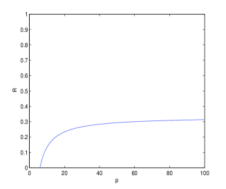
Figure 2: Convergence rate $R$ versus $p$ with $\gamma=2$, $\varepsilon=1/p$ and $r=2$

3.2 Convergence and convergence rate of the truncated EM method in $\mathcal{L}^{r}(0<r<2)$

In this subsection, we will discuss the convergence in $\mathcal{L}^{r}(0<r<2)$ under the assumption that the drift, diffusion and jump terms behave like a polynomial. For this purpose, we first impose the following assumptions.

Assumption 3.15

There exists positive constant $K_{n}$ such that

$$\left|{f(x)-f(y)}\right|\vee{\left|{g(x)-g(y)}\right|}\vee{\left|{h(x)-h(y)}\right|}\leq K_{n}{|{x-y}|},\quad\forall x,y\in\mathbb{R}^{d},\;|x|\vee|y|\leq n.$$ (3.58)

Assumption 3.16

There exist constants $\bar{K}>0$ such that

$$2x^{T}f(x)+|g(x)|^{2}+\lambda(2x^{T}h(x)+|h(x)|^{2})\leq\bar{K}(1+|x|^{2}),\quad\forall x\in\mathbb{R}^{d}.$$ (3.59)

We also give a known result as a lemma.

Lemma 3.17

Under Assumption 3.15 and 3.16 the SDE (2.1) has a unique global solution $x(t)$, moreover,

$$\sup_{0\leq t\leq T}\mathbb{E}|x(t)|^{2}<\infty,\quad\forall T>0.$$ (3.60)

In this subsection, all the three coefficients of the SDEs are allowed to grow super-linearly. Hence, we have to truncate the three terms. Similarly, we first choose a strictly increasing function $\mu:\mathbb{R}^{+}\rightarrow\mathbb{R}^{+}$ such that $\mu(n)\rightarrow\infty$, as $n\rightarrow\infty$, and

$$\sup_{|x|\leq n}|f(x)|\vee|g(x)|\vee|h(x)|\leq\mu(n),\quad\forall n\geq 1.$$ (3.61)

Denoted by $\mu^{-1}$ is the inverse function of $\mu$. We also choose a constant $\Delta^{\ast}\in(0,1)$ and a strictly decreasing function $\varphi:(0,\Delta^{\ast})\rightarrow(0,\infty)$ such that

$$\varphi(\Delta^{\ast})\geq\mu(1),\quad\lim_{\Delta\to 0}\varphi(\Delta)=\infty\quad\textrm{ and}\quad\varphi(\Delta)\Delta^{1/4}\leq 1.$$ (3.62)

For a given step size $\Delta\in(0,\Delta^{\ast})$, the truncated functions are defined as below

$$f_{\Delta}(x)=f(\pi_{\Delta}(x)),\quad g_{\Delta}(x)=g(\pi_{\Delta}(x))\quad\textrm{and}\quad h_{\Delta}(x)=h(\pi_{\Delta}(x)),\quad\forall x\in\mathbb{R}^{d},$$

where $\pi_{\Delta}$ is defined as the same as before. The following lemma also shows that the truncated functions preserve the Khaminskii-type condition. The proof is given in the Appendix.

Lemma 3.18

Let Assumption 3.16 hold. Then, for all $\Delta\in(0,\Delta^{\ast}]$, we have

$$2x^{T}f_{\Delta}(x)+|g_{\Delta}(x)|^{2}+\lambda(2x^{T}h_{\Delta}(x)+|h_{\Delta}(x)|^{2})\leq 2\bar{K}(1+|x|^{2}),\quad\forall x\in\mathbb{R}^{d}.$$ (3.63)

We now give the discrete-time truncated EM scheme

$$X_{\Delta}(t_{k+1}^{-})=X_{\Delta}(t_{k}^{-})+f_{\Delta}(X_{\Delta}(t_{k}^{-}))\Delta+g_{\Delta}(X_{\Delta}(t_{k}^{-}))\Delta B_{k}+h_{\Delta}(X_{\Delta}(t_{k}^{-}))\Delta N_{k},\quad 0\leq k\leq M-1,$$ (3.64)

where $X_{\Delta}(t_{k}^{-})$, $\Delta B_{k}$ and $\Delta N_{k}$ is defined the same as before. The continuous-time form is defined by

$$x_{\Delta}(t^{-})=x_{0}+\int_{0}^{t}f_{\Delta}(\bar{x}_{\Delta}(s^{-}))ds+\int_{0}^{t}g_{\Delta}(\bar{x}_{\Delta}(s^{-}))dB(s)+\int_{0}^{t}h_{\Delta}(\bar{x}_{\Delta}(s^{-}))dN(s).$$ (3.65)

where $\bar{x}_{\Delta}(t^{-})$ is defined in (3.12). In order to state our main result, we first give some useful lemmas.

Lemma 3.19

For any $\Delta\in(0,\Delta^{\ast})$ and $t>0$, we have

$$\mathbb{E}|x_{\Delta}(t^{-})-\bar{x}_{\Delta}(t^{-})|^{\hat{p}} \leq C_{\hat{p}}(\varphi(\Delta))^{\hat{p}}\Delta,\quad{\hat{p}}\geq 2,$$ (3.66)

$$\mathbb{E}|x_{\Delta}(t^{-})-\bar{x}_{\Delta}(t^{-})|^{\hat{p}} \leq C_{\hat{p}}(\varphi(\Delta))^{\hat{p}}\Delta^{\hat{p}/2},\quad 0<{\hat{p}}<2.$$ (3.67)

Consequently,

$$\lim_{\Delta\to 0}\mathbb{E}|x_{\Delta}(t^{-})-\bar{x}_{\Delta}(t^{-})|^{\hat{p}}=0,\quad\forall t\geq 0.$$ (3.68)

Proof. Fix any $\Delta\in(0,\Delta^{\ast}]$, $t\geq 0$ and $\hat{p}\geq 2$. There is an integer $k\geq 0$ such that $t_{k}^{-}\leq t<t_{k+1}^{-}$. By Assumption , we have

$$\mathbb{E}|x_{\Delta}(t^{-})-\bar{x}_{\Delta}(t^{-})|^{\hat{p}}$$ (3.69)

$$\leq C_{\hat{p}}\left(\mathbb{E}\left|\int_{t_{k}^{-}}^{t}f_{\Delta}(\bar{x}_{\Delta}(s^{-}))ds\right|^{\hat{p}}+\mathbb{E}\left|\int_{t_{k}^{-}}^{t}g_{\Delta}(\bar{x}_{\Delta}(s^{-}))dB(s)\right|^{\hat{p}}+\mathbb{E}\left|\int_{t_{k}^{-}}^{t}h_{\Delta}(\bar{x}_{\Delta}(s^{-}))dN(s)\right|^{\hat{p}}\right)$$

$$\leq C_{\hat{p}}\Big{(}\Delta^{\hat{p}-1}\mathbb{E}\int_{t_{k}^{-}}^{t}\left|f_{\Delta}(\bar{x}_{\Delta}(s^{-}))\right|^{\hat{p}}ds+\Delta^{(\hat{p}-2)/2}\mathbb{E}\int_{t_{k}^{-}}^{t}\left|g_{\Delta}(\bar{x}_{\Delta}(s^{-}))\right|^{\hat{p}}ds+\mathbb{E}\left|\int_{t_{k}^{-}}^{t}h_{\Delta}(\bar{x}_{\Delta}(s^{-}))dN(s)\right|^{\hat{p}}\Big{)}$$

$$\leq C_{\hat{p}}\Big{(}\Delta^{p/2}(\varphi(\Delta))^{\hat{p}}+\mathbb{E}\left|\int_{t_{k}^{-}}^{t}h_{\Delta}(\bar{x}_{\Delta}(s^{-}))dN(s)\right|^{\hat{p}}\Big{)},$$

where $C_{{\hat{p}}}$ is a generic constant. The property of Poisson increments implies

$$\mathbb{E}\left|\int_{t_{k}^{-}}^{t}h_{\Delta}(\bar{x}_{\Delta}(s^{-}))dN(s)\right|^{\hat{p}} \leq(\varphi(\Delta))^{\hat{p}}\mathbb{E}|\Delta N_{k}|^{\hat{p}}$$

$$\leq c_{0}(\varphi(\Delta))^{\hat{p}}\Delta.$$

Inserting this into (3.69) and recalling $\hat{p}\geq 2$ gives

$$\mathbb{E}|x_{\Delta}(t^{-})-\bar{x}_{\Delta}(t^{-})|^{\hat{p}}\leq C_{\hat{p}}(\varphi(\Delta))^{\hat{p}}\Delta.$$

Noting from (3.8) that $(\varphi(\Delta))^{\hat{p}}\Delta=(\varphi(\Delta))^{\hat{p}}\Delta^{1/2}\Delta^{1/2}\leq\Delta^{1/2}$, we obtain (3.68) form (3.66).
For $0<\hat{p}<2$, we have

$$\mathbb{E}|x_{\Delta}(t^{-})-\bar{x}_{\Delta}(t^{-})|^{\hat{p}}\leq\Big{(}\mathbb{E}|x_{\Delta}(t^{-})-\bar{x}_{\Delta}(t^{-})|^{2}\Big{)}^{\hat{p}/2}$$

$$\leq\Big{(}C_{\hat{p}}(\varphi(\Delta))^{2}\Delta\Big{)}^{\hat{p}/2}=C_{\hat{p}}(\varphi(\Delta))^{\hat{p}}\Delta^{\hat{p}/2}.$$

Thus, the proof is complete. $\Box$

The following lemma give the moment bound of the truncated EM solutions.

Lemma 3.20

Let Assumption 3.15 and 3.16 hold. Then

$$\sup_{0\leq\Delta\leq\Delta^{\ast}}\sup_{0\leq t\leq T}\mathbb{E}|x_{\Delta}(t^{-})|^{2}\leq C,\quad\forall T>0.$$ (3.70)

Proof. Fix any $\Delta\in(0,\Delta^{\ast})$ and $T>0$. By the Itô formula and Assumption 3.16, we have

$$\mathbb{E}|x_{\Delta}(t^{-})|^{2} \leq\mathbb{E}|x_{0}|^{2}+\mathbb{E}\int_{0}^{t}\Big{(}2x^{T}_{\Delta}(s^{-})f_{\Delta}(\bar{x}_{\Delta}(s^{-}))+|g_{\Delta}(\bar{x}_{\Delta}(s^{-}))|^{2}\Big{)}ds$$

$$\quad+\lambda\mathbb{E}\int_{0}^{t}\Big{(}2x_{\Delta}(s^{-})^{T}h_{\Delta}(\bar{x}_{\Delta}(s^{-}))+|h_{\Delta}(\bar{x}_{\Delta}(s^{-}))|^{2}\Big{)}ds$$

$$\leq\mathbb{E}|x_{0}|^{2}+\mathbb{E}\int_{0}^{t}\Big{(}2\bar{x}_{\Delta}^{T}(s^{-})f_{\Delta}(\bar{x}_{\Delta}(s^{-}))+|g_{\Delta}(\bar{x}_{\Delta}(s^{-}))|^{2}\Big{)}ds$$

$$\quad+\lambda\mathbb{E}\int_{0}^{t}\Big{(}2\bar{x}_{\Delta}^{T}(s^{-})h_{\Delta}(\bar{x}_{\Delta}(s^{-}))+|h_{\Delta}(\bar{x}_{\Delta}(s^{-}))|^{2}\Big{)}ds+\bar{J}_{1}$$

$$\leq\mathbb{E}|x_{0}|^{2}+2\bar{K}\int_{0}^{t}\Big{(}1+\mathbb{E}|\bar{x}_{\Delta}(s^{-})|^{2}\Big{)}ds+\bar{J}_{1},$$ (3.71)

where

$$\bar{J}_{1}=\mathbb{E}\int_{0}^{t}\Big{(}2(x_{\Delta}(s^{-})-\bar{x}_{\Delta}(s^{-}))^{T}f_{\Delta}(\bar{x}_{\Delta}(s^{-}))+2\lambda(x_{\Delta}(s^{-})-\bar{x}_{\Delta}(s^{-}))^{T}h_{\Delta}(\bar{x}_{\Delta}(s^{-}))\Big{)}ds.$$

By Lemma 3.19, (3.61) and 3.62, we have

$$\bar{J}_{1} \leq 2(\lambda+1)\varphi(\Delta)\int_{0}^{t}\mathbb{E}|x_{\Delta}(s^{-})-\bar{x}_{\Delta}(s^{-})|ds$$

$$\leq 2(\lambda+1)TC(\varphi(\Delta))^{2}\Delta^{1/2}\leq C.$$

Inserting this into (3.2) and using Lemma 3.19 gives

$$\mathbb{E}|x_{\Delta}(t^{-})|^{2}\leq C+2\bar{K}\int_{0}^{t}\mathbb{E}|\bar{x}_{\Delta}(s^{-})|^{2}ds.$$

Hence, we have

$$\sup_{0\leq u\leq t}\mathbb{E}|x_{\Delta}(u)|^{2}\leq C+2\bar{K}\int_{0}^{t}\sup_{0\leq u\leq s}\mathbb{E}|x_{\Delta}(u)|^{2}ds.$$

The Gronwall inequality yields

$$\sup_{0\leq u\leq T}\mathbb{E}|x_{\Delta}(u)|^{p}\leq C.$$

Thus, we complete the proof. $\Box$

As the proof is in a similar way as Lemma 3.10 and 3.11 were proved, we also have the following Lemma.

Lemma 3.21

Let Assumption 3.15 and 3.16 hold. For any real number $n>|x_{0}|$, then

$$\mathbb{P}(\tau_{n}\leq T)\leq\frac{C}{n^{2}}\quad\textrm{and}\quad\mathbb{P}(\rho_{\Delta,n}\leq T)\leq\frac{C}{n^{2}},$$ (3.72)

where $\tau_{n}$ and $\rho_{\Delta,n}$ is the same as before.

Now, let us show the convergence of the truncated EM methods for the SDEs.

Theorem 3.22

Let Assumption 3.15 and 3.16 hold. Then, for any $r\in(0,2)$

$$\lim_{\Delta\to 0}\mathbb{E}|x(T)-x_{\Delta}(T)|^{r}=0$$ (3.73)

and

$$\lim_{\Delta\to 0}\mathbb{E}|x(T)-\bar{x}_{\Delta}(T)|^{r}=0.$$ (3.74)

Proof. Let $\tau_{n}$, $\rho_{\Delta,n}$, $\theta_{\Delta,n}$ and $e_{\Delta}(t)$ be the same as before. Applying the Young inequality, we have that for any $\delta>0$,

$$\mathbb{E}|e_{\Delta}(T)|^{r} =\mathbb{E}\Big{(}|e_{\Delta}(T)|^{r}\mathbb{I}_{\{\theta_{\Delta,n}>T\}}\Big{)}+\mathbb{E}\Big{(}|e_{\Delta}(T)|^{r}\mathbb{I}_{\{\theta_{\Delta,n}\leq T\}}\Big{)}$$

$$\leq\mathbb{E}\Big{(}|e_{\Delta}(T\wedge\theta_{\Delta,n})|^{r}\Big{)}+\frac{r\delta}{2}\mathbb{E}|e_{\Delta}(T)|^{2}+\frac{2-r}{2\delta^{r/(2-r)}}\mathbb{P}(\theta_{\Delta,n}\leq T).$$ (3.75)

By Lemma 3.17 and 3.20, we have

$$\mathbb{E}|e_{\Delta}(T)|^{2}\leq 2\mathbb{E}|x(T)|^{p}+2\mathbb{E}|x_{\Delta}(T)|^{p}\leq C.$$ (3.76)

Using Lemma 3.21, we obtain

$$\mathbb{P}(\theta_{\Delta,n}\leq T)\leq\mathbb{P}(\tau_{n}\leq T)+\mathbb{P}(\rho_{\Delta,n}\leq T)\leq\frac{C}{n^{2}}.$$ (3.77)

Inserting (3.76) and (3.77) into (3.2), we get

$$\mathbb{E}|e_{\Delta}(T)|^{r}\leq\mathbb{E}|e_{\Delta}(T\wedge\theta_{\Delta,n})|^{r}+\frac{Cr\delta}{2}+\frac{C(2-r)}{2n^{2}\delta^{r/(2-r)}}.$$

Now, let $\varepsilon>0$ be arbitrary. We can choose $\delta$ sufficiently small such that

$$\frac{Cr\delta}{2}\leq\frac{\varepsilon}{3}$$

and then choose $n$ sufficiently large such than

$$\frac{C(2-r)}{2n^{2}\delta^{r/(2-r)}}\leq\frac{\varepsilon}{3}.$$

We may assume that $\Delta^{\ast}$ is sufficiently small for $\mu^{-1}(\varphi(\Delta^{\ast}))\geq n$. In the same way as Theorem 3.5 in [13] was proved, we can show that for all $\Delta\in(0,\Delta^{\ast}]$

$$\mathbb{E}|e_{\Delta}(T)|^{2}\leq C\Delta,$$

which implies

$$\mathbb{E}\Big{(}|e_{\Delta}(T\wedge\theta_{\Delta,n})|^{r}\Big{)}\leq\frac{\varepsilon}{3}.$$

Hence, we obtain the required assertion (3.73). Combining this with Lemma (3.19) gives (3.74). Thus, the proof is complete. $\Box$

For the purpose of getting the convergence rates a time T, we need some additional conditions.

Assumption 3.23

There exists a constant $\bar{L}_{1}>0$ such that

$$2(x-y)^{T}(f(x)-f(y))+|g(x)-g(y)|^{2}$$

$$+2\lambda(x-y)^{T}(h(x)-h(y))+\lambda|h(x)-h(y)|^{2}\leq\bar{L}_{1}|x-y|^{2},$$ (3.78)

for any $x,y\in\mathbb{R}^{d}$.

Assumption 3.24

There exist constant $\bar{L}_{2}>0$ and $\bar{\gamma}\geq 0$ such that

$$|f(x)-f(y)|\vee|h(x)-h(y)|\leq\bar{L}_{2}(1+|x|^{\bar{\gamma}}+|y|^{\bar{\gamma}})|x-y|,\quad\forall x,y\in\mathbb{R}^{d}.$$ (3.79)

Obviously, this condition implies

$$|f(x)|\vee|h(x)|\leq\bar{L}_{3}|x|^{1+\bar{\gamma}},$$ (3.80)

where $\bar{L}_{3}=2\bar{L}_{1}+|f(0)|+|g(0)|$.

Lemma 3.25

Let Assumption 3.15, 3.16, 3.23 and 3.24 hold. Let $n>|x_{0}|$ be a real number and let $\Delta\in(0,\Delta^{\ast})$ be sufficiently small such $\mu^{-1}(\varphi(\Delta))\geq n$. Let $\tau_{n}$ and $\rho_{\Delta,n}$ be the same as before. Let

$$\theta_{\Delta,n}=\tau_{n}\wedge\rho_{\Delta,n}\quad\textrm{and }\quad e_{\Delta}(s^{-})=x(t^{-})-x_{\Delta}(t^{-})\quad\forall t>0.$$

Then

$$\mathbb{E}|e_{\Delta}(T\wedge\theta_{\Delta,n})|^{2}\leq C(\varphi(\Delta))^{2}\Delta.$$

Proof. We write $\theta_{\Delta,n}=\theta$ for simplicity. By the Itô formula and Assumption 3.23, we get that for $0\leq t\leq T$,

$$\mathbb{E}|e_{\Delta}(t\wedge\theta)|^{2}$$

$$\leq\mathbb{E}\int_{0}^{t\wedge\theta}\Big{(}2e^{T}_{\Delta}(s^{-})(f(x(s^{-}))-f_{\Delta}(\bar{x}_{\Delta}(s^{-})))+|g(x(s^{-}))-g_{\Delta}(\bar{x}_{\Delta}(s^{-}))|^{2}\Big{)}ds$$

$$\quad+\lambda\mathbb{E}\int_{0}^{t\wedge\theta}\Big{(}|e_{\Delta}(s^{-})+(h(x(s^{-}))-h_{\Delta}(\bar{x}_{\Delta}(s^{-})))|^{2}-|e_{\Delta}(s^{-})|^{2}\Big{)}ds$$

$$\leq\mathbb{E}\int_{0}^{t\wedge\theta}\Big{(}2(x(s^{-})-\bar{x}_{\Delta}(s^{-}))^{T}(f(x(s^{-}))-f_{\Delta}(\bar{x}_{\Delta}(s^{-})))+|g(x(s^{-}))-g_{\Delta}(\bar{x}_{\Delta}(s^{-}))|^{2}\Big{)}ds+\bar{J}_{2}$$

$$\quad+\mathbb{E}\int_{0}^{t\wedge\theta}\Big{(}2\lambda(x(s^{-})-\bar{x}_{\Delta}(s^{-}))^{T}(h(x(s^{-}))-h_{\Delta}(\bar{x}_{\Delta}(s^{-})))+\lambda|h(x(s^{-}))-h_{\Delta}(\bar{x}_{\Delta}(s^{-}))|^{2}\Big{)}ds+\bar{J}_{3}$$

$$\leq\bar{L}_{1}\int_{0}^{t}\mathbb{E}|x(s\wedge\theta)-\bar{x}_{\Delta}(s\wedge\theta)|^{2}ds+\bar{J}_{2}+\bar{J}_{3},$$ (3.81)

where

$$\bar{J}_{2}=2\mathbb{E}\int_{0}^{t\wedge\theta}(x_{\Delta}(s^{-})-\bar{x}_{\Delta}(s^{-}))^{T}(f(x(s^{-}))-f_{\Delta}(\bar{x}_{\Delta}(s^{-})))ds,$$

$$\bar{J}_{3}=2\lambda\mathbb{E}\int_{0}^{t\wedge\theta}(x_{\Delta}(s^{-})-\bar{x}_{\Delta}(s^{-}))^{T}(h(x(s^{-}))-h_{\Delta}(\bar{x}_{\Delta}(s^{-})))ds.$$

By the condition $\mu^{-1}(\varphi(\Delta))\geq n$ and the definition of the truncated functions $f_{\Delta}$ and $g_{\Delta}$, we have that

$$f_{\Delta}(\bar{x}_{\Delta}(s^{-}))=f(\bar{x}_{\Delta}(s^{-}))\quad\textrm{and}\quad g_{\Delta}(\bar{x}_{\Delta}(s^{-}))=g(\bar{x}_{\Delta}(s^{-})),\;\textrm{for}\;0\leq s\leq t\wedge\theta.$$

Hence, by Assumption 3.24 and the Hölder inequality as well as Lemma 3.19 and 3.20, we get that

$$\bar{J}_{2} \leq 2\mathbb{E}\int_{0}^{t\wedge\theta}|x_{\Delta}(s^{-})-\bar{x}_{\Delta}(s^{-})||f(x(s^{-}))-f(\bar{x}_{\Delta}(s^{-}))|ds$$

$$\leq 2\bar{L}_{2}\mathbb{E}\int_{0}^{t\wedge\theta}|x_{\Delta}(s^{-})-\bar{x}_{\Delta}(s^{-})||1+|x(s^{-})|^{\bar{\gamma}}+|\bar{x}_{\Delta}(s^{-})|^{\bar{\gamma}}||x(s)-\bar{x}_{\Delta}(s^{-})|ds$$

$$\leq\bar{L}_{2}\int_{0}^{t\wedge\theta}\mathbb{E}|x(s^{-})-\bar{x}_{\Delta}(s^{-})|^{2}ds+C\int_{0}^{t\wedge\theta}\mathbb{E}(1+|x(s^{-})|^{2\bar{\gamma}}+|\bar{x}_{\Delta}(s^{-})|^{2\bar{\gamma}})|x_{\Delta}(s^{-})-\bar{x}_{\Delta}(s^{-})|^{2}ds$$

$$\leq\bar{L}_{2}\int_{0}^{t}\mathbb{E}|x(s\wedge\theta)-\bar{x}_{\Delta}(s\wedge\theta)|^{2}ds$$

$$+C\int_{0}^{T}\Big{(}1+\mathbb{E}|x(s^{-})|^{2}+\mathbb{E}|\bar{x}_{\Delta}(s^{-})|^{2}\Big{)}^{\bar{\gamma}}\Big{(}\mathbb{E}|x_{\Delta}(s^{-})-\bar{x}_{\Delta}(s^{-})|^{2/(1-\bar{\gamma})}\Big{)}^{1-\bar{\gamma}}ds$$

$$\leq\bar{L}_{2}\int_{0}^{t}\mathbb{E}|x(s\wedge\theta)-\bar{x}_{\Delta}(s\wedge\theta)|^{2}ds+C(\varphi(\Delta))^{2}\Delta.$$ (3.82)

Similarly, we have

$$\bar{J}_{3} \leq\lambda\bar{L}_{2}\int_{0}^{t}\mathbb{E}|x(s\wedge\theta)-\bar{x}_{\Delta}(s\wedge\theta)|^{2}ds+C(\varphi(\Delta))^{2}\Delta.$$ (3.83)

Inserting (3.2), (3.83) into (3.2) and combining Lemma 3.19, we have

$$\mathbb{E}|e_{\Delta}(t\wedge\theta)|^{2}\leq C\int_{0}^{t}\mathbb{E}|e_{\Delta}(s\wedge\theta)|^{2}ds+C(\varphi(\Delta))^{2}\Delta.$$

The Gronwall inequality complete the proof. $\Box$

Theorem 3.26

Let Assumption 3.15, 3.16, 3.23 and 3.24 hold. Let $r\in(0,2)$. If

$$\varphi(\Delta)\geq\mu\Big{(}\bar{L}_{3}^{-(1+\bar{\gamma})}((\varphi(\Delta))^{r}\Delta^{r/2})^{-1/{(2-r)}}\Big{)}$$ (3.84)

holds for all sufficiently small $\Delta\in(0,\Delta^{\ast})$, then for every such small $\Delta$,

$$\mathbb{E}|x(T)-x_{\Delta}(T)|^{r}\leq C(\varphi(\Delta))^{r}\Delta^{r/2}$$ (3.85)

and

$$\mathbb{E}|x(T)-\bar{x}_{\Delta}(T)|^{r}\leq C(\varphi(\Delta))^{r}\Delta^{r/2}.$$ (3.86)

Proof. Let $\tau_{n}$, $\rho_{\Delta,n}$, $\theta_{\Delta,n}$ and $e_{\Delta}(t)$ be the same as before. By (3.2) - (3.77), inequality

$$\mathbb{E}|e_{\Delta}(T)|^{r}\leq\mathbb{E}|e_{\Delta}(T\wedge\theta_{\Delta,n})|^{r}+\frac{Cr\delta}{2}+\frac{C(2-r)}{2n^{2}\delta^{r/(2-r)}}$$

holds for any $\Delta\in(0,\Delta^{\ast})$, $n>|x_{0}|$ and $\delta>0$. We can therefore choose $\delta=(\varphi(\Delta))^{r}\Delta^{r/2}$ and $n=\bar{L}_{3}^{-(1+\bar{\gamma})}((\varphi(\Delta))^{r}\Delta^{r/2})^{-1/{(2-r)}}$ to get

$$\mathbb{E}|e_{\Delta}(T)|^{r}\leq\mathbb{E}|e_{\Delta}(T\wedge\theta_{\Delta,n})|^{r}+C(\varphi(\Delta))^{r}\Delta^{r/2}.$$

By condition (3.84), we have

$$\mu^{-1}(\varphi(\Delta))\geq\bar{L}_{4}^{-{1+\bar{\gamma}}}((\varphi(\Delta))^{r}\Delta^{r/2})^{-1/{(2-r)}}=n.$$

Using Lemma 3.25, we have

$$\mathbb{E}|e_{\Delta}(T)|^{r}\leq(\mathbb{E}|e_{\Delta}(T)|^{2})^{r/2}\leq C((\varphi(\Delta))^{2}\Delta)^{r/2}=C(\varphi(\Delta))^{r}\Delta^{r/2}.$$

Combining this with Lemma (3.19) gives (3.86). Thus, the proof is complete. $\Box$

Corollary 3.27

Let Assumption 3.15, 3.16, 3.23 and 3.24 hold. Define

$$\mu(n)=\bar{L}_{3}n^{1+\bar{\gamma}},\quad n\geq 0.$$ (3.87)

Let $0<r\leq 2/(2+\bar{\gamma})$ and

$$\varphi(\Delta)=\Delta^{-\varepsilon},\quad\varepsilon\in\Big{[}\frac{r(1+\bar{\gamma})}{4+2r\bar{\gamma}},\frac{1}{4}\Big{]}.$$ (3.88)

Assume that $\bar{\Delta}\in(0,1)$ and

$$\varphi(\bar{\Delta})\geq\mu\Big{(}\bar{L}_{3}^{-(1+\bar{\gamma})}({\bar{\Delta}}^{r/2}(\varphi({\bar{\Delta}}))^{r})^{-1/{(2-r)}}\Big{)}$$ (3.89)

hold. Then, for every $\Delta\in(0,\bar{\Delta})$ ,

$$\mathbb{E}|x(T)-x_{\Delta}(T)|^{r}\leq C\Delta^{r/2-r\varepsilon}$$ (3.90)

and

$$\mathbb{E}|x(T)-\bar{x}_{\Delta}(T)|^{r}\leq C\Delta^{r/2-r\varepsilon}.$$ (3.91)

Proof. Applying Theorem 3.26 along with (3.87) and (3.88) gives the required assertion (3.90) and (3.91). $\Box$

Remark 3.28

Substituting (3.87) and (3.88) into (3.89) gives

$$\bar{\Delta}^{-\varepsilon}\geq\bar{\Delta}^{-r(1-2\varepsilon)(1+\bar{\gamma})/(2(2-r))},\quad\textrm{namely}\quad\varepsilon\geq\frac{r(1+\bar{\gamma})}{4+2r\bar{\gamma}}.$$

But, condition (3.88) means

$$\frac{r(1+\bar{\gamma})}{4+2r\bar{\gamma}}\leq\frac{1}{4},\quad\textrm{namely}\quad r\leq\frac{2}{2+\bar{\gamma}}\leq 1.$$

Hence, we have to force $r$ to be not greater than $2/(2+\bar{\gamma})$ in the corollary 3.27.

Remark 3.29

Fixing $\bar{\gamma}\geq 0$, by (3.88) and (3.90), we can conclude that convergence rate is a increasing function with respect to $\varepsilon$. Hence, substituting

$$\varepsilon=\frac{r(1+\bar{\gamma})}{4+2r\bar{\gamma}}$$

into $r/2(1-2\varepsilon)$ obtains the optimal $\mathcal{L}^{r}$-convergence rate, that is

$$R:=\frac{r(2-r)}{2(2+r\bar{\gamma})},\quad\textrm{ for}\quad 0<r\leq\frac{2}{2+\bar{\gamma}},$$ (3.92)

which means convergence rate $R$ increases as $r$ increases. In other words, the higher moment has a better convergence rate for SDEs with jumps when $0<r\leq 2/(2+\bar{\gamma})$. If we take

$$r=\frac{2}{2+\bar{\gamma}},$$

then (3.92) becomes

$$R=\frac{1}{4+2\bar{\gamma}},$$

this is the maximum of optimal $\mathcal{L}^{r}$-convergence rate. In particular, if $\bar{\gamma}=0$, i.e. the drift and diffusion coefficients grows linearly, then convergence rate is equal to $1/4$ by choosing $r=1$.

4 Asymptotic behaviours

4.1 Stability

In this subsection, we will show that the partially truncated EM method can preserve the mean square exponential stability of the underlying SDEs (2.1). For the purpose of stability, we also assume that

$$f(0)=g(0)=h(0)=0,$$ (4.1)

which means

$$|F_{1}(x)|\vee|G_{1}(x)|\vee|h(x)|\leq K_{1}|x|,\quad\forall x\in\mathbb{R}^{d}.$$ (4.2)

We first impose the following assumption.

Assumption 4.1

Assume that there exist positive constant $\alpha_{1}\geq\alpha_{2}+\lambda K_{1}(2+K_{1})$ and $\theta\in(0,\infty)$ such that

$$2x^{T}F_{1}(x)+(1+\theta)|G_{1}(x)|^{2}\leq-\alpha_{1}|x|^{2}$$

and

$$2x^{T}F(x)+(1+\theta^{-1})|G(x)|^{2}\leq\alpha_{2}|x|^{2}$$

for all $x\in\mathbb{R}^{d}$.

If there is no super-linear term $G(x)$, we set $\theta=0$ and $\theta^{-1}|G(x)|^{2}=0$. Similarly, when linear term $G_{1}(x)$ is absent, we set $\theta=\infty$ and $\theta|G_{1}(x)|^{2}=0$. Moreover, this assumption means

$$2x^{T}f(x)+|g(x)|^{2}+\lambda(x^{T}h(x)+|h(x)|^{2})\leq-(\alpha_{1}-\alpha_{2}-\lambda K_{1}(2+K_{1}))|x|^{2},\quad x\in\mathbb{R}^{d}.$$ (4.3)

It is therefore known that the SDEs (2.1) is exponentially stable in the mean square sense. We state the following Lemma.

Lemma 4.2

Let Assumption 3.1 - 3.3 and 4.1 hold. Then for any initial value $x_{0}\in\mathbb{R}^{d}$, the solution of the SDEs (2.1) satisfies

$$\mathbb{E}|x(t)|^{2}\leq|x_{0}|^{2}e^{-(\alpha_{1}-\alpha_{2}-\lambda K_{1}(2+K_{1}))t^{-}},\quad\forall t\geq 0.$$

The following theorem shows that the truncated EM method preserves this mean square exponential stability perfectly. We will employ the technique due to Guo et al. [23] to prove our results.

Theorem 4.3

Let Assumption 3.1, 3.2, 3.3 and 4.1 hold. Then for any $\epsilon\in(0,\alpha_{1}-\alpha_{2}-\lambda K_{1}(2+K_{1}))$, there exists a $\hat{\Delta}\in(0,\Delta^{\ast})$ such that for all $\Delta\in(0,\hat{\Delta})$ and any initial value $x_{0}\in\mathbb{R}^{d}$, the solution of the truncated EM method (3.11) satisfies

$$\mathbb{E}|X_{\Delta}(t_{k}^{-})|^{2}\leq|x_{0}|^{2}e^{-(\alpha_{1}-\alpha_{2}-\lambda K_{1}(2+K_{1})-\epsilon)t_{k}^{-}},\quad\forall k\geq 0.$$ (4.4)

Proof. Fix $\Delta\in(0,\Delta^{\ast})$. In the same way as Theorem 4.3 in [23] was proved, we have

$$2x^{T}f_{\Delta}(x)+|g_{\Delta}(x)|^{2}\leq-(\alpha_{1}-\alpha_{2})|x|^{2},\quad\forall x\in\mathbb{R}^{d}.$$ (4.5)

From (3.11), we have

$$\mathbb{E}|X_{\Delta}(t_{k+1}^{-})|^{2} =\mathbb{E}\Big{(}|X_{\Delta}(t_{k}^{-})|^{2}+|f_{\Delta}(X_{\Delta}(t_{k}^{-}))|^{2}\Delta^{2}+|g_{\Delta}(X_{\Delta}(t_{k}^{-}))\Delta B_{k}|^{2}$$

$$\quad+2X_{\Delta}(t_{k}^{-})^{T}f_{\Delta}(X_{\Delta}(t_{k}^{-}))\Delta+|h(X_{\Delta}(t_{k}^{-}))\Delta N_{k}|^{2}$$

$$\quad+2\Delta f_{\Delta}^{T}(X_{\Delta}(t_{k}^{-}))h(X_{\Delta}(t_{k}^{-}))\Delta N_{k}+2X_{\Delta}(t_{k}^{-})^{T}h(X_{\Delta}(t_{k}^{-}))\Delta N_{k}\Big{)}$$ (4.6)

for $0\leq k\leq M-1.$ The property of Brownian increments implies

$$\mathbb{E}|g_{\Delta}(X_{\Delta}(t_{k}^{-}))\Delta B_{k}|^{2}=\Delta\mathbb{E}|g_{\Delta}(X_{\Delta}(t_{k}^{-}))|^{2}.$$

But, the Poisson increments satisfy $\mathbb{E}\Delta N_{k}=\lambda\Delta$ and $\mathbb{E}(\Delta N_{k})^{2}=\lambda\Delta(1+\lambda\Delta)$. Hence, using the independence of the increments and (4.2), we find that

$$2\mathbb{E}|X_{\Delta}(t_{k}^{-})h(X_{\Delta}(t_{k}^{-}))\Delta N_{k}|\leq 2K_{1}\mathbb{E}|X_{\Delta}(t_{k}^{-})|^{2}\mathbb{E}|\Delta N_{k}|=2K_{1}\lambda\Delta\mathbb{E}|X_{\Delta}(t_{k}^{-})|^{2},$$ (4.7)

$$\mathbb{E}|h(X_{\Delta}(t_{k}^{-}))\Delta N_{k}|^{2} \leq K_{1}^{2}\mathbb{E}|X_{\Delta}(t_{k}^{-})|^{2}\mathbb{E}|\Delta N_{k}|^{2}$$

$$\leq K_{1}^{2}\lambda\Delta(1+\lambda\Delta)\mathbb{E}|X_{\Delta}(t_{k}^{-})|^{2}$$

$$=K_{1}^{2}\lambda\Delta\mathbb{E}|X_{\Delta}(t_{k}^{-})|^{2}+K_{1}^{2}\lambda^{2}\Delta^{2}\mathbb{E}|X_{\Delta}(t_{k}^{-})|^{2}$$ (4.8)

and

$$2\mathbb{E}|\Delta f_{\Delta}(X_{\Delta}(t_{k}^{-}))h(X_{\Delta}(t_{k}^{-}))\Delta N_{k}| \leq 2K_{1}\Delta\mathbb{E}(|X_{\Delta}(t_{k}^{-})f_{\Delta}(X_{\Delta}(t_{k}^{-}))|)\mathbb{E}|\Delta N_{k}|$$

$$\leq K_{1}\lambda\Delta^{2}(\mathbb{E}|X_{\Delta}(t_{k}^{-})|^{2}+\mathbb{E}|f_{\Delta}(X_{\Delta}(t_{k}^{-}))|^{2}).$$ (4.9)

Substituting (4.7)-(4.1) into (4.1) gives

$$\mathbb{E}|X_{\Delta}(t_{k+1}^{-})|^{2} \leq\mathbb{E}\Big{(}|X_{\Delta}(t_{k}^{-})|^{2}+2X_{\Delta}(t_{k}^{-})^{T}f_{\Delta}(X_{\Delta}(t_{k}^{-}))\Delta+|g_{\Delta}(X_{\Delta}(t_{k}^{-}))|^{2}\Delta\Big{)}$$

$$\quad+\lambda K_{1}(2+K_{1})\Delta\mathbb{E}|X_{\Delta}(t_{k}^{-})|^{2}+(1+K_{1}\lambda)\Delta^{2}\mathbb{E}|f_{\Delta}(X_{\Delta}(t_{k}^{-}))|^{2}$$

$$\quad+(K_{1}^{2}\lambda^{2}+K_{1}\lambda)\Delta^{2}\mathbb{E}|X_{\Delta}(t_{k}^{-})|^{2}.$$ (4.10)

By (4.5), we have

$$\mathbb{E}|X_{\Delta}(t_{k+1}^{-})|^{2} \leq(1-(\alpha_{1}-\alpha_{2}-\lambda K_{1}(2+K_{1}))\Delta)\mathbb{E}|X_{\Delta}(t_{k}^{-})|^{2}$$

$$\quad+(1+K_{1}\lambda)\Delta^{2}\mathbb{E}|f_{\Delta}(X_{\Delta}(t_{k}^{-}))|^{2}+(K_{1}^{2}\lambda^{2}+K_{1}\lambda)\Delta^{2}\mathbb{E}|X_{\Delta}(t_{k}^{-})|^{2}.$$ (4.11)

By (3.1) and (4.1), we have

$$|F_{\Delta}(x)|^{2}\leq 4L_{1}|x|^{2},\;\textrm{if}\;|x|\leq 1,$$

and

$$|F_{\Delta}(x)|^{2}\leq(\varphi(\Delta))^{2}\leq(\varphi(\Delta))^{2}|x|^{2},\;\textrm{if}\;|x|>1.$$

Hence, we have

$$\Delta|f_{\Delta}(x)|^{2} \leq 2(K_{1}^{2}+4L_{1}+(\varphi(\Delta))^{2})\Delta|x|^{2}$$

$$\leq 2\Big{(}(K_{1}^{2}+4L_{1})\Delta+\Delta^{1/2\wedge(\bar{p}-2)/\bar{p}}\Big{)}|x|^{2}$$

for all $x\in\mathbb{R}^{d}$, where (3.8) have been used. For any $\epsilon\in(0,\alpha_{1}-\alpha_{2}-\lambda K_{1}(2+K_{1}))$, there is a $\hat{\Delta}\in(0,\Delta^{\ast})$ sufficiently small such that for all $\Delta\in(0,\hat{\Delta})$, $(\alpha_{1}-\alpha_{2}-\lambda K_{1}(2+K_{1}))\Delta\leq 1$ and

$$\begin{cases}2(1+K_{1}\lambda)\Big{(}(K_{1}^{2}+4L_{1})\Delta+\Delta^{1/2\wedge(\bar{p}-2)/\bar{p}}\Big{)}\leq 0.5\epsilon\\ (K_{1}^{2}\lambda^{2}+K_{1}\lambda)\Delta\leq 0.5\epsilon.\end{cases}$$ (4.12)

For each such $\Delta$, we have

$$(1+K_{1}\lambda)\Delta^{2}\mathbb{E}|f_{\Delta}(X_{\Delta}(t_{k}^{-}))|^{2}+(K_{1}^{2}\lambda^{2}+K_{1}\lambda)\Delta^{2}\mathbb{E}|X_{\Delta}(t_{k}^{-})|^{2}\leq\epsilon\Delta\mathbb{E}|X_{\Delta}(t_{k}^{-})|^{2}.$$

Inserting this into (4.1), we yield

$$\mathbb{E}|X_{\Delta}(t_{k+1}^{-})|^{2} \leq(1-(\alpha_{1}-\alpha_{2}-\lambda K_{1}(2+K_{1})-\epsilon))\Delta)\mathbb{E}|X_{\Delta}(t_{k}^{-})|^{2}$$

$$\leq\cdots$$

$$\leq|x_{0}|^{2}(1-(\alpha_{1}-\alpha_{2}-\lambda K_{1}(2+K_{1})-\epsilon))\Delta)^{k+1}.$$ (4.13)

Elementary inequality $1+x\leq e^{x},\;\forall x\in\mathbb{R}$ gives

$$\mathbb{E}|X_{\Delta}(t_{k+1}^{-})|^{2}\leq|x_{0}|^{2}e^{-(\alpha_{1}-\alpha_{2}-\lambda K_{1}(2+K_{1})-\epsilon)t_{k+1}^{-}}.$$ (4.14)

Thus, the proof is complete. $\Box$

4.2 Asymptotic boundedness

In this subsection, we will show that the truncated EM method maintains the asymptotic boundedness of the underlying of SDEs (2.1). The additional assumption is the following one.

Assumption 4.4

Assume that there exist constant $\bar{\alpha}_{1},\bar{\alpha}_{2},\bar{\beta}_{2}>0$ and $\bar{\beta}_{1}>\bar{\beta}_{2}+\max(\lambda(4K_{1}^{2}+1),2\lambda K_{1}(2+K_{1}))$ such that

$$2x^{T}F_{1}(x)+(1+\theta)|G_{1}(x)|^{2}\leq\bar{\alpha}_{1}-\bar{\beta}_{1}|x|^{2}$$

and

$$2x^{T}F(x)+(1+\theta^{-1})|G(x)|^{2}\leq\bar{\alpha}_{2}+\bar{\beta}_{2}|x|^{2}$$

for all $a\in\mathbb{R}^{d}$.

When there is no super-linear term $G(x)$, we set $\theta=0$ and $\theta^{-1}|G(x)|^{2}=0$. Similarly, if linear term $G_{1}(x)$ is absent, we set $\theta=\infty$ and $\theta|G_{1}(x)|^{2}=0$. Moreover, (3.2) implies

$$\lambda(2x^{T}h(x)+|h(x)|^{2})\leq\lambda(|x|^{2}+2|h(x)|^{2})\leq 4\lambda K_{1}^{2}+\lambda(4K_{1}+1)|x|^{2},\quad\forall x\in\mathbb{R}^{d}.$$

Hence, by Assumption 4.4, we have

$$2x^{T}f(x)+|g(x)|^{2}+\lambda(2x^{T}h(x)+|h(x)|^{2})\leq\hat{\alpha}-\hat{\beta}|x|^{2},\quad\forall x\in\mathbb{R}^{d},$$ (4.15)

where $\hat{\alpha}=\bar{\alpha}_{1}+\bar{\alpha}_{2}+4\lambda K_{1}^{2}$ and $\hat{\beta}=\bar{\beta}_{1}-\bar{\beta}_{2}-\lambda(4K_{1}^{2}+1)$.

Theorem 4.5

Let Assumption 3.1, 3.2, 3.3 and 4.4 hold. Then for any initial value $x_{0}\in\mathbb{R}^{d}$, the solution of the SDEs (2.1) satisfy

$$\mathop{\lim\sup}\limits_{t\to\infty}\mathbb{E}|x(t)|^{2}\leq\frac{\bar{\alpha}_{1}+\bar{\alpha}_{2}+4\lambda K_{1}^{2}}{\bar{\beta}_{1}-\bar{\beta}_{2}-\lambda(4K_{1}^{2}+1)}.$$ (4.16)

Proof. Let $\tau_{n}$ , $\hat{\alpha}$, and $\hat{\beta}$ be the same as before, $\sigma_{n}=t\wedge\tau_{n}$. For any $t\geq 0$, the Itô formula gives that

$$\mathbb{E}\Big{[}e^{\hat{\beta}\sigma_{n}}|x(\sigma_{n})|^{2}\Big{]} =|x_{0}|^{2}+\mathbb{E}\int_{0}^{\sigma_{n}}e^{\hat{\beta}\sigma_{n}}\Big{(}2x^{T}(s)f(x(s))+|g(x(s))|^{2}$$

$$+2x^{T}(s)h(x(s))+|h(x(s))|^{2}+\hat{\beta}|x(s)|^{2}\Big{)}ds.$$

By (4.15), we have

$$\mathbb{E}\Big{[}e^{\hat{\beta}\sigma_{n}}|x(\sigma_{n})|^{2}\Big{]} \leq|x_{0}|^{2}+\hat{\alpha}\int_{0}^{t}e^{\hat{\beta}s}ds=|x_{0}|^{2}+\frac{\hat{\alpha}}{\hat{\beta}}(e^{\hat{\beta}t^{-}}-1).$$

Letting $n\to\infty$, we have

$$\mathbb{E}\Big{[}e^{\hat{\alpha}t}|x(t)|^{2}\Big{]} \leq|x_{0}|^{2}+\frac{\hat{\alpha}}{\hat{\beta}}(e^{\hat{\beta}t^{-}}-1)$$

which implies

$$\mathbb{E}|x(t)|^{2}\ \leq\frac{|x_{0}|^{2}}{e^{\hat{\beta}t^{-}}}+\frac{\hat{\alpha}}{\hat{\beta}}.$$

Thus, the proof is complete. $\Box$

Lemma 4.6

Let $0<A<1$ and $B\geq 0$. If

$$D_{k}\leq AD_{k-1}+B,\quad\textrm{for}\quad k=0,1,2,\cdots.$$ (4.17)

Then

$$\mathop{\lim\sup}\limits_{k\to\infty}D_{k}\leq\frac{B}{1-A}.$$ (4.18)

Proof. The proof is given in the Appendix. $\Box$

Theorem 4.7

Let Assumption 3.1, 3.2, 3.3 and 4.4 hold. Then for any $\epsilon\in\big{(}0,\bar{\beta}_{1}-\bar{\beta}_{2}-\max(\lambda(4K_{1}^{2}+1),2\lambda K_{1}(2+K_{1}))\big{)}$, there is a $\hat{\Delta}\in(0,\Delta^{\ast})$ and any initial value $x_{0}\in\mathbb{R}^{d}$, the solution of the partially truncated EM method satisfy

$$\mathop{\lim\sup}\limits_{k\to\infty}\mathbb{E}|X_{\Delta}(t_{k}^{-})|^{2}\leq\frac{\bar{\alpha}_{1}+\bar{\alpha}_{2}+2\lambda K_{1}(2+K_{1})+\epsilon}{\bar{\beta}_{1}-\bar{\beta}_{2}-2\lambda K_{1}(2+K_{1})-\epsilon}.$$ (4.19)

Proof. Fix $\varepsilon\in(0,\bar{\beta}_{1}-\bar{\beta}_{2})$. In the same way as Theorem 5.3 in [23] was proved, we have

$$2x^{T}f_{\Delta}(x)+|g_{\Delta}(x)|^{2}\leq\bar{\alpha}_{1}+\bar{\alpha}_{2}-(\bar{\beta}_{1}-\bar{\beta}_{2}-0.5\epsilon)|x|^{2},\quad\forall x\in\mathbb{R}^{d}.$$ (4.20)

as long as $\Delta\in(0,\hat{\Delta}_{1})$, where $\hat{\Delta}_{1}\in(0,\Delta^{\ast})$ is sufficiently small for which

$$\frac{\bar{\alpha}_{2}}{(\mu^{-1}(\varphi(\hat{\Delta}_{1})))^{2}}\leq 0.5\epsilon.$$ (4.21)

Using the independence of the Poisson increments and (3.2) as well as Lemma 3.7, we obtain that

$$\mathbb{E}|h(X_{\Delta}(t_{k}^{-}))\Delta N_{k}|^{2} \leq 2K_{1}^{2}\mathbb{E}(1+|X_{\Delta}(t_{k}^{-})|^{2})\mathbb{E}|\Delta N_{k}|^{2}$$

$$\leq 2K_{1}^{2}\lambda\Delta(1+\lambda\Delta)\mathbb{E}(1+|X_{\Delta}(t_{k}^{-})|^{2})$$

$$\leq 2K_{1}^{2}\lambda\Delta\mathbb{E}|X_{\Delta}(t_{k}^{-})|^{2}+2K_{1}^{2}\lambda\Delta+C\Delta^{2},$$ (4.22)

$$2\mathbb{E}|X_{\Delta}(t_{k}^{-})h(X_{\Delta}(t_{k}^{-}))\Delta N_{k}| \leq 2K_{1}\mathbb{E}(|X_{\Delta}(t_{k}^{-})|(1+|X_{\Delta}(t_{k}^{-})|))\mathbb{E}|\Delta N_{k}|$$

$$\leq 4K_{1}\lambda\Delta\mathbb{E}(1+|X_{\Delta}(t_{k}^{-})|^{2})$$

$$\leq 4K_{1}\lambda\Delta\mathbb{E}|X_{\Delta}(t_{k}^{-})|^{2}+4K_{1}\lambda\Delta$$ (4.23)

and

$$2\mathbb{E}|\Delta f_{\Delta}(X_{\Delta}(t_{k}^{-}))h(X_{\Delta}(t_{k}^{-}))\Delta N_{k}| \leq 2K_{1}\Delta\mathbb{E}((1+|X_{\Delta}(t_{k}^{-})|)|f_{\Delta}(X_{\Delta}(t_{k}^{-}))|)\mathbb{E}|\Delta N_{k}|$$

$$\leq K_{1}\lambda\Delta^{2}(\mathbb{E}(1+|X_{\Delta}(t_{k}^{-})|^{2})+\mathbb{E}|f_{\Delta}(X_{\Delta}(t_{k}^{-}))|^{2})$$

$$\leq K_{1}\lambda\Delta^{2}\mathbb{E}|f_{\Delta}(X_{\Delta}(t_{k}^{-}))|^{2}+C\Delta^{2}.$$ (4.24)

Fix $x_{0}\in\mathbb{R}^{d}$ arbitrarily. For any $\Delta\in(0,\hat{\Delta}_{1})$, substituting (4.2)-(4.2) into (4.1) gives

$$\mathbb{E}|X_{\Delta}(t_{k+1}^{-})|^{2} \leq\mathbb{E}\Big{(}|X_{\Delta}(t_{k}^{-})|^{2}+2X_{\Delta}(t_{k}^{-})^{T}f_{\Delta}(X_{\Delta}(t_{k}^{-}))\Delta+|g_{\Delta}(X_{\Delta}(t_{k}^{-}))|^{2}\Delta\Big{)}$$

$$\quad+2\lambda K_{1}(2+K_{1})\Delta\mathbb{E}|X_{\Delta}(t_{k}^{-})|^{2}+(1+K_{1}\lambda)\Delta^{2}\mathbb{E}|f_{\Delta}(X_{\Delta}(t_{k}^{-}))|^{2}$$

$$\quad+2\lambda K_{1}(2+K_{1})\Delta+C\Delta^{2}$$

$$\leq(1-(\bar{\beta}_{1}-\bar{\beta}_{2}-2\lambda K_{1}(2+K_{1})-0.5\varepsilon)\Delta)\mathbb{E}|X_{\Delta}(t_{k}^{-})|^{2}$$

$$\quad+(\bar{\alpha}_{1}+\bar{\alpha}_{2}+2\lambda K_{1}(2+K_{1}))\Delta+C\Delta^{2}$$

$$\quad+(1+K_{1}\lambda)\Delta^{2}\mathbb{E}|f_{\Delta}(X_{\Delta}(t_{k}^{-}))|^{2},$$ (4.25)

where (4.20) have been used. By (3.2) and (3.9), we have

$$|f_{\Delta}(x)|^{2}\leq 2|F_{1}(x)|^{2}+2|F(x)|^{2}\leq 4K_{1}^{2}(1+|x|^{2})+2(\varphi(\Delta))^{2},\quad\forall x\in\mathbb{R}^{d}.$$

Hence, by (3.8), we get

$$\Delta|f_{\Delta}(x)|^{2}\leq 4K_{1}^{2}\Delta(1+|x|^{2})+2\Delta^{1/2\wedge(\bar{p}-2)/\bar{p}},\quad\forall x\in\mathbb{R}^{d}.$$

Consequently, there is a $\hat{\Delta}\in(0,\hat{\Delta}_{1})$ sufficiently small such that for any $\Delta\in(0,\hat{\Delta})$, $\Delta(\hat{\beta}_{1}-\hat{\beta}_{2}-\epsilon)<1$ and

$$C\Delta+(1+K_{1}\lambda)\Delta|f_{\Delta}(X_{\Delta}(t_{k}^{-}))|^{2}\leq\varepsilon+0.5\epsilon|X_{\Delta}(t_{k}^{-})|^{2}.$$ (4.26)

Thus, fix any $\Delta\in(0,\hat{\Delta})$. Inserting (4.26) into (4.2) yields

$$\mathbb{E}|X_{\Delta}(t_{k+1}^{-})|^{2} \leq(1-(\bar{\beta}_{1}-\bar{\beta}_{2}-2\lambda K_{1}(2+K_{1})-\epsilon)\Delta)\mathbb{E}|X_{\Delta}(t_{k}^{-})|^{2}$$

$$\quad+(\bar{\alpha}_{1}+\bar{\alpha}_{2}+2\lambda K_{1}(2+K_{1})+\epsilon)\Delta.$$ (4.27)

Applying Lemma 4.6 to (4.2) gives the required assertion (4.19). $\Box$

5 Examples

Example 5.1

Consider the following scalar SDEs with jumps

$$dx(t^{-})=-x^{5}(t^{-})dt+x^{2}(t^{-})dB(t)+x^{2}(t^{-})dN(t),$$ (5.1)

with the initial value $x(0)=1$, where $B(t)$ is a scalar Brownian motion and $N(t)$ is a scalar Poisson process with jump intensity $\lambda=0.5$. Obviously, we have

$$f(x)=-x^{5},\quad g(x)=x^{2},\quad h(x)=x^{2}.$$

It is easy to check that Assumption 3.24 is satisfied with

$$|f(x)-f(y)|\vee|h(x)-h(y)|\leq\bar{L}_{2}(1+x^{4}+y^{4})|x-y|$$ (5.2)

for a constant $\bar{L}_{2}>0$. The elementary inequality gives

$$2\lambda(x-y)(h(x)-h(y))+\lambda|h(x)-h(y)|^{2}$$

$$=(x-y)(x^{2}-y^{2})+0.5|x^{2}-y^{2}|^{2}$$

$$\leq|x+y||x-y|^{2}+0.5|x+y|^{2}|x-y|^{2}$$

$$\leq(x^{2}+y^{2}+1)|x-y|^{2}+(x^{2}+y^{2})|x-y|^{2}$$

$$=\Big{(}2(x^{2}+y^{2})+1\Big{)}|x-y|^{2}.$$ (5.3)

Also, we have

$$-(x^{3}y+xy^{3}+x^{2}y^{2})=-xy(x^{2}+y^{2})-x^{2}y^{2}\leq 0.5(x^{4}+y^{4}).$$ (5.4)

By (5.1) and (5.4), we have

$$2(x-y)(f(x)-f(y))+|g(x)-g(y)|^{2}+2\lambda(x-y)|h(x)-h(y)|+\lambda|h(x)-h(y)|^{2}$$

$$\leq(x-y)\Big{(}-(x-y)(x^{4}+x^{3}y+x^{2}y^{2}+xy^{3}+y^{4})\Big{)}+|x^{2}-y^{2}|^{2}$$

$$\quad+\Big{(}2(x^{2}+y^{2})+1\Big{)}|x-y|^{2}$$

$$\leq-0.5(x^{4}+y^{4})|x-y|^{2}+2(x^{2}+y^{2})|x-y|^{2}+\Big{(}2(x^{2}+y^{2})+1\Big{)}|x-y|^{2}$$

$$=\Big{(}-0.5(x^{4}+y^{4})+4(x^{2}+y^{2})+1\Big{)}|x-y|^{2}$$

$$\leq 17|x-y|^{2}.$$ (5.5)

Note that in the last inequality the elementary inequality

$$kab\leq\frac{1}{2}a^{2}+\frac{1}{2}k^{2}b^{2},\quad\forall a,b,k\in\mathbb{R}$$

has been used. Hence, Assumption 3.23 is satisfied. For Assumption 3.16, we have

$$2x^{T}f(x)+|g(x)|^{2}+\lambda(2x^{T}h(x)+|h(x)|^{2})$$

$$=-2x^{6}+x^{4}+0.5(2x^{3}+x^{4})$$

$$=(-x^{6}+\frac{3}{2}x^{4})+(x^{3}-x^{6})$$

$$=x^{2}\Big{(}-(x^{2}-\frac{3}{4})^{2}+\frac{9}{16}\Big{)}+(x^{3}-x^{6})$$

$$\leq\frac{9}{16}x^{2}+\frac{1}{4},$$ (5.6)

where we use the elementary inequality $ab\leq a^{2}+b^{2}/4$ in the last inequality. By (5.2), we can choose $\mu(n)=n^{5}$ such that

$$\sup_{|x|\leq n}(|f(x)|\vee|g(x)|\vee|h(x)|)=\sup_{|x|\leq n}(|x^{5}|\vee|x^{2}|\vee|x^{2}|)\leq n^{5},\quad\forall n\geq 1.$$

Letting $\bar{\gamma}=4$, $r=2/(2+\bar{\gamma})=1/3$ and $\varepsilon=1/4$. If we choose $\varphi(\Delta)=\Delta^{-\varepsilon}=\Delta^{-1/4}$, then all the conditions in (3.62) hold for all $\Delta^{\ast}\in(0,1].$ Hence, the truncating factor is defined as $\mu^{-1}(\varphi(\Delta))=\Delta^{-1/20}$ and the truncated functions are defined as

$$f_{\Delta}(x)=f((|x|\wedge\Delta^{-0.05})\frac{x}{|x|})$$

$$g_{\Delta}(x)=g((|x|\wedge\Delta^{-0.05})\frac{x}{|x|})$$

$$h_{\Delta}(x)=h((|x|\wedge\Delta^{-0.05})\frac{x}{|x|}).$$

For the given step size $\Delta$ and the time $T$, the $X_{k+1}$ is calculated by

$$X_{k+1}=X_{k}+f_{\Delta}(X_{k})\Delta+g_{\Delta}(X_{k})\Delta B_{k}+h_{\Delta}(X_{k})\Delta N_{k},\quad 0\leq k\leq T/\Delta-1,$$ (5.7)

with $X_{0}=1$. Then, by Corollary 3.27, the truncated EM scheme converges strongly with rate $r/2-r\varepsilon=1/(4+2\bar{\gamma})=1/12$ to the true solution of the SDE 5.1.

As SDEs 5.1 does not have any explicit solutions, the scheme (5.7) with step size $2^{-16}$ is treated as the solution of the SDEs 5.1 in the numerical experiment. The number of simulation is $500$. The $\mathcal{L}^{1/3}$ errors at time $T=4$ ,that is

$$\Big{(}\mathbb{E}\big{|}X(T)-x_{\Delta}(T)\big{|}^{1/3}\Big{)}^{3}\approx\Big{(}\frac{1}{500}\sum_{i=1}^{500}\big{|}[X(T)]^{i}-[x_{\Delta}(T)]^{i}\big{|}^{1/3}\Big{)}^{3},$$

with step sizes $2^{-15}$, $2^{-14}$, $2^{-13}$, $2^{-12}$ and $2^{-11}$ are displayed in Fig 3 . The numerical result shows that our numerical findings are consistent with the theoretical results obtained in this paper.

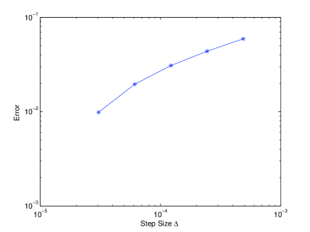
Figure 3: $\mathcal{L}^{1/3}$-convergence of truncated EM scheme 5.7 of SDEs 5.1

Example 5.2

Consider the following scalar SDEs with jumps

$$dx(t^{-})=-(x(t^{-})+x^{5}(t^{-}))dt+x^{2}(t^{-})dB(t)+x(t^{-})dN(t),$$ (5.8)

with the initial value $x(0)=0.5$, where $B(t)$ is a scalar Brownian motion and $N(t)$ is a scalar Poisson process with jump intensity $\lambda=0.5$. Obviously, we have

$$F_{1}(x)=-x,\quad F(x)=-x^{5},\quad G_{1}(x)=0,\quad G(x)=x^{2},\quad h(x)=x,$$

and

$$|F_{1}(x)|\vee|G_{1}(x)|\vee|h(x)|=|x|,\quad\textrm{with}\quad K_{1}=1.$$

Setting $\theta=\infty$ gives

$$2xF_{1}(x)+(1+\theta)|G_{1}(x)|^{2}=-2x^{2},$$

and

$$2xF(x)+(1+\theta^{-1})|G(x)|^{2}=-2x^{6}+x^{4}\leq-2x^{2}\Big{(}x^{2}-\frac{1}{4}\Big{)}^{2}+\frac{1}{8}x^{2}\leq\frac{1}{8}x^{2}.$$

Hence, Assumption 4.1 is satisfied with $\alpha_{1}=2$ and $\alpha_{2}=1/8$. Moreover, we have

$$(x-y)(F(x)-F(y))+\frac{\bar{r}-1}{2}|G(x)-G(y)|\leq\Big{(}1+\frac{(\bar{r}-1)}{4}\Big{)}|x-y|^{2},\ \quad\forall x\in\mathbb{R}$$

which means that Assumption 3.2 is satisfied for any $\bar{r}$. Also, we can check that Assumption 3.3 is fulfilled for any $\bar{p}$ (see [23]). By Theorem 4.2, the SDE 5.8 is stable exponentially in the mean square sense for any initial value $x_{0}\in\mathbb{R}$, and the solution of SDE 5.8 satisfies

$$\mathbb{E}|x(t^{-})|^{2}\leq|x_{0}|^{2}e^{-(\alpha_{1}-\alpha_{2}-\lambda K_{1}(2+K_{1}))t^{-}}=|x_{0}|^{2}e^{-0.375t^{-}},\quad\forall t\geq 0.$$

Letting $r=2$, $\bar{r}=3$. If we choose $\mu(n)=n^{5}$,$\gamma=4,\varphi(\Delta)=\Delta^{-1/40}$, and $p=40$, then by Corollary 3.12, the numerical solution will converge strongly to the true solution in $\mathcal{L}^{2}$ with convergence rate $1/(1+\gamma)-r/p=0.15$. Finally, by Theorem 4.3, for any $\epsilon\in(0,0.375)$, there exists a $\hat{\Delta}\in(0,\Delta^{\ast})$ such that for all $\Delta\in(0,\hat{\Delta})$ and any initial value $x_{0}\in\mathbb{R}^{d}$, the solution of the truncated EM method (3.11) satisfies

$$\mathbb{E}|X_{\Delta}(t_{k}^{-})|^{2}\leq|x_{0}|^{2}e^{-(\alpha_{1}-\alpha_{2}-\lambda K_{1}(2+K_{1})-\epsilon)t_{k}^{-}}=|x_{0}|^{2}e^{-(0.375-\epsilon)t_{k}^{-}},\quad\forall k\geq 0.$$

Fig 5 and Fig 5 demonstrate the mean square exponential stability of the truncated EM method.

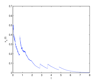
Figure 4: Simulation of one path in Example 5.2

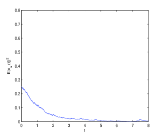
Figure 5: Mean square of 1000 paths in Example 5.2

Example 5.3

Consider the following scalar SDEs with jumps

$$dx(t^{-})=(x(t^{-})-x^{3}(t^{-}))dt+x(t^{-})dB(t)+x(t^{-})dN(t),$$ (5.9)

with the initial value $x(0)=x_{0}\in\mathbb{R}$, where $B(t)$ is a scalar Brownian motion and $N(t)$ is a scalar Poisson process with jump intensity $\lambda=0.1$. We decompose the drift and diffusion coefficient in the form with

$$F_{1}(x)=-2x,\quad F(x)=3x-x^{3},\quad G_{1}(x)=x,\quad G(x)=0,\quad h(x)=x,$$ (5.10)

which means

$$|F_{1}(x)|\vee|G_{1}(x)|\vee|h(x)|=2|x|,\quad\textrm{with}\quad K_{1}=2.$$

Setting $\theta=0$ gives

$$2xF_{1}(x)+(1+\theta)|G_{1}(x)|^{2}=-3x^{2},$$

and

$$2xF(x)+(1+\theta^{-1})|G(x)|^{2}=2x(3x-x^{3})=-2(x^{2}-1.5)^{2}+4.5\leq 4.5.$$

Hence, Assumption 4.4 is satisfied with

$$\bar{\alpha}_{1}=0,\quad\bar{\beta}_{1}=3,\quad\bar{\alpha}_{2}=4.5,\quad\textrm{and}\quad\bar{\beta}_{2}=0.$$ (5.11)

It is easy to check that coefficients of the SDE 5.9 with their decompositions in (5.10) satisfy Assumption 3.1, 3.2 and 3.3 for any $\bar{p}>2$. Applying Theorem 4.5 gives that for any initial value $x_{0}\in\mathbb{R}^{d}$, the solution of SDE 5.9 satisfies

$$\mathop{\lim\sup}\limits_{t\to\infty}\mathbb{E}|x(t)|^{2}\leq\frac{\bar{\alpha}_{1}+\bar{\alpha}_{2}+4\lambda K_{1}^{2}}{\bar{\beta}_{1}-\bar{\beta}_{2}-\lambda(4K_{1}^{2}+1)}\approx 4.69.$$ (5.12)

Moreover, we can choose $\mu(n)=4n^{3}$ and $\varphi(\Delta)=\Delta^{-\varepsilon}$ and let $r=2$, $\bar{\gamma}=2$, $p=50$ as well as $\varepsilon=1/50$ to define the numerical solution $X_{\Delta}(t_{k})$ by the partially truncated EM method. By Theorem 3.11, this solution of truncated EM will converge to the true solution in $\mathcal{L}^{2}$ with convergence rate $1/(1+\bar{\gamma})-r/p\approx 0.2933$. Finally, by Theorem 4.7, for any $\epsilon\in(0,1.3)$, there exists a $\hat{\Delta}\in(0,\Delta^{\ast})$ such that for all $\Delta\in(0,\hat{\Delta})$ and any initial value $x_{0}\in\mathbb{R}^{d}$, the numerical solution satisfies

$$\mathop{\lim\sup}\limits_{k\to\infty}\mathbb{E}|X_{\Delta}(t_{k}^{-})|^{2}\leq\frac{\bar{\alpha}_{1}+\bar{\alpha}_{2}+2\lambda K_{1}(2+K_{1})+\epsilon}{\bar{\beta}_{1}-\bar{\beta}_{2}-2\lambda K_{1}(2+K_{1})-\epsilon}=\frac{6.1+\epsilon}{1.4-\epsilon}.$$

The asymptotic boundedness of the numerical method is shown in Fig 7 and Fig 7.

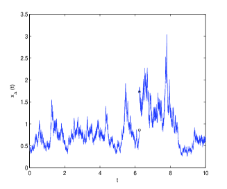
Figure 6: Simulation of one path in Example 5.3

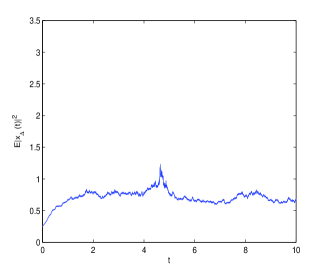
Figure 7: Mean square of 1000 paths in Example 5.3

6 Conclusions and future research

In this paper, the truncated EM method is investigated for SDEs driven by both Brownian motions and Possion jumps. Both the finite time convergence and asymptotic behaviours of the method are studied. The $\mathcal{L}^{r}(r\geq 2)$ strong convergence is proved when the drift and diffusion coefficients satisfy super-linear growth condition and the coefficient for Possion jumps satisfies linear growth condition. When $0<r<2$, we are able to prove the $\mathcal{L}^{r}$ convergence of the methods to SDEs with all the three coefficients allowing to grow super-linearly.

In the future works, we will report on the SDEs driven by Lévy process and the $\mathcal{L}^{r}$ convergence for SDEs whose all the three coefficients can grow super-linearly.

Appendix A Proof of Lemma 3.9

Proof. By the Itô formula and (3.7), we have

$$\mathbb{E}|x(t\wedge\tau_{n})|^{2} \leq|x_{0}|^{2}+\mathbb{E}\int_{0}^{t\wedge\tau_{n}}K_{3}(1+|x(s)|^{2})ds$$

$$\quad+\lambda\mathbb{E}\int_{0}^{t\wedge\tau_{n}}(2x(s)^{T}h(x(s))+|h(x(s))|^{2})ds$$

$$\leq|x_{0}|^{2}+(K_{3}+2\lambda(2K_{1}+K_{1}^{2}))\int_{0}^{t}\mathbb{E}(1+|x(s\wedge\tau_{n})|^{2})ds$$

for any $0<t<T$. The Gronwall inequality shows

$$\mathbb{E}|x(T\wedge\tau_{n})|^{2}\leq C.$$

This implies

$$\mathbb{P}(\tau_{n}\leq T)\leq\frac{C}{n^{2}}.$$

Thus, the proof is complete. $\Box$

Appendix B Proof of Lemma 3.10

Proof. We write $\rho_{\Delta,n}=\rho$ for simplicity. For $0\leq t\leq T$, the Itô formula gives

$$\mathbb{E}|x_{\Delta}(t\wedge\rho)|^{2} =|x_{0}|^{2}+\mathbb{E}\int_{0}^{t\wedge\rho}\Big{(}2x_{\Delta}^{T}(s)f_{\Delta}(\bar{x}_{\Delta}(s^{-}))+|g_{\Delta}(\bar{x}_{\Delta}(s^{-}))|^{2}\Big{)}ds$$

$$\quad+\lambda\mathbb{E}\int_{0}^{t\wedge\rho}\Big{(}2x_{\Delta}^{T}(s)h(\bar{x}_{\Delta}(s^{-}))+|h(\bar{x}_{\Delta}(s^{-}))|^{2}\Big{)}ds$$

$$=|x_{0}|^{2}+\mathbb{E}\int_{0}^{t\wedge\rho}\Big{(}2\bar{x}_{\Delta}^{T}(s)f_{\Delta}(\bar{x}_{\Delta}(s^{-}))+|g_{\Delta}(\bar{x}_{\Delta}(s^{-}))|^{2}\Big{)}ds$$

$$\quad+\mathbb{E}\int_{0}^{t\wedge\rho}2(x_{\Delta}(s^{-})-\bar{x}_{\Delta}(s^{-}))^{T}f_{\Delta}(\bar{x}_{\Delta}(s^{-}))ds$$

$$\quad+\lambda\mathbb{E}\int_{0}^{t\wedge\rho}\Big{(}2x_{\Delta}^{T}(s)h(\bar{x}_{\Delta}(s^{-}))+|h(\bar{x}_{\Delta}(s^{-}))|^{2}\Big{)}ds.$$ (B.1)

By (3.2), we obtain

$$\mathbb{E}\int_{0}^{t\wedge\rho}\Big{(}2x_{\Delta}^{T}(s)h(\bar{x}_{\Delta}(s^{-}))+|h(\bar{x}_{\Delta}(s^{-}))|^{2}\Big{)}ds$$

$$\leq\mathbb{E}\int_{0}^{t\wedge\rho}\Big{(}|x_{\Delta}(s^{-})|^{2}+2|h(\bar{x}_{\Delta}(s^{-}))|^{2}\Big{)}ds$$

$$\leq\mathbb{E}\int_{0}^{t\wedge\rho}\Big{(}|x_{\Delta}(s^{-})|^{2}+4K_{1}^{2}(1+|\bar{x}_{\Delta}(s^{-})|^{2})\Big{)}ds$$

$$\leq 4K_{1}^{2}T+(8K_{1}^{2}T+1)\mathbb{E}\int_{0}^{t\wedge\rho}|x_{\Delta}(s^{-})|^{2}ds+8K_{1}^{2}T\mathbb{E}\int_{0}^{t\wedge\rho}|x_{\Delta}(s^{-})-\bar{x}_{\Delta}(s^{-})|^{2}ds.$$ (B.2)

Substituting this into (B) and applying 3.10, we have

$$\mathbb{E}|x_{\Delta}(t\wedge\rho)|^{2} \leq|x_{0}|^{2}+\int_{0}^{t\wedge\rho}2K_{4}(1+|\bar{x}_{\Delta}(s^{-})|^{2})ds+4\lambda K_{1}^{2}T$$

$$\quad+\mathbb{E}\int_{0}^{t\wedge\rho}2(x_{\Delta}(s^{-})-\bar{x}_{\Delta}(s^{-}))^{T}f_{\Delta}(\bar{x}_{\Delta}(s^{-}))ds$$

$$\quad+\lambda(8K_{1}^{2}T+1)\mathbb{E}\int_{0}^{t\wedge\rho}|x_{\Delta}(s^{-})|^{2}ds+\lambda 8K_{1}^{2}T\mathbb{E}\int_{0}^{t\wedge\rho}|x_{\Delta}(s^{-})-\bar{x}_{\Delta}(s^{-})|^{2}ds$$

$$\leq(|x_{0}|^{2}+2K_{4}T+4\lambda L_{1}^{2}T)+(4K_{4}+\lambda(8K_{1}^{2}T+1))\int_{0}^{t}\mathbb{E}|x_{\Delta}(s\wedge\rho)|^{2}ds$$

$$\quad+(4K_{4}+8\lambda K_{1}^{2}T)\int_{0}^{T}\mathbb{E}|x_{\Delta}(s^{-})-\bar{x}_{\Delta}(s^{-})|^{2}ds$$

$$\quad+2\mathbb{E}\int_{0}^{t\wedge\rho}|x_{\Delta}(s^{-})-\bar{x}_{\Delta}(s^{-})||f_{\Delta}(\bar{x}_{\Delta}(s^{-}))|ds.$$ (B.3)

By Lemma 3.6, we have

$$\int_{0}^{T}\mathbb{E}|x_{\Delta}(s^{-})-\bar{x}_{\Delta}(s^{-})|^{2}ds\leq C.$$

By (3.2), we have

$$\mathbb{E}\int_{0}^{t\wedge\rho}|x_{\Delta}(s^{-})-\bar{x}_{\Delta}(s^{-})||f_{\Delta}(\bar{x}_{\Delta}(s^{-}))|ds$$

$$\leq K_{1}\mathbb{E}\int_{0}^{t\wedge\rho}|x_{\Delta}(s^{-})-\bar{x}_{\Delta}(s^{-})|(1+|\bar{x}_{\Delta}(s^{-})|)ds+I_{5}$$

$$\leq C\Big{(}\mathbb{E}\int_{0}^{t\wedge\rho}|x_{\Delta}(s^{-})-\bar{x}_{\Delta}(s^{-})|^{2}ds+\int_{0}^{t}\mathbb{E}|x_{\Delta}(s\wedge\rho)|^{2}ds+1\Big{)}+I_{5}$$ (B.4)

where

$$I_{5}=\mathbb{E}\int_{0}^{T}|x_{\Delta}(s^{-})-\bar{x}_{\Delta}(s^{-})||F_{\Delta}(\bar{x}_{\Delta}(s^{-}))|ds.$$

Using Lemma (3.8), condition 3.8 and (3.9) gives

$$I_{5} \leq\varphi(\Delta)\int_{0}^{T}\Big{(}\mathbb{E}|x_{\Delta}(s^{-})-\bar{x}_{\Delta}(s^{-})|^{2}\Big{)}^{1/2}ds$$

$$\leq C(\varphi(\Delta))^{2}\Delta^{1/2}=C(\varphi(\Delta)\Delta^{1/4})^{2}\leq C.$$

Hence, we have

$$\mathbb{E}|x_{\Delta}(t\wedge\rho)|^{2}\leq C\Big{(}1+\int_{0}^{t}\mathbb{E}|x_{\Delta}(s\wedge\rho)|^{2}ds\Big{)}.$$

The Gronwall inequality gives

$$\mathbb{E}|x_{\Delta}(T\wedge\rho)|^{2}\leq C,$$

which implies (3.72). Thus, the proof is complete. $\Box$

Appendix C Proof of Lemma 3.18

Proof. Fix any $\Delta\in(0,\Delta^{\ast}]$. Recall that $\mu^{-1}(\varphi(\Delta^{\ast}))\geq 1$, we get $\mu^{-1}(\varphi(\Delta))\geq 1$. For $x\in\mathbb{R}^{d}$ with $|x|\leq\mu^{-1}(\varphi(\Delta))$, by the definition of the truncated function, we obtain the required assertion (3.63). For $x\in\mathbb{R}^{d}$ with $|x|>\mu^{-1}(\varphi(\Delta))$, by (3.16), we have

$$\quad 2x^{T}f_{\Delta}(x)+|g_{\Delta}(x)|^{2}+\lambda(2x^{T}h_{\Delta}(x)+|h_{\Delta}(x)|^{2})$$

$$=2(x-\pi_{\Delta}(x))^{T}f_{\Delta}(x)+2\lambda(x-\pi_{\Delta}(x))^{T}h_{\Delta}(x)$$

$$\quad+2\pi_{\Delta}(x)^{T}f_{\Delta}(x)+|g_{\Delta}(x)|^{2}+2\lambda\pi_{\Delta}(x)^{T}h_{\Delta}(x)+\lambda|h_{\Delta}(x)|^{2}$$

$$\leq\Big{(}\frac{|x|}{\mu^{-1}(\varphi(\Delta))}-1\Big{)}\Big{(}2\pi_{\Delta}(x)^{T}f(\pi_{\Delta}(x))+2\lambda\pi_{\Delta}(x)^{T}h(\pi_{\Delta}(x))\Big{)}+\bar{K}(1+|\pi_{\Delta}(x)|^{2})$$

$$\leq\Big{(}\frac{|x|}{\mu^{-1}(\varphi(\Delta))}-1\Big{)}(\bar{K}(1+|\pi_{\Delta}(x)|^{2}))+\bar{K}(1+|\pi_{\Delta}(x)|^{2})$$

$$=\frac{|x|}{\mu^{-1}(\varphi(\Delta))}\bar{K}(1+|\mu^{-1}(\varphi(\Delta))|^{2})$$

$$=\bar{K}|x|\Big{(}\frac{1}{\mu^{-1}(\varphi(\Delta))}+|\mu^{-1}(\varphi(\Delta))|\Big{)}$$

$$\leq\bar{K}|x|(1+|x|)\leq\bar{K}(1+|x|)^{2}\leq 2\bar{K}(1+|x|).$$

Thus, we complete the proof. $\Box$

Appendix D Proof of Lemma 4.6

Proof. (4.17) is equivalent to the following expression

$$D_{k}+\frac{B}{A-1}\leq A\left(D_{k-1}+\frac{B}{A-1}\right),\quad\textrm{for}\quad k=0,1,2,\cdots.$$

Hence, we have

$$D_{k}+\frac{B}{A-1}\leq A^{k}\left(D_{0}+\frac{B}{A-1}\right).$$

It follows

$$D_{k}\leq A^{k}\left(D_{0}+\frac{B}{A-1}\right)+\frac{B}{1-A}.$$

Recalling $0<A<1$ and taking $k\to\infty$, we obtain the required assertion 4.18. Thus, the proof is complete. $\Box$

References

References

Allen [2007]
E. Allen, Modeling with Itô Stochastic
Differential Equations, Springer,
Dordrecht, 2007.
Mao [2008]
X. Mao, Stochastic Differential Equations and
Applications, Horwood, 2nd edition,
2008.
Higham and Kloeden [2005]
D. J. Higham, P. E. Kloeden,
Numerical methods for nonlinear stochastic
differential equations with jumps,
Numer. Math. 101
(2005) 101–119.
Higham and Kloeden [2006]
D. J. Higham, P. E. Kloeden,
Convergence and stability of implicit methods for
jump-diffusion systems,
Int. J. Numer. Anal. Model. 3
(2006) 125–140.
Higham and Kloeden [2007]
D. J. Higham, P. E. Kloeden,
Strong convergence rates for backward Euler on a
class of nonlinear jump-diffusion problems,
J. Comput. Appl. Math. 205
(2007) 949–956.
Dareiotis et al. [2016]
K. Dareiotis, C. Kumar,
S. Sabanis,
On tamed Euler approximations of SDEs driven by
Lévy noise with applications to delay equations,
SIAM J. Numer. Anal. 54
(2016) 1840–1872.
Kumar and Sabanis [2017]
C. Kumar, S. Sabanis,
On tamed Milstein schemes of SDEs driven by
Lévy noise,
Discrete Contin. Dyn. Syst. Ser. B
22 (2017) 421–463.
Hutzenthaler et al. [2012]
M. Hutzenthaler, A. Jentzen,
P. E. Kloeden,
Strong convergence of an explicit numerical method
for SDEs with nonglobally Lipschitz continuous coefficients,
Ann. Appl. Probab. 22
(2012) 1611–1641.
Higham [2011]
D. J. Higham,
Stochastic ordinary differential equations in applied
and computational mathematics,
IMA J. Appl. Math. 76
(2011) 449–474.
Zhang and Ma [2017]
Z. Zhang, H. Ma,
Order-preserving strong schemes for SDEs with
locally Lipschitz coefficients,
Appl. Numer. Math. 112
(2017) 1–16.
Sabanis [2013]
S. Sabanis,
A note on tamed Euler approximations,
Electron. Commun. Probab. 18
(2013) 1–10.
Hutzenthaler and Jentzen [2015]
M. Hutzenthaler, A. Jentzen,
Numerical approximations of stochastic differential
equations with non-globally Lipschitz continuous coefficients,
Mem. Amer. Math. Soc. 236
(2015) 1–95.
Mao [2015]
X. Mao,
The truncated Euler-Maruyama method for
stochastic differential equations,
J. Comput. Appl. Math. 290
(2015) 370–384.
Mao [2016]
X. Mao,
Convergence rates of the truncated Euler-Maruyama
method for stochastic differential equations,
J. Comput. Appl. Math. 296
(2016) 362–375.
Tan and Yuan [2018]
L. Tan, C. Yuan,
Convergence rates of truncated EM scheme for
NSDDEs,
ArXiv e-prints (2018).
Kumar and Sabanis [2017]
C. Kumar, S. Sabanis,
On explicit approximations for Lévy driven SDEs
with super-linear diffusion coefficients,
Electron. J. Probab. 22
(2017) 1–19.
Yang and Wang [2017]
X. Yang, X. Wang,
A transformed jump-adapted backward Euler method
for jump-extended CIR and CEV models,
Numer. Algorithms 74
(2017) 39–57.
Przybyl owicz [2016]
P. Przybyl owicz,
Optimal global approximation of stochastic
differential equations with additive Poisson noise,
Numer. Algorithms 73
(2016) 323–348.
Mao et al. [2016]
W. Mao, S. You, X. Mao,
On the asymptotic stability and numerical analysis of
solutions to nonlinear stochastic differential equations with jumps,
J. Comput. Appl. Math. 301
(2016) 1–15.
Wang and Gan [2010]
X. Wang, S. Gan,
Compensated stochastic theta methods for stochastic
differential equations with jumps,
Appl. Numer. Math. 60
(2010) 877–887.
Kloeden and Platen [1992]
P. E. Kloeden, E. Platen,
Numerical Solution of Stochastic Differential Equations,
Springer-Verlag, Berlin,
1992.
Platen and Bruti-Liberati [2010]
E. Platen, N. Bruti-Liberati,
Numerical Solution of Stochastic Differential Equations with
Jumps in Finance, Springer-Verlag,
Berlin, 2010.
Guo et al. [2017]
Q. Guo, W. Liu, X. Mao,
R. Yue,
The partially truncated Euler-Maruyama method and
its stability and boundedness,
Appl. Numer. Math. 115
(2017) 235–251.
Bao et al. [2011]
J. Bao, B. Böttcher,
X. Mao, C. Yuan,
Convergence rate of numerical solutions to SFDEs
with jumps,
J. Comput. Appl. Math. 236
(2011) 119–131.
Guo et al. [2018]
Q. Guo, W. Liu, X. Mao,
A note on the partially truncated Euler-Maruyama
method,
Applied Numerical Mathematics
130 (2018) 157–170.