Non-thermodynamic nature of the orbital angular momentum in neutral fermionic superfluids

Abstract

We discuss the orbital angular momentum (OAM) and the edge mass current in neutral fermionic superfluids with broken time reversal symmetry. Recent mean field studies imply that total OAM of a uniform superfluid depends on boundary conditions and is not a thermodynamic quantity. We point out that this does not conflict with thermodynamics, because there is no intensive external field conjugate to OAM with which a uniform superfluid is stable in the thermodynamic limit, in sharp contrast to the orbital magnetization in a non-superfluid system. We establish a simple physical picture for the sensitivity of OAM to boundaries by introducing the notion of “unpaired fermions” and “fermionic Landau criterion” within a mean field description. In order to go beyond the mean field approximation, we perform a density matrix renormalization group calculation and conclude that the mean field understanding is essentially correct.

I introduction

The study of orbital angular momentum (OAM) in a superfluid with broken time reversal symmetry has a long history since the discovery of ³He-A phase Vollhart and Wölfle (1990); Volovik (2003); Leggett (1975, 2006, 2012); Mizushima et al. (2016). In the $p$-wave ³He-A phase, each Cooper pair is expected to carry OAM $\nu=1$, resulting in a bulk OAM proportional to the total number of fermions $N$ in the system. However, the discussions on the magnitude of the total OAM has been controversial and called “intrinsic angular momentum paradox”. At an intuitive level, the OAM is estimated as $L_{z}=\nu\times N/2$ just by counting the total number of Cooper pairs, while OAM could also be estimated as $L_{z}=\nu\times(N/2)\times(\Delta/\varepsilon_{F})$ since the fermions only around the Fermi energy $\varepsilon_{F}$ would be relevant to physical quantities. $\Delta$ is the gap amplitude of the superfluidity. Both of the physical estimations seem to be reasonable, and detailed theoretical calculations predicted various values of the spontaneous OAM corresponding to these physical pictures Vollhart and Wölfle (1990); Volovik (2003); Leggett (1975, 2006, 2012); Mizushima et al. (2016); Ishikawa (1977); Ishikawa et al. (1980); McClure and Takagi (1979); Mermin (1977); Mermin and Muzikar (1980); Volovik (1995); Kita (1996, 1998); Goryo (1998); Anderson and Morel (1961); Volovik (1975); Volovik and Mineev (1976); Cross (1975, 1977); Combescot (1978); Leggett and Takagi (1978); Hall (1985); Liu (1985).

Recently, this problem attracts renewed interest, partly because the chiral superfluidity like ³He-A state is a prototypical example of topological superconductivity/superfluidity  Mizushima et al. (2016); Stone and Anduaga (2008); Sauls (2011); Huang et al. (2014, 2015); Tada et al. (2015); Volovik (2015); Ojanen (2016); Scaffidi and Simon (2015); Tsuruta et al. (2015); Suzuki and Asano (2016). In such a chiral topological state, the edge mass current $J_{\rm edge}$ flows along a sample boundary, which leads to OAM $L_{z}=2J_{\rm edge}\times V$ where $V$ is the sample volume. Interestingly, it has been proposed that the OAM is related to non-dissipative transport phenomena in two-dimensional chiral superfluids Nomura et al. (2012); Gromov and Abanov (2015); Read (2009); Read and Rezayi (2011); Bradlyn et al. (2012); Hoyos et al. (2014); Shitade and Kimura (2014); the thermal Hall conductivity $\kappa_{H}$ is given by temperature derivative of OAM, and the quantization of $\kappa_{H}$ at low temperature which is the hallmark of a chiral superfluid as a symmetry protected topological phase is attributed to the quantized value of the edge mode contribution to OAM Nomura et al. (2012); Gromov and Abanov (2015). Similarly, the Hall viscosity $\eta_{H}$ at zero temperature which is considered as an intrinsic non-dissipative transport quantity in two-dimensions is shown to be proportional to OAM per fermion at and is therefore quantized in chiral superfluids Read (2009); Read and Rezayi (2011); Bradlyn et al. (2012); Hoyos et al. (2014); Shitade and Kimura (2014). The mass current Hall conductivity is also related to the OAM via $\eta_{H}$ Hoyos et al. (2014). Since $\kappa_{H}$ and $\eta_{H}$ are considered as topological intrinsic quantities, their connections to OAM would imply that $L_{z}$ is independent of details of the system such as the gap amplitude $\Delta$ and the Fermi energy $\varepsilon_{F}$.

However, surprisingly, there have been various mean field calculations which show that the spontaneous OAM in a chiral superfluid does depend on boundary conditions of a system and is not an intrinsic quantity  Sauls (2011); Huang et al. (2014, 2015); Tada et al. (2015); Volovik (2015); Ojanen (2016); Scaffidi and Simon (2015); Tada (2015); Nagato et al. (2011); Lederer et al. (2014); Bouhon and Sigrist (2014). This is, on one hand, quite counter-intuitive, since it has been widely regarded that OAM is a thermodynamic quantity and should be independent of non-thermodynamic details such as boundary conditions and shapes of a system. This can be inferred from the well-known formula for the total OAM,

$$L_{z}=-\frac{\partial F({\Omega_{z}})}{\partial\Omega_{z}},$$ (1)

where $F(\Omega_{z})$ is the free energy in the rotating frame with the angular velocity $\Omega_{z}$ along $z$-axis Landau and Lifshitz (1984). On the other hand, the sensitivity of OAM to boundaries would be rather natural, since the origin of spontaneous OAM in a chiral superfluid is mainly the edge mass current and such a current could be influenced by details of boundaries along which the current flows. For example, we may expect that edge mass current depends on roughness of the sample surface. Indeed, this was shown to occur within mean field calculations Sauls (2011); Tada (2015); Nagato et al. (2011); Lederer et al. (2014). It was also demonstrated that directions of edge mass current can be even reversed depending on sample shapes Bouhon and Sigrist (2014). Similar reversal of edge mass current is possible at a domain boundary between superfluids with positive and negative chiralities Tsutsumi (2014); Tada (2018). All the contributions to the energy from boundary conditions and system shapes themselves are at most proportional to the surface area in a system with short range interactions.

One can compare the OAM in superfluids with spontaneous orbital magnetization (OM) in non-superfluid systems, and will find a qualitative difference between these two quantities. Total spotaneous OM for a finite size system is simply proportional to total OAM at zero magnetic flux density, $M_{z}=-\mu_{B}L_{z}$, as an operator in an appropriately chosen gauge where $\mu_{B}$ is the Bohr magneton com (a). Although one might expect that the spontaneous OM is also a non-thermodynamic quantity which depends on boundaries or shapes, it is a thermodynamic quantity and the well known formula,

$$M_{z}=-\frac{\partial F(B_{z})}{\partial B_{z}},$$ (2)

is a thermodynamic relation, where $B_{z}$ is the uniform magnetic flux density com (b); Banerjee et al. (1998). Indeed, these have been proved to be true in non-interacting systems Angetescu et al. (1975); Macris et al. (1988); Briet et al. (2012), and free energy density in interacting systems have also been discussed extensively Ruelle (1999); Lieb and Seiringer (2010). Therefore, the non-thermodynamic nature of spontaneous OAM discussed in the previous studies would be a characteristic property only in superfluids.

Experimentally, direct observations of OAM and corresponding edge mass currents are challenging issues. For example, there have been a limited number of experimental reports on the intrinsic angular momentum paradox in the ³He-A phase Manninen et al. (1996); Bevan et al. (1997); pro , and the magnitude of the edge charge current in the candidate chiral $p$-wave superconductor Sr₂RuO₄ is extremely small compared with a theoretical estimation Hicks et al. (2010); Scaffidi and Simon (2015). If OAM and edge currents are boundary sensitive quantities, careful discussions will be required for an experimental detetction.

Although there have been many calculations of spontaneous OAM and corresponding edge mass current for concrete models of superfluids within mean field approximations  Sauls (2011); Huang et al. (2014, 2015); Tada et al. (2015); Volovik (2015); Ojanen (2016); Scaffidi and Simon (2015); Tsuruta et al. (2015); Suzuki and Asano (2016); Tada (2015); Nagato et al. (2011); Lederer et al. (2014); Bouhon and Sigrist (2014), a comprehensive understanding especially on connections to thermodynamics has not been well established. Therefore, it is desirable to develop a simple understanding on the physical reason why OAM in superfluids can depend on non-thermodynamic details, and obtain an intuitive picture. In this study, we point out that the OAM, especially the spontaneous OAM, in a superfluid is not a thermodynamic quantity by focusing on absence of a thermodynamic limit under rotation and roles of Hess-Fairbank effect under an artificial magnetic flux density. Then, we establish a simple physical picture for the non-thermodynamic nature of the OAM within mean field descriptions, where two important notions, “unpaired fermions” and “fermionic Landau criterion”, are introduced. In order to go beyond the mean field approximations, we perform a non-perturbative numerical calculation by using the infinite density matrix renormalization group (iDMRG) White (1992); Schollwöck (2005, 2011); pap (a, b); Kjäll et al. (2013). It is concluded that the mean field understanding is essentially correct.

II non-thermodynamics of OAM in neutral superfluid

In this section, we discuss whether or not OAM (especially spontaneous OAM) in a uniform superfluid can be described within the standard thermodynamics. Although this will be an elementaly discussion, to the best of our knowledge, it has never been explicitly considered in the context of the spontaneous OAM in chiral superfluids. This may be a reason for the controversial discussions on the OAM, and therefore we will clarify some important points here.

II.1 General discussion

The extensive thermodynamic free energy $F^{\rm TD}_{V}$ for volume $V$ can be derived from the statistical mechanical free energy density in the thermodynamic limit $f_{\infty}$,

$$F^{\rm TD}_{V}=V\times f_{\infty}.$$ (3)

If $F^{\rm TD}_{V}$ is well-defined in the presence of $\Omega_{z}\neq 0$ or $B_{z}\neq 0$, Eq. (1) or  (2) becomes a thermodynamic relation. Since a thermodynamic free energy is stable to non-extensive perturbations such as boundary conditions and shapes, a physical extensive quantity obtained from $F^{\rm TD}_{V}$ should also be thermodynamic. However, in general, it is a non-trivial problem whether or not a microscopic model has a well-defined thermodynamic limit and thermodynamics can be applied to the system. Indeed, the previous mean field studies may imply that Eqs. (1) and  (2) for a uniform superfluid are not thermodynamic relations  Sauls (2011); Huang et al. (2014, 2015); Tada et al. (2015); Volovik (2015); Ojanen (2016); Scaffidi and Simon (2015); Tsuruta et al. (2015); Suzuki and Asano (2016); Tada (2015); Nagato et al. (2011); Lederer et al. (2014); Bouhon and Sigrist (2014).

For a general system, we would naively expect that an extensive quantity $M$ is stable to non-extensive perturbations if and only if it is derived from a thermodynamic free energy. Indeed, if the thermodynamic free energy is obtained in the presence of a conjugate intensive field $h$ to $M$, we have

$$M^{\rm TD}_{V}(h) =-\frac{\partial F^{\rm TD}_{V}(h)}{\partial h},$$ (4)

where $M^{\rm TD}_{V}$ is the thermodynamic value of the statistical mechanical quantity $M$  com (c); Lebowitz (1968). Similarly, if the statistical mechanical expectation value $\langle M\rangle_{V}$ is robust to non-extensive perturbations, the statistical mechanical free energy $F_{V}$ with the intensive conjugate field $h\neq 0$ obtained as

$$F_{V}(h)-F_{V}(0) =-\int_{0}^{h}dh^{\prime}\langle M\rangle_{V}(h^{\prime})$$ (5)

will also be stable to the perturbations, if possible changes in $F_{V}(0)$ by the perturbations are at most $o(V)$ com (d). For such a stable $F_{V}(h)$, one would naively expect existence of a well defined thermodynamic limit.

An important subtle point in OAM is that the OAM operator itself is not extensive Cross (1977); Leggett and Takagi (1978); com (e). For a system on $V\subset{\mathbb{R}}^{3}$, the OAM operator is defined as

$$L_{z} =\int_{V}\psi^{\dagger}[\mbox{\boldmath$r$}\times\mbox{\boldmath$p$}]_{z}\psi d^{3}x=\int_{V}[\mbox{\boldmath$r$}\times\mbox{\boldmath$j$}]_{z}d^{3}x,$$ (6)

$$\mbox{\boldmath$j$}(\mbox{\boldmath$r$}) =-i(\psi^{\dagger}\nabla\psi-\nabla\psi^{\dagger}\psi)/2,$$ (7)

where $\mbox{\boldmath$p$}_{j}=-i\nabla_{j}$ and $j$ is the mass current density. Or equivalently, in the first quantization form,

$$L_{z} =\sum_{i=1}^{N}\mbox{\boldmath$r$}_{i}\times\mbox{\boldmath$p$}_{i}=\int_{V}[\mbox{\boldmath$r$}\times\mbox{\boldmath$j$}]_{z}d^{3}x,$$ (8)

$$\mbox{\boldmath$j$}(\mbox{\boldmath$r$}) =\sum_{i=1}^{N}\{\delta(\mbox{\boldmath$r$}-\mbox{\boldmath$r$}_{i}),\mbox{\boldmath$p$}_{i}\}/2.$$ (9)

Although it is not trivial from these expressions, its expectation value at equilibrium scales as $\langle L_{z}\rangle_{V}=O(V)$, if an equilibrium state is well-defined. This is because $\mbox{\boldmath$j$}(\mbox{\boldmath$r$})$ is usually localized around the boundary of $V$ in such a state Tada and Koma (2016), and the above expressions can be reduced to

$$\langle L_{z}\rangle_{V} \simeq\int_{\partial V}[\mbox{\boldmath$r$}\times\mbox{\boldmath$J$}_{\rm edge}]_{z}d^{2}x_{\parallel},$$ (10)

$$\mbox{\boldmath$J$}_{\rm edge}(\mbox{\boldmath$r$}_{\parallel}) =\int\langle\mbox{\boldmath$j$}(\mbox{\boldmath$r$})\rangle_{V}dx_{\perp},$$ (11)

where $\mbox{\boldmath$J$}_{\rm edge}$ is the net edge current which are the integral of $\langle\mbox{\boldmath$j$}\rangle_{V}$ over the perpendicular direction $x_{\perp}$ to the surface com (f). Then, it is clear that $\langle L_{z}\rangle_{V}=O(V^{2/3})\times O(V^{1/3})=O(V)$.

We note that it is impossible to express the operator $L_{z}$ as a sum of local “OAM density operator” which is translationally symmetric Cross (1977); Leggett and Takagi (1978). This can be understood as follows. Suppose that there exists a local OAM density operator of the form $\mbox{\boldmath$l$}(\mbox{\boldmath$r$})=[\psi^{\dagger}(\mbox{\boldmath$r$})\hat{\mbox{\boldmath$l$}}(\nabla)\psi(\mbox{\boldmath$r$})+({\rm h.c.})]$ where $\hat{\mbox{\boldmath$l$}}$ is independent of $r$. We expand $\hat{l}_{j}=a_{1j}+a_{2jk}\nabla_{k}+\cdots$ where $a_{1j},a_{2jk},\cdots\in{\mathbb{C}}$. Then it is easy to see that there is no solution for the commutation relation $[l_{i}(\mbox{\boldmath$r$}),l_{j}(\mbox{\boldmath$r$}^{\prime})]=i\delta(\mbox{\boldmath$r$}-\mbox{\boldmath$r$}^{\prime})\epsilon_{ijk}l_{k}(\mbox{\boldmath$r$})$. Therefore, the operator $\mbox{\boldmath$l$}(\mbox{\boldmath$r$})$ does not exist com (g); Bianco and Resta (2013); Marrazzo and Resta (2016). This is in sharp contrast to the familiar spin magnetization operator which can be equivalently expressed either of the form $\int_{V}d^{3}x\mbox{\boldmath$s$}(\mbox{\boldmath$r$})$ or $\int_{V}d^{3}x[\mbox{\boldmath$r$}\times(\nabla\times\mbox{\boldmath$s$}(\mbox{\boldmath$r$}))]$ with $\mbox{\boldmath$s$}(\mbox{\boldmath$r$})=\psi^{\dagger}\mbox{\boldmath$\sigma$}\psi/2$. These are consistent with our naive expectation that spin is an internal degrees of freedom which has the spatial position independent generator of SU(2) symmetry, while an orbital motion is an spatially extended object and therefore there is no local, translationally symmetric generator of SO(3) rotational symmetry.

In the following, we will consider several theoretical setups in which OAM might possibly be obtained by derivative of a thermodynamic free energy; we introduce two kinds of external fields, a uniform rotation with or without additional confinement potentials corresponding to Eq.(1), and an artificial constant magnetic flux density corresponding to Eq.(2). In each case, we explain that $F^{\rm TD}_{V}(h)$ is not obtained for a superfluid with a uniform density, and OAM cannot be regarded as a thermodynamic quantity.

II.2 System under rotation

The robustness of $\langle M\rangle_{V}$ is guaranteed by the existence of a thermodynamic limit of $f_{V}(h)=F_{V}(h)/V$ under the intensive conjugate field $h$ for fixed $N/V$, which is often implicitly assumed in condensed matter physics. Although this assumption is indeed satisfied in many systems, there are several important exceptions and a system of particles under a uniform rotation, for example, confined in a cylinder of radius $R$ is the case  Widom (1968); Lebowitz (1968); com (h); Avron and Herbst (1977); Blanc and Monneau (2002). This is simply because the centrifugal potential $V_{\rm cen}\propto-(\Omega_{z}r_{\perp})^{2}$ ($r_{\perp}$ is the in-plane distance from the rotation axis) will push the particles onto the boundary of a system and velocities of those particles $\Omega_{z}R$ will be infinitely fast when the system size $R$ becomes $R\rightarrow\infty$ with keeping $\Omega_{z}\neq 0$. Indeed, it is easy to show that such a system described by Schrödinger Hamiltonian with a stable, short-range interaction does not have stability of Hamiltonian of the second kind, i.e. ${}^{\neg}(H>{\rm const}\times V)$, and therefore does not have a thermodynamic limit when the particles are confined in a rigid wall container Widom (1968). For example, we consider variational single particle wavefunctions

$$\psi_{j}(r_{j},\theta_{j},z_{j})\simeq e^{il_{j}\theta_{j}}\tilde{\psi}_{j}(r_{j}),$$ (12)

where $l_{j}=\Omega_{z}/\Omega_{j}$ with $\Omega_{j}=1/mR_{j}^{2}$ and the particle mass $m$. $\tilde{\psi}_{j}(r_{j})$ is localized at $r_{j}=R_{j}=O(R)$ and satisfies a given boundary condition at $r_{j}=R$. Although we only consider particular values of $\Omega_{z}$ for which $\psi_{j}$ is consistent with a given boundary condition on $\theta_{j}$, there are many such $\Omega_{z}$s when $\Omega_{0}=1/mR^{2}$ is sufficiently small. We then construct an anti-symmmetric many-body wavefunction $\Psi_{\rm var}$ for $N$ particles from these single particle wavefunctions, which obviously gives $\langle\Psi_{\rm var}|H|\Psi_{\rm var}\rangle\sim-I_{0}\Omega_{z}^{2}/2=O(V^{5/3})$ with $I_{0}=mNR^{2}$ in the leading order. It is noted that the expectation value of a stable, short range interaction term in the Hamiltonian is at most $O(V)$, and therefore it is irrelevant here.

For such a system to have a thermodynamic limit, one needs to keep $\Omega_{z}R=O(1)$ at a fixed value when taking $R\rightarrow\infty$, which means that the angular velocity $\Omega_{z}$ is no longer an intensive field conjugate to OAM  com (i); Davies et al. (1996); Duffy and Ottewill (2003); Mameda and Yamamoto (2016). Therefore, Eq. (1) is an equation which holds only in a small size system and is not a thermodynamic equation. In fact, for such a case, the coupling term in the free energy is $-\Omega_{z}\langle L_{z}\rangle=O(R^{-1})O(V)=O(V^{2/3})$ when OAM is $O(V)$, and this energy gain is comparable with possible surface perturbations and therefore cannot guarantee thermodynamic nature of OAM. Note that it could be considered that the state with a uniform density distribution Leggett (1970, 1998) is metastable (or non-equilibrium) and is not a true equilibrium/ground state of a rotating three-dimensional system.

One may expect that the Hamiltonian can be made stable for fixed $\Omega_{z}=O(1)$ by use of a mathematical trick of introducing an additional confinement potential such as $V_{\rm con}=C_{n}r_{\perp}^{n}$, and taking an appropriate limit of $C_{n}\downarrow 0$. This might reproduce the desired thermodynamic limit of the original free energy, if $V_{\rm con}$-dependence of the free energy density could be removed. In order to do so, we wish to take the limit, $\lim_{C_{n}\downarrow 0}\lim_{N\uparrow\infty}F_{N}(\Omega_{z})/N$ for fixed $\Omega_{z}=O(1)$. However, for such a Hamiltonian with a confinement potential, one needs to take a scaling limit of $C_{n}$ and $N$ to have an extensive free energy. For example $n=2$, the kinetic Hamiltonian can be written as $(\mbox{\boldmath$p$}-\mbox{\boldmath$A$})^{2}/2m+m\tilde{\Omega}_{z}^{2}r_{\perp}^{2}/2$ where $\mbox{\boldmath$A$}=m\Omega\times\mbox{\boldmath$r$}$ and $\tilde{\Omega}_{z}^{2}=(C_{2}-\Omega_{z}^{2})>0$ with an appropriately chosen $C_{2}$. Although $C_{2}\downarrow 0$ limit cannot be taken for keeping the Hamiltonian with a fixed $\Omega_{z}\neq 0$ stable, a scaling limit is required similarly to other $n$ cases. Indeed, to have an extensive free energy $F_{N}\propto N$ of the fermion model, one needs to keep $N_{2}\tilde{\Omega}_{z}^{2}=O(1)$ and the free energy density will depend on the value of $N_{2}\tilde{\Omega}_{z}^{2}$, where $N_{2}$ is the total number of particles divided by the length of the system in $z$-direction Yoshioka and Fukuyama (1992). Therefore, we cannot take the desired thermodynamic limit where the free energy density is well-defined and $V_{\rm con}$-independent, even if the mathematical trick of an additional confinement potential is used. The special case $\tilde{\Omega}_{z}=0$ for which the scaling limit is not required will be discussed in the next section.

In summary, we have seen that the angular velocity is not an intensive field conjugate to OAM. Therefore, we conclude that, in general, OAM in a system with a uniform particle density is not a thermodynamic quantity.

II.3 System with constant artificial magnetic flux

II.3.1 Non-interacting case

In the previous section, we have seen that OAM in a uniform system is generally non-thermodynamic. However, this does not necessarily mean that spontaneous OAM at zero external field $\Omega_{z}=0$ is sensitive to non-extensive perturbations. As mentioned in Sec. I, OAM is equivalent to OM at zero field as an operator, and the latter is thermodynamic in metals and insulators. If we consider a neutral system minimally coupled with an artificial gauge field $\mbox{\boldmath$A$}=m\mbox{\boldmath$\Omega$}\times\mbox{\boldmath$r$}\equiv\mbox{\boldmath$B$}\times\mbox{\boldmath$r$}/2$, the Hamiltonian is formally equivalent to the charged particles under a constant magnetic flux density in the symmetric gauge. Or equivalently, we can introduce $V_{\rm con}=m(\Omega_{z}r_{\perp})^{2}/2$ as a mathematical trick to make the Hamiltonian under rotation stable. We note that a gauge invariant Hamiltonian $H$ now has the stability $H>{\rm const}\times V$ and translational symmetry if combined with a suitable gauge transformation, and we can take the desired limit $\lim_{V\uparrow\infty}F_{V}(B_{z})/V$ for a fixed intensive field $B_{z}\neq 0$ in this case. If the “charged” system under uniform $B_{z}$ has a thermodynamic limit, spontaneous OAM in a neutral system obtained as the limit of $B_{z}\downarrow 0$ (or $B_{z}\uparrow 0$) will also be thermodynamic. Indeed, this is true for non-superfluids and spontaneous OM/OAM obtained so will be a thermodynamic quantity  Angetescu et al. (1975); Macris et al. (1988); Briet et al. (2012); Ruelle (1999); Lieb and Seiringer (2010). We will give a brief explanation on the existence of the thermodynamic limit in Appendix A.

Similarly, one might expect that OAM in a neutral superfluid should be thermodynamic as well. Unfortunately, this expectation is not correct, because for a Hamiltonian of a uniform superfluid under a constant artificial magnetic flux density $B_{z}$, derivative of the free/ground state energy with respect to $B_{z}$ does not give the desired OM. To see this, for simplicity, let us consider a non-interacting fermionic Hamiltonian with a uniform $s$-wave gap function $\Delta_{0}$ as a U(1) symmetry breaking field, $H=\int d^{3}x\psi^{\dagger}[(\mbox{\boldmath$p$}-\mbox{\boldmath$A$})^{2}/2m]\psi+\Delta_{0}\int d^{3}x\psi^{\dagger}_{\uparrow}\psi^{\dagger}_{\downarrow}+({\rm h.c.})$. This Hamiltonian is not gauge invariant and does not have translation symmetry, and therefore existence of a thermodynamic limit in the presence of $B_{z}\neq 0$ is not guaranteed. Indeed, the induced current is given by $\langle\mbox{\boldmath$j$}\rangle\simeq-\langle(\psi^{\dagger}\psi\rangle/m)\mbox{\boldmath$A$}\propto\mbox{\boldmath$B$}\times\mbox{\boldmath$r$}$, and OAM per volume and free energy density diverge at $V\rightarrow\infty$, which is unphysical com (j). The reason for the divergence is very simple; physically, the dangerous behavior of $\langle\mbox{\boldmath$j$}\rangle$ comes from the fact that a uniform real magnetic flux density cannot be realized in superconductors because of the Meissner effect where electromagnetic field is determined by the Maxwell equation. The introduction of the constant artificial $B$-field into the Hamiltonian corresponds to an implicit assumption that there is no Meissner or Hess-Fairbank effect. Such an unphysical assumption results in a huge energy cost, leading to the superextensive free energy $F_{V}$.

For a system defined on a cube with the volume $V=L^{3}$, the superextensive $f_{V}(B)$ behaves as $f_{V}(B)=\tilde{f}(LB)$ where $\tilde{f}$ is a scaling function which is nearly independent of $V$. This is because the additional energy density due to the $B$-field is $B_{z}\langle M_{z}\rangle_{V}/L^{3}\sim B_{z}^{2}\int d^{3}x(x^{2}+y^{2})/L^{3}\sim(B_{z}L)^{2}$, where we have used $\langle\mbox{\boldmath$j$}\rangle_{V}\sim\mbox{\boldmath$A$}=\mbox{\boldmath$B$}\times\mbox{\boldmath$r$}/2$. This scaling behavior is also seen in lattice models. Here, we consider a two-dimensional square lattice of $V=L^{2}$ with open boundaries and spinful fermions at half filling with a fixed uniform $s$-wave gap function as a simple example,

$$H=\sum_{\langle i,j\rangle,\sigma}-te^{iA_{ij}}c_{i\sigma}^{\dagger}c_{j\sigma}+\sum_{i}[\Delta_{0}c_{i\uparrow}^{\dagger}c_{i\downarrow}^{\dagger}+({\rm h.c.})].$$ (13)

The vector potential $A_{ij}$ describes a constant magnetic flux density $B_{z}$ in the symmetric gauge. We show the ground state energy density $\epsilon_{V}(B_{z})=\langle H\rangle_{V}(B_{z})/V$ in Fig.1. $\epsilon_{V}(B_{z})$ has a strong size dependence, and all the data collapse into a single curve in the scaling plot, $\epsilon_{V}(B_{z})=\tilde{\epsilon}(B_{z}L)$. For small $B_{z}L$, the scaling function behaves as $\tilde{\epsilon}(B_{z}L)\sim(B_{z}L)^{2}$ as expected from the above discussion for a continuum system. The scaling behavior clearly shows the absence of the thermodynamic limit at a fixed $B_{z}\neq 0$.

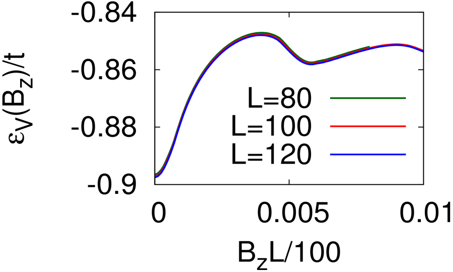
Figure 1: (Left panel) The ground state energy density at $\Delta_{0}=0.6t$ for different system sizes. The dimensionless magnetic flux density is $B_{z}=\phi/2\pi$ where $\phi$ is the flux per plaquette of the square lattice. (Right panel) The ground state energy density in the scaling plot.

Finally, we note that, in a realistic charged superconductor with electromagnetic fields described by the Maxwell equation, the Meissner effect arises from the combination of (i) a response of electrons to a given vector potential and (ii) dynamics of electromagnetic fields in presence of a given electron current. Note that the two contributions (i) and (ii) to the total edge current are spatially separated with different length scales, the coherence length for (i) and the penetration depth for (ii). In the present study, the artificial vector field is a given fixed field and we do not consider its dynamics. On the other hand, the current density as the response (i) should be essentially proportional to the given artificial vector potential in superfluids, which we call “strong diamagnetic response”. It is noted that the induced current density is not necessarily localized at a boundary for a general vector field.

II.3.2 Interacting case

Now we turn to interacting systems under a physically reasonable assumption. In an interacting system, there are two ways for describing a uniform superfluid, one with explicit U(1) symmetry breaking and the other with conserved U(1) symmetry  com (k); Shimizu and Miyadera (2001). In both descriptions, the strong diamagnetic response, i.e. Meissner or Hess-Fairbank effect is a necessary condition for the superfluidity. Then, the assumption is that there exists the strong diamagnetic response where the current density is essentially proportional to a given vector potential, when (i) a uniform U(1) symmetry breaking field $\Delta_{0}$ is introduced into the Hamiltonian, or (ii) there is a uniform long range order of the particle number U(1) symmetry in the absence of $\Delta_{0}$. The uniform long range order is defined as

$$\sigma_{\rm C} =\lim_{V\uparrow\infty}\sqrt{\langle m_{\rm C}^{2}\rangle_{V}},$$ (14)

$$m_{\rm C} =\frac{1}{V}\int_{V}d^{3}x[\psi_{\uparrow}d(-i\nabla)\psi_{\downarrow}+({\rm h.c})],$$ (15)

where $m_{\rm C}$ is the uniform Cooper pair order parameter with a form factor $d=1$ for $s$-wave, $d\sim(p_{x}+ip_{y})$ with $p_{j}=-i\partial_{j}$ for chiral $p$-wave, and so on. This assumption is widely accepted and guarantees presence of the Meissner or Hess-Fairbank effect. The real Meissner effect is realized when combined with the Maxwell equation, but the present artificial vector potential is simply a given field, $|\mbox{\boldmath$A$}|\propto|\mbox{\boldmath$r$}|$. It should be noted that two approaches corresponding to (i) and (ii) are equivalent for evaluating gauge invariant quantities per volume, if there exist the thermodynamic limits for both cases. Corresponding to the two approaches, we consider interacting superfluids in two ways in the following.

In the first scheme (i), we describe a superfluid as a global U(1) symmetry broken state, where an introduced U(1) symmetry breaking field $\Delta_{0}$ must be turned off after the thermodynamic limit is taken. In this case, from the above assumption, there exists a contribution to the current from the symmetry breaking field and $\langle\mbox{\boldmath$j$}\rangle$ should contain a term essentially proportional to $A$. Similarly to the non-interacting case, this leads to an unphysical divergence of the free energy density, since the symmetry breaking field should be kept constant when the thermodynamic limit is taken. Physically, the Hamiltonian with a constant $B_{z}$-field would correspond to a vortex state or a normal (non-superfluid) state. Therefore, if necessary, one might need to introduce new corresponding symmetry breaking field which is different from the uniform field $\Delta_{0}$.

In the other scheme (ii), we do not introduce a symmetry breaking field into the Hamiltonian, and the U(1) symmetry is strictly kept in both finite and infinite volume systems, although we assume that the system has the uniform U(1) long range order in the absence of $B$-field. In this case, there exists the thermodynamic limit of the free energy density under the uniform artificial $B$-field, since the Hamiltonian is translationally invariant if combined with an appropriate gauge transformation. (See Appendix A for a brief discussion.) This means that there is no U(1) long range order, since if it were there, the strong diamagnetic response will lead to a divergent free energy density. Therefore, we conclude that a constant $B$-field will suppress the pre-existing uniform U(1) long range order. The absence of the strong diamagnetic response can also be understood from the Bloch’s theorem which excludes a macroscopic current in a ground state/equilibrium for a U(1) symmetric system Tada and Koma (2016). Besides, the suppression of the uniform long range order may be consistent with a variant of the Elitzur’s theorem for a fixed gauge field configuration derived in Ref. Tada and Koma (2016), according to which the long range order $\sigma_{\rm C}$ vanishes for almost all gauge field configurations. Although we have assumed that $\sigma_{\rm C}\neq 0$ for the specially chosen gauge $\mbox{\boldmath$A$}=0$ in the absence of $B$-field, a gauge field corresponding to the constant $B$-field is no longer compatible with a uniformly Cooper paired state. This is physically reasonable, since one would expect a vortex state or a normal (non-superfluid) state for Hamiltonian with the uniform $B$-field. There might arise a new long range order such as a vortex state once a uniform $B$-field is introduced into the Hamiltonian, or any long range order of U(1) symmetry might get suppressed.

It is important to realize that the state at $B_{z}=0$ and that at $B_{z}\neq 0$ are physically different states in distinct “phases”, because only the former has the uniform U(1) long range order. The quantity we are interested in this study is $l_{0}=\lim_{\Delta_{0}\rightarrow 0}\lim_{V\rightarrow\infty}\langle L_{z}\rangle_{V}(B_{z}=0)/V=\lim_{\Delta_{0}\rightarrow 0}\lim_{V\rightarrow\infty}\partial f_{V}(B_{z}=0,\Delta_{0})/\partial B_{z}$, while the latter state gives different quantities $l_{\pm}=-\partial f_{\infty}(B_{z}\rightarrow\pm 0)/\partial B_{z\pm}$  com (l); Sato and Fujimoto (2016). As already mentioned, $l_{0}$ and $l_{\pm}$ are expectation values of $L_{z}$ at different states. Although $l_{\pm}$ is a thermodynamic quantity by definition, $l_{0}$ is not directly related to $f_{\infty}$ and is not thermodynamic in this sense. We note that $f_{V}(B_{z},\Delta_{0})$ for general $(B_{z},\Delta_{0})$ contains a scaling term $\tilde{f}(B_{z}L,\Delta_{0})$ and diverges as $V\rightarrow\infty$ except for $(B_{z}=0,\Delta_{0})$ or $(B_{z},\Delta_{0}=0)$. It is also noted that the discussions based on the two schemes (i) and (ii) for describing a superfluid are consistent, as expected.

In summary, we have seen that thermodynamic limits of the free energy density do not exist in several theoretical setups which could seemingly realize the desired uniform superfluid state. As a result, the OAM in a neutral superfluid is not a thermodynamic quantity at some value of external (rotation/artificial flux) fields, although it is usually extensive and seemingly thermodynamic. Therefore, it can depend on non-thermodynamic details such as boundary conditions. In the next section, we will demostrate a physical picture on how OAM is affected by non-extensive perturbations.

III mean field description of fragile OAM

III.1 Unpaired fermions and fermionic Landau criterion

In the previous section, we have explained that spontaneous OAM of a neutral superfluid is not related to thermodynamic free energy. Then, it is important to develop a physical understanding on behaviors of OAM in the presence of non-extensive perturbations. In this section, we discuss a mean field understanding at zero external rotation or $B$-field which has potential applicability to a large class of neutral superfluids. This part is based on the recent progress Huang et al. (2015); Tada et al. (2015); Volovik (2015); Ojanen (2016); Tada (2018), and here we establish an intuitively clear picture for the seemingly non-trivial sensitivity of OAM.

In order to demonstrate the essential physics, we consider a two-dimensional $d+id$-wave superfluid confined by a rotationally symmetric potential $V_{\rm con}$ as a simple example. We mainly focus on the weak coupling BCS states where edge states are topological and gapless. The argument can also apply to rotationally asymmetric systems and in principle to the strong coupling BEC states with some modifications, when OAM is determined by an edge mass current. The mean field Hamiltonian with the rotationally symmetric confinement potential reads,

$$H =\int d^{2}x\psi_{\sigma}^{\dagger}\Bigl{(}\frac{\mbox{\boldmath$p$}^{2}}{2m}-\mu+V_{\rm con}\Bigr{)}\psi_{\sigma}$$

$$\quad+\Delta_{0}k_{F}^{-2}\int d^{2}x\psi^{\dagger}_{\uparrow}(p_{x}+ip_{y})^{2}\psi^{\dagger}_{\downarrow}+({\rm h.c.}),$$ (16)

where $p_{j}=-i\nabla_{j}$. $k_{F}$ is the Fermi momentum in the normal state, and $\Delta_{0}$ is the symmetry breaking field. In this section, the confinement potential is zero in the bulk of the system, $V_{\rm con}(r\ll R)=0$, and infinitely large outside of the system, $V_{\rm con}(r\gg R)=\infty$, where $R$ is the system radius. We expand the field operator as $\psi_{\sigma}(r,\theta)=\sum_{ml}c_{ml\sigma}\phi_{ml}(r,\theta)$ by using the single particle eigenfunctions of $[\mbox{\boldmath$p$}^{2}/2m-\mu+V_{\rm con}]$. The Hamiltonian is rewritten into a Bogoliubov-de Gennes form,

$$H =\sum_{m,l}\left[\begin{array}[]{c}c^{\dagger}_{m,l+2,\uparrow}\\ c_{m,-l,\downarrow}\end{array}\right]^{T}\left(\hat{H}_{\rm BdG}^{(l)}\right)_{mm^{\prime}}\left[\begin{array}[]{c}c_{m^{\prime},l+2,\uparrow}\\ c^{\dagger}_{m^{\prime},-l,\downarrow}\end{array}\right].$$ (21)

We first consider a smooth confinement potential $V_{\rm con}(r)$ which increases smoothly around $r\sim R$ with a length scale $\xi_{\rm con}$ which satisfies $\xi_{\Delta}=v_{F}/\Delta_{0}\ll\xi_{\rm con}\ll R$. The total OAM at $T=0$ is easily calculated as Tada et al. (2015); Prem et al. (2017)

$$\langle L_{z}\rangle_{V} =2\times\frac{\langle N\rangle_{V}}{2}-\frac{1}{2}\sum_{l}(l+1)\eta_{l},$$ (22)

$$\eta_{l} =\sum_{n}{\rm sgn}\varepsilon_{n}{(l)},$$ (23)

where $\eta_{l}$ is the spectral asymmetry of the BdG Hamiltonian $H_{\rm BdG}^{(l)}$ for which eigenvalues are $\{\varepsilon_{n}{(l)}\}$. Within the semi-classical approximation which can be valified for $\Delta_{0}\ll\varepsilon_{F}$, OAM at zero temperature is reduced to

$$\langle L_{z}\rangle_{V} \simeq 2\times\frac{\langle N\rangle_{V}}{2}-\frac{1}{2}\sum_{j=1,2}\bigl{(}Rk_{Fj}\bigr{)}^{2}.$$ (24)

Here, we have introduced Fermi wavenumbers of the two one-dimensional edge modes, $k_{F1}=-k_{F2}(k_{F1}\leq k_{F2})$, which are defined as $Rk_{Fj}=l_{j}$ with the vanishing eigenvalues of the edge modes, $\varepsilon_{n}(l_{j})\simeq 0$. Since $\xi_{\Delta}=v_{F}/\Delta_{0}\ll\xi_{\rm con}$, within the semi-classical approximation, the confinement potential can be treated as a constant energy shift $\varepsilon_{F}\rightarrow\varepsilon_{F}^{\prime}=\varepsilon_{F}-V_{\rm con}(r=R)$ for the edge modes localized in the relatively low particle density region $|r-R|\lesssim\xi_{\rm con}$. Then the edge mode Fermi wavenumber is given by $k_{F1,2}=\pm k_{F}^{\prime}/\sqrt{2}$ Tada et al. (2015). When the potential is so smooth with large $\xi_{\rm con}$ that the particle density is vanishing around $r\simeq R$ for which $k_{F}^{\prime}\simeq 0$, Eq.(24) gives the “full” value $\langle L_{z}\rangle_{V}=\langle N\rangle_{V}$.

Now we deform the confinement potential by decreasing $\xi_{\rm con}$ so that $\xi_{\rm con}\ll\xi_{\Delta}\ll R$ is now satisfied. Note that this is a microscopic deformation of $V_{\rm con}$ in a length scale much smaller than $R$, and $V_{\rm con}$ remains unchanged in the length scale $O(R)$. The modified potential gives a sharp confinement, $V_{\rm con}(r<R)=0$ and $V_{\rm con}(r\geq R)=\infty$, in the limit of $\xi_{\rm con}\rightarrow 0$, and the edge mode Fermi wavenumbers are $k_{F1,2}=\pm k_{F}/\sqrt{2}$, resulting in $\langle L_{z}\rangle_{V}=0$ within the semi-classical approximation. We show numerical calculations of the OAM for the sharp confinement in Appendix B.

Although this $V_{\rm con}$-dependence of OAM seems curious at first sight, the physical reason is simple as discussed below. When we modify $V_{\rm con}$ which is parametrized by $0\leq\lambda\leq 1$ ($\lambda=0$ for the smooth potential and $\lambda=1$ for the sharp potential), some eigenvalues of the edge modes change their signs because $k_{F1,2}(\lambda=0)=0$ and $k_{F1,2}(\lambda=1)=\pm k_{F}/\sqrt{2}$, as seen in Fig.2.

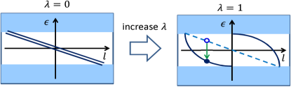
Figure 2: Schematic picture of the spectrum of a chiral $d$-wave superfluid for the smooth confinement potential (left) and sharp confinement potential (right). $\lambda$ characterizes the potential shape. Some eigenvalues changes the sign as indicated by the green arrow.

The ground state wavefunction satisfies $b^{\dagger}_{nl}|{\rm GS}(\lambda=0)\rangle=0$ when $\varepsilon_{n}(l;\lambda)<0$, while $b_{nl}|{\rm GS}(\lambda=1)\rangle=0$ when $\varepsilon_{n}(l;\lambda)>0$, where $b_{nl}$ is the $\lambda$-dependent annihilation operator of the eigen-mode of $\hat{H}_{\rm BdG}$ with $\varepsilon_{n}{(l;\lambda)}$. Let us focus on an eigenvalue $\varepsilon_{n}{(l)}$ of the first edge mode ($j=1$) which is originally positive for the smooth potential and becomes negative for the sharp potential at a critical $\lambda=\lambda_{nl}^{c}$. Because the ground state is characterized by $b_{nl}|{\rm GS}\rangle=0$ or $b_{nl}^{\dagger}|{\rm GS}\rangle=0$ depending on the sign of $\varepsilon_{n}(l)$, there will be level crossing between the ground state and an excited state at $\lambda=\lambda_{nl}^{c}$. If we denote the corresponding eigenstates as $|\Psi_{0}\rangle=|{\rm GS}\rangle$ and $|\Psi_{1}\rangle$, these two states are related as $|\Psi_{1}\rangle\sim b_{nl}^{\dagger}|\Psi_{0}\rangle$.

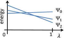
Figure 3: Schematic picture of successive level crossings between the eigenstates.

Although the fermions are fully paried up at $\lambda<\lambda_{nl}^{c}$, the Cooper pair is partially broken by the application of $b_{nl}^{\dagger}$-operator for $\lambda>\lambda_{nl}^{c}$. Once a Cooper pair of the chiral $d$-wave state which is expressed as $c_{l+2,\uparrow}^{\dagger}c_{-l,\downarrow}^{\dagger}|0\rangle$ ($|0\rangle$ is the vacuum of $c$-fermions) and carries OAM$=2$ is broken, one fermion will be removed from $|{\rm GS}\rangle$ and an unpaired single fermion mode will remain filled. By a careful analysis, it turns out that $c_{l+2,\uparrow}^{\dagger}$-fermion will remain while $c_{-l,\downarrow}^{\dagger}$-fermion is removed from the ground state where $l<-1$ in the first branch ($j=1$) of the edge modes, which reduces OAM as $(l+2)+(-l)=2\rightarrow(l+2)\leq 0$ Tada et al. (2015).

If we consider other eigenvalues, there will be a sequence of spectral flows of $\{\varepsilon_{n}(l)\}$ and corresponding successive level crossings between the eigenstates as shown in Fig. 3. Consequently, by increasing $\lambda$, the original ground state wavefunction $|{\rm GS}(\lambda=0)\rangle={\mathcal{N}}\otimes_{l}|{\rm GS}(\lambda=0),l\rangle={\mathcal{N}}\otimes_{l}\exp[\sum_{jj^{\prime}}\tilde{c}_{j,l+2,\uparrow}^{\dagger}F^{(l)}_{jj^{\prime}}\tilde{c}_{j^{\prime},-l,\downarrow}^{\dagger}]|0\rangle$ (${\mathcal{N}}$ is a normalization constant) for the smooth potential at $\lambda=0$ is replaced with the new ground state wavefunction for the sharp potential at $\lambda=1$,

$$|{\rm GS}(\lambda=1),l\rangle =\left(\prod_{j=1}^{n_{\uparrow}^{(l)}}\tilde{c}_{j,l+2,\uparrow}^{\dagger}\right)\left(\prod_{j=1}^{n_{\downarrow}^{(l)}}\tilde{c}_{j,-l,\downarrow}^{\dagger}\right)$$

$$\times\exp\left(\sum_{j>n_{\uparrow}^{(l)}}\sum_{j^{\prime}>n_{\downarrow}^{(l)}}\tilde{c}_{j,l+2,\uparrow}^{\dagger}F^{(l)}_{jj^{\prime}}\tilde{c}_{j^{\prime},-l,\downarrow}^{\dagger}\right)|0\rangle.$$ (25)

The parameters $n_{\uparrow,\downarrow}^{(l)}(\lambda),F^{(l)}_{jj^{\prime}}(\lambda)$ and the explicit form of the $\tilde{c}$-operators can be calculated from diagonalization of $\hat{H}_{\rm BdG}(\lambda)$  Tada et al. (2015); Prem et al. (2017). For $\lambda=1$, we have $(n_{\uparrow}^{(l)},n_{\downarrow}^{(l)})=(1,0)$ for $l_{1}<l<-1$, $(n_{\uparrow}^{(l)},n_{\downarrow}^{(l)})=(0,1)$ for $-1<l<l_{2}$, and $(n_{\uparrow}^{(l)},n_{\downarrow}^{(l)})=(0,0)$ otherwise, where $l_{j}=k_{Fj}R$. Note that although the number of unpaired fermions induced by the change in $V_{\rm con}$, i.e. the total number of $\{n_{\uparrow,\downarrow}^{(l)}\}_{l}$ in Eq. (25), is only $O(R)$ and their contributions to the ground state energy are negligibly small, they have large impacts on the edge mass current and consequently on OAM.

We believe that the depairing effect of the Cooper pairs and resulting reductions of edge mass currents are a universal mechanism in fermionic neutral superfluids, although we have used the very simple model as an example for an illustrative demonstration. For example, a chiral $p$-wave system can show spectral flow depending on system shapes, and the pair breaking effect works in lattice models as well where continuous rotational symmetry is absent Huang et al. (2015); Bouhon and Sigrist (2014); Tada (2018).

The above mechanism is analogous to the well known Landau criterion for bosonic superfluids where the preformed superfluid is broken once a bosonic excitation energy $\varepsilon(\lambda)$ becomes negative as some parameter is varied, leading to a new condensation of this boson mode. Similarly, in the present fermion case, the Cooper pair is broken once its excitation energy becomes negative, and the resulting ground state is a state with broken Cooper pairs, i.e. unpaired fermions. The essential difference is that Cooper pairs are broken only for the modes with sign changing eigenvalues in the fermion case. We call this partial breaking of fermion superfluidity as “fermionic Landau criterion”. The similarity between the fermionic Landau criterion and bosonic Landau criterion will be discussed in detail in the next section. It should be noted that the fermionic Landau criterion is based on a given mean field Hamiltonian where the gap function is simply given and therefore it does not necessarily hold in general interacting models. In a realistic interacting model, it may be possible that the system goes into a completely different phase as the parameter $\lambda$ is varied, if the energy cost due to unpaired fermions is $O(V)$.

III.2 Superfluid under uniform linear flow

In this section, we study a toy model for a superfluid under a uniform linear flow Tinkham (2004); Bardeen (1962) to clarify the analogy between the fermionic Landau criterion and well-known bosonic Landau criterion. This analogy is helpful to understand the physics in a comprehensive way.

We consider a non-interacting $s$-wave superfluid with a modulating gap function $\Delta_{0}\exp(i\mbox{\boldmath$q$}\mbox{\boldmath$r$})$ under periodic boundary conditions,

$${H}_{\rm FF} =\sum_{k\sigma}\varepsilon_{k}c^{\dagger}_{k\sigma}c_{k\sigma}+\sum_{k}\Delta_{0}c^{\dagger}_{k+q\uparrow}c^{\dagger}_{-k\downarrow}+{\rm(h.c.)}$$

$$=\sum_{k}\left[\begin{array}[]{c}c^{\dagger}_{k+q\uparrow}\\ c_{-k\downarrow}\end{array}\right]^{T}\left[\begin{array}[]{cc}\varepsilon_{k+q}&\Delta_{0}\\ \Delta_{0}&-\varepsilon_{-k}\end{array}\right]\left[\begin{array}[]{c}c_{k+q\uparrow}\\ c^{\dagger}_{-k\downarrow}\end{array}\right]$$ (32)

where $\varepsilon_{k}=k^{2}/2m-\mu$. The Hamiltonian has a conserved quantity

$${\mbox{\boldmath$\mathcal{P}$}}={\mbox{\boldmath$P$}}-\mbox{\boldmath$q$}{N}/2,$$ (33)

where ${N}=\sum_{k\sigma}c_{k\sigma}^{\dagger}c_{k\sigma}$ and $P$ is the total linear momentum ${\mbox{\boldmath$P$}}=\sum_{k\sigma}\mbox{\boldmath$k$}c_{k\sigma}^{\dagger}c_{k\sigma}$. This momentum $\mathcal{P}$ characterizes the deviation from the naively expected value $\langle\mbox{\boldmath$P$}\rangle_{V}=\mbox{\boldmath$q$}\langle N\rangle_{V}/2$. Eigenvalues of the BdG Hamiltonian $H_{k}$ are

$$E_{k1,2} =\frac{1}{2}\Bigl{[}\varepsilon_{k+q}-\varepsilon_{-k}\pm\sqrt{(\varepsilon_{k+q}+\varepsilon_{-k})^{2}+4\Delta_{0}^{2}}\Bigr{]}.$$ (34)

$E_{ki}$ vanishes when $|\varepsilon_{k+q}-\varepsilon_{-k}|=\sqrt{(\varepsilon_{k+q}+\varepsilon_{-k})^{2}+4\Delta_{0}^{2}}$ or equivalently $\varepsilon_{k+q}\varepsilon_{-k}+4\Delta_{0}^{2}=0$ which can be satisfied only in the BCS regime $\mu>0$. The momentum space is divided into three regions depending on signs of the eigenvalues, $K_{1}=\{\mbox{\boldmath$k$}|E_{k1}<0,E_{k2}<0\}$, $K_{2}=\{\mbox{\boldmath$k$}|E_{k1}>0,E_{k2}>0\}$, and $K_{3}=\{\mbox{\boldmath$k$}|E_{k1}>0,E_{k2}<0\}$ as shown in Fig. 4. Note that the volumes of $K_{1,2}$ are the same by the particle-hole symmetry.

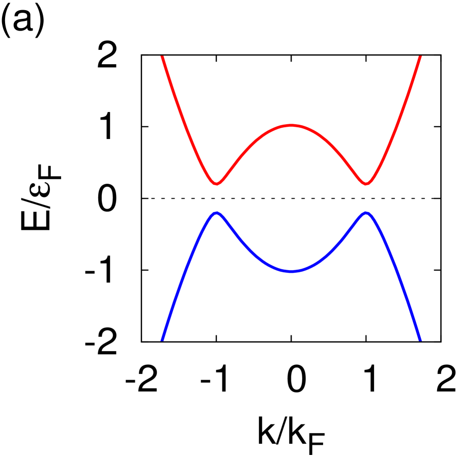
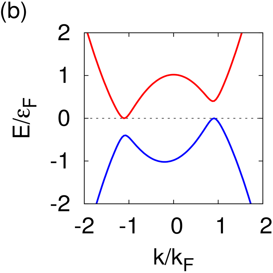
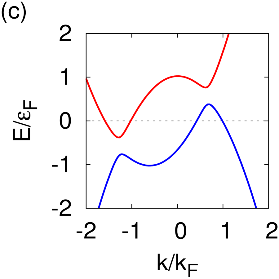
Figure 4: Dispersions in the BCS states in one-dimension at $\mu=\varepsilon_{F},\Delta_{0}=0.2\varepsilon_{F}$ for (a) $v_{s}=0$, (b) $v_{s}=v_{L}$, and (c) $v_{s}=3v_{L}$, where $v_{s}=|\mbox{\boldmath$q$}|/2m_{0}$ and $v_{L}=\Delta_{0}/k_{F}$. (d) Dispersion in the BEC state at $\mu=-0.3\varepsilon_{F},\Delta_{0}=0.2\varepsilon_{F},v_{s}=v_{L}$. Red curve is $E_{k1}$ and blue curve is $E_{k2}.$

Then, the ground state wavefunction determined by the conditions $b_{ki}|{\rm GS}\rangle=0(E_{ki}>0)$ and $b_{ki}^{\dagger}|{\rm GS}\rangle=0(E_{ki}<0)$, and is given by

$$|{\rm GS}\rangle ={\mathcal{N}}\left(\prod_{k\in K_{1}}c^{\dagger}_{k+q\uparrow}\right)\left(\prod_{k\in K_{2}}c^{\dagger}_{-k\downarrow}\right)$$

$$\quad\times\prod_{k\in K_{3}}\exp\left(-v_{k}/u_{k}c^{\dagger}_{k+q\uparrow}c^{\dagger}_{-k\downarrow}\right)|0\rangle,$$ (35)

where $(u_{k},v_{k})^{T}$ are eigenvectors of the Bogoliubov-de Gennes equation and ${\mathcal{N}}$ is a normalization constant. One can find an essential similarity between Eqs. (35) and (25). Note that, for example when $q_{x}>0$, $k_{x}+q_{x}<0$ for $\mbox{\boldmath$k$}\in K_{1}$ is satisfied, and breaking of a Cooper pair $c_{k+q\uparrow}^{\dagger}c_{-k\downarrow}^{\dagger}|0\rangle\rightarrow c_{k+q\uparrow}^{\dagger}|0\rangle$ will reduce the linear momentum as $(k_{x}+q_{x})+(-k_{x})=q_{x}>0\rightarrow(k_{x}+q_{x})<0$ as in the OAM of neutral superfluids discussed in the previous section. Similar reduction of the linear momentum takes place for $\mbox{\boldmath$k$}\in K_{2}.$

The reduction of the linear momentum can be clearly discussed based on the unpaired fermions and fermionic Landau criterion. The expectation value of the momentum deviation is $\langle{\rm GS}|{\mbox{\boldmath$\mathcal{P}$}}|{\rm GS}\rangle=-1/2\sum_{k}(\mbox{\boldmath$k$}+\mbox{\boldmath$q$}/2)\sum_{i}{\rm sgn}E_{ki}$, or equivalently,

$$\langle\mbox{\boldmath$P$}\rangle_{V} =\mbox{\boldmath$q$}\frac{\langle N\rangle_{V}}{2}-\frac{1}{2}\sum_{k}(\mbox{\boldmath$k$}+\mbox{\boldmath$q$}/2)\eta_{k},$$ (36)

$$\eta_{k} =\sum_{i=1,2}{\rm sgn}E_{ki}.$$ (37)

If the supercurrent velocity $v_{s}=|\mbox{\boldmath$q$}|/2m_{0}$ is smaller than the Landau critical velocity $v_{L}=\Delta_{0}/k_{F}$, $K_{1,2}$ are empty and functional structure of $|{\rm GS}\rangle$ is essentially same as that of the conventional full gap BCS state and $\langle\mbox{\boldmath$\mathcal{P}$}\rangle_{V}=0$, i.e. $\langle\mbox{\boldmath$P$}\rangle_{V}=\mbox{\boldmath$q$}\langle N\rangle_{V}/2$. On the other hand, when the supercurrent velocity is sufficiently fast, $v_{s}\gtrsim v_{L}$, the two regions $K_{1,2}$ are non-empty, leading to $|\langle\mbox{\boldmath$P$}\rangle_{V}|<|\mbox{\boldmath$q$}|\langle N\rangle_{V}/2$ in the BCS regime where $\mu>0$. The ground state now contains a non-zero fraction of normal state fermions, i.e. unpaired fermions, and the system has both a Fermi surface and Cooper pairs. This means that, the fast flow causes depairing of the Cooper pairs for the fermions with $|\varepsilon_{k+q}-\varepsilon_{-k}|\gtrsim 2\Delta_{0}$. Therefore, the present toy model is quite analogous to the original setup of the bosonic Landau criterion. It is noted that, in contrast to the BCS regime with $\mu>0$, $K_{1,2}$ are always empty and $\langle\mbox{\boldmath$P$}\rangle_{V}=\mbox{\boldmath$q$}\langle N\rangle_{V}/2$ in the BEC regime where $\mu<0$ as shown in Fig. 4 (d).

As was mentioned in the previous section, the Landau criterion does not necessarily hold in general interacting models. In an interacting model of the Fulde-Ferrell superfluid, a large $q>v_{L}$ will eventually destroy the whole superfluidity and the system will become a normal state (non-superfluid) Tinkham (2004); Bardeen (1962). To evaluate the stability of the pre-assumed gap function, we need to calculate the ground state energy or free energy of the interacting model. This is also true for other non-trivial state with unpaired fermions, such as the breached pair state where gapless modes with a Fermi surface coexist with paired fermions Liu and Wilczek (2003); Forbes et al. (2005).

IV iDMRG calculation of mass current

In the previous section, we have established the physical picture of the fragile spontaneous OAM in neutral fermionic superfluids based on the mean field approximation. A natural question is that whether or not the physics within the mean field description can be justified when we fully include interactions. In this section, we try to go beyond the mean field approximation by treating many-body interactions properly.

Here, we consider a model of the chiral $p$-wave superfluid with domains of opposite superfluid chiralities for an illustrative perpose. Within the mean field approximation, it is known that domain wall current is reversed depending on details of the domain boundary in such a system Tsutsumi (2014); Tada (2018); the domain wall mass current flows in a certain direction for the $(p_{x}+ip_{y})/(p_{x}-ip_{y})$ domain junction, while it is in an opposite direction for the $(p_{x}+ip_{y})/(-p_{x}+ip_{y})$ domain junction, which can be understood in terms of the unpaired fermions and fermionic Landau criterion Tada (2018). This is a drastic change in the domain wall mass current, and it would be relatively easy to discuss whether this holds true beyond the mean field approximation. It is noted that the domain wall mass current and edge mass current have essentially the same origin in common, and both of their dependences on boundaries can be understood based on the unpaired fermions and fermionic Landau criterion in the same way Tada et al. (2015); Tada (2018). Therefore we expect that studying the former is relevant to the latter.

Our Hamiltonian is a spinless fermion model with nearest neighbor attractive interaction on a two-dimensional square lattice,

$$H =\sum_{i,j}-t_{ij}c_{i}^{\dagger}c_{j}+V_{0}\sum_{\langle i,j\rangle}n_{i}n_{j}+H_{\rm SB},$$ (38)

$$H_{\rm SB} =\sum_{\langle i,j\rangle}[\Delta^{0}_{ij}c_{i}^{\dagger}c_{j}^{\dagger}+({\rm h.c.})],$$ (39)

where $t_{ij}=t(i\neq j)$ is the nearest neighbor hopping and $t_{ii}=\mu$ is the chemical potential. We have introduced a small symmetry breaking field of U(1) symmetry $\Delta^{0}_{ij}$ which describes a domain structure. Although the symmetry breaking field must be $\Delta^{0}\rightarrow 0$ after the thermodynamic limit is taken, we keep a small value of $\Delta^{0}_{ij}$ and discuss effects of the interaction $V_{0}$ in a finite size system. This calculation allows us to examine whether or not the mean field understanding is essentially correct. We apply infinite density matrix renormalization group (iDMRG) and use the open source code TenPy White (1992); Schollwöck (2005, 2011); pap (a, b); Kjäll et al. (2013). The system size is $\infty\times L_{y}$ with periodic boundary condition for the $y$-direction. To realize the domain structure shown in Fig. 5, the symmetry breaking field is taken to be $\Delta^{0}_{ij}=e^{i\theta_{i}}\Delta_{0}(\delta_{i,j+\hat{x}}\pm i\delta_{i,j+\hat{y}})$ for a site $i=(x,y)$ when $nL_{x}\leq x<(n+1)L_{x}$ and $(n+1)L_{x}\leq x<(n+2)L_{x}$ respectively, where $L_{x}$ is the domain size and $n$ is an integer.

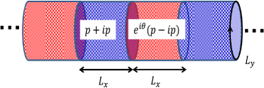
Figure 5: Infinite length cylinder with the circumference $L_{y}$. Each domain size is $L_{x}\times L_{y}$.

The phase $\theta_{i}$ characterizes the structure of a domain wall; (I) $\theta_{i}=0$ for which $\Delta_{i,j+\hat{y}}$ changes the sign at the boundary and (II) $\theta_{i}=\delta_{x,nL_{x}}\pi$ for which $\Delta_{i,j+\hat{x}}$ changes the sign. The chirality of a domain is independent of $\theta_{i}$. It is known that the domain wall corresponding to (I) is more stable than that of (II) within mean field calculations Tada (2018); Salomaa and Volovik (1989). The important point is that the directions of the domain wall currents for the two domain walls are opposite, which is rather counter-intuitive since a domain wall current in a chiral $p$-wave state is usually determined by the chirality of the gap function. This non-trivial behavior can be understood based on the unpaired fermions and fermionic Landau criterion Tada (2018). Here, we discuss validity of the physical understanding based on the mean field approximations with use of iDMRG which are essentially free from approximations White (1992); Schollwöck (2005, 2011); pap (a, b); Kjäll et al. (2013).

Now we numerically evaluate the mass current density for each domain wall, $\theta=0$ or $\theta=\pi$. We have done similar calculations for several values of the symmetry breaking field $\Delta_{0}$ and different system sizes $L_{x},L_{y}$, and they show qualitatively similar results. In the following, we focus on the smallest symmetry breaking field $\Delta_{0}=0.01t$ used in the calculations, and fix the system size as $L_{x}=L_{y}=8$. The bond dimension $\chi$ controls accuracy of the iDMRG calculations, and we used only three values $\chi=200,400,600$. Although these are not sufficient to obtain fully convergent results, they give qualitatively same results. Therefore, we fix $\chi=400$ in the following to discuss the validity of the mean field approximations, for which the truncation norm error is $O(10^{-4})$. The relatively small truncation error for the parameters used is due to the symmetry breaking field $\Delta_{0}$ which makes the bulk of the system gapped.

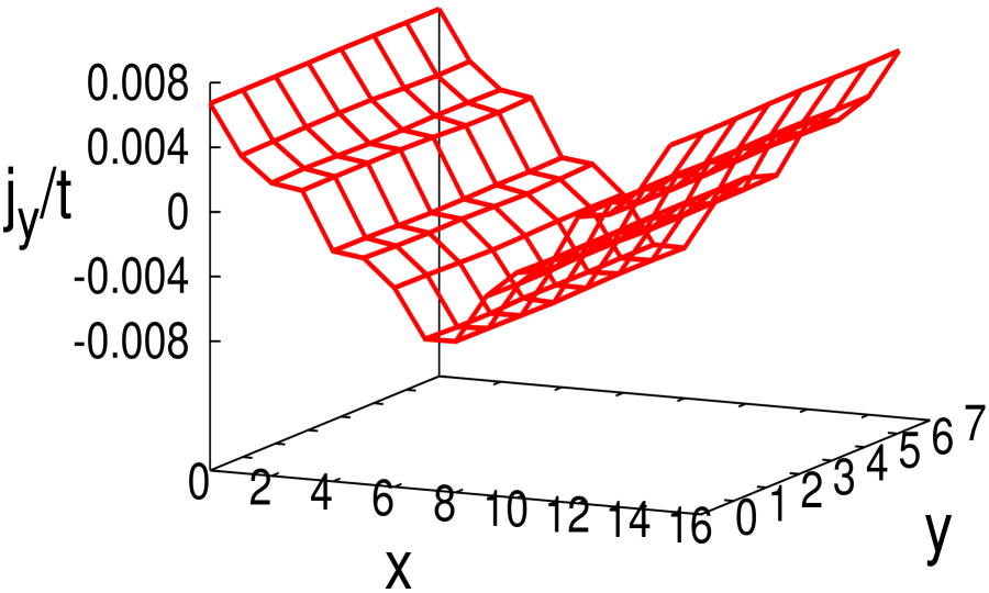
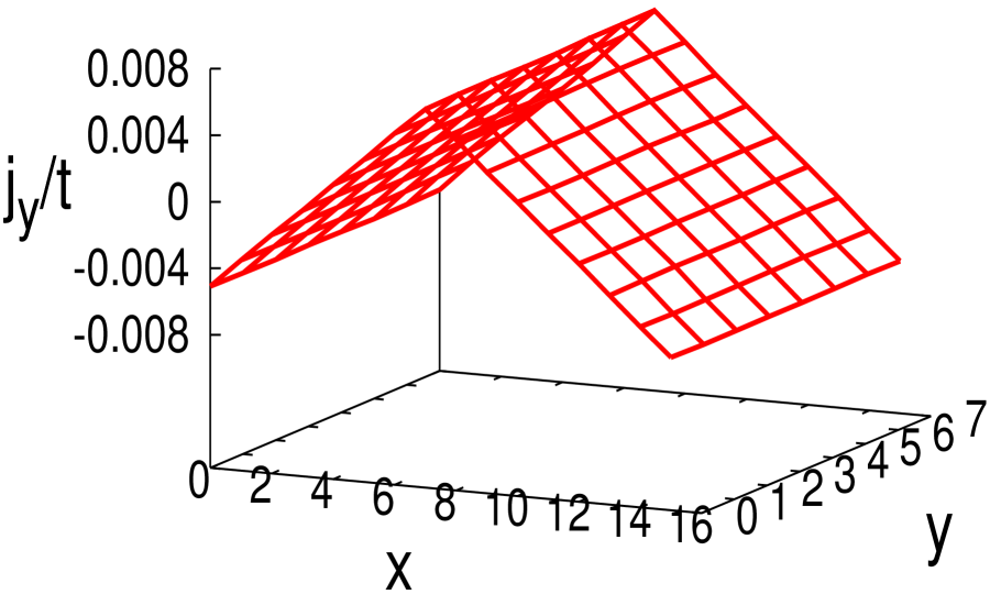
Figure 6: Mass current density along the $y$-direction for $\theta=0$ (left) and $\theta=\pi$ (right). The parameters are $V_{0}=-0.1t,\mu=-t$. The chirality of $\Delta^{0}$ is positive for $0\leq x<L_{x}=8$, while it is negative for $L_{x}\leq x<2L_{x}=16$.

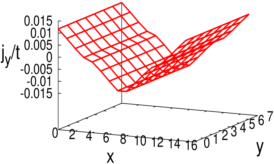
Figure 7: Mass current density along the $y$-direction for $\theta=0$ (left) and $\theta=\pi$ (right). The parameters are $V_{0}=-t,\mu=-2.2t$. The chirality of $\Delta^{0}$ is positive for $0\leq x<L_{x}=8$, while it is negative for $L_{x}\leq x<2L_{x}=16$.

We show in Fig. 6 the calculated mass current densities at a small interaction $V_{0}=-0.1t,\mu=-t$ for which the average particle filling is $n\simeq 0.32$. Unfortunately, the current profile does not show sharp localization at a domain boundary, since the system size $L_{x}=L_{y}=8$ is not large enough compared with the coherence length for the parameters used. Instead, the current profile shows a broad structure where $|j_{y}|$ is largest at the domain boundary, while it is smallest in the middle of a domain. Nevertheless, the current directions for $\theta=0$ and $\theta=\pi$ are opposite, which is consistent with the mean field calculations Tsutsumi (2014); Tada (2018). The ground state energy difference between the two states is small, $[E(\theta=0)-E(\theta=\pi)]/[E(\theta=0)+E(\theta=\pi)]=O(10^{-3})$. Now we increase the interaction and find that the current reversal is stable even for a relatively large interaction $V_{0}=-t,\mu=-2.2t$ for which $n\simeq 0.28$, as shown in Fig. 7. The mass current is enhanced by the interaction $V_{0}$ and the maximum density becomes nearly double compared with those for $V_{0}=-0.1t$ if $j_{y}$ is normalized by the filling $n$. This means that $j_{y}$ is dominated by the interaction $V_{0}=-t$ and the current reversal gets stabilized. The origin of the enhancement of $j_{y}$ would be the decreased superfluid coherence length $\xi_{\Delta}\simeq t/\Delta$ by the interaction $V_{0}$ where $\Delta$ is the gap amplitude, because a small $\xi_{\Delta}$ gives $j_{y}$ which is well localized around a boundary and does not influence $j_{y}$ at the opposite boundary. If we increase $|V_{0}|$ further, the simulations become unstable and the fermions get dimerized. These numerical results suggest that the current reversal found in the mean field calculations holds true even in the iDMRG calculations which are essentially free from approximations. Therefore, we conclude that the physical understanding based on the mean field approximation is essentially correct, and the physics is determined by the unpaired fermions and fermionic Landau criterion. Finally, although our iDMRG results support the correctness of the mean field understanding, they are reliable at a rather qualitative level and further numerical calculations would be required to develop a quantitative understanding.

V summary and discussion

In this study, we have discussed the OAM and corresponding edge or domain wall mass current in neutral fermion superfluids with broken time reversal symmetry. It was explained that OAM in a neutral superfluid cannot be obtained by derivative of the thermodynamic free energy with respect to its intensive conjugate external field in sharp contrast to non-superfluid systems. This means that OAM in a neutral superfluid is not a thermodynamic quantity and can be influenced by non-thermodynamic details. We established a simple physical picture of how OAM is changed by such perturbations based on the mean field approximation, by introducing the concepts of the unpaired fermions and fermionic Landau criterion. We also discussed the validity of the mean field description by a non-perturbative numerical calculation using iDMRG. It is concluded that the mean field calculations of OAM and edge mass current for chiral superfluids are essentially correct, and OAM does depend on non-thermodynamic details such as boundary conditions which are usually not controlable in experiments. The sensitivity of OAM can be considered as an anomalously colossal response of OAM to boundaries. If one could control the boundary conditions of a neutral superfluid, a dramatic response of OAM by small perturbations might be obtained.

In the original problem of the “intrinsic angular momentum paradox” in ³He-A phase in three dimensions, the rotation axis of Cooper pairs will locally deviates near the wall of a container from that in the bulk Vollhart and Wölfle (1990); Volovik (2003); Leggett (1975, 2006, 2012); Mizushima et al. (2016). Because this effect may depend on the container used, some people have anticipated that this problem would depend on theoretical models used and experimental details. However, such a subtle problem is absent in simpler systems such as the thin film limit of a chiral $p$-wave state and two-,three-dimensional chiral $d$-wave state, and one may expect an “intrinsic” value of the spontaneous OAM. What we have discussed in this study is that, even in such a relatively simple system, there is no “intrinsic” value of OAM in a uniform neutral superfluid, simply because it is not a thermodynamic quantity.

The OAM and edge mass current of a neutral superfluid will be determined for each given surface condition and sample shape. There exist various possible perturbations such as surface adsorption, surface reconstruction, and surface disorder, and surface conditions should be carefully treated in experiments, although it is a very difficult issue. Sample shapes and relative relations between the surface direction and underlying lattice geometry should also be controlled in solid state superconductors, to observe edge charge currents.

Finally, we touch on charged chiral superconductors such as the candidate $p$-wave superconductor Sr₂RuO₄. It is considered that the edge current depends on boundaries in this system Hicks et al. (2010); Scaffidi and Simon (2015). In such a system, there arises a Meissner screening current in addition to a spontaneous edge current. The former is localized at a surface in the length scale of coherence length, while the latter is in the length scale of penetration depth, and they are spatially separated. These two contributions will cancel each other in a longer length scale, and the total net edge current $\mbox{\boldmath$J$}_{\rm edge}$ and corresponding spontaneous OM vanishes in absence of an external field Tada (2018). Since the spontaneous edge current which we have discussed in the present study depends on boundaries and shapes of the system, the corresponding screening current also depends on them. Therefore, the induced local magnetic flux density which is to be measured in experiments would also be sensitive to boundaries and shapes.

Appendix A Thermodynamic limit under uniform flux density

We explain that the thermodynamic limit exists for a U(1) symmetric system with a given uniform magnetic flux density. The existence proof is the same as in the previous studies, once one notices that the Hamiltonian is stable and translationally symmetric with an appropriate gauge transformation Ruelle (1999). Nevertheless, as a reference, here we will give a brief discussion on both lattice models and continuum models with stable, short-range interactions. It should be noted that existence of a thermodynamic limit for a system with long-range interactions is highly non-trivial, and for example, one would find the familiar shape/boundary condition dependent free energy density of a magnet with dipole interactions in the presence of an external field  Banerjee et al. (1998); Campa et al. (2009). Long range interactions or dynamics of electromagnetic field is beyond the present study. We also discuss Bloch’s theorem on absence of a macroscopic current at equilibrium as a collorary of the existence of the thermodynamic limit.

A.1 Lattice model

We consider a simple model defined on a lattice $\Lambda\subset{\mathbb{Z}}^{d}$ where $d=3$ is the system dimension,

$$H_{\Lambda} =\sum_{i,j}-t_{ij}c_{i}^{\dagger}c_{j}+V\sum_{\langle i,j\rangle}n_{i}n_{j},$$

$$\equiv\sum_{X\subset\Lambda}h_{X},$$ (40)

where $X=\{i\},\langle i,j\rangle$ represents sites or nearest neighbor pairs of sites. The hopping term contains a given vector potential $A_{ij}$ which realizes a uniform magnetic flux density along $z$-axis, and its amplitude $|t_{ij}|$ is constant. We have also included the chemical potential, $t_{ii}=\mu$. It is important to see that the Hamiltonian is symmetric under the magnetic translation. We denote the $n_{\mu}$-sites magnetic translation operator along $\mu$-direction as $T_{\mu}(n_{\mu})$. Then, for a translation $T(n)=T_{x}(n_{x})T_{y}(n_{y})T_{z}(n_{z})$,

$$H_{\Lambda+n}=T(n)H_{\Lambda}T(n)^{-1},$$ (41)

where $\Lambda+n$ is the translate of $\Lambda$ by the vector $n$. This relation is independent of the order of $T_{x},T_{y},T_{z}$ in $T$, since they are a projective representation of translation. Therefore, the free energy density $f_{\Lambda}=F_{\Lambda}/|\Lambda|$ is also translationally symmetric

$$f_{\Lambda+n}=f_{\Lambda}.$$ (42)

For simplicity, we consider a cube $\Lambda_{a}=\{x\in{\mathbb{Z}}^{d}|0\leq x_{\mu}<a\}$ and a larger cube $\Lambda=\{x\in{\mathbb{Z}}^{d}|0\leq x_{\mu}<la\}$ where $l,a$ are positive integers. We define $\Lambda_{a+n}=\{x\in{\mathbb{Z}}^{d}|n_{\mu}a\leq x_{\mu}<(n_{\mu}+1)a\}$ and denote them as $\{\Lambda_{j}\}_{j=1}^{l^{d}}$ so that $\Lambda=\cup_{j=1}^{l^{d}}\Lambda_{j}$.

We compare the free energy densities $f_{\Lambda}$ and $f_{\Lambda_{a}}$. For $\Gamma_{j}=\cup_{i=1}^{j}\Lambda_{i}$, one can show

$$|F_{\Lambda}-\sum_{j=1}^{l^{d}}F_{\Lambda_{j}}|\leq||h||\sum_{j=2}^{l^{d}}N(\Gamma_{j-1},\Lambda_{j}),$$ (43)

where $N(\Gamma_{j-1},\Lambda_{j})$ is the number of sites for which $h_{\langle k,l\rangle}\neq 0$ with $k\in\Gamma_{j-1}$ and $l\in\Lambda_{j}$. We have introduced $||h||=\sum_{X\ni 0}||h_{X}||/|X|$ which is well defined because $h_{X}$ is magnetic translationally symmetric. It is important to see that the seemingly dangerous terms in $h_{X}$ close to the boundary of $\Lambda_{j}$ are harmless in the presence of the vector potential. Since $N(\Gamma_{j-1},\Lambda_{j})=O(a^{2})$ for large $a$, we have

$$|f_{\Lambda}-f_{\Lambda_{a}}|=O(1/a),$$ (44)

which means the existence of the thermodynamic limit $f_{\infty}=\lim_{\Lambda\rightarrow{\mathbb{Z}}^{d}}f_{\Lambda}$. One can also show the existence of the thermodynamic limit for a more general sequence of lattices, and the resulting $f_{\infty}$ is independent of the system shape for such lattices.

A.2 Continuum model

We next touch on continuum models. Although discussions on continuum models are generally complicated, the proof for Hamiltonian with usual translation symmetry can also be applied to that with magnetic translational symmetry Ruelle (1999).

We consider a Hamiltonian of $N$ fermions,

$$H_{\Lambda,N} =T_{\Lambda,N}+U_{\Lambda,N},$$ (45)

$$T_{\Lambda,N} =\sum_{j=1}^{N}\frac{1}{2m}\bigl{(}-i\nabla_{j}-\mbox{\boldmath$A$}(\mbox{\boldmath$r$}_{j})\bigr{)}^{2},$$ (46)

$$U_{\Lambda,N} =\sum_{i<j}U(|\mbox{\boldmath$x$}_{i}-\mbox{\boldmath$x$}_{j}|),$$ (47)

where the vector potential gives a constant magnetic flux density. The interaction is stable ($U_{\Lambda,N}>-bN$ with $b\geq 0$) and short-range with the range $r_{0}$ or strongly tempered, $U(r>r_{0})\leq 0$. $\Lambda\subset{\mathbb{R}}^{d}$ is a bounded region, and we consider wavefunctions which smoothly tend to zero at the boundary $\partial\Lambda$ and vanishes outside of $\Lambda$. Mathematically, $H_{\Lambda,N}$ should be regarded as a self-adjoint Friedrichs extension.

The spectrum of $H_{\Lambda,N}$ consists of discrete eigenvalues with finite multiplicity, and we denote them in increasing order as $E_{1}\leq E_{2}\leq\cdots$. Then, the minimax principle reads

$$E_{m}=\inf_{{\mathcal{M}}:{\rm dim}{\mathcal{M}}=m}\sup_{\phi:\phi\in{\mathcal{M}},||\phi||=1}\langle\phi|H|\phi\rangle.$$ (48)

Now we discuss entropy $S_{\Lambda}(N,E)=\log W_{\Lambda}(N,E)$, where $W_{\Lambda}(N,E)$ is the number of eigenvalues of $H_{\Lambda,N}$ below $E$. Note that $S_{\Lambda}$ is translationally invariant, since the Hamiltonian has magnetic translational symmetry. We consider two regions $\Lambda_{i}(i=1,2)$ which are separated by the distance $r\geq r_{0}$, and $N_{i}$ particles are confined in each region, respectively. The states with energy of $H_{\Lambda_{i},N_{i}}$ below $E_{i}$ are described by wave functions $\varphi_{i}\in{\mathcal{M}}_{i}$ which satisfy the hard wall boundary condition $\varphi_{i}(x\in\partial\Lambda_{i}^{N_{i}})=0$, for which dim${\mathcal{M}}_{i}=\Omega_{\Lambda_{i}}(N_{i},E_{i})$. From the minimax principle, we have

$$\sup_{\varphi_{i}\in{\mathcal{M}}_{i},||\varphi_{i}||=1}\langle\varphi_{i}|H_{\Lambda_{i},N_{i}}|\varphi_{i}\rangle\leq E_{i}.$$ (49)

Now we construct a subspace ${\mathcal{M}}_{1+2}$ of the total Hilbert space for particles in $\Lambda_{1}\cup\Lambda_{2}$; ${\mathcal{M}}_{1+2}$ is generated by antisymmetrized $\varphi_{1}\otimes\varphi_{2}$ and its dimension is dim${\mathcal{M}}_{1+2}=\Omega_{\Lambda_{1}}(N_{1},E_{1})\cdot\Omega_{\Lambda_{2}}(N_{2},E_{2}).$ Note that $\varphi\in{\mathcal{M}}_{1+2}$ vanishes on $(\partial\Lambda_{1})\cup\Lambda_{2}$ or $\Lambda_{1}\cup(\partial\Lambda_{2})$, and seemingly dangerous contributions to $\Omega_{\Lambda_{1}\cup\Lambda_{2}}(N_{1}+N_{2},E)$ from those boundaries are harmless in the presence of the vector potential $|\mbox{\boldmath$A$}|\propto|\mbox{\boldmath$r$}|$, as in lattice models. Since $\sup_{\varphi\in{\mathcal{M}}_{1+2},||\varphi||=1}\langle\varphi|H_{\Lambda_{1}\cup\Lambda_{2},N_{1}+N_{2}}|\varphi\rangle\leq E_{1}+E_{2}$, we obtain

$$S_{\Lambda_{1}\cup\Lambda_{2}}(N_{1}+N_{2},E_{1}+E_{2})\geq S_{\Lambda_{1}}(N_{1},E_{1})+S_{\Lambda_{2}}(N_{2},E_{2}).$$ (50)

Furthermore, $S_{\Lambda}$ is an increasing function of $\Lambda$, i.e. $S_{\Lambda}\leq S_{\Lambda^{\prime}}$ if $\Lambda\subset\Lambda^{\prime}$. Therefore, for a sequence of regions $\Lambda_{j}=\{x\in{\mathbb{R}}^{d}|0\leq x\leq L_{j}=2L_{j-1}+r_{0}\}$ such that $\Lambda_{j}$ contains $2^{d}$ translates of $\Lambda_{j-1}$ with mutual distance $r_{0}$, $s_{\Lambda_{j}}=S_{\Lambda_{j}}(N_{j},E_{j})/|\Lambda_{j}|$ with $N_{j}=2^{d}N_{j-1},E_{j}=2^{d}E_{j-1}$ is a non-decreasing sequence. Besides, entropy of the interacting model is bounded above by that of the corresponding non-interacting model,

$$S_{\Lambda}(N,E)\leq S_{\Lambda}^{(0)}(N,E+bN),$$ (51)

since $E_{m}\geq E_{m}^{(0)}-bN$ holds, where $E_{m}^{(0)}$ is the $m$-th eigenvalue of $T_{\Lambda,N}$. Therefore, there exists the thermodynamic limit of the entropy density, $s_{\infty}=\lim_{\Lambda\rightarrow{\mathbb{R}}^{d}}s_{\Lambda}$. Because of the equivalence between different emsembles, thermodynamic limit of the free energy density also exists.

A.3 Bloch’s theorem

We briefly discuss Bloch’s theorem as a collorary of the existence of the thermodynamic limit of a U(1) symmetric system. The theorem claims that a macroscopic current is not allowed at equilibrium Tada and Koma (2016). For simplicity, we consider a Hamiltonian $H$ of fermions with short-range interactions defined on a two-dimensional cylinder $\Lambda=S_{R}\times I$ where $S_{R}$ is a one-dimensional ring with radius $R$ and $I$ is an interval, under an external field $B_{z}$ perpendicular to $S_{R}$. There might possibly arise a uniform current density $\langle\mbox{\boldmath$j$}(\mbox{\boldmath$r$}\in\Lambda)\rangle=O(1)$ around the cylinder. However, such a current density is not allowed, since if it exists, the free energy will be superextensive, $|F_{\Lambda}(B_{z}\neq 0)|=O(R^{2}\times|I|)\gg O(|\Lambda|)$ due to the coupling between $B_{z}$ and OM. Therefore, there is no net current in $\Lambda$, which is a variant of Bloch’s theorem.

The above argument has a trivial but important physical implication. Now we consider a three-dimensional ferromagnet which is fully wrapped with a thin film under the assumption that long range magnetic interactions are negligible. The total system is a combination of the decoupled ferromagnet and thin film, and the latter is described as a two-dimensional system such as the cylinder in the above discussion. Then, from the similar argument, we conclude that it is impossible to change the value of OM of the ferromagnet by wrapping it with a thin film, which sounds rather trivial. We can screen OM only when we use a superconducting thin film, where the Maxwell equation or long range magnetic interactions should be taken into account. One can compare this with the electric polarization for which a constant electric field is not a conjugate intensive field Avron and Herbst (1977); Blanc and Monneau (2002). Corresponding to the above argument, one can wrap a three-dimensional ferroelectric material by a two-dimensional metallic film, which can be regarded as a surface perturbation to the former. Obviously, the polarization of the total system, i.e. the perturbed ferroelectric material, changes due to a screening effect by the thin metal. In sharp contrast to OAM/OM, the charge polarization can be easily affected by surface perturbations even in a theoretical model with short range interactions.

Appendix B Numerical calculation of OAM

We breifly discuss numerical calculations of the OAM for the Hamiltonians Eq. (16) with the sharp confinement potential, $V(r<R)=0,V(r>R)=\infty$. The calculation results are shown in Fig. 8.

Figure 8: OAM for the Hamiltonian Eq. (16). $\Delta_{0}$ dependence for different system sizes (left panel), and global $\Delta_{0}$ dependence for the fixed system size $k_{F}R=80$ (right panel).

The OAM per fermion is nearly zero for small $\Delta_{0}/\varepsilon_{F}$, although it is slightly oscillating around zero because of finite size effects. The vanishing OAM is consistent with the semi-classical discussions given in the main text. As $\Delta_{0}$ increases, the OAM changes discretely since the spectral asymmetry $\eta_{l}$ is an integer and the total number of fermions $\langle N\rangle_{V}$ is kept constant for each system size $k_{F}R$ with the same average density (see Eq. (23)). For large $\Delta_{0}$, the system enters the strong coupling BEC regime and the OAM takes the saturated value $\langle L_{z}\rangle_{V}/\langle N\rangle_{V}=1$ Tada et al. (2015).

References

- Vollhart and Wölfle (1990) D. Vollhart and P. Wölfle, The Superfluid Phase of Helium 3, 1st ed. (Taylor and Francis, London, 1990).
- Volovik (2003) G. E. Volovik, The Universe in a Helium Droplet (Oxford University Press, Oxford, 2003).
- Leggett (1975) A. J. Leggett, Rev. Mod. Phys. 47, 331 (1975).
- Leggett (2006) A. J. Leggett, Quantum Liquids: Bose Condensation and Cooper Pairing in Condensed-matter Systems (Oxford University Press, Oxford, 2006).
- Leggett (2012) A. J. Leggett, Bussei Kenkyu 1, 0112011 (2012).
- Mizushima et al. (2016) T. Mizushima, Y. Tsutsumi, T. Kawakami, M. Sato, M. Ichioka, and K. Machida, J. Phys. Soc. Jpn. 85, 022001 (2016).
- Ishikawa (1977) M. Ishikawa, Prog. Theor. Phys. 57, 1836 (1977).
- Ishikawa et al. (1980) M. Ishikawa, K. Miyake, and T. Usui, Prog. Theor. Phys. 63, 1083 (1980).
- McClure and Takagi (1979) M. G. McClure and S. Takagi, Phys. Rev. Lett. 43, 596 (1979).
- Mermin (1977) N. D. Mermin, Physica B 90, 1 (1977).
- Mermin and Muzikar (1980) N. D. Mermin and P. Muzikar, Phys. Rev. B 21, 980 (1980).
- Volovik (1995) G. E. Volovik, JETP Lett. 61, 958 (1995).
- Kita (1996) T. Kita, J. Phys. Soc. Jpn. 65, 664 (1996).
- Kita (1998) T. Kita, J. Phys. Soc. Jpn. 67, 216 (1998).
- Goryo (1998) J. Goryo, Phys. Lett. A 246, 549 (1998).
- Anderson and Morel (1961) P. Anderson and P. Morel, Phys. Rev. 123, 1911 (1961).
- Volovik (1975) G. E. Volovik, JETP Lett. 22, 108 (1975).
- Volovik and Mineev (1976) G. E. Volovik and V. P. Mineev, Sov. Phys. JETP 44, 591 (1976).
- Cross (1975) M. Cross, J. Low Temp. Phys. 21, 525 (1975).
- Cross (1977) M. Cross, J. Low Temp. Phys. 26, 165 (1977).
- Combescot (1978) R. Combescot, Phys. Rev. B 18, 6071 (1978).
- Leggett and Takagi (1978) A. J. Leggett and S. Takagi, Ann. Phys. 110, 353 (1978).
- Hall (1985) H. E. Hall, Phys. Rev. Lett. 54, 205 (1985).
- Liu (1985) M. Liu, Phys. Rev. Lett. 55, 441 (1985).
- Stone and Anduaga (2008) M. Stone and I. Anduaga, Ann. Phys. 323, 2 (2008).
- Sauls (2011) J. A. Sauls, Phys. Rev. B 84, 214509 (2011).
- Huang et al. (2014) W. Huang, E. Taylor, and C. Kallin, Phys. Rev. B 90, 224519 (2014).
- Huang et al. (2015) W. Huang, S. Lederer, E. Taylor, and C. Kallin, Phys. Rev. B 91, 094507 (2015).
- Tada et al. (2015) Y. Tada, W. Nie, and M. Oshikawa, Phys. Rev. Lett. 114, 195301 (2015).
- Volovik (2015) G. E. Volovik, JETP Letters 100, 742 (2015).
- Ojanen (2016) T. Ojanen, Phys. Rev. B 93, 174505 (2016).
- Scaffidi and Simon (2015) T. Scaffidi and S. H. Simon, Phys. Rev. Lett. 115, 087003 (2015).
- Tsuruta et al. (2015) A. Tsuruta, S. Yukawa, and K. Miyake, J. Phys. Soc. Jpn. 84, 094712 (2015).
- Suzuki and Asano (2016) S. I. Suzuki and Y. Asano, Phys. Rev. B 94, 155302 (2016).
- Nomura et al. (2012) K. Nomura, S. Ryu, A. Furusaki, and N. Nagaosa, Phys. Rev. Lett. 108, 026802 (2012).
- Gromov and Abanov (2015) A. Gromov and A. G. Abanov, Phys. Rev. Lett. 114, 016802 (2015).
- Read (2009) N. Read, Phys. Rev. B 79, 045308 (2009).
- Read and Rezayi (2011) N. Read and E. H. Rezayi, Phys. Rev. B 84, 085316 (2011).
- Bradlyn et al. (2012) B. Bradlyn, M. Goldstein, and N. Read, Phys. Rev. B 86, 245309 (2012).
- Hoyos et al. (2014) C. Hoyos, S. Moroz, and D. T. Son, Phys. Rev. B 89, 174507 (2014).
- Shitade and Kimura (2014) A. Shitade and T. Kimura, Phys. Rev. B 90, 134510 (2014).
- Tada (2015) Y. Tada, Phys. Rev. B 92, 104502 (2015).
- Nagato et al. (2011) Y. Nagato, S. Higashitani, and K. Nagai, J. Phys. Soc. Jpn. 80, 113706 (2011).
- Lederer et al. (2014) S. Lederer, W. Huang, E. Taylor, S. Raghu, and C. Kallin, Phys. Rev. B 90, 134521 (2014).
- Bouhon and Sigrist (2014) A. Bouhon and M. Sigrist, Phys. Rev. B 90, 220511(R) (2014).
- Landau and Lifshitz (1984) L. D. Landau and E. M. Lifshitz, Statistical Physics, 3rd ed. (Butterworth-Heinemann, 1984).
- Tsutsumi (2014) Y. Tsutsumi, J. Low Temp. Phys. 175, 51 (2014).
- Tada (2018) Y. Tada, Phys. Rev. B 97, 014519 (2018).
- com (a) OM operator is defined as for a finite system with an open boundary condition, where is the gauge invariant charge current density given by the sum of the paramagnetic and diamagnetic currents. Since it is gauge invariant, we can choose for zero magnetic flux density . In this particular gauge, holds as an operator identity in finite volume systems.
- com (b) Here, we do not take dynamics of the electromagnetic field into account and is simply a given constant. The real (classical) electromagnetic field inside a sample under a given external constant is determined by the Maxwell equation, or equivalently there arises the long range Breit interaction, which makes the problem complicated. For a discussion on the long range dipole interaction, see Ref. Banerjee et al. (1998).
- Banerjee et al. (1998) S. Banerjee, R. B. Griffiths, and M. Widom, J. Stat. Phys. 93, 141 (1998).
- Angetescu et al. (1975) N. Angetescu, G. Nenciu, and M. Bundaru, Commun. Math. Phys. 42, 9 (1975).
- Macris et al. (1988) N. Macris, P. A. Martin, and J. V. Pulé, Commun. Math. Phys. 117, 215 (1988).
- Briet et al. (2012) P. Briet, H. D. Cornean, and B. Savoie, Ann. Henri Poincaré 13, 1 (2012).
- Ruelle (1999) D. Ruelle, Statistical Mechanics: Rigorous Results (Imperial College Press and World Scientific, London, 1999).
- Lieb and Seiringer (2010) E. Lieb and R. Seiringer, The Stability of Matter in Quantum Mechanics, 1st ed. (Cambridge University Press, Cambridge, 2010).
- Manninen et al. (1996) A. J. Manninen, T. D. C. Bevan, J. B. Cook, H. Alles, J. R. Hook, and H. E. Hall, Phys. Rev. Lett. 77, 5086 (1996).
- Bevan et al. (1997) T. D. C. Bevan, A. J. Manninen, J. B. Cook, H. Alles, J. R. Hook, and H. E. Hall, J. Low Temp. Phys. 109, 423 (1997).
- (59) O. Ishikawa, in Proceedings of the International Conference on Quantum Fluids and Solids, (2012); T. Kunimatsu, H. Nema, M. Kubota, R. Ishiguro, T. Takagi, Y. Sasaki, and O. Ishikawa, in Proceedings of the 67th Annual Japanese Physical Society Meeting, (2012).
- Hicks et al. (2010) C. W. Hicks, J. R. Kirtley, T. M. Lippman, N. C. Koshnick, M. E. Huber, Y. Maeno, W. M. Yuhasz, M. B. Maple, and K. A. Moler, Phys. Rev. B 81, 214501 (2010).
- White (1992) S. R. White, Phys. Rev. Lett. 69, 2863 (1992).
- Schollwöck (2005) U. Schollwöck, Rev. Mod. Phys. 77, 259 (2005).
- Schollwöck (2011) U. Schollwöck, Ann. Phys. 326, 96 (2011).
- pap (a) I. P. McCulloch, arXiv:0804.2509.
- pap (b) J. Hauschild and F. Pollmann, arXiv:1805.00055.
- Kjäll et al. (2013) J. A. Kjäll, M. P. Zaletel, R. S. K. Mong, J. H. Bardarson, and F. Pollmann, Phys. Rev. B 87, 235106 (2013).
- com (c) Rigorously speaking, might be different from . For example, if there exists a dangerous finite size correction to such as , these two evaluations will give different results Lebowitz (1968). Note that if is non-analytic at corresponding to spontaneous symmetry breaking, should be replaced with a one-sided derivative.
- Lebowitz (1968) J. E. Lebowitz, Annu. Rev. Phys. 19, 389 (1968).
- com (d) For a perturbation , the change of the free energy is bounded as from the Peierls inequality Ruelle (1999), where is an expectation with the Hamiltonian .
- com (e) Here, we say that a bounded operator defined on is extensive when . For a unbounded operator we consider a subspace of the Hilbert space where is bounded.
- Tada and Koma (2016) Y. Tada and T. Koma, J. Stat. Phys. 165, 455 (2016).
- com (f) The net edge mass current is well-defined as long as is well-localized around the boundary of a system.
- com (g) A non-local expression of OAM density could be obtained for the expectation value of OAM in a particle U(1) symmetric system. The simplest example is where is the solution of with an additional boundary condition, where the continuity equation has been used. The OAM expectation density in metals and insulators was discussed recently Bianco and Resta (2013); Marrazzo and Resta (2016).
- Bianco and Resta (2013) R. Bianco and R. Resta, Phys. Rev. Lett. 110, 087202 (2013).
- Marrazzo and Resta (2016) A. Marrazzo and R. Resta, Phys. Rev. Lett. 116, 137201 (2016).
- Widom (1968) A. Widom, Phys. Rev. 168, 150 (1968).
- com (h) Another important exception is a system of electrons and nueclei with the Coloumb interaction under a uniform external electric field. For such a system, some electrons will escape from the nueclei and the ground state energy negatively diverge, and therefore the Hamiltonian does not have stability of the first kind when the system is placed in . Although the metastable state where all the electrons are trapped by the nueclei has a very long relaxation time, electric polarization ( is the total charge density) is not a thermodynamic quantity in a strict sense similar to OAM in a rotating system Avron and Herbst (1977); Blanc and Monneau (2002).
- Avron and Herbst (1977) J. E. Avron and I. W. Herbst, Commun. Math. Phys. 52, 239 (1977).
- Blanc and Monneau (2002) X. Blanc and R. Monneau, Adv. Differential Equations 7, 847 (2002).
- com (i) A similar condition is required in a relativistic system so that the maximum velocity at a surface does not exceed the speed of light Davies et al. (1996); Duffy and Ottewill (2003); Mameda and Yamamoto (2016).
- Davies et al. (1996) P. C. W. Davies, T. Dray, and C. A. Manogue, Phys. Rev. D 53, 4382 (1996).
- Duffy and Ottewill (2003) G. Duffy and A. C. Ottewill, Phys. Rev. D 67, 044002 (2003).
- Mameda and Yamamoto (2016) K. Mameda and A. Yamamoto, Prog. Theor. Exp. Phys. 2016, 093B05 (2016).
- Leggett (1970) A. J. Leggett, Phys. Rev. Lett. 25, 1543 (1970).
- Leggett (1998) A. J. Leggett, J. Stat. Phys. 93, 927 (1998).
- Yoshioka and Fukuyama (1992) D. Yoshioka and H. Fukuyama, J. Phys. Soc. Jpn. 61, 2368 (1992).
- com (j) The free energy density will diverge even when one introduces an oscillating magnetic flux density such as and take limit. This is trivial when we take the limit before the thermodynamic limit is taken to realize a -field which is constant over the whole system. We could also describe a nearly uniform -field by taking the limit first, and then take . In this case, for example, the induced current density will be essentially proportional to the vector potential and it would diverge as for large .
- com (k) The former would correspond to a system weakly coupled to an environment which works as a bath for the number of particles. On the other hand, the latter does to an isolated system or a system coupled to a heat bath without interchanging particles. A comparison between these two descriptions can be found, for example in Ref. Shimizu and Miyadera (2001).
- Shimizu and Miyadera (2001) A. Shimizu and T. Miyadera, Phys. Rev. E 64, 056121 (2001).
- com (l) Here, we focus on a system where the non-interacting Hamiltonian has the time-reversal symmetry. There are other models of time-reversal symmetry broken superfluids where time-reversal symmetry is already absent in the non-interacting Hamiltonian, such as Rashba spin-orbit coupled -wave superfluid with population imbalance Sato and Fujimoto (2016). For such a system, the global phase of the gap function is not important and we do not need to introduce a U(1) symmetry breaking field. Correspondingly, is also evaluated as in the scheme (ii).
- Sato and Fujimoto (2016) M. Sato and S. Fujimoto, J. Phys. Soc. Jpn. 85, 072001 (2016).
- Prem et al. (2017) A. Prem, S. Moroz, V. Gurarie, and L. Radzihovsky, Phys. Rev. Lett. 119, 067003 (2017).
- Tinkham (2004) M. Tinkham, Introduction to Superconductivity (Dover Publications, New York, 2004).
- Bardeen (1962) J. Bardeen, Rev. Mod. Phys. 34, 667 (1962).
- Liu and Wilczek (2003) W. V. Liu and F. Wilczek, Phys. Rev. Lett. 90, 047002 (2003).
- Forbes et al. (2005) M. M. Forbes, E. Gubankova, W. V. Liu, and F. Wilczek, Phys. Rev. Lett. 94, 017001 (2005).
- Salomaa and Volovik (1989) M. M. Salomaa and G. E. Volovik, J. Low Temp. Phys. 74, 319 (1989).
- Campa et al. (2009) A. Campa, T. Dauxois, and S. Ruffo, Phys. Rep. 480, 57 (2009).