Automatic Exposure Compensation for Multi-Exposure Image Fusion

Abstract

This paper proposes a novel luminance adjustment method based on automatic exposure compensation for multi-exposure image fusion. Multi-exposure image fusion is a method to produce images without saturation regions, by using photos with different exposures. In conventional works, it has been pointed out that the quality of those multi-exposure images can be improved by adjusting the luminance of them. However, how to determine the degree of adjustment has never been discussed. This paper therefore proposes a way to automatically determines the degree on the basis of the luminance distribution of input multi-exposure images. Moreover, new weights, called “simple weights”, for image fusion are also considered for the proposed luminance adjustment method. Experimental results show that the multi-exposure images adjusted by the proposed method have better quality than the input multi-exposure ones in terms of the well-exposedness. It is also confirmed that the proposed simple weights provide the highest score of statistical naturalness and discrete entropy in all fusion methods.

Index Terms—  Multi-exposure fusion, luminance adjustment, image enhancement, automatic exposure compensation

1 Introduction

The low dynamic range (LDR) of the imaging sensors used in modern digital cameras is a major factor preventing cameras from capturing images as good as those with human vision. Various methods for improving the quality of a single LDR image by enhancing the contrast have been proposed[1, 2, 3]. However, contrast enhancement cannot restore saturated pixel values in LDR images.

Because of such a situation, the interest of multi-exposure image fusion has recently been increasing. Various research works on multi-exposure image fusion have so far been reported [4, 5, 6, 7, 8, 9, 10, 11]. These fusion methods utilize a set of differently exposed images, “multi-exposure images”, and fuse them to produce an image with high quality. Their development was inspired by high dynamic range (HDR) imaging techniques [12, 13, 14, 15, 16, 17, 18, 19, 20, 21]. The advantage of these methods, compared with HDR imaging techniques, is that they can eliminate three operations: generating HDR images, calibrating a camera response function (CRF), and preserving the exposure value of each photograph.

However, the conventional multi-exposure image fusion methods have several problems due to the use of a set of differently exposed images. The set should consist of a properly exposed image, overexposed images and underexposed images, but determining appropriate exposure values is problematic. Moreover, even if appropriate exposure values are given, it is difficult to set them at the time of photographing. In particular, if the scene is dynamic or the camera moves while pictures are being captured, the exposure time should be shortened to prevent ghost-like or blurring artifacts in the fused image. The literature [22] has pointed out that it is possible to improve the quality of multi-exposure images by adjusting the luminance of the images after photographing, but how to determine the degree has never been discussed.

To overcome these problems, this paper proposes a novel luminance adjustment method based on automatic exposure compensation for multi-exposure image fusion. The proposed method automatically determines the degree of adjustment on the basis of the luminance distribution of input multi-exposure images. Moreover, the proposed luminance adjustment method enables us to produce high quality images from the adjusted ones by a fusion method with simple weights, although the adjusted ones can be combined by any existing fusion methods.

We evaluate the effectiveness of the proposed method by using various fusion methods. Experimental results show that the multi-exposure images adjusted by the proposed method have better quality than the input multi-exposure ones in terms of the well-exposedness. The results also denote that the proposed method enables to produce fused images with high quality under various fusion methods, and moreover, the proposed simple weights provide the highest score of statistical naturalness and discrete entropy in all fusion methods.

2 Preparation

Existing multi-exposure fusion methods use images taken under different exposure conditions, i.e., “multi-exposure images.” Here we discuss the relationship between exposure values and pixel values. For simplicity, we focus on grayscale images in this section.

2.1 Relationship between exposure values and pixel values

Figure 1 shows a typical imaging pipeline for a digital camera[23]. The radiant power density at the sensor, i.e., irradiance $E$, is integrated over the time $\Delta t$ the shutter is open, producing an energy density, commonly referred to as exposure $X$. If the scene is static during this integration, exposure $X$ can be written simply as the product of irradiance $E$ and integration time $\Delta t$ (referred to as “shutter speed”):

$$X(p)=E(p)\Delta t,$$ (1)

where $p=(x,y)$ indicates the pixel at point $(x,y)$. A pixel value $I(p)\in[0,1]$ in the output image $I$ is given by

$$I(p)=f(X(p)),$$ (2)

where $f$ is a function combining sensor saturation and a camera response function (CRF). The CRF represents the processing in each camera which makes the final image $I(p)$ look better.

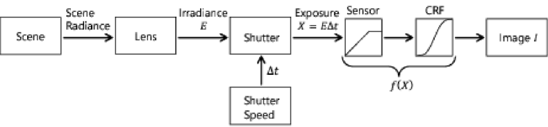
Fig. 1: Imaging pipeline of digital camera

Camera parameters, such as shutter speed and lens aperture, are usually calibrated in terms of exposure value (EV) units, and the proper exposure for a scene is automatically decided by the camera. The exposure value is commonly controlled by changing the shutter speed although it can also be controlled by adjusting various camera parameters. Here we assume that the camera parameters except for the shutter speed are fixed. Let $\nu=0\mathrm{[EV]}$ and $\Delta\tau$ be the proper exposure value and shutter speed under the given conditions, respectively. The exposure value $v_{i}\mathrm{[EV]}$ of an image taken at shutter speed $\Delta t_{i}$ is given by

$$v_{i}=\log_{2}\Delta t_{i}-\log_{2}\Delta\tau.$$ (3)

From (1) to (3), images $I_{0}$ and $I_{i}$ exposed at $0\mathrm{[EV]}$ and $v_{i}\mathrm{[EV]}$, respectively, are written as

$$I_{0}(p) =f(E(p)\Delta\tau)$$ (4)

$$I_{i}(p) =f(E(p)\Delta t_{i})=f(2^{v_{i}}E(p)\Delta\tau).$$ (5)

Assuming function $f$ is linear, we obtain the following relationship between $I_{0}$ and $I_{i}$:

$$I_{i}(p)=2^{v_{i}}I_{0}(p).$$ (6)

Therefore, the exposure can be varied artificially by multiplying $I_{0}$ by a constant. This ability is used in a new multi-exposure fusion method, which is described in the next section.

2.2 Scenario

For multi-exposure fusion methods to produce high quality images, the input images should represent the bright, middle, and dark regions of the scene. These images generally consist of a properly exposed image ($v_{i}=0\mathrm{[EV]}$), overexposed images ($v_{i}>0$), and underexposed images ($v_{i}<0$). For example, three multi-exposure images might be taken at $v_{i}=-1,0,+1\mathrm{[EV]}$. However, there are several problems in photographing multi-exposure images as follows:

• Determining appropriate exposure values for multi-exposure image fusion.

• Setting appropriate exposure values under the time of photographing when there are time constraints.

• Using an image taken at $0\mathrm{[EV]}$ that might not represent the scene properly.

The literature [22] pointed out that it is possible to improve the quality of multi-exposure images by adjusting the luminance of the images. Figure 2 shows examples of adjusted multi-exposure ones. The quality of multi-exposure images can be evaluated by using the well-exposedness [5], which indicates how well a pixel is exposed. Figure 3 shows the maximum score of the well-exposedness for each pixel in multi-exposure images. These results in Figs. 2 and 3 denote that the quality of multi-exposure images depends on the degree of adjustment. However, how to determine the degree has never been discussed.

Because of such a situation, this paper proposes a new luminance adjustment method based on automatic exposure compensation for multi-exposure fusion. In addition, we look at appropriate multi-exposure fusion methods for the adjusted multi-exposure images.

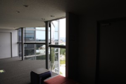
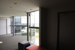
(a) Input images $I_{f}$ “Window” ($v_{i}=-1,0,+1\mathrm{[EV]}$)

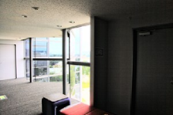
(b) Adjusted example images 1

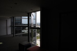
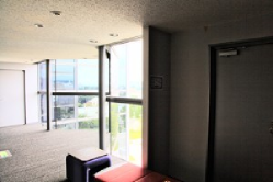
(c) Adjusted example images 2

Fig. 2: Examples of adjusted multi-exposure images

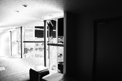
(a) Input

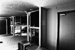
(b) Fig. 2(b)

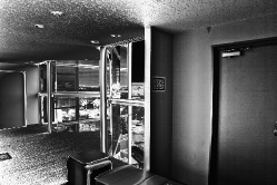
(c) Fig. 2(c)

Fig. 3: Well-exposedness map for input and enhanced multi-exposure images. A brighter pixel indicates that the pixel is well exposed.

3 Proposed luminance adjustment method

The use of the proposed method in multi-exposure fusion is illustrated in Fig. 4. To enhance the quality of multi-exposure images, local contrast enhancement is applied to luminance $L_{i}(1\leq i\leq N,i\in\mathbb{N})$ calculated from the $i$-th input image $I_{i}$, and then automatic exposure compensation and tone mapping are applied. Next, image $I_{f}$ with improved quality is produced by multi-exposure image fusion methods such as a weighted average. Here we consider input image $I_{i}$ with exposure value $v_{i}$ that satisfies $v_{i}<v_{i+1}$.

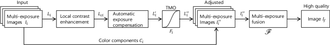
Fig. 4: Use of proposed luminance adjustment method in multi-exposure image fusion

3.1 Local contrast enhancement

If the input images do not represent the scene clearly, the quality of an image fused from them will be lower than that of an image fused from ideally exposed images. Therefore, the dodging and burning algorithm is used to enhance the local contrast[24]. The luminance $L_{ci}$ enhanced by the algorithm is given by

$$L_{ci}(p)=\frac{L_{i}^{2}(p)}{L_{ai}(p)},$$ (7)

where $L_{ai}(p)$ is the local average of luminance $L_{i}(p)$ around pixel $p$. It is obtained by applying a low-pass filter to $L_{i}(p)$. Here, a bilateral filter is used for this purpose.

$L_{ai}(p)$ is calculated using the bilateral filter:

$$L_{ai}(p)=\frac{1}{c_{i}(p)}\sum_{q\in\Omega}L_{i}(q)g_{\sigma_{1}}(q-p)g_{\sigma_{2}}(L_{i}(q)-L_{i}(p)),$$ (8)

where $\Omega$ is the set of all pixels, and $c_{i}(p)$ is a normalization term such as

$$c_{i}(p)=\sum_{q\in\Omega}g_{\sigma_{1}}(q-p)g_{\sigma_{2}}(L_{i}(q)-L_{i}(p)),$$ (9)

where $g_{\sigma}$ is a Gaussian function given by

$$g_{\sigma}(p|p=(x,y))=C_{\sigma}\exp\left(-\frac{x^{2}+y^{2}}{\sigma^{2}}\right)$$ (10)

using a normalization factor $C_{\sigma}$. Parameters $\sigma_{1}=16$ and $\sigma_{2}=3/255$ are set in accordance with [24].

3.2 Automatic exposure compensation

The purpose of the proposed exposure compensation is to automatically adjust the luminance of each input image $I_{i}$, so that adjusted images have appropriate exposure values for multi-exposure image fusion. The luminance $L^{\prime}_{i}$ of adjusted image $I^{\prime}_{i}$ is simply obtained by, according to eq. (6),

$$L^{\prime}_{i}(p)=\alpha_{i}L_{ci}(p),$$ (11)

where parameter $\alpha_{i}>0$ indicates the degree of adjustment. Next, the way to estimate the parameter $\alpha_{i}$ is described.

In $N$ input images, the $j=\lceil\frac{N+1}{2}\rceil$-th image $I_{j}$ has middle brightness, and the overexposed (or underexposed) areas in $I_{j}$ are smaller than those in the other images. Therefore, the quality of image $I_{j}$ should be better than that of the other images. We thus estimate parameter $\alpha_{j}$ from the $j$-th image in order to map the geometric mean $\overline{L}_{cj}$ of luminance $L_{cj}$ to middle-gray of the displayed image, or 0.18 on a scale from zero to one, as in [13], where the geometric mean of the luminance values indicates the approximate brightness of the image.

Let $P$ and $L(p)$ are a subset of $\Omega$ and the luminance of $p\in P$, respectively. Then the geometric mean $G(L|P)$ of luminance $L(p)$ is calculated using

$$G(L|P)=\exp{\left(\frac{1}{|P|}\sum_{p\in P}\log{\left(\max{\left(L(p),\epsilon\right)}\right)}\right)},$$ (12)

where $\epsilon$ is set to a small value to avoid singularities at $L(p)=0$. Parameter $\alpha_{j}$ is derived using eq. (12) from

$$\alpha_{j}=\frac{0.18}{G(L_{cj}|\Omega)}.$$ (13)

The adjusted version $I^{\prime}_{k}$ of the $k$-th input image $I_{k}(k\neq j)$ should describes some areas that $I^{\prime}_{j}$ could not represent well. Such areas are overexposed and underexposed regions in $I_{j}$. For this reason, we divide the luminance range of $I_{j}$ into $N$ equal parts $P_{1},\cdots,P_{N}$ as

$$P_{k}=\{p|\theta_{k}\leq L_{cj}(p)\leq\theta_{k+1}\},$$ (14)

where $\theta_{k}$ is calculated as

$$\theta_{k}=\frac{N-k+1}{N}\left(\max L_{cj}(p)-\min L_{cj}(p)\right)+\min L_{cj}(p).$$ (15)

Note that $P_{k}$ satisfies $\Omega=P_{1}\cup P_{2}\cup\cdots\cup P_{N}$. Then we adjust $I_{k}$ so that it could represent the $k$-th brightest part $P_{k}$ well. By using eqs. (12) and (14), parameter $\alpha_{k}$ is calculated as

$$\alpha_{k}=\frac{0.18}{G(L_{ck}|P_{k})}.$$ (16)

Eq. (16) enables us to produce multi-exposure images that represent not only dark areas but also bright areas.

3.3 Tone mapping

Since the adjusted luminance value $L^{\prime}_{i}(p)$ often exceeds the maximum value of the common image format, pixel values might be lost due to truncation of the values. This problem is overcome by using a tone mapping operation to fit the adjusted luminance value into the interval $[0,1]$.

The luminance $L^{\prime\prime}_{i}$ of an enhanced multi-exposure image is obtained by applying a tone mapping operator $F_{i}$ to $L^{\prime}_{i}$:

$$L^{\prime\prime}_{i}(p)=F_{i}(L^{\prime}_{i}(p)).$$ (17)

Reinhard’s global operator is used here as a tone mapping operator $F_{i}$ [13].

Reinhard’s global operator is given by

$$F_{i}(L(p))=\frac{L(p)}{1+L(p)}\left(1+\frac{L(p)}{L^{2}_{white_{i}}}\right),$$ (18)

where parameter $L_{white_{i}}>0$ determines luminance value $L(p)$ as $F_{i}(L(p))=1$. Note that Reinhard’s global operator $F_{i}$ is a monotonically increasing function. Here, let $L_{white_{i}}=\max L^{\prime}_{i}(p)$. We obtain $L^{\prime\prime}_{i}(p)\leq 1$ for all $p$. Therefore, truncation of the luminance values can be prevented.

Combining $L^{\prime\prime}_{i}$, luminance $L_{i}$ of the $i$-th input image $I_{i}$, and RGB pixel values $C_{i}(p)\in\{R_{i}(p),G_{i}(p),B_{i}(p)\}$ of $I_{i}$, we obtain RGB pixel values $C^{\prime\prime}_{i}(p)\in\{R^{\prime\prime}_{i}(p),G^{\prime\prime}_{i}(p),B^{\prime\prime}_{i}(p)\}$ of the enhanced multi-exposure images $I^{\prime\prime}_{i}$:

$$C^{\prime\prime}_{i}(p)=\frac{L^{\prime\prime}_{i}(p)}{L_{i}(p)}C_{i}(p).$$ (19)

3.4 Fusion of enhanced multi-exposure images

Enhanced multi-exposure images $I^{\prime\prime}_{i}$ can be used as input for any existing multi-exposure image fusion methods. A final image $I_{f}$ is produced as

$$I_{f}(p)=\mathscr{F}(I^{\prime\prime}_{1}(p),I^{\prime\prime}_{2}(p),\cdots,I^{\prime\prime}_{N}(p)),$$ (20)

where $\mathscr{F}(I_{1}(p),I_{2}(p),\cdots,I_{N}(p))$ indicates a function to fuse $N$ images $I_{1},I_{2},\cdots,I_{N}$ into a single image.

While numerous methods $\mathscr{F}$ for fusing images have been proposed, methods based on a weighted average are widely used [5, 10] and the weighted average is calculated as

$$\mathscr{F}(I_{1}(p),I_{2}(p),\cdots,I_{N}(p))=\frac{\sum_{i=1}^{N}w_{i}(p)I_{i}(p)}{\sum_{i=1}^{N}w_{i}(p)}.$$ (21)

Eq. (21) aims to produce high quality images by adjusting weights $w_{i}(p)$ under the condition that pixel values $I_{i}(p)$ are fixed. For example, the weight $w_{i}(p)$ is calculated on the basis of contrast, color saturation, and well-exposedness of each pixel, as in [5]. On the other hand, in the proposed method, pixel values $I_{i}(p)$ are adjusted by considering well-exposedness before the fusion. Therefore, the proposed method enables us to use simpler weights, like $w_{i}(p)=1$ referred to as “simple average”, although conventional weights are also available. In the next section, it will be shown that the simple average provides better results than conventional weights for the proposed luminance adjustment method.

4 Simulation

We evaluated the effectiveness of the proposed luminance adjustment method in terms of the quality of generated images $I_{f}$ and adjusted multi-exposure images $I^{\prime\prime}_{i}$.

4.1 Comparison with conventional methods

To evaluate the quality of the images produced by each method, objective quality assessments are needed. Typical quality assessments such as the peak signal to noise ratio (PSNR) and the structural similarity index (SSIM) are not suitable for this purpose because they use the target image with the highest quality as the reference one. We therefore used the tone mapped image quality index (TMQI) [25] and discrete entropy as quality assessments. In addition, we utilized the well-exposedness to measure the quality of adjusted multi-exposure images, as in 2.2.

TMQI represents the quality of an image tone mapped from an HDR image; the index incorporates structural fidelity and statistical naturalness. An HDR image is used as a reference to calculate structural fidelity. A reference is not needed to calculate statistical naturalness. Since the processes of tone mapping and photographing are similar, TMQI is also useful for evaluating photographs. Discrete entropy represents the amount of information in an image.

4.2 Simulation conditions

In the simulation, four photographs taken by Canon EOS 5D Mark II camera and eight photographs selected from an available online database [26] were used as input images $I_{i}$ (see Fig. 2LABEL:sub@fig:window_input). The following procedure was carried out to evaluate the effectiveness.

1. Produce $I^{\prime\prime}_{i}$ from $I_{i}$ using the proposed method.

2. Obtain $I_{f}$ fused from $I^{\prime\prime}_{i}$ by $\mathscr{F}$.

3. Compute the well-exposedness of $I^{\prime\prime}_{i}$.

4. Compute TMQI values between $I_{f}$ and $I_{H}$.

5. Compute discrete entropy of $I_{f}$.

Here we used four fusion methods, i.e., Mertens’ method [5], Sakai’s method [9], Nejati’s method [10], and the simple average, as $\mathscr{F}$.

In addition, structural fidelity in the TMQI could not be calculated due to the non-use of HDR images. Thus, we used only statistical naturalness in the TMQI for the evaluation.

4.3 Simulation results

Table 1 summarizes average scores for 12 input images in terms of statistical naturalness and discrete entropy, and the second column, “Input image”, shows average scores calculated by using input images having $0\mathrm{[EV]}$. For each score (statistical naturalness $\in[0,1]$ and discrete entropy $\in[0,8]$), a larger value means higher quality. The results indicate that the proposed method improves the quality of the fused images. It is also confirmed by comparing Fig. 5(a) with Fig. 5(b). Figure 5 also shows that the proposed method can keep the details in bright areas, and can enhance the details in dark areas.

From Table 1, it is confirmed that the simple average ($w_{i}(p)=1$) under the use of the proposed adjustment method provided the highest score of each metric in all methods, but that without the adjustment brought the worst score. Figure 6 denotes that images fused by the simple average with the proposed method represent bright areas with better quality than ones fused by the conventional methods. Hence, the proposed method can produce high quality images even when simple weights are used in eq. (21).

For these reasons, it is confirmed that the luminance adjustment is effective for multi-exposure image fusion. In addition, the use of the proposed luminance adjustment method is useful to produce high quality images which represent both bright and dark areas. Moreover, the proposed method enables us to utilize simple weights for multi-exposure image fusion, while keeping the quality of fused images.

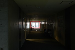
(a)

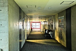
(b)

(a)

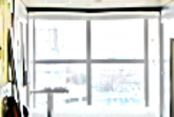
(b)

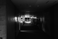
(a) Without adjustment

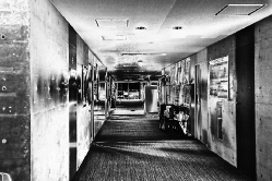
(b) Adjusted by ours

Fig. 5: Comparison among luminance adjustment methods under the use of Nejati’s fusion method [10]. Top to bottom: fused image $I_{f}$, zoom-in view of $I_{f}$, and well-exposedness map for adjusted multi-exposure images $I^{\prime\prime}_{i}$. For well-exposedness map, a brighter pixel indicates that the pixel is well exposed.

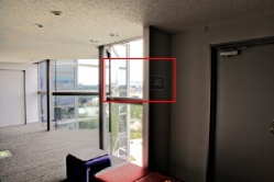
(a)

(b)

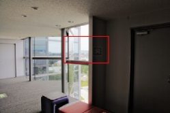
(c)

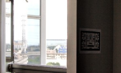
(a)

(b)

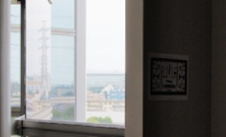
(c)

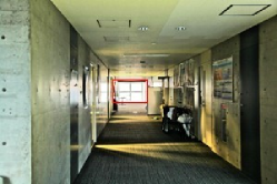
(a)

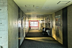
(b)

(c)

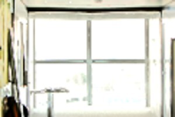
(a) Mertens [5]

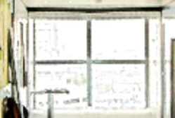
(b) Sakai [9]

(c) Simple average

Fig. 6: Comparison among multi-exposure fusion methods under the use of the proposed method

Table 1: Experimental results. Boldface indicates the higher score. “Without” means that images $I_{f}$ are produced without luminance adjustment

Method	Input	Mertens [5]		Sakai [9]		Nejati [10]		Simple average
3-10	image	Without	Ours	Without	Ours	Without	Ours	Without	Ours
Statistical	0.092	0.083	0.179	0.079	0.173	0.089	0.179	0.045	0.278
Naturalness
Discrete	5.199	6.259	6.952	6.270	6.968	6.232	6.920	5.601	7.071
entropy

5 Conclusion

This paper has proposed a novel luminance adjustment method based on automatic exposure compensation for multi-exposure fusion. The proposed method automatically adjusts the luminance of input multi-exposure images to suitable ones for multi-exposure fusion. The proposed method also enables us to utilize simple weights for multi-exposure image fusion, while keeping the quality of fused images. Experimental results have showed the effectiveness of the luminance adjustment for multi-exposure image fusion in terms of the well-exposedness. Moreover, it has been confirmed that fusion methods can produce high quality images under the use of the proposed luminance adjustment method, in terms of statistical naturalness and discrete entropy.

References

- [1] K. Zuiderveld, “Contrast limited adaptive histograph equalization,” in Graphics gems IV. Academic Press Professional, Inc., 1994, pp. 474–485.
- [2] X. Wu, X. Liu, K. Hiramatsu, and K. Kashino, “Contrast-accumulated histogram equalization for image enhnacement,” in 2017 International Conference on Image Processing (ICIP). IEEE, 2017, pp. 3190–3194.
- [3] Y. Kinoshita, T. Yoshida, S. Shiota, and H. Kiya, “Pseudo multi-exposure fusion using a single image,” in APSIPA Annual Summit and Conference, 2017, pp. 263–269.
- [4] A. A. Goshtasby, “Fusion of multi-exposure images,” Image and Vision Computing, vol. 23, no. 6, pp. 611–618, 2005.
- [5] T. Mertens, J. Kautz, and F. Van Reeth, “Exposure fusion: A simple and practical alternative to high dynamic range photography,” Computer Graphics Forum, vol. 28, no. 1, pp. 161–171, 2009.
- [6] A. Saleem, A. Beghdadi, and B. Boashash, “Image fusion-based contrast enhancement,” EURASIP Journal on Image and Video Processing, vol. 2012, no. 1, p. 10, 2012.
- [7] J. Wang, G. Xu, and H. Lou, “Exposure fusion based on sparse coding in pyramid transform domain,” in Proceedings of the 7th International Conference on Internet Multimedia Computing and Service, ser. ICIMCS ’15. New York, NY, USA: ACM, 2015, pp. 4:1–4:4.
- [8] Z. Li, J. Zheng, Z. Zhu, and S. Wu, “Selectively detail-enhanced fusion of differently exposed images with moving objects,” IEEE Transactions on Image Processing, vol. 23, no. 10, pp. 4372–4382, 2014.
- [9] T. Sakai, D. Kimura, T. Yoshida, and M. Iwahashi, “Hybrid method for multi-exposure image fusion based on weighted mean and sparse representation,” in 2015 23rd European Signal Processing Conference (EUSIPCO). EURASIP, 2015, pp. 809–813.
- [10] M. Nejati, M. Karimi, S. M. R. Soroushmehr, N. Karimi, S. Samavi, and K. Najarian, “Fast exposure fusion using exposedness function,” in 2017 International Conference on Image Processing (ICIP). IEEE, 2017, pp. 2234–2238.
- [11] K. Ram Prabhakar, V. Sai Srikar, and R. Babu, “Deepfuse: A deep unsupervised approach for exposure fusion with extreme exposure image pairs,” in 2017 International Conference on Computer Vision (ICCV). IEEE, 2017, pp. 4724–4732.
- [12] P. E. Debevec and J. Malik, “Recovering high dynamic range radiance maps from photographs,” in ACM SIGGRAPH. ACM, 1997, pp. 369–378.
- [13] E. Reinhard, M. Stark, P. Shirley, and J. Ferwerda, “Photographic tone reproduction for digital images,” ACM Transactions on Graphics (TOG), vol. 21, no. 3, pp. 267–276, 2002.
- [14] T.-H. Oh, J.-Y. Lee, Y.-W. Tai, and I. S. Kweon, “Robust high dynamic range imaging by rank minimization,” IEEE Transactions on Pattern Analysis and Machine Intelligence, vol. 37, no. 6, pp. 1219–1232, 2015.
- [15] Y. Kinoshita, S. Shiota, M. Iwahashi, and H. Kiya, “An remapping operation without tone mapping parameters for hdr images,” IEICE Transactions on Fundamentals of Electronics, Communications and Computer Sciences, vol. 99, no. 11, pp. 1955–1961, 2016.
- [16] Y. Kinoshita, S. Shiota, and H. Kiya, “Fast inverse tone mapping with reinhard’s grobal operator,” in 2017 IEEE International Conference on Acoustics, Speech and Signal Processing (ICASSP). IEEE, 2017, pp. 1972–1976.
- [17] ——, “Fast inverse tone mapping based on reinhard’s global operator with estimated parameters,” IEICE Transactions on Fundamentals of Electronics, Communications and Computer Sciences, vol. 100, no. 11, pp. 2248–2255, 2017.
- [18] Y. Q. Huo and X. D. Zhang, “Single image-based hdr imaging with crf estimation,” in 2016 International Conference On Communication Problem-Solving (ICCP). IEEE, 2016, pp. 1–3.
- [19] T. Murofushi, M. Iwahashi, and H. Kiya, “An integer tone mapping operation for hdr images expressed in floating point data,” in 2013 IEEE International Conference on Acoustics, Speech and Signal Processing (ICASSP). IEEE, 2013, pp. 2479–2483.
- [20] T. Murofushi, T. Dobashi, M. Iwahashi, and H. Kiya, “An integer tone mapping operation for hdr images in openexr with denormalized numbers,” in 2014 IEEE International Conference on Image Processing (ICIP). IEEE, 2014, pp. 4497–4501.
- [21] T. Dobashi, T. Murofushi, M. Iwahashi, and K. Hitoshi, “A fixed-point global tone mapping operation for hdr images in the rgbe format,” IEICE Transactions on Fundamentals of Electronics, Communications and Computer Sciences, vol. 97, no. 11, pp. 2147–2153, 2014.
- [22] Y. Kinoshita, T. Yoshida, S. Shiota, and H. Kiya, “Multi-exposure image fusion based on exposure compensation,” in 2018 IEEE International Conference on Acoustics, Speech and Signal Processing (ICASSP). IEEE, 2018, pp. 1388–1392.
- [23] F. Dufaux, P. L. Callet, R. Mantiuk, and M. Mrak, High Dynamic Range Video, From Acquisition, to Display and Applications. Elsevier Ltd., 2016.
- [24] H. Youngquing, Y. Fan, and V. Brost, “Dodging and burning inspired inverse tone mapping algorithm,” Journal of Computational Information Systems, vol. 9, no. 9, pp. 3461–3468, 2013.
- [25] H. Yeganeh and Z. Wang, “Objective quality assessment of tone mapped images,” IEEE Transactions on Image Processing, vol. 22, no. 2, pp. 657–667, 2013.
- [26] “easyhdr.” [Online]. Available: https://www.easyhdr.com/