Topological Laminations on Surfaces

Abstract

We present and prove a topological characterization of geodesic laminations on hyperbolic surfaces of finite type.

1 Introduction

Geodesic laminations on hyperbolic surfaces were defined by Thurston in the early seventies [1, Sect. 8.5], and have proved since to be an important tool in low-dimensional topology [1, 2, 3, 4]:

Definition 1.

A geodesic lamination $\cal L$ on a hyperbolic surface $\Sigma$ is a non-empty closed subset of $\Sigma$ which is a union of simple and pairwise disjoint complete geodesics.

This definition is short and simple. However, the geodesics in a lamination, seen as curves, have the following important homotopical property: they can be continuously deformed onto embedded finite graphs, satisfying specific differentiability conditions and called train tracks, that is, geodesic laminations are carried by train-tracks [1, 5]. This property led Hatcher to redefine a measured lamination as a curve set carried by a train track taken among finitely many predefined ones, in order to directly obtain results independent of the choice of a metric [6]. Other metric independent results have been proved more recently [7], again using this property. Behind these results is the fact that geodesic laminations can be topologically characterized, a characterization that we make explicit as follows:

Definition 2.

A topological lamination $\cal T$ on a surface $\Sigma$ is a non-empty subset of $\Sigma$ which is a union of simple and pairwise disjoint curves, all closed or two-way infinite, such that the curves are pairwise non-homotopic, they are all carried by a common train track $\Gamma$, and $\cal T$ is maximal for this $\Gamma$ and remains so after any isotopies applied to the curves.

The above definition is about ordinary continuous curves, and the train track condition is combinatorial, as train tracks can be seen as plain embedded graphs together with vertex crossing rules for the carried paths. Moreover, quite remarkably, the topological hypothesis of being closed in Definition 1 becomes the setwise hypothesis of being maximal with respect to set inclusion in Definition 2.

Now, although it is admitted that geodesic laminations can be characterized up to isotopy as in Definition 2 (see [1, Prop. 8.9.4] for a result in this direction), to the knowledge of the author this fact has not been proved, not even explicitly written down. Such a characterization shows nevertheless some advantages. Not only maximality gives an alternative way of checking that a set of curves is a lamination, but also a combinatorial viewpoint of laminations is made visible and can be exploited for itself. In particular, by labeling the edges of the train tracks, laminations can be made into usual shifts, creating bridges towards symbolic dynamics and word combinatorics [8, 9, 10, 11].

The aim of this paper is to present a detailed exposition of the proof of the equivalence up to isotopy between Definitions 1 and 2. Noteworthily, in the course of this proof two issues specific to topological laminations are raised: Defining a notion of complementary region, and dealing with non-compact leaves homotopic to compact curves. We also prove that a topological lamination carried by a train track $\Gamma$ can be moved by an ambient isotopy into a regular neighborhood of $\Gamma$ (see Proposition 5.10). This latter result says that laminations can be described with respect to fat graphs (equiv. ribbon graphs) [12, 13], relaxing their dependency to the surfaces themselves, and thus making laminations even more combinatorial objects.

2 Basic Definitions

2.1 Surfaces and PL structures

A surface of finite type is a closed surface from which finitely many points, the punctures, have been removed. All the surfaces of finite type except the torus and the sphere admit complete metrics with constant curvature $-1$, making them hyperbolic surfaces, but only those whose area is finite are called hyperbolic surfaces of finite type. Hyperbolic surfaces all share the same universal covering space, the hyperbolic plane $\mathbb{H}^{2}$, so they are quotients of $\mathbb{H}^{2}$ by discrete subgroups of isometries acting properly and discontinuously, without fixed points in $\mathbb{H}^{2}$. A subsurface, closed as a subset of a complete hyperbolic surface and whose frontier components are geodesics, is called a hyperbolic surface with geodesic boundary, and so is any surface isometric (in the Riemannian sense) to it.

A topological manifold is triangulable if it is homeomorphic to a simplicial complex. When in addition the simplicial complex admits an atlas such that one can pass from chart to chart by piecewise linear functions, the manifold together with the complex is called a PL manifold, and one says the triangulation is PL. A piecewise linear map between PL manifolds is called a PL map. It is known that every manifold of dimension no more than 3 is triangulable and that every triangulation is PL in a unique way up to PL homeomorphism. Thus a tessellation of a hyperbolic surface of finite type $\Sigma$ by hyperbolic triangles defines a PL structure, which is unique, though there are many non-equivalent hyperbolic structures on $\Sigma$. Likewise, the universal covering by $\mathbb{H}^{2}$ of $\Sigma$, gives it a differentiable, or smooth structure which is unique up to diffeomorphism. In the sequel $\Sigma$ is assumed to be endowed with both its PL and smooth structures.

2.2 Curves, Geodesics and Laminations

A (PL) curve $\gamma$ on a surface $\Sigma$ is a (PL) continuous map, either from a closed connected subset $J$ of the real line, or from the circle to $\Sigma$. In the latter case $\gamma$ is said to be closed; if the map defining the curve is injective, $\gamma$ is said to be simple; if $\gamma$ is simple, closed, and bounds neither a disk nor a once punctured disk it is said to be essential; if $J=\mathbb{R}$, $\gamma$ is said to be two-way infinite; if $J=\mathbb{R}_{\geq 0}$ or $J=\mathbb{R}_{\leq 0}$ , $\gamma$ is said to be one-way infinite; if $J$ is bounded and $\gamma$ is simple then $\gamma$ is called an arc.

The geometric model we use for $\mathbb{H}^{2}$ is the Poincaré disk model: Topologically it is the interior of the compact unit disk $D^{2}$ in the Euclidean plane, the boundary circle $\partial D^{2}$ is then called the circle at infinity. The complete geodesics in $\mathbb{H}^{2}$ are the open diameters, and the open arcs of circle orthogonal to $\partial D^{2}$. The two frontier points of a geodesic lie on the circle at infinity and are called its endpoints. The complete geodesics in a hyperbolic surface of finite type $\Sigma$ are the projections of the complete geodesics in $\mathbb{H}^{2}$ by the universal covering map. A complete geodesic in $\mathbb{H}^{2}$ becomes a curve as soon as a base point, and a tangent vector at it (i.e. a direction on the geodesic) have been chosen, the parametrization by $\mathbb{R}$ being given by the directed distance from the base point on the geodesic. A complete geodesic in $\Sigma$ inherits a parametrization from any of its lifts to $\mathbb{H}^{2}$. If the geodesic is compact, any such parametrization is a periodic map, hence it can be made into a map from $S^{1}$ to $\Sigma$, that is, the geodesic can be made into a closed curve, and it is then called a closed geodesic. A curve, or arc contained in a complete geodesic and parametrized by length is called a geodesic curve, or a geodesic arc.

When they belong to a geodesic lamination $\cal L$, the geodesics are called the leaves of $\cal L$. Likewise, the curves in a topological lamination are called its leaves. The complement of $\cal L$ is a union of connected components, called the complementary regions (or principal regions in [2]) of $\cal L$ in $\Sigma$, and it has same area as $\Sigma$, i.e. $\cal L$ has zero area [14]. A complementary region $U$ is the interior of a hyperbolic surface with geodesic boundary [14, Lem. 4.2.6].

A leaf of $\cal L$ isolated from the rest of $\cal L$ at least from one side is called a boundary leaf, and a boundary leaf isolated from the rest of $\cal L$ from both sides is called an isolated leaf. The connected components of the frontier in $\Sigma$ of the complementary regions all correspond (not necessarily bijectively) to the boundary leaves [14, Lem. 4.2.6]. A connected component of the frontier of a complementary region contains at least one boundary leaf, but it may also contain non-boundary leaves at which boundary leaves accumulate (this happens to compact leaves around which isolated leaves spiral from both sides), a leaf contained in a connected component of the frontier of a complementary region is called a frontier leaf. The number of complementary regions of $\cal L$ is finite, as is the number of boundary leaves [14, Cor. 4.2.7]. The set of geodesics obtained by removing from $\cal L$ the (finitely many) isolated leaves is still a geodesic lamination ${\cal L}^{\prime}$, called the derived lamination of $\cal L$ in [2]. The derived lamination is always a lamination with compact support, which means that no leaf of ${\cal L}^{\prime}$ ends up at a puncture (thus in particular there are only finitely many leaves of $\cal L$ ending up at a puncture), moreover ${\cal L}^{\prime\prime\prime}={\cal L}^{\prime\prime}$ (so that the number of frontier leaves of $\cal L$ is finite too), finally, if $\cal L$ has no compact leaf then ${\cal L}^{\prime\prime}={\cal L}^{\prime}$ [14, Th. 4.2.8].

2.3 Graphs and Train Tracks

A graph is defined by a set of vertices, a set of edges, and a map mapping each edge to an unordered pair of (not necessarily distinct) vertices; when the pair of vertices of an edge is ordered, the edge is said to be directed, the smaller vertex is then called its origin and the bigger one its end. An embedding of a graph in a surface $\Sigma$ is a pair of maps, one sending the vertices into $\Sigma$ union its punctures, and the other one sending the edges to simple curves in $\Sigma$, in such a way that the endpoints of each curve are the images of the vertices of its corresponding edge, and the curves may meet only at their endpoints. When a graph is embedded, we identify it with its image by the embedding. A train track [1, 5] is a finite embedded graph such that: The edges are $C^{1}$ curves, there is a well-defined tangent space at every vertex in $\Sigma$ (see Figure 1), and no connected component of $\Gamma$’s complement in $\Sigma$ is one of the following forbidden regions:

• a disk whose frontier, as a curve has less than three points where it is not $C^{1}$ (punctures count as such points)

• an annulus whose two frontier components, as curves are closed $C^{1}$

• a once punctured disk whose frontier component, as a curve is closed $C^{1}$

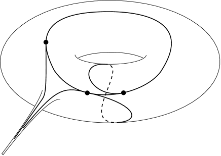
Figure 1: A train track on a once punctured torus with four vertices (one is the puncture) and six edges

We also make use of infinite train tracks in $\mathbb{H}^{2}$, but they are always preimages by the universal covering map of ordinary, that is, finite train tracks on a hyperbolic surface of finite type.

A path on a graph is a set of directed edges indexed by a subset of consecutive integers in $\mathbb{Z}$, in such a way that for every pair of edges indexed by a pair $(i,i+1)$, the end of the edge $i$ is the origin of the edge $i+1$. A path on an embedded graph is also a curve as soon as a base point is chosen, the parametrization coming from the edge embeddings. On a train track, an admissible edge path, or a trainpath for some authors [5], is a path everywhere $C^{1}$ as a curve, such that no two consecutive edges share a puncture (i.e. admissible paths ‘do not cross’ punctures). From now on, by a path on a train track we always mean an admissible edge path. A connected train track is a train track of whose any two vertices can be joined by a path.

2.4 Homotopy

An ambient isotopy of a topological space is a homotopy $H$ between the identity map and a self-homeomorphism $\varphi$ of the space such that for each $t\in[0,1]$, $H(\cdot,t)$ is a self-homeomorphism. Given a subset $B$ of the space, $B$ and $\varphi(B)$ are then said ambient isotopic. On surfaces train tracks and laminations are considered up to ambient isotopy. Note that if two embeddings of the same finite graph in a hyperbolic surface of finite type $\Sigma$ are isotopic, it is possible to make an ambient isotopy involving only a neighborhood of $\Sigma$’s punctures in such a way that both coincide in this neighborhood. Then, since the complement of such a neighborhood is a compact surface, there is an ambient isotopy deforming one embedding onto the other one [15, §4, Cor.3 and 4]. Hence, when we deform a train track onto another one by some isotopy, we will just check that the edges are $C^{1}$ in both train tracks, and that the tangent spaces are well-defined and are compatible at the corresponding vertices.

In this paper, two arbitrary curves are said homotopic (resp. isotopic) if they admit parametrizations making them homotopic (resp. isotopic) using a uniformly continuous map. This additional condition is made necessary by the definitions of carrying, that we give and comment on in the next subsection, and by the fact that the curves we consider may not be compact. As said before, choosing a base point on a path on a train track, resp. a base point and a direction on a geodesic, yields a parametrization as a curve for the path, resp. the geodesic. Now, a change of base point can be realized by a homotopy, in the above sense, between the two parametrized curves, so we can speak about homotopy between a curve and a path considered up to index translation, and similarly between a curve and a geodesic. As for geodesics, note that a curve homotopic to a complete geodesic in a surface is necessarily either two-way infinite or closed.

Homotopies between curves and paths on a train track $\Gamma$ lift to $\mathbb{H}^{2}$, as homotopies between curves and paths on the preimage $\tilde{\Gamma}$ of $\Gamma$ by the universal covering map. (See Figure 2)

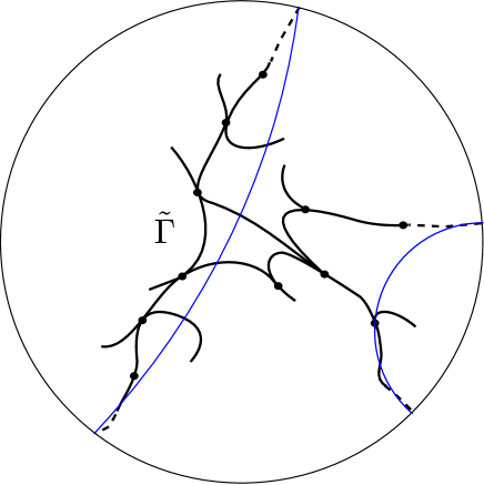
Figure 2: Part of the preimage $\tilde{\Gamma}$ in $\mathbb{H}^{2}$ (in bold lines) of a train track $\Gamma\subset\Sigma$, with two complete geodesics (in thin lines) homotopic to paths on $\tilde{\Gamma}$

The following lemma is known for compact hyperbolic surfaces with geodesic boundary [7, Lem. 20], and can be derived from it.

Lemma 2.1.

On a hyperbolic surface of finite type, (1) any path on a train track $\Gamma$ lifts to an embedded path in $\tilde{\Gamma}$, (2) any two paths in $\tilde{\Gamma}$ which diverge at some vertex never meet again, and (3) every path in $\tilde{\Gamma}$ is homotopic to a (unique) geodesic.

Proof. The first two assertions are combinatorial, and will follow easily from the construction presented below, only the third one needs a topological argument.

Let $\Sigma$ be a non-compact hyperbolic surface of finite type, with a train track $\Gamma$ on it. Take a union of pairwise disjoint open neighborhoods of $\Sigma$’s punctures in such a way that this union is allowed to meet only the non-compact edges of $\Gamma$, and along at most one curve for each edge. We further ask that removing these neighborhoods results in a (necessarily compact) surface $\Sigma^{\prime}$ with $C^{\infty}$ boundary, so that the Riemannian metric of $\Sigma$ induces one on $\Sigma^{\prime}$. We change the metric on $\Sigma^{\prime}$ in order to make it into a hyperbolic surface with geodesic boundary $\Sigma^{\prime}_{h}$. Since $\Sigma^{\prime}$ is compact the two metrics are Lipschitz equivalent. Next, in $\Sigma$ we remove from $\Gamma$ the non-compact edges if any, and inductively, the vertices where the tangent space has become undefined as well as the edges adjacent to them. If the resulting graph, necessarily in $\Sigma^{\prime}_{h}$, is empty, this implies that there are only finitely many two-way infinite paths on $\Gamma$, each path being homotopic to a geodesic joining two punctures, and the conclusions of the lemma obviously hold. If the resulting graph is not empty, it is a disjoint union $\Gamma^{\prime}$ of compact train tracks in $\Sigma^{\prime}_{h}$, to each of which [7, Lem. 20] applies, hence the first two conclusions of the lemma hold for $\Gamma^{\prime}$ in $\Sigma^{\prime}$. The third one holds by Lipschitz equivalence of the metrics. Note that no component of $\partial\Sigma_{h}$ is carried by $\Gamma^{\prime}$, for if that was the case there would be a forbidden region in the complementary set of $\Gamma$, in particular any path carried by the preimage $\tilde{\Gamma^{\prime}}$ of $\Gamma^{\prime}$ by the universal covering (of $\Sigma$) has two distinct endpoints on the circle at infinity. Now we add back to $\Sigma^{\prime}$ the punctured neighborhoods and to $\Gamma^{\prime}$ the removed vertices and edges. Taking into account that these edges involve only paths ending up at punctures, and that a path joining a vertex to a puncture has finitely many edges, the lemma is proved. $\diamondsuit$

It is a consequence of the above lemma, that any two paths on a train track which are homotopic differ by an index translation in $\mathbb{Z}$. In other words, up to index translation there is only one path homotopic to a given curve.

2.5 Carrying

The definitions of carrying do not need the notion of lamination, so we state them for sets of curves. A set of everywhere smooth curves is carried by a train track $\Gamma$ if there is a $C^{1}$ map from $\Sigma$ to itself homotopic to the identity, non-singular on the tangent space of each curve, sending each curve to a path on $\Gamma$ [1, Def. 8.9.1]. There are two more notions of carrying, valid for curves not necessarily everywhere smooth.

The first one, already used by Thurston is strong carrying (we use the terminology of [7]). A set of curves $\cal C$ in a surface $\Sigma$ is strongly carried by a train track $\Gamma$ if there is a regular neighborhood $N\supset{\cal C}$ of $\Gamma$ realized as a disjoint union of piecewise $C^{1}$, or PL arcs, called fibers, to which every path on $\Gamma$ is everywhere transverse, and such that each curve of ${\cal C}$ is also everywhere transverse to the fibers [5, 7] (see Figure 3); $N$ is called a fibered neighborhood of $\Gamma$. Here, since regular neighborhoods and transversality are used, the smooth, or PL structures of $\Sigma$ are necessary, and accordingly the carried lamination has to be piecewise $C^{1}$, or PL. It is a fundamental result that every geodesic lamination (hence formed of everywhere smooth curves) on a hyperbolic surface of finite type has strongly carrying train tracks [1, Sect. 8.9], [5, Th.1.6.5]. The link between carrying and strong carrying is the following: For every lamination carried by a train track $\Gamma$ there is a homeomorphism of $\Sigma$ isotopic to the identity map which sends it onto a lamination strongly carried by $\Gamma$ [1], so these two notions of carrying are close.

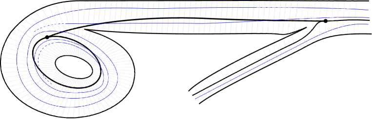
Figure 3: A fibered neighborhood of a train track near two vertices, with three pieces of strongly carried leaves

The second notion of carrying is weak carrying: a set of curves $\cal C$ on $\Sigma$ is weakly carried by a train track $\Gamma$ if each curve in $\cal C$, is homotopic to a path on $\Gamma$ [7]. Weak carrying uses homotopies which are uniformly continuous maps, so there is a priori a dependency on the uniform structure induced by $\Sigma$’s metric space structure, however it is known that a change of hyperbolic metric on a hyperbolic surface of finite type always induces a Lipschitz equivalent metric space structure. For weak carrying, as the terminology suggests we have the following:

Lemma 2.2.

Strong carrying implies weak carrying.

Proof. The way curves are deformed onto paths is not a part of the definition of strong carrying, however there are natural homotopies: The ones obtained by sliding each curve along the transverse fibers towards the train track. Now, on a hyperbolic surface of finite type there are always regular neighborhoods of the train track which can be fibered in such a way that the fibers have uniformly bounded lengths, so these natural homotopies can be taken to be uniformly continuous, and strong carrying implies weak carrying. $\diamondsuit$

And also:

Lemma 2.3.

Carrying implies weak carrying.

Proof. A map realizing the carrying by some train track of a lamination made of smooth curves can be modified in a neighborhood of the punctures so as to become uniformly continuous, so carrying also implies weak carrying. $\diamondsuit$

In Definition 2 by carrying we mean weak carrying, so according to the above lemmas, the equivalence between Definitions 1 and 2 holds for the three forms of carrying.

3 A Topological Lamination is Isotopic to a Geodesic Lamination

In this section by ‘surface’ we mean a hyperbolic surface of finite type. We begin with a lemma which allows making topological curves into PL ones. It proves useful for the subsequent results since it allows the use of general position arguments from PL Topology:

Lemma 3.1.

For any simple infinite curve in a surface $\Sigma$, there is an isotopy making it a PL curve. If the curve is a one-way infinite curve ending up at a puncture in a leaf of a topological lamination, the isotopy can be realized by an ambient isotopy avoiding the rest of the lamination.

The proof uses methods of classical planar topology, but it is quite long and technical, so we postpone it to the Appendix. This lemma has the following corollary:

Corollary 3.2.

Let $\gamma$ be a two-way infinite (resp. closed) curve in a surface $\Sigma$ homotopic to a two-way infinite (resp. closed) geodesic, then $\gamma$ is isotopic to it.

Proof. For closed curves, according to [16, Th. A1] we can suppose $\gamma$ is PL, and since a closed curve homotopic to a closed geodesic is essential, [16, Th. 2.1] gives the desired isotopy. Now let $\gamma$ be two-way infinite, and $\gamma_{g}$ be the geodesic homotopic to it. Let $\gamma^{\prime}$ be a PL curve isotopic to $\gamma$ given by Lemma 3.1, then it suffices to prove that $\gamma^{\prime}$ is isotopic to $\gamma_{g}$. We lift these two curves to $\mathbb{H}^{2}$ in such a way that the two lifts $\tilde{\gamma^{\prime}}$ and $\tilde{\gamma_{g}}$ share the same two endpoints on the circle at infinity. As a first case, if $\gamma^{\prime}$ and $\gamma_{g}$ are disjoint, then $\tilde{\gamma^{\prime}}$ and $\tilde{\gamma_{g}}$ bound an infinite stripe $\mathbb{R}\times[0,1]$, which embeds in $\Sigma$ by the covering projection since the image of $\mathbb{R}\times\{0,1\}$, which is $\gamma^{\prime}\cup\gamma_{g}$ does, and this provides the desired isotopy. The second case is when $\gamma^{\prime}$ and $\gamma_{g}$ intersect; then we put them in general position, and the intersections of $\tilde{\gamma^{\prime}}$ with the translates of $\tilde{\gamma_{g}}$ delimit in $\mathbb{H}^{2}$ an enumerable number of disks, any two of which are either nested or have disjoint interiors. Then the innermost ones all embed in $\Sigma$ by the covering projection, so they can be used to perform inductively isotopies in $\Sigma$ until all intersections are erased, making $\gamma^{\prime}$ and $\gamma_{g}$ disjoint curves, and by the first case above there is an isotopy between these two curves.$\diamondsuit$

This corollary suggests that in Definition 2, the term “isotopies” could be replaced by “homotopies”. But there is a subtlety here: A closed curve is parametrized by $S^{1}$, as well as by $\mathbb{R}$, using a periodic map. Then, for instance an embedded two-way infinite curve spiraling along a closed geodesic in a compact annulus in $\Sigma$ is homotopic to this geodesic. However there can be no isotopy, since one map is an embedding of $\mathbb{R}$ and the other one is not. This is why in the statement of the following Proposition 3.3, homotopies are used instead of isotopies. Nevertheless, up to a convention that we will make after Corollary 3.5, this proposition proves one direction of the equivalence:

Proposition 3.3.

Let $\cal T$ be a topological lamination on a surface $\Sigma$. Then $\cal T$ can be deformed onto a geodesic lamination $\cal L$ by curve-by-curve homotopies.

Proof. Let $\cal T$ be a topological lamination weakly carried by a train track $\Gamma$, as in Definition 2. We denote by $p:\mathbb{H}^{2}\rightarrow\Sigma$ the universal covering, and by $\tilde{\Gamma}$ a component of $p^{-1}(\Gamma)$. Since each of $\cal T$’s curves has a lift homotopic to one path on $\tilde{\Gamma}$, which is homotopic to a geodesic by Lemma 2.1, $\cal T$ can be deformed by curve-by-curve homotopies onto a set ${\cal L}_{0}$ of geodesics. The geodesics in this set are simple and pairwise disjoint, because their corresponding curves in $\cal T$ are, and the closure in $\Sigma$ of a set of pairwise disjoint simple geodesics is a geodesic lamination $\cal L$ [2, Lem. 3.2]. Suppose there is a geodesic $\gamma$ in ${\cal L}\setminus{\cal L}_{0}$, then $\gamma$ is the pointwise limit of a sequence $\{\gamma_{n}\}_{n\in\mathbb{N}}$ of geodesics in ${\cal L}_{0}$. We lift the $\gamma_{n}$ and $\gamma$ to geodesics $\{\tilde{\gamma}_{n}\}_{n\in\mathbb{N}}$ and $\tilde{\gamma}$ in $\mathbb{H}^{2}$ in such a way that the pairs of endpoints of the $\tilde{\gamma}_{n}$ lie among those of $\tilde{\Gamma}$’s paths and converge to the pair of endpoints of $\tilde{\gamma}$, and since each $\tilde{\gamma}_{n}$ has a unique corresponding path on $\tilde{\Gamma}$ with same endpoints, $\tilde{\gamma}$ has also an associated path $\tilde{\delta}$ with same endpoints. Again by Lemma 2.1, $\tilde{\gamma}$ is homotopic to $\tilde{\delta}$, hence $\gamma$ is homotopic to the path $\delta=p(\tilde{\delta})$.

If each curve in $\cal T$, closed or two-way infinite, has its corresponding geodesic in $\cal L$ accordingly closed or two-way infinite, we apply Corollary 3.2 to deduce that ${\cal L}_{0}$ is isotopic to $\cal T$ by leaf-by-leaf isotopies. Now, $\Gamma$ carries ${\cal L}_{0}\cup\gamma$, but this contradicts the fact that $\cal T$ should remain maximal with respect to being carried by $\Gamma$, whatever the isotopies applied to its curves, hence there is no such geodesic as $\gamma$, so ${\cal L}_{0}=\cal L$.

If there are two-way infinite curves in $\cal T$ homotopic to closed geodesics (necessarily finite in number) we denote these geodesics by $\gamma_{i},i=1,\cdots,k$, and we consider $k$ pairwise disjoint closed annulus neighborhoods of the $\gamma_{i}$. We first make an isotopy in each annulus in order to move all the curves of ${\cal L}_{0}\cup\gamma$ other than the $\gamma_{i}$ away from them, without creating intersections among the curves. Next, in the annuli we replace the $\gamma_{i}$ by homotopic spiraling two-way infinite simple curves; we obtain in this way a set of curves ${\cal L}_{1}\cup\gamma^{\prime}$. Now, according to Corollary 3.2, these spiraling curves are isotopic to their corresponding curves in $\cal T$, so that ${\cal L}_{1}$ is isotopic curve by curve to $\cal T$. However, the set of pairwise disjoint pairwise non-homotopic curves ${\cal L}_{1}\cup\gamma^{\prime}$ is carried by $\Gamma$, again contradicting maximality of $\cal T$’s carrying. Hence here too ${\cal L}_{0}={\cal L}$. $\diamondsuit$

The key-fact with this proposition, is that it provides a natural bijection between the leaves of a given topological lamination $\cal T$ in $\Sigma$ and those of a unique geodesic lamination $\cal L$, and this allows defining the boundary leaves, the isolated leaves and the frontier leaves of $\cal T$ as the leaves homotopic to the boundary leaves, isolated leaves, and frontier leaves respectively, of $\cal L$. The frontier leaves of $\cal T$ lift through $p$, the universal covering map, to $\mathbb{H}^{2}$, and (using the Schoenflies Theorem) they delimit disks in $\mathbb{H}^{2}$ union the circle at infinity such that their interiors contain no lift of $\cal T$’s leaves. This leads to:

Definition 3.

Let $\cal T$ be a topological lamination on a surface $\Sigma$, and $\tilde{E}$ be an open disk in $\mathbb{H}^{2}$ bounded by lifts of $\cal T$’s frontier leaves such that $\tilde{E}$ contains no lift of a leaf of $\cal T$. The image of $\tilde{E}$ by $p$ is called a complementary region of $\cal T$.

The complementary regions are open sets, finite in number, but unlike for geodesic laminations their union need not be equal to $\Sigma\setminus\cal T$ (it may even not be a full measure set in $\Sigma$).

Lemma 3.4.

Let $\cal T$ be a topological lamination on a surface $\Sigma$. If a two-way infinite leaf $\gamma$ of $\cal T$ is homotopic to a simple closed geodesic $\gamma_{g}$, there is a complementary region $E$ of $\cal T$ such that $E\cup\gamma$ contains a compact annulus whose boundary components are PL curves homotopic to $\gamma$.

Proof. Note that a closed leaf in a geodesic lamination is always a frontier leaf, so $\gamma_{g}$ is in the geodesic lamination corresponding to $\cal T$ given by Proposition 3.3, thus $\gamma$ is a frontier leaf for $\cal T$. The fundamental group of $\Sigma$ is considered at a base point $x\in\gamma_{g}$. Topologically, the cyclic covering $\Sigma_{\gamma_{g}}$ corresponding to the homotopy class of $\gamma_{g}$ is an open annulus, whose fundamental group $G_{c}\cong\mathbb{Z}$ is generated by the homotopy class of a lift $\hat{\gamma_{g}}$ of $\gamma_{g}$ at some point $\hat{x}$ over $x$. From now on, we denote the elements of $G_{c}$ by the integers in $\mathbb{Z}$ they correspond to. Lifting the homotopy between $\gamma$ and $\gamma_{g}$ to $\Sigma_{\gamma_{g}}$ gives a curve $\hat{\gamma}$ in $\Sigma_{\gamma_{g}}$, that we lift further to $\mathbb{H}^{2}$ to obtain a family of curves $\{\tilde{\gamma_{i}}\}_{i\in G_{c}}$, all sharing the same two endpoints on the circle at infinity, and all pairwise disjoint, because $\hat{\gamma}$ is simple. Each pair of consecutive $\tilde{\gamma_{i}}$, $(\tilde{\gamma_{i}},\widetilde{\gamma_{i+1}})$ bounds an open disk $\tilde{E_{i}}$, and $\tilde{E_{i}}$ projects via the universal covering to a connected open set $\hat{E}$ in $\Sigma_{\gamma_{g}}$ (shaded in Figure 4), and to another one $E$ in $\Sigma$, so $E$ is a complementary region.

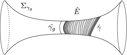
Figure 4: The covering $\Sigma_{\gamma_{g}}$

For $k>0$ we denote by $\tilde{F_{k}}$ the set $\bigcup_{-k\leq i\leq k}(\tilde{\gamma_{i}}\cup\tilde{E_{i}})\setminus\widetilde{\gamma_{-k}}$. The $\tilde{F_{k}}$ form an exhaustive sequence of open disks in $\tilde{F}=\bigcup_{i\in G_{c}}(\tilde{\gamma_{i}}\cup\tilde{E_{i}})$, thus in particular $\tilde{F}$ is an open set. As a consequence, $\hat{F}=\hat{E}\cup\hat{\gamma}$ is an open set in $\Sigma_{\gamma_{g}}$, and so is $F=E\cup\gamma$ in $\Sigma$. We claim that the inclusion of $\hat{F}$ in $\Sigma_{\gamma_{g}}$ induces an injective morphism on fundamental groups; to see it take a simple closed curve $\hat{\delta}$ in $\hat{F}$ bounding a disk in $\Sigma_{\gamma_{g}}$; $\hat{\delta}$ lifts to a closed curve $\tilde{\delta}$ in $\mathbb{H}^{2}$ also bounding a disk, but that curve lies in some $\tilde{F_{k}}$ because $\tilde{\delta}$ is compact. Now, $\tilde{F_{k}}$ is a disk, hence the disk bounded by $\tilde{\delta}$ lies in $\tilde{F_{k}}\subset\tilde{F}$ and as a consequence, the disk bounded by $\hat{\delta}$ lies in $\hat{F}$, proving the claim. This claim implies that $\hat{F}$ is either a disk or an annulus. We prove now that it is not a disk: We take a point $\tilde{y}$ in $\tilde{E_{i}}$, with image $\hat{y}$ in $\Sigma_{\gamma_{g}}$. The lift to $\mathbb{H}^{2}$ at $\tilde{y}$ of a loop based at $\hat{y}$ and freely homotopic to $\gamma_{g}$ gives a path whose other endpoint $\tilde{y^{\prime}}$ lies in $\widetilde{E_{i+1}}$. We link $\tilde{y}$ and $\tilde{y^{\prime}}$ by a path $\tilde{\eta}$ in the disk $\tilde{E_{i}}\cup\widetilde{\gamma_{i+1}}\cup\widetilde{E_{i+1}}$. Note that $\tilde{\eta}$ projects to a loop $\hat{\eta}$ in $\hat{F}$ which is not null-homotopic. Hence $\hat{F}$ is an open annulus, and as such, it contains a compact annulus with PL boundary, which projects to $\Sigma$, as a subset of $F=E\cup\gamma$. Since the projection of the boundary of the above annulus can be seen as a pair of PL closed curves homotopic to $\gamma_{g}$, which is simple, we can erase their self-intersections if any, and also the intersections they may have with each other; moreover these erasures can be performed in $F$, so they cobound in $F$ an annulus whose boundary components (as curves) are homotopic to $\gamma_{g}$. $\diamondsuit$

The following corollary follows:

Corollary 3.5.

Let $\cal T$ be a topological lamination on a surface $\Sigma$ containing a non-compact leaf $\gamma$ homotopic to a simple closed curve. Then there is a lamination ${\cal T}_{\delta}$ sharing with $\cal T$ the same leaves except $\gamma$, which has been replaced by a simple closed curve $\delta$ homotopic to $\gamma$.

Proof. The fact that $\cal T$ is carried by a train track implies that the closed curve $\gamma$ is homotopic to is essential in $\Sigma$, hence is freely homotopic to a simple closed geodesic. Under these conditions, Lemma 3.4 says that there is in the complement of ${\cal T}\setminus\gamma$ in $\Sigma$, an annulus containing a simple closed curve $\delta$ homotopic to $\gamma$. Hence ${\cal T_{\delta}}=({\cal T}\setminus\gamma)\cup\delta$ is a lamination as desired . $\diamondsuit$

Corollary 3.5 allows the following convention:

Convention 3.6.

In a topological lamination we always replace a two-way infinite curve homotopic to a closed one avoiding the rest of the lamination, by the closed one.

Note that for geodesics this point of view is natural, since on a hyperbolic surface, there can be only one geodesic homotopic to a curve and it is closed if the curve is closed. With this convention, the combination of Corollary 3.2 and Proposition 3.3 gives one direction of the equivalence between Definitions 1 and 2.

4 A Geodesic Lamination is a Topological Lamination

It suffices to prove it for connected geodesic laminations, and in this section $\cal L$ denotes such a lamination. We begin by remarking that $\cal L$ contains no leaf joining two punctures. This can be seen as follows: Suppose $\cal L$ contains such a (necessarily isolated) leaf $\ell$. We can write $\cal L=({\cal L}\setminus\ell)\cup\ell$; however a geodesic joining two punctures is a closed set, and so is ${\cal L}\setminus\ell$, so $\cal L$ is not connected.

To describe how geodesics in a complementary region of a geodesic lamination behave we need the notion of spike. A spike is a surface isometric to the connected closed region of bounded area in $\mathbb{H}^{2}$, delimited by two disjoint complete geodesics sharing an endpoint, and an arc $a$ meeting each of them along one of its endpoints. The arc $a$ is called the base of the spike. An open spike is the interior of a spike union the interior of its base. (See Figure 5)

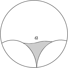
Figure 5: A spike in $\mathbb{H}^{2}$, with interior shaded

To work in fibered neighborhoods of train tracks we also need the notion of box. A box $D$ in a fibered neighborhood of a train track is a union of subarcs of the fibers which forms an embedded closed disk, such that its frontier $\partial D$ consists of a pair of disjoint subarcs of two (not necessarily distinct) fibers, the small sides of $D$, union a pair of piecewise $C^{1}$ disjoint arcs everywhere transverse to the fibers, the large sides of $D$ (see Figure 6).

Let $N_{\varepsilon}({\cal L})$ be the set of points of $\Sigma$ at distance no more than $\varepsilon$ from $\cal L$. Then $N_{\varepsilon}({\cal L})$ is the union (in a non-unique way) of a compact topological surface embedded in $\Sigma$ and finitely many neighborhoods of spikes. It is known that $N_{\varepsilon}({\cal L})$ can be decomposed as a disjoint union of piecewise $C^{1}$ arcs making $N_{\varepsilon}({\cal L})$ a fibered neighborhood of $\cal L$ [1, 5]. Also, collapsing each fiber to one point yields a corresponding graph $\Gamma(\varepsilon,{\cal L})$, that embeds in $\Sigma$ with edges $C^{1}$-embedded in such a way that the tangent space at each vertex is well-defined; moreover if $\varepsilon$ is small enough the connected components of $\Sigma\setminus\Gamma(\varepsilon,{\cal L})$ satisfy the conditions in order that $\Gamma(\varepsilon,{\cal L})$ is a train track [1, Prop. 8.9.2]. The boundary components of $N_{\varepsilon}({\cal L})$ are differentiable everywhere except at finitely many points called cusps. Adequately stretching the fibers in small neighborhoods of cusps makes $N_{\varepsilon}(\cal L)$ into a new fibered neighborhood $N_{1}$ of $\cal L$ such that no two cusps lie in the same fiber; we call the corresponding graph obtained by collapsing each fiber to one point, $\Gamma_{1}$. After ambient isotopy the graph $\Gamma_{1}$ can be embedded in such a way that $N_{1}$ is a regular neighborhood of it, and that $\Gamma_{1}$ strongly carries $\cal L$. Note that as a graph, $\Gamma_{1}$ is trivalent.

Suppose there exists a simple geodesic $\gamma_{g}$ in the complement of $\cal L$ homotopic to a path on $\Gamma_{1}$. We have:

Lemma 4.1.

The geodesic $\gamma_{g}$ decomposes as a geodesic arc union two disjoint geodesic one-way infinite curves $\gamma_{g}^{-}$ and $\gamma_{g}^{+}$ in $N_{1}$, each contained in a spike bounded by boundary leaves of $\cal L$. Accordingly, the path on $\Gamma_{1}$ homotopic to $\gamma_{g}$ decomposes as a finite path union two one-way infinite subpaths of paths homotopic to boundary leaves of $\cal L$.

Proof. The first assertion is a straightforward consequence of the structure theorem about geodesic laminations [14, Th. 4.2.8]: Whatever the direction chosen on $\gamma_{g}$, $\gamma_{g}$ eventually enters an open spike bounded by two boundary leaves of $\cal L$. Moreover, when these spikes become sufficiently thin (i.e. the pieces of fibers of $N_{1}$ joining the two boundary leaves become sufficiently short), they are subsets of $N_{\varepsilon}({\cal L})\subset N_{1}$, because of $N_{\varepsilon}({\cal L})$’s definition. Hence $\gamma_{g}^{-}$ and $\gamma_{g}^{+}$ can be taken to be subsets of $N_{1}$. The second assertion is an obvious consequence of the first one. $\diamondsuit$

There is no reason $\gamma_{g}$ should be entirely contained in $N_{1}$. However:

Lemma 4.2.

The path $\gamma$ on $\Gamma_{1}$ homotopic to $\gamma_{g}$ can be moved by a homotopy in such a way that it becomes a simple curve $\gamma\subset N_{1}$, disjoint from $\cal L$, and transverse to the fibers of $N_{1}$.

Proof. The neighborhood $N_{1}$ can be seen as a union of boxes, one box for each edge of $\Gamma_{1}$.

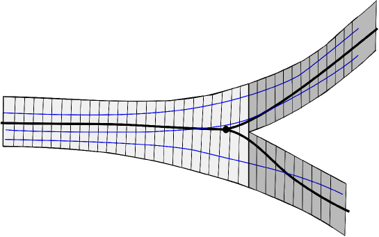
Figure 6: A part of $N_{1}$, formed by the union of three boxes.

We fix in $\gamma_{g}$ two one-way infinite geodesic curves $\gamma_{g}^{-}$ and $\gamma_{g}^{+}$, whose existence is asserted in Lemma 4.1. Up to taking them shorter we can assume that $\gamma_{g}^{-}$ and $\gamma_{g}^{+}$ have their endpoints on sides of two boxes $R^{-}$ and $R^{+}$ respectively, in such a way that they can be prolonged through $R^{-}$ and $R^{+}$. We now prolong, say $\gamma_{g}^{-}$, through $R^{-}$ using a geodesic arc disjoint from the boundary leaves of $\cal L$. We carry on this process of prolonging the path without creating intersections with $\cal L$’s boundary leaves or self-intersections. If at some of the boxes forming $N_{1}$ we had to intersect $\cal L$’s boundary leaves or the already drawn arc to be able to continue, lifting to $\mathbb{H}^{2}$ and applying Lemma 2.1 would give a non-erasable intersection between a lift of $\gamma$ and a lift of a path homotopic to some leaf of $\cal L$, or a non-erasable intersection between two lifts of $\gamma$. This would contradict the hypothesis that $\gamma_{g}$ is simple and misses $\cal L$. Hence we can continue, following the finite path whose existence is asserted in Lemma 4.1. This being done, we meet $R^{+}$ in such a way that we can join the already drawn arc to $\gamma_{g}^{+}$, and this can be done without creating intersections, again thanks to Lemma 2.1. $\diamondsuit$

We can prove now:

Proposition 4.3.

For any connected geodesic lamination $\cal L$, there is a train track carrying it in a maximal way.

Proof. We begin with the neighborhood $N_{1}$, which, as said in the preceding lemma, can be seen as a union of boxes, one box for each edge of $\Gamma_{1}$. Suppose $\gamma_{g}$ is a geodesic in $\Sigma\setminus{\cal L}$ homotopic to a path on $\Gamma_{1}$. We assume first that $\gamma_{g}$ does not end up at a puncture. We denote by $\gamma$ a simple curve in $N_{1}$ homotopic to $\gamma_{g}$ whose existence is proved in Lemma 4.2.

We denote by $\gamma_{g,1}^{-}$ and $\gamma_{g,2}^{-}$ two geodesics in $\cal L$ forming a spike meeting $\gamma$ along a one-way infinite curve. Since the leaves of $\cal L$ and $\gamma$ are transverse to the fibers of $N_{1}$, when we go sufficiently far into the spike we can find in some fiber a subarc $a$ joining $\gamma_{g,1}^{-}$ and $\gamma_{g,2}^{-}$, and meeting $\gamma$ at one point.

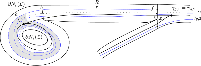
Figure 7: A part of $N_{1}$, where an open spike containing $a$’s interior is shaded. In this example $\gamma_{g,1}^{-}=\gamma_{g,2}^{-}$ spirals around a closed geodesic (not represented).

As a first step, we translate $a$ along $\gamma$ so as to move away from the spike. The translation is possible until the moment we hit a cusp, which is also the intersection point between two small sides of two boxes of $N_{1}$. This eventually happens since none of $\gamma_{g,1}^{-}$ or $\gamma_{g,2}^{-}$ is homotopic to $\gamma$, and this ends step 1. Two boxes share the hit cusp, and we choose the one, $R$, visited by the prolonging of $\gamma$. Then, one of $\gamma_{g,1}^{-}$ or $\gamma_{g,2}^{-}$, say the latter, enters also $R$ together with $\gamma$. In $R$ there is a thinner box $r$ whose one large side is a side of $R$ and the other one is a subarc of $\gamma_{g,2}^{-}$, its small sides being subarcs of $R$’s small sides.

As a second step we translate further through $r$ along $\gamma$, and even further than $r$ provided we do not have to stop at a cusp $x$. However we have to stop some time, ending thus step 2, since, again, $\gamma$ is not homotopic to $\gamma_{g,2}^{-}$. Then, the hit cusp $x$ must be an endpoint of a small side of the box resulting from the translation, in some fiber $f$ of $N_{1}$, as shown in Figure 7. Indeed, if the hit cusp was in the interior of the small side where we stopped translating (see Figure 8), one of the boxes forming $N_{1}$ would not be visited by any leaf of $\cal L$, which is impossible.

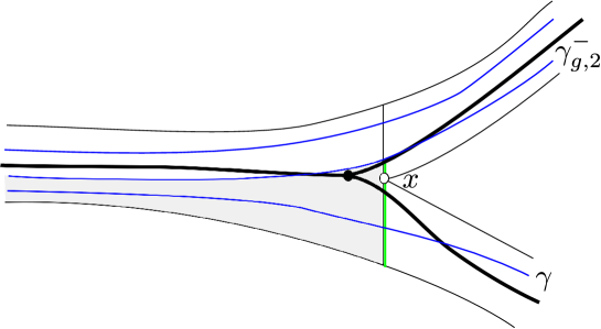
Figure 8: Stopping the translation at a hit with a cusp $x$ in the interior of a box small side.

When this happens, the fiber $f$ necessarily intersects pieces of leaves of $\cal L$, and by compactness of $\cal L$ there is a subarc $c\subset f$ joining $\gamma_{g,2}^{-}$ to another boundary leaf $\gamma_{g,3}^{-}$, such that $c$ contains no hit with any leaf of $\cal L$ other than $\gamma_{g,2}^{-}$ and $\gamma_{g,3}^{-}$.

We begin then Step 3; we are in a situation similar to the one we had at the beginning of step 1, when we started moving $a$ away from the spike, with now the subarc $c$, that we can translate following $\gamma$ until we hit again a cusp, putting an end to this step. If the cusp $y$ we eventually hit lies between the hit of $\gamma_{g,2}^{-}$ and the one of $\gamma$ in the fiber containing $y$, there exists in $N_{1}$ an arc $\delta$ transverse to the fibers, joining $x$ and $y$, and disjoint from $\cal L$; $\delta$ always exists because no two cusps lie on the same fiber. If $y$ does not lie between the hit of $\gamma_{g,2}^{-}$ and the one of $\gamma$, we are in the same situation as at the beginning of step 2, and we can proceed step 4 in a way similar to step 2.

If this process never stops, then $\gamma_{g,2}^{-}$ is homotopic to $\gamma$, and this contradicts the hypothesis. Hence for some $k\geq 1$, at step $2k+1$ we reach a situation where the hit cusp $y$ lies between the hit of $\gamma_{g,2}^{-}$ and that of $\gamma$ in the fiber containing $y$. We conclude that there is always an arc $\delta$ transverse to the fibers, missing $\cal L$, and joining $x$ to another cusp $y$.

We slit open $N_{1}$ along $\delta$, i.e. we remove from $N_{1}$ the interior of a thin box neighborhood of $\delta$ missing $\cal L$, to get a fibered neighborhood $N_{2}$ containing $\cal L$, in such a way that $\cal L$ is transverse to the fibers. After smoothing, $\partial N_{2}$ has two fewer cusps than $N_{1}$.

We repeat on $N_{2}$ the process undergone for $N_{1}$, and so on. Since the number of cusps decreases, we eventually reach a situation where, after $n$ slitting open operations, the interior of the obtained fibered neighborhood $N_{n}$ of $\cal L$ contains no more arcs transverse to all the fibers, joining two punctures, and missing $\cal L$. If the corresponding train track $\Gamma_{n}$ had a path homotopic to some geodesic in $\Sigma\setminus{\cal L}$, thanks to Lemmas 4.1 and 4.2 we would obtain a simple curve $\gamma$ in $N_{n}$ whose existence would imply the existence of an arc as above, and this is impossible. Hence the carrying of $\cal L$ by $\Gamma_{n}$ is maximal.

When $\gamma_{g}$ ends up at a puncture (necessarily only) in one direction, the situation is easier: In the direction where the associated path $\gamma$ given by Lemma 4.2 does not end up at a puncture it enters a spike bounded by two boundary leaves $\gamma_{g,1}^{-}$ and $\gamma_{g,2}^{-}$ of $\cal L$, so the beginning of the above argument applies, and in the other direction $\gamma$ runs only along finitely many edges. $\diamondsuit$

Proposition 4.3 ends the proof of the equivalence of Definitions 1 and 2 up to isotopy.

5 Moving Topological Laminations into their Carrier Train Track Neighborhoods

In this section we relax the dependency on the embedding surface, by proving that a weakly carried lamination satisfies, up to ambient isotopy, the first requirement for being strongly carried, that is, to be contained in a regular neighborhood of the carrying train track.

We begin with a lemma about the leaves ending up at a puncture:

Lemma 5.1.

Let $\cal T$ be a topological lamination containing curves ending up at punctures, then there is an ambient isotopy sending $\cal T$ to a topological lamination such that all the leaves ending up at punctures are PL in a neighborhood of the punctures.

Proof. The set of leaves ending up at a puncture is finite. For each puncture and each leaf ending up at it, we choose a one-way infinite curve ending up at that puncture in that leaf. According to Lemma 3.1 there is an ambient isotopy bringing each of these one-way infinite curves to a PL curve while fixing the rest of the lamination. Composing these finitely many ambient isotopies makes all the leaves ending up at punctures, PL near the punctures. $\diamondsuit$

An embedded graph in $\Sigma$ (not necessarily a train track) fills $\Sigma$ if each of the connected components of the complement of the graph is either a disk or a once punctured disk. For a filling graph $G$, its dual graph in $\Sigma$ is defined as follows: In each disk component of $\Sigma\setminus G$ we choose a point. These points and the punctures in the once punctured disk components of $\Sigma\setminus G$ are joined with each other by PL simple curves, actually arcs or one-way infinite curves with pairwise disjoint interiors in $\Sigma$, in such a way that each pair of (not necessarily distinct) components sharing an edge of $\Gamma$ are joined, and the joining curve meets $\Gamma$ in only one point, in that edge. The resulting embedded graph $G^{d}$ is called a graph dual to $G$. (See Figure 9)

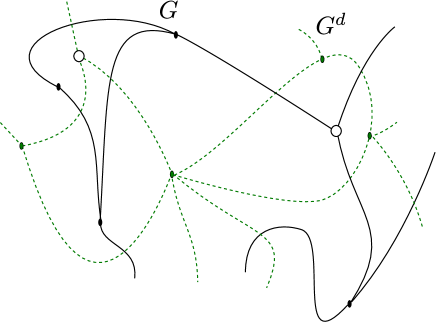
Figure 9: Part of a graph $G$ and of its dual $G^{d}$. Solid lines represent $G$’s edges, narrow dashed ones, $G^{d}$’s edges, and small circles, punctures of $\Sigma$ (there are two of them).

Since all the components of $\Sigma\setminus G$ are disks or once punctured disks, any two dual graphs are isotopic, hence ambient isotopic, so $G^{d}$ is essentially unique. We have:

Remark 5.2.

Let $G$ be a filling graph in $\Sigma$. Then $G$ is the dual graph of $G^{d}$.

Proof. By construction, the connected components of $\Sigma\setminus G^{d}$ satisfy the same topological constraints as those of $\Sigma\setminus G$, with the difference that a disk component of $\Sigma\setminus G^{d}$ contains a preferred point in it, that is, the (unique) vertex of $G$ whose adjacent edges hit the frontier of this component. And the situation is similar for the once punctured disks of $\Sigma\setminus G^{d}$. Thus we can take these points and punctures as the vertices of the dual of $G^{d}$, these are actually exactly the vertices of $G$. For the edges of $G^{d}$’s dual we just take the edges of $G$. $\diamondsuit$

The following corollary is the core of the proof of Lemma 5.6:

Corollary 5.3.

Let $G$ be a filling graph in $\Sigma$. Then there is a set of neighborhoods of $G^{d}$’s vertices in $\Sigma$ such that the complement of the union of these neighborhood interiors is a regular neighborhood of $G$.

Proof. This type of result is classical in PL Topology. We take disjoint closed PL neighborhoods missing $G$ of each of $G^{d}$’s vertices, each being a PL disk or once punctured disk according to whether the considered vertex lies in $\Sigma$ or is a puncture, in such a way that if the frontier of the component of $\Sigma\setminus G$ the vertex lies in contains punctures, the frontier of the neighborhood contains the same punctures. The complement in $\Sigma$ of the union of these neighborhood interiors is a PL subsurface of $\Sigma$, which collapses onto $G$, so it is a regular neighborhood of $G$. $\diamondsuit$

We need one more graph associated to $G$, which is built using both $G$ and $G^{d}$. A puncture graph of an embedded graph $G$ is a graph $\Lambda_{G}$, whose vertices are the punctures and those vertices of $G^{d}$ whose neighborhood frontiers contain punctures, and the edges are arcs whose interiors lie in $\Sigma\setminus G$, joining each such vertex to the punctures on its neighborhood frontier. The edges of $\Lambda_{\Gamma}$ can be taken PL since by Lemma 5.1 the frontier leaves are PL near the punctures. Again, up to ambient isotopy $\Lambda_{G}$ is unique.

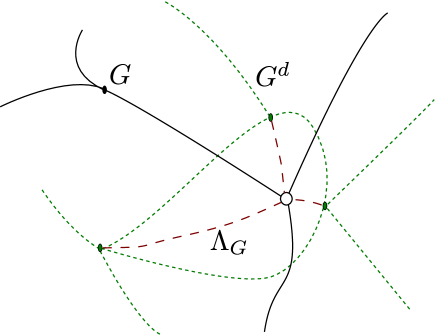
Figure 10: part of a puncture graph $\Lambda_{G}$. Its edges are represented as wide dashed lines

For connected train tracks we have:

Lemma 5.4.

Let $\Gamma$ be a connected train track. The vertices of $\Gamma$ which are not punctures all lie in the same connected component of the complement of $\Gamma$’s puncture graph $\Lambda_{\Gamma}$.

Proof. Let $\Lambda_{\Gamma}$ be the puncture graph of $\Gamma$ in $\Sigma$. Any path joining two vertices of $\Gamma$ lying in two distinct components of $\Sigma\setminus\Lambda_{\Gamma}$ would have to contain a puncture vertex in its interior, so it is would not be admissible, but this contradicts the hypothesis that $\Gamma$ is connected. $\diamondsuit$

Let $\cal T$ be a topological lamination carried by a train track $\Gamma$. To each frontier leaf of $\cal T$ there corresponds one two-way infinite path on $\Gamma$, so to each complementary region $E$ of $\cal T$ we associate the set of paths homotopic to its frontier leaves, and call these paths the frontier paths for $E$. We lift the frontier paths for $E$ to $\mathbb{H}^{2}$ through $p$, in such a way that their endpoints coincide with the endpoints of the frontier components of a disk $\tilde{E}\subset\mathbb{H}^{2}$ over $E$. Then, the union of these frontier paths’ lifts delimit regions, lying over connected components of $\Sigma\setminus\Gamma$ that we call components of $\Sigma\setminus\Gamma$ associated to $E$, since the set they form does not depend on the choice of $\tilde{E}$ over $E$. We have:

Lemma 5.5.

Let $\cal T$ be a topological lamination in $\Sigma$ weakly carried by a connected train track $\Gamma$ which fills $\Sigma$. Then $\Gamma^{d}$ is isotopic to an embedded graph $\Delta$ having one vertex in each component of $\Sigma\setminus\Gamma$ associated to $E$, where $E$ runs through the complementary regions of $\cal T$, in such a way that $\Lambda_{\Delta}\subset(\Sigma\setminus{\cal T})$.

Proof. Given a complementary region $E$, we choose in it one point for each disk component $e$ of $\Sigma\setminus\Gamma$ associated to $E$, if $e\cap E\neq\emptyset$ the point for $e$ is taken in $e\cap E$. As for the once punctured disk components, we take their punctures. We mark each point according to the vertex of the dual graph $\Gamma^{d}$ it corresponds to, including the puncture vertices. We denote by $V_{E}$ the set thus obtained, and by $V$ the union of the $V_{E}$ where $E$ runs through the complementary regions of $\cal T$. For each $E$ we slide each non-puncture vertex of the puncture graph of $\Gamma$, $\Lambda_{\Gamma}$, onto the point of $V_{E}$ it corresponds to, in such a way that the edges of $\Lambda_{\Gamma}$ can be moved rel endpoints so as to lie in the union of ${\cal T}^{\prime}s$ complementary regions. These isotopies can be obtained by projecting to $\Sigma$ isotopies in $\mathbb{H}^{2}$ for chosen components of the inverse images by $p$ of $\Lambda_{\Gamma}$ and $E$. The obtained graph is isotopic (hence ambient isotopic) to $\Lambda_{\Gamma}$. Now, a vertex $v$ of $\Gamma^{d}$ which is neither a puncture nor a vertex of $\Lambda_{\Gamma}$ lies in a connected component $e$ of $\Sigma\setminus\Gamma$ whose frontier contains only non-puncture vertices of $\Gamma$, so according to Lemma 5.4 it lies in the same connected component of $\Sigma\setminus\Lambda_{\Gamma}$ as $\Gamma$’s non-puncture vertices. We slide $v$ in $\Sigma\setminus\Lambda_{\Gamma}$ onto its corresponding point in $V$, as follows. There is a complementary region $E$ to which $e$ is associated, and a connected component $\tilde{E}$ over $E$ is delimited by lifts of curves of $\cal T$ (finitely many if $E$ is puncture free). We call $\tilde{F}_{E}$ the set of lifts of frontier paths for $E$ with same endpoints. The latter paths determine disks in $\mathbb{H}^{2}$ over the components of $\Sigma\setminus\Gamma$ associated to $E$, including $e$, and we take one, $\tilde{e}$, over $e$ (if $E$ is puncture free $\tilde{e}$ is unique).

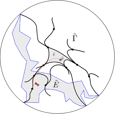
Figure 11: Here $\tilde{e}\cap\tilde{E}=\emptyset$. Four paths in $\tilde{F}_{E}$ determine $\tilde{e}$; a subpath of one of them is projected to $\Sigma$ in order to slide $v$ into $E$.

This disk $\tilde{e}$ is relatively compact because $e$ is, so the closure of $\tilde{e}$ is a compact disk. If $e\cap E\neq\emptyset$ we slide $v$ onto its corresponding point in $E$ without exiting $e$. If $e\cap E=\emptyset$, then $\tilde{e}\cap\tilde{E}=\emptyset$ too, but there is at least one path in $\tilde{F}_{E}$ among those determining $\tilde{e}$ which meets $\tilde{E}$; see Figure 11. We use the image by $p$ of a subpath of it to slide $v$ onto its corresponding point in $E$; note that since $e$ and $E$ are open sets in $\Sigma$ and a frontier path is homotopic to a simple curve (actually a leaf of $\cal T$), the sliding can be made along an arc. Any edge of $\Gamma^{d}$ met during the sliding is dragged along. In this way we obtain from $\Gamma^{d}$ an embedded isotopic graph $\Delta$ with $V$ as set of vertices and such that $\Lambda_{\Delta}\subset(\Sigma\setminus{\cal T})$, as wished. $\diamondsuit$

The following lemma gives the desired result for a lamination carried by a filling train track.

Lemma 5.6.

Let $\cal T$ be a topological lamination in $\Sigma$ weakly carried by a connected train track $\Gamma$ which fills $\Sigma$. Then there is an ambient isotopy of $\Sigma$ sending $\cal T$ to a topological lamination contained in a regular neighborhood of $\Gamma$, in such a way that $\cal T$ is carried by $\Gamma$ inside this neighborhood (i.e. the homotopies deforming $\cal T$’s curves to paths on $\Gamma$ are homotopies in the neighborhood).

Proof. We start with a graph $\Delta$ isotopic to $\Gamma^{d}$ as constructed in the proof of Lemma 5.5. Then in each complementary region $E$, for each vertex $v$ of $\Delta$ in $E$ which is not a vertex of $\Lambda_{\Delta}$, we choose a PL closed neighborhood of $v$, and we choose also a regular neighborhood of $\Lambda_{\Delta}$ in $\Sigma\setminus{\cal T}$. We denote by $N(V)$ the union of all these neighborhoods. Since $\Delta$ is isotopic to $\Gamma^{d}$, by Remark 5.2 the dual graph $\Delta^{d}$ is istopic to $\Gamma$, and we can make $\Delta^{d}$’s edges $C^{1}$, in such a way that the tangent space at each vertex is well-defined and compatible with the one at the corresponding vertex of $\Gamma$. By Corollary 5.3 the complement $N^{\prime}$ of the interior of $N(V)$ is a regular neighborhood of $\Delta^{d}$, such that, by construction $\cal T$ is entirely contained in the interior of $N^{\prime}$. By construction too, all homotopies from $\cal T$’s curves to paths on $\Delta^{d}$ can be performed in $N^{\prime}$. An ambient isotopy taking $\Delta^{d}$ to $\Gamma$ takes $\cal T$ to a topological lamination entirely contained in a neighborhood of $\Gamma$. $\diamondsuit$

To settle the general case we need some more technical results.

Lemma 5.7.

Let $\Sigma_{\gamma}$ be the covering space of $\Sigma$ corresponding to the cyclic group generated by the homotopy class of an essential simple closed curve $\gamma$. Then for every complementary region of $\cal T$, each component $\hat{E}$ over $E$ is either a disk or an annulus.

Proof. As in Lemma 3.4’s proof, the fundamental group of $\Sigma$ is considered at a point $x\in\gamma$, so that the covering space $\Sigma_{\gamma}$ corresponding to the cyclic group generated by the homotopy class of $\gamma$ is an annulus, and the homotopy class of the lift $\hat{\gamma}$ of $\gamma$ to $\Sigma_{\gamma}$ at a point $\hat{x}$ over $x$ generates the fundamental group of $\Sigma_{\gamma}$. Now let $E$ be a complementary region of $\cal T$ and $\hat{E}$ a component over $E$ in $\Sigma_{\gamma}$. The inclusion of $\hat{E}$ in $\Sigma_{\gamma}$ induces an injective morphism on fundamental groups, for if not, there should be a simple closed curve in $\hat{E}$ bounding a disk in $\Sigma_{\gamma}$ but not in $\hat{E}$. But such a disk would contain at least a lift of one of $E$’s frontier leaves, which is impossible, so $\hat{E}$ is a disk or an annulus. $\diamondsuit$

Lemma 5.8.

Let $\cal T$ be a topological lamination, and $\gamma_{c}$ an essential PL simple closed curve in $\Sigma$ not homotopic to any leaf of $\cal T$. Suppose that every leaf of $\cal T$ can be moved away from $\gamma_{c}$. Then there is a PL simple closed curve in $\Sigma\setminus{\cal T}$ homotopic to $\gamma_{c}$.

Proof. Thanks to Convention 3.6 and Proposition 3.3, there is a geodesic lamination $\cal L$ curve-by-curve isotopic to $\cal T$. Let $\gamma_{g}$ be the geodesic homotopic to $\gamma_{c}$. Since $\gamma_{g}$ does not belong to $\cal L$ any intersection between $\cal L$ and $\gamma_{g}$ would have to be a transverse one, but if $\cal L$ intersected $\gamma_{g}$, no homotopy on those of $\cal L$’s leaves hitting $\gamma_{g}$ transversally could give curves missing $\gamma_{g}$, hence $\gamma_{c}$. Thus $\gamma_{g}$ lies in some complementary region $D$ of $\cal L$, and we denote by $E$ the corresponding complementary region of $\cal T$. As in Lemma 3.4, $\Sigma_{\gamma_{g}}$ denotes the covering space of $\Sigma$ corresponding to the homotopy class of $\gamma_{g}$ at a point $x$ chosen as base point for the fundamental group. A point $\hat{x}$ is chosen over $x$ and $\hat{\gamma_{g}}$ denotes the lift at $\hat{x}$ of $\gamma_{g}$. In $\Sigma_{\gamma_{g}}$, the component $\hat{D}$ over $D$ is either a disk or an annulus, by Lemma 5.7, hence it is an annulus because it contains $\hat{\gamma_{g}}$. We take also a component $\tilde{D}$ over $D$ in $\mathbb{H}^{2}$, and denote by $\tilde{\gamma_{g}}$ a curve over $\hat{\gamma_{g}}$ in $\tilde{D}$. We consider the component $\tilde{E}$ of $p^{-1}(E)$ in $\mathbb{H}^{2}$ with the same frontier component endpoints on the circle at infinity as $\tilde{D}$, and $\hat{E}$ its projection to $\Sigma_{\gamma_{g}}$. Like $\hat{D}$, $\hat{E}$ is either a disk or an annulus. If the geodesic $\tilde{\gamma_{g}}$ shares one endpoint with another leaf of $\cal L$, both are necessarily frontier leaves of $\cal L$, but this contradicts the hypothesis, so no lift of a leaf of $\cal L$, hence of $\cal T$, shares an endpoint with $\tilde{\gamma_{g}}$. Now, $E$ has finitely many frontier leaves, and by uniform continuity the lift to $\mathbb{H}^{2}$ of each frontier component of a complementary region of $\cal T$, is contained in the $k$-neighborhood of the lift having the same endpoints of a frontier leaf of $D$, for some $k>0$. Let $K$ be the maximum of all the $k$ over the frontier leaves of $E$. Since each of the frontier leaves of $E$ has its lifts in $\mathbb{H}^{2}$ at distance no more than $K$ from the lift of the frontier component of $D$ sharing the same endpoints, and no lift of a leaf of $\cal T$ or $\cal L$ shares an endpoint with $\tilde{\gamma_{g}}$, only finitely many of $\tilde{E}$’s frontier components hit $\tilde{\gamma_{g}}$. These frontier components are ambient isotopic in $\mathbb{H}^{2}$ to the corresponding frontier components of $\tilde{D}$, and these ambient isotopies bring $\tilde{\gamma_{g}}$ to a curve $\tilde{\gamma}$ sharing its endpoints with $\tilde{\gamma_{g}}$ and contained in $\tilde{E}$. Note that these ambient isotopies can be undergone in $K$-neighborhoods of the involved frontier components of $\tilde{D}$, so that if we take in $\mathbb{H}^{2}$ a (Euclidean) disk centered at $0$ and of (Euclidean) radius $r<1$ sufficiently close to 1, no point of $\tilde{\gamma_{g}}$ outside that disk is contained in any of the above $K$-neighborhoods. In other words the ambient isotopies fix the two subarcs of $\tilde{\gamma_{g}}$ outside the disk. Thus, there is a compact subarc $a$ of $\tilde{\gamma_{g}}$ in $\mathbb{H}^{2}$ such that the above ambient isotopies induce a homotopy rel endpoints from $a$ to another arc $a^{\prime}$ in $\mathbb{H}^{2}$, and by compactness the homotopy is uniformly continuous, so $a^{\prime}$ can be joined to $\tilde{\gamma_{g}}$’s endpoints by the two subarcs of $\tilde{\gamma_{g}}$ outside the disk, to give a curve $\gamma^{\prime}\subset\tilde{E}$ homotopic to $\tilde{\gamma_{g}}$. Then $\gamma^{\prime}$ projects to $\hat{E}\subset\Sigma_{\gamma_{g}}$ as a curve $\hat{\gamma^{\prime}}$ (not necessarily simple or PL, but) homotopic to $\hat{\gamma_{g}}$, hence $\hat{E}$ cannot be a disk, so by Lemma 5.7 it is an annulus . We can then end the proof as in Lemma 3.4, to obtain a PL simple closed curve in $E$ homotopic to $\gamma_{g}$, hence $\gamma_{c}$. $\diamondsuit$

We have the following corollary:

Corollary 5.9.

Let $\cal T$ be a topological lamination in $\Sigma$ weakly carried by a connected train track $\Gamma$ which does not fill $\Sigma$, and let $N$ be a regular neighborhood of $\Gamma$. Then there is an ambient isotopy bringing $\cal T$ onto a topological lamination none of whose leaves intersects a component of $\Sigma\setminus N$ which is neither a disk nor a once punctured disk.

Proof. Let $\Sigma_{0}$ be a component of $\Sigma\setminus N$ which is neither a disk nor a once punctured disk, and $\gamma_{c}$ a compact frontier component of $\Sigma_{0}$. Then $\gamma_{c}$ is essential, and the leaves of $\cal T$ can be moved off $\gamma_{c}$ since they are homotopic to paths on $\Gamma\subset N$. If $\gamma_{c}$ is homotopic to a (necessarily compact) leaf of $\cal T$, an ambient isotopy given by [16, Th. 2.1] brings the leaf onto $\gamma_{c}$. Now $\gamma_{c}$ being compact, it is a frontier leaf, and it is isolated from at least one side because it lies on $\partial N$. We use then a collar neighborhood of $\gamma_{c}$ in the complementary region it is a frontier component of, to push $\gamma_{c}$ into $N$’s interior by an ambient isotopy. If $\gamma_{c}$ is not homotopic to a leaf of $\cal T$, we use Lemma 5.8 to obtain a simple closed curve $\delta$ in some complementary region of $\cal T$, and again, an ambient isotopy from $\delta$ to $\gamma_{c}$ brings $\cal T$ to a lamination avoiding $\gamma_{c}$. We perform the same operation for each of $\Sigma_{0}$’s compact frontier components, taking care that the isotopies used leave fixed the components already missing $\cal T$, until the lamination obtained misses all the compact frontier components of $\Sigma_{0}$. A non-compact frontier component, if any, joins two punctures, and is easily seen to be homotopic, hence ambient isotopic to a simple curve [16] in $\Sigma\setminus\cal T$ joining the same two punctures (obvious on the universal covering), so here too we can move $\cal T$ off such a component by an ambient isotopy. Now, the leaves are connected and meet $\Sigma\setminus\Sigma_{0}$, so since they miss its frontier they miss $\Sigma_{0}$ too. We repeat this process with all the components of $\Sigma\setminus N$ as with $\Sigma_{0}$. $\diamondsuit$

We can now prove the general result about deforming laminations into given regular neighborhoods of their carrier graphs.

Proposition 5.10.

Let $\cal T$ be a topological lamination in $\Sigma$ weakly carried by a train track $\Gamma$. Then there is an ambient isotopy of $\Sigma$ taking $\cal T$ to a topological lamination contained in a regular neighborhood of $\Gamma$, in such a way that $\cal T$ is carried by $\Gamma$ inside this neighborhood (i.e. the homotopies deforming $\cal T$’s curves to paths on $\Gamma$ are homotopies in the neighborhood).

Proof. First, we suppose $\Gamma$ is connected; let $N$ be a regular neighborhood of it. We already treated in Lemma 5.6 the case where $\Gamma$ fills $\Sigma$, so we now treat the case where some connected components of $\Sigma\setminus N$ are neither disks nor once punctured disks, and we apply Corollary 5.9 to move $\cal T$ away from all these components.

In each component of $\Sigma\setminus N$ we choose a point (which is the puncture if the component is a once punctured disk), and we can define a graph $\Gamma^{d}$ dual to $\Gamma$ as in the case when $\Gamma$ is filling. However, while in the filling case the dual graph is unique up to isotopy in $\Sigma$, this does not hold now, because of the components of $\Gamma\setminus N$ which are neither disks nor once punctured disks, namely because these components have non cyclic fundamental groups, so a given pair of points and/or punctures in the components may be joined to each other by non-homotopic paths. Still, a graph which satisfies the two conditions of being dual to $\Gamma^{d}$, and of missing the closure of these components of $\Gamma\setminus N$, is isotopic to $\Gamma$ (as a graph). As in the proof of Lemma 5.6, in the disk and once punctured disk components of $\Sigma\setminus N$ we take disjoint PL closed disk or once punctured disk neighborhoods of the points chosen above. Then, the complement of the union of their interiors together with the other components of $\Sigma\setminus N$ is a regular neighborhood $N^{\prime}$ of a graph $\Delta^{d}$ dual to $\Gamma^{d}$. Since $\cal T$ misses the components of $\Sigma\setminus\Gamma$ which are neither disks nor once punctured disks, it is entirely contained in $N^{\prime}$, and carried by $\Delta^{d}$, as in the proof Lemma 5.6.

Next, when $\Gamma$ is the union of (finitely many) connected components, each carrying one sub-lamination of $\cal T$, two complementary regions of these sub-laminations are either nested or disjoint. In particular, we can drag each connected component of $\Gamma$ into the innermost complementary region containing the sub-lamination it carries, without creating intersections. Note also that lifts of boundary leaves to $\mathbb{H}^{2}$ do not accumulate at each other, except may be on the circle at infinity. Hence we can apply the above procedure to each connected component of $\Gamma$ in the complementary region it lies in, beginning with the innermost ones. $\diamondsuit$

6 Appendix

In this appendix we prove Lemma 3.1.

Lemma 3.1.

For any simple infinite curve in a surface $\Sigma$, there is an isotopy making it a PL curve. If the curve is a one-way infinite curve ending up at a puncture in a leaf of a topological lamination, the isotopy can be realized by an ambient isotopy avoiding the rest of the lamination.

Proof. We use the following definition: A square-like neighborhood of $x\in\Sigma$ is the image $d$ of an embedding of the square $[-1,1]\times[-1,1]$ into $\Sigma$, such that $(0,0)$ is sent to $x$; we call $x$ the center of $d$ and the image of $[-1,1]\times\{0\}$ its axis.

The first claim we prove is an existence result for square-like neighborhoods:

Claim 0: Let $\gamma$ be an infinite curve and $x$ a point on it. Then there is a square-like PL neighborhood $d$ with center $x$ and axis a subarc of $\gamma$, moreover there is a PL arc in $d$ meeting $\partial d$ only at the axis endpoints.

We can suppose $x=\gamma(0)$, and we take a PL disk neighborhood $d$ of $x$ in $\Sigma$; then $\gamma^{-1}(int(d))$ is an open set in $\mathbb{R}$ which can be written as a (maybe infinite) disjoint union of open intervals, where one of them, J, contains 0. Then the two endpoints $y$ and $y^{\prime}$ of $\gamma(\overline{J})$ lie on $\partial d$, and $d$ can be considered as a square-like neighborhood with center $x$ and axis $\gamma(\overline{J})$. Since the latter set is compact, we can cover it with a finite set of PL disks, and these disks allow us to find a PL arc as we want joining $y$ and $y^{\prime}$ in $d$. This proves Claim 0.

Claim 1: Let $d$ be a square-like neighborhood with center $x$ and axis $\delta$. Assume there is another arc $\delta^{\prime}$ in $d$ joining $y=\delta(-1)$ to $y^{\prime}=\delta(1)$, such that $\delta^{\prime}(0)=\delta(0)=x$, and meeting $\partial d$ only at $y$ and $y^{\prime}$. Then there is an ambient isotopy from $\delta$ to $\delta^{\prime}$, and this isotopy can be taken in such a way that it pointwise fixes $x,\partial d$, and the complement set of $d$.

The proof is an imitation of the first part of the proof of [16, Th. A1]. We denote by $\delta^{\prime}_{y}$ and $\delta^{\prime}_{y^{\prime}}$ the subarcs of $\delta^{\prime}$ joining $x$ to $y$ and $y^{\prime}$ respectively. The arcs $\delta^{\prime}_{y}$ and $\delta^{\prime}_{y^{\prime}}$ together with the two arcs joining $y$ and $y^{\prime}$ in $\partial d$, $\beta$ and $\beta^{\prime}$, form two pairs of circles in $d$, $(\beta\cup\delta,\beta^{\prime}\cup\delta)$ and $(\beta\cup(\delta^{\prime}_{y}\cup\delta^{\prime}_{y^{\prime}}),\beta^{\prime}\cup(\delta^{\prime}_{y}\cup\delta^{\prime}_{y^{\prime}}))$. (See Figure 12)

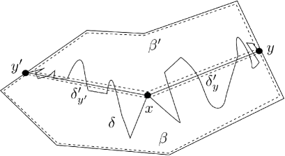
Figure 12: The square-like neighborhood $d$, with $(\beta\cup(\delta^{\prime}_{y}\cup\delta^{\prime}_{y^{\prime}}),\beta^{\prime}\cup(\delta^{\prime}_{y}\cup\delta^{\prime}_{y^{\prime}}))$ represented in dashed lines

Now we apply Schoenflies Theorem to conclude that the first components of these two pairs bound each one disk in $d$, the two disks being homeomorphic, and the same is true for the second components. These two homeomorphisms fix pointwise $\beta$, $\beta^{\prime}$ and $x$, and coincide on $\delta$, so they fit together along $\delta$ to give a homeomorphism $\varphi$ of $d$ onto itself, pointwise fixing $\partial d\cup\{x\}$, so we can apply to it Alexander’s Theorem (also called the Alexander Trick) to conclude that $\varphi$ is isotopic to the identity map of $d$ rel $\partial d\cup\{x\}$, and it sends $\delta$ to $\delta^{\prime}$. This isotopy extends to an ambient isotopy $H$ of $\Sigma$ leaving fixed all the points outside of $d$. This proves Claim 1.

Claim 2: Let $\delta:J=[r,r^{\prime}]\rightarrow\Sigma$ be an arc which is PL near $r$ and $r^{\prime}$. Let $D$ and $D^{\prime}$ be PL disk neighborhoods of $x=\delta(r)$ and $x^{\prime}=\delta(r^{\prime})$ respectively, such that $\delta\cap D$ and $\delta\cap D^{\prime}$ are two PL arcs. Then there is an ambient isotopy fixing $D$ and $D^{\prime}$ from $\delta$ to a PL arc. Moreover, given any fixed neighborhood of $\delta$ and any $\varepsilon>0$, the ambient isotopy can be taken in such a way that it fixes the points outside the neighborhood, and does not move points by more than $\varepsilon>0$ inside. If $\delta$ misses a compact set then the isotopy can be taken so as to avoid it too.

According to [16, Th. A2] applied to the surface with boundary $\Sigma\setminus(int(D)\cup int(D^{\prime}))$, the subarc $\delta^{a}$ of $\delta$ between $\partial D$ and $\partial D^{\prime}$ can be deformed into a PL arc by an ambient isotopy rel endpoints. However it seems difficult to estimate how much points in $\Sigma$ are moved by this isotopy, so we are going to use here this theorem only to conclude that $\delta^{a}$ has a fibered neighborhood $N$ in $\Sigma\setminus(int(D)\cup int(D^{\prime}))$, which can be written as a union of $m$ square-like disk neighborhoods $d_{i}$ satisfying the following four properties:

• $d_{i}$ has diameter no more than $\frac{\varepsilon}{2}$

• $d_{1}\cap D$ and $d_{m}\cap D^{\prime}$ consist each of a subarc in $\partial D$ and $\partial D^{\prime}$ respectively

• $d_{i}\cap d_{j}\neq\emptyset$ iff $|i-j|=1$, in which case this set consists of one fiber of $N$

• $d_{i}\cap\delta^{a}$ is the axis of $d_{i}$

Such $d_{i}$ exist for the following reason: As said above, by [16, Th. A2] there is an ambient isotopy $\phi$ sending $\delta$ to a PL arc with same endpoints, and such a PL arc has a PL product neighborhood $N_{0}\subset(\Sigma\setminus(int(D)\cup int(D^{\prime})))$ any of whose vertical slicings into disks satisfies properties P2 to P4. Now, $\delta$ being compact it admits a finite open covering by disks of diameter no more that $\frac{\varepsilon}{2}$, and the inverse image by $\phi$ of this covering is also an open covering $\cal C$ of $\phi^{-1}(\delta)$, so we can find a smaller product neighborhood $N_{1}$ of $\phi^{-1}(\delta)$ in $N_{0}$ such that it is covered by $\cal C$, and then find a vertical slicing of $N_{1}$ so that each disk produced by this slicing falls in the interior of one of the disks of $\cal C$. The image by $\phi$ of the disks produced by such a slicing give a set of disks $d_{1},\dots,d_{m}$ (in general not PL ones, however) satisfying also property P1.

Now, the arc $\delta^{a}$ meets each arc $d_{i}\cap d_{i+1}$, $i=1,\dots,m-1$ in one point $z_{i}\in int(d_{i}\cap d_{i+1})$, so there is a PL square-like disk $e_{i}$ with center $z_{i}$, with axis a subarc of $d_{i}\cap d_{i+1}$, and contained in $int(d_{i}\cup d_{i+1})$. We put $z_{0}=\partial D\cap\delta^{a}$ and $z_{m}=\partial D^{\prime}\cap\delta^{a}$. Note also that we can suppose the diameter of $e_{i}$ is no more than $\frac{\varepsilon}{2}$. We can now apply Claim 1 to $e_{i}$, $z_{i}$, and $d_{i}\cap d_{i+1}$ seen as a curve, to get an ambient isotopy such that the axis of $e_{i}$ goes to a PL arc containing $z_{i}$ in its interior. Doing this for each $i=1,\dots,m-1$ transforms the $d_{i}$ into a new set of disks $d^{\prime}_{i},i=1,\dots,m$ satisfying properties P1 to P3, and satisfying also P4 with respect to the arc ${\delta^{\prime}}^{a}$ obtained from $\delta^{a}$ after having performed the above $m-1$ ambient isotopies.

Since $z_{0}$ and $z_{m}$ lie in two PL subarcs of $\partial D$ and $\partial D^{\prime}$ respectively, we can find in $d^{\prime}_{1}$ and $d^{\prime}_{m}$ two small PL disks $e_{0}$ and $e_{m}$, such that $\partial d^{\prime}_{1}\cap e_{0}$ and $\partial d^{\prime}_{m}\cap e_{m}$ are two PL arcs containing respectively $z_{0}$ and $z_{m}$ in their interiors. Up to taking PL subdisks of the $e_{i}$ for $i=1,\dots,m-1$, we can assume that $d^{\prime}_{i}\cap e_{i}$ and $d^{\prime}_{i+1}\cap e_{i}$ have the same property with respect to $d^{\prime}_{i}$ and $d^{\prime}_{i+1}$.

Now, for each $i=1,\dots,m$, $({\delta^{\prime}}^{a}\cap int(d^{\prime}_{i}))\setminus(int(e_{i-1})\cup int(e_{i}))$ is a compact set in $int(d^{\prime}_{i})$, so it admits a finite covering by PL disks in $int(d^{\prime}_{i})$. These disks together with $e_{i-1}$ and $e_{i}$ form a finite covering of ${\delta^{\prime}}^{a}\cap d^{\prime}_{i}$, that we can use to link $z_{i-1}$ and $z_{i}$ in $d^{\prime}_{i}$ by a simple PL arc $\delta_{i}$, meeting $\partial d^{\prime}_{i}$ only along $z_{i-1}$ and $z_{i}$. (See Figure 13)

Figure 13: The covering of $\delta^{a}$ by $D$, $D^{\prime}$ (not represented), and $d_{i}$

Applying Claim 1 to $d^{\prime}_{i}$ and ${\delta^{\prime}}^{a}\cap d^{\prime}_{i}$ for each $i$, we get an ambient isotopy fixing $\partial d^{\prime}_{i}$ and sending ${\delta^{\prime}}^{a}\cap d^{\prime}_{i}$ to $\delta_{i}$. This proves Claim 2.

Now we fix an increasing sequence of real numbers $\{r_{n}\}_{n\in\mathbb{Z}}$ or $\{r_{n}\}_{n\in\mathbb{N}}$ according to whether $\gamma$ is two-way infinite or one-way infinite, without accumulation points.

The strategy is to apply inductively Claims 0 and 1 to $\gamma$, taking the indexes of $r_{n}$ alternatively positive and negative in case $\gamma$ is two-way infinite, then Claim 2 to make PL the arcs defined on the intervals $[r_{j},r_{j+1}]$, $j\in\mathbb{Z}$ or $\mathbb{N}$. In the two-way infinite case, we link $k>0$ and the index of $r_{n_{k}}$ at step $k$ by the following formula: $n_{k}=(-1)^{k+1}\left\lfloor\frac{k+1}{2}\right\rfloor$. We start with a curve $\gamma^{(0)}$, obtained by applying Claims 0 and 1 to $\gamma$ and $x^{(0)}=\gamma_{i}(r_{0})$. We denote by $H_{0}$ the resulting ambient isotopy. With the above convention, in any case $n_{1}=1$, and Step 1 consists in applying first Claims 0 and 1 to $\gamma^{(0)}$ and $x^{(1)}=\gamma^{(0)}(r_{1})$, and next Claim 2 to make PL the arc that the resulting curve defines when restricted to $[r_{0},r_{1}]$. The resulting curve is denoted by $\gamma^{(1)}$. When $\gamma$ is two-way infinite (resp. one-way infinite) Step 2 consists in applying Claims 0 and 1 to $\gamma^{(1)}$ and $x^{(2)}=\gamma^{(1)}(r_{-1})$ (resp. $x^{(2)}=\gamma^{(1)}(r_{2})$), then Claim 2 to make PL the arc that the obtained curve defines on $[r_{-1},r_{0}]$ (resp. $[r_{1},r_{2}]$), getting thus a new curve $\gamma^{(2)}$, and so on. With this notation, the arc of Step $k\geq 2$ to be made PL is the subarc of $\gamma^{(k-1)}$ joining $x^{(k-2)}$ and $x^{(k)}$ (resp. $x^{(k-1)}$ and $x^{(k)}$). As for the disk sizes, at Step $k\geq 2$ we require that the disks around the $x^{(k)}$ are pairwise disjoint and have diameters no more than $\frac{1}{2^{k}}$, and also that in the isotopy making PL the arcs joining $x^{(k)}$ and $x^{(k-2)}$ (resp. $x^{(k-1)}$ and $x^{(k)}$), points are not moved by more than $\frac{1}{2^{k}}$. We also ask that the disks at Step $k$ avoid all the arcs already made PL in the preceding steps; this is possible since the union of these arcs is a compact set in $\Sigma$.

Applying the above arguments inductively produces a sequence of ambient isotopies $H_{k}$, $k>0$. For $t\in[0,1]$ fixed, the map $F_{k}(x,t)=H_{k}(.,t)\circ\cdots\circ H_{1}(.,t)\circ H_{0}(.,t)(x)$ is a homeomorphism, and note that because of our choice of disks, the distance in $\Sigma$ between $F_{n}(x,t)$ and $F_{m}(x,t)$, $n<m$ is bounded above by the sum of the diameters of the disks used between Steps $n$ and $m$, that is, $\sum_{j=n}^{m}\frac{1}{2^{j}}<\frac{1}{2^{n-1}}$. This estimation is independent of $x$ and $t$, so the sequence of functions $F_{k}(x,t)$ converges uniformly and the limit is a map $H$ uniformly continuous on $\Sigma\times[0,1]$. In particular the sequence $\{\gamma^{(k)}\}_{k>0}$ converges, and the result is a PL curve $\gamma^{(PL)}$ because after each Step $k$ all the PL arcs built before that step remain fixed in the forthcoming steps. This argument also implies that $\gamma^{(PL)}$ is simple since no self-intersection is created at any step.

We prove now the last assertion. We suppose given a topological lamination carried by a train track. First note that a leaf ending up at a puncture is isolated from both sides, so given any point on the leaf it is always possible to find a neighborhood of the point meeting only the leaf it belongs to. For each puncture we fix a nested sequence $\{N_{i}\}_{i\geq 1}$ of closed once punctured disk neighborhoods with empty intersection in $\Sigma$, such that $N_{i+1}\subset int(N_{i})$. By uniform continuity, given a one-way infinite curve $\gamma$ ending up at a puncture in a leaf of the lamination, for each $i$ there is a least value $r_{i}$ of the parameter such that $\gamma([r_{i},+\infty))\subset N_{i}$. Next, we apply Claims 0 to $\gamma$ and the $\gamma(r_{i})$, using pairwise disjoint square-like neighborhoods, then Claim 1. Since the neighborhoods are disjoint, though they are infinite in number the composition of the ambient isotopies given by Claim 1 is an ambient isotopy of $\Sigma$. Hence we can assume $\gamma$ is PL around the $\gamma(r_{i})$. In this situation, for each $i$, $\gamma([0,r_{i+1}])$ is compact, so for each $i$ we can find a square-like neighborhood $D_{i}$ around $\gamma(r_{i})$, such that $D_{i}\cap\gamma$ is the PL axis of $D_{i}$. Hence the conditions are fulfilled to apply Claim 2 inductively to the $\delta_{i}=\gamma([r_{i},r_{i+1}])$, with disks $D_{i}$ and $D_{i+1}$ around the endpoints. The difference with the general case, is that we can take the disks used in the proof of Claim 2 for $\delta_{i}^{a}=\delta_{i}\setminus(int(D_{i}\cup D_{i+1}))$ disjoint from all the other disks used for $\delta_{j}^{a}$, $j<i$. Hence here too, the non-trivial effect of the ambient isotopies of Claim 2 takes place in pairwise disjoint neighborhoods of the $\delta_{i}^{a}$, hence their (infinite) composition is an ambient isotopy of $\Sigma$. $\diamondsuit$

References

- [1] W. Thurston, The geometry and topology of three-manifolds, Princeton University Lecture Notes, (Electronic Version 1.1 – March 2002) (1980).
- [2] A. Casson, S. Bleiler, Automorphisms of surfaces after Nielsen and Thurston, Vol. 9 of London Mathematical Society Student Texts, Cambridge Univ. Press, 1988.
- [3] F. Bonahon, Geodesic laminations on surfaces, in: Laminations and foliations in dynamics, geometry and topology, Vol. 269 of Contemp. Math., Amer. Math. Soc., 2001, pp. 1–37.
- [4] J. F. Brock, R. D. Canary, Y. N. Minsky, The classification of Kleinian surface groups, II: The ending lamination conjecture, Ann. of Math. 176(1) (2012) 1–140.
- [5] R. Penner, J. Harer, Combinatorics of train tracks, Vol. 125 of Annals of Mathematics Studies, Princeton University Press, 1992.
- [6] A. Hatcher, Measured lamination spaces for surfaces, from the topological viewpoint, Topology Appl. 30 (1) (1988) 63–88.
- [7] X. Zhu, F. Bonahon, The metric space of geodesic laminations on a surface. I, Geom. Topol. 8 (2004) 539–564.
- [8] S. Ferenczi, L. Q. Zamboni, Languages of -interval exchange transformations, Bull. Lond. Math. Soc. 40 (4) (2008) 705–714.
- [9] L.-M. Lopez, P. Narbel, Lamination languages, Ergodic Theory Dynam. Systems 33 (2013) 1813–1863.
- [10] P. Narbel, Bouquets of circles for lamination languages and complexities, RAIRO-Theor. Inf. Appl. 48 (4) (2014) 391–418.
- [11] V. Berthé, V. Delecroix, F. Dolce, D. Perrin, C. Reutnauer, G. Rindone, Return words of linear involutions and fundamental groups, Ergodic Theory Dynam. SystemsTo appear, 2016. doi:10.1017/etds.2015.74.
- [12] S. K. Lando, A. K. Zvonkin, Graphs on surfaces and their applications, Vol. 141 of Encyclopaedia of Mathematical Sciences, Springer-Verlag, Berlin, 2004.
- [13] J. A. Ellis-Monaghan, I. Moffatt, Graphs on Surfaces: Dualities, Polynomials, and Knots, SpringerBriefs in Mathematics, Springer, 2013.
- [14] R. Canary, D. Epstein, P. Green, Notes on notes of Thurston, in: Analytical and geometric aspects of hyperbolic space, Symp. Warwick and Durham 1984, Vol. 111 of London Math. Soc. Lecture Note Ser., Cambridge Univ. Press, Cambridge, 1987, pp. 3–92.
- [15] E. Colin de Verdière, A. de Mesmay, Testing graph isotopy on surfaces, Discrete and Computational Geometry 51 (2014) 171–206.
- [16] D. Epstein, Curves on 2-manifolds and isotopies, Acta Mathematica 115 (1) (1966) 83–107.