The Clauser-Horne-Shimony-Holt inequality in the context of a broad random variable

Abstract

In this work we aim to analyze the Clauser-Horne-Shimony-Holt CHSH inequality strictly in the context of probability theory. In the course of assembling inequality we have to take care not to produce assumptions a priori, that is, physically or intuitively accepted suppositions. Of course, this does not mean that after these considerations, we put the adequate physical conditions suitable and generally accepted in these contexts. This allows us to clearly visualize the possibility of finding a greater inequality than that of CHSH in which it is included. This inequality does not contradict the CHSH inequality. This result is suported by using a robust computational simulation, showing the possibility for obtaining an inequality for quantum mechanics that is not violated and allows random hidden variables without any conflict with Bell’s inequality.

Keywords: Violation of the inequality of CHSH; Axioms of Kolmogorov.

I Introduction

In 1935, A. Einstein, together with B. Podolsky and N. Rosen published an article einstein1935b on quantum mechanics, whose translated title can be described as “can quantum mechanics on the physical reality be considered complete?” Arguing the possibility of ”hidden variances” (random variables) that, if their values were known, a quantum mechanics experiment would no longer be random and would become deterministic, that is, the randomness of the quantum experiment comes from the lack of information of such variables.

In 1964, John S. Bell (in response to the paradox of Einstein, Podolsky and Rosen) published an article Bell1964a in which he developed an inequality involving statistical correlation and, from of the assumption that quantum mechanics would be a statistical theory, one should have a random variable involved with observations. Thus, a variable in which, if it were possible to know its value, the result of the experiment would be completely predictable. Therefore, the lack of predictability of the experiment would be due to ignorance about the value that such variable assumes in the experiment’s performance. By John S. Bell, using the formula obtained by calculating probabilities in the Quantum Mechanics experiment, finds a set of values in which the inequality is violated, and hence concludes the Kolmogorov’s axioms of probability are not sufficient to describe quantum phenomena.

In 1969 J. F. Clauser, M. A. Horne, A. Shimony and R. A. Holt PhysRevLett_23_880 fit the Bell inequality for a viable experiment. In 1982, Aspect, Dalibard and Roger citeulike_679960 conducted an experiment to observe the violation of Clauser-Horne-Shimony-Holt inequality in practice. After performing the experiment, they used the data in the inequality and concluded that this inequality, obtained by means of probabilistic arguments, was violated. It is confirmed, therefore, that the conclusions obtained by John S. Bell about the theory of hidden variables was not possible in the conditions proposed by Einstein, Podolsky and Rosen.

Since then, works that seek to establish a quantum probability or the use of other systems of probability axioms citeulike_3633707 can be found.

The analysis of the probabilistic assumptions of Bell’s arguments is extremely important for modern quantum physics and the consequences of the modern interpretation of the violation of Bell’s inequality for the foundations of quantum mechanics are really relevant from a conceptual and practical reason. Hence, the conditions for deriving this inequality should be carefully checked.

Here the focus of our considerations is to strictly analyze the probabilistic conditions that have been assumed for the demonstration of CHSH inequality. Once the theoretical study of the basic assumptions for the CHSH inequality has been made, it is verified, through simulations, the manner in which the data of the samples should be used for such assumptions to be obeyed. In this way, both population and sample aspects shall be demonstrated.

We will start, in section II, by presenting the experiment and the set of Probability functions associated with it, together with the application of the CHSH inequality, generally found in the literature. Section II and the first part of section X presents what is found in the literature, in the Other sections and the second part of section X are the exclusive results of this work.

After this presentation of the experiment, we present that the proposal of this work is to analyze the inequality, starting by analyzing the question of the hidden variable $\lambda$, in the section III. The conclusions we reach in this section serve as a justification for concentrating only on the random variables $Z_{j}$.

In the section IV and in the section V it is shown that the set of probability functions, which are used in the literature, are consistent (ie it is possible to assign values to the functions of probabilities of $(Z_{1},Z_{2},Z_{3},Z_{4})$ such that one can find marginal probabilities of $(Z_{j},Z_{k})$, with $j\in\{1,2\}$ and $k\in\{3,4\}$). However, this set of probability functions (found in the literature), for certain values of the parameters, leads to a violation of CHSH inequality. We show that this violation only occurs when there is a violation of Kolmogorov’s axioms (that is, the values attributed to the probability functions of $(Z_{1},Z_{2},Z_{3},Z_{4})$ violate the axiom that says the probabilities must be greater than or equal to zero, or violates the axiom which says that the sum of the probabilities must be 1).

In the section VI we have developed a basic inequality, from which both the Bell inequality and the CHSH inequality can be demonstrated. We also show, in the section VII, that from the Bell inequality we can arrive at the CHSH inequality, and the relation between the regions where there is the violation for the Bell and CHSH inequalities.

In section VIII we proposed the use of the conditional probability in the CHSH inequality., we have justified such proposal through the experimental scheme that was found in the literature. We proved that, calculating the expected values, based on the use of conditional probabilities, any possibility of violation from the CHSH inequality disappears.

In section IX it is described the algorithm used in the simulations. In section X, first we have presented how the generated samples are used in the literature, emerging the violation of the CHSH inequality, so we after have presented the proposal of this work of how to use the samples so that any violation of the CHSH inequality disapears and we presented justifications for such use.

Finally, in the section XI we present our conclusions about the modeling of the experiment, as well as the theoretical aspects related to the problem.

II The experiment

In this section we describe and analyze the experiment proposed by Aspect et. al. 1982 citeulike_679960 . The experiment consists of a source that emits entangled pairs of photons with correlated polarizations, which are emitted in opposite directions to two polarizers by the source. Each polarizer is implemented in a way that it acts according to the orientation angle ${\theta}_{1}$ and ${\theta}_{2}$, respectively. The angle ${\theta}_{k}$ provides the vector ${\vec{r}}_{k}=\rm{cos}({\theta}_{k})\cdot\vec{i}+\rm{sin}({\theta}_{k})\cdot\vec{j}$, that represent the orientation of the polarization . Each polarizer record it , if the photon will cross it ($Z_{k}(w)=+1$), or not ($Z_{k}(w)=-1$). We represent $k=1$ for the 1st. photon and $k=2$ for the 2nd photon. The probability of each photon to cross or not the polarizer citeulike_9323624 , it is given by

$${{\mathcal{P}}}_{\dot{Z}_{1,2}}(Z_{1}(w),Z_{2}(w);{\bar{\theta}}_{1,2})=\left\{\begin{array}[]{c}\frac{{\rm{cos}}^{2}({\bar{\theta}}_{1,2})}{2}\Leftarrow(Z_{1}(w),Z_{2}(w))\in C\\ \frac{{\rm{sin}}^{2}({\bar{\theta}}_{1,2})}{2}\Leftarrow(Z_{1}(w),Z_{2}(w))\in\bar{C}\end{array}\right.,\qquad\left\{\begin{array}[]{l}C:=\{(-1,-1),(+1,+1)\}\\ \bar{C}:=\{(-1,+1),(+1,-1)\}\\ \bar{\theta}_{j,k}:=\theta_{k}-\theta_{j}\\ \dot{Z}_{j,k}:=(Z_{j},Z_{k})\end{array}\right.\$$ (7)

where ${\bar{\theta}}_{1,2}={\theta}_{2}-{\theta}_{1}$ (is the angles’ difference from the orientations of the polarizers) and the random variables $Z_{1}$ and $Z_{2}$ are the passage or not for their respective polarizers. In search of determining the $w$ associate to the experiment of measuring the crossing or not of the photons that have been emitted with the polarization property correlated, it will be admitted more two polarizer’s orientations (totalling 4 orientations: $a_{1}$, $a_{2}$, $b_{1}$ and $b_{2}$) and more two measures (totalling 4 random variables: $Z_{1}(w),Z_{2}(w),Z_{3}(w),Z_{4}(w)\in\{-1;+1\}$. Therefore, the experiment was conducted for the same number of times for the polarizers, with the following directions: a) Direction ${\theta}_{1}$ in the polarizer $I$ and ${\theta}_{3}$ in the $III$; b) Direction ${\theta}_{1}$ in the polarizer $I$ and ${\theta}_{4}$ in the $IV$; c) Direction ${\theta}_{2}$ in the polarizer $II$ and ${\theta}_{2}$ in the $III$; d) Direction ${\theta}_{2}$ in the polarizer $II$ and ${\theta}_{4}$ in the $IV$. The demonstration of the inequality citeulike_8683605 ; citeulike_9323624 is based on Statistical arguments. We compared the predictions from the statistics with the results obtained by the Quantum Mechanics. Thus, we omitted the parameters ${\theta}_{j}$ and $w$ (example: $\mathcal{P}_{Z_{j},Z_{k}}(Z_{j}(w),Z_{k}(w);\bar{\theta}_{j,k})\equiv\mathcal{P}_{Z_{j},Z_{k}}(Z_{j},Z_{k})$ or $\mathcal{P}_{Z_{j},Z_{k}}(a,b;\bar{\theta}_{j,k})\equiv\mathcal{P}_{Z_{j},Z_{k}}(a,b)$).

Calculating the expected value of $Z_{1}\cdot Z_{2}-Z_{1}\cdot Z_{4}+Z_{2}\cdot Z_{3}+Z_{2}\cdot Z_{4}$ and observing that $-2\leq Z_{1}\cdot\left(Z_{3}-Z_{4}\right)+Z_{2}\cdot\left(Z_{3}+Z_{4}\right)\leq 2$ is enough to substitute the values, convincing the validity of that inequality, then

$$|Z_{1}\cdot Z_{2}-Z_{1}\cdot Z_{4}+Z_{2}\cdot Z_{3}+Z_{2}\cdot Z_{4}|\leq 2$$

If we multiply both members of the inequality by an amount that is not negative, the inequality remains. Assuming the existence of probability function $\mathcal{P}_{\ddot{Z}}(Z_{1},Z_{2},Z_{3},Z_{4})$ (which, according to the axioms of Kolmogorov Mood_IntroTheoryStats ; magalhaes2006probabilidade , must be greater than or equal to zero for any values $(Z_{1},Z_{2},Z_{3},Z_{4})$, that is, $|\mathcal{P}_{\ddot{Z}}(Z_{1},Z_{2},Z_{3},Z_{4})|=\mathcal{P}_{\ddot{Z}}(Z_{1},Z_{2},Z_{3},Z_{4})$), we have

$$\forall_{(Z_{1},Z_{2},Z_{3},Z_{4})\in\{-1,+1\}^{4}}(|Z_{1}\cdot Z_{2}-Z_{1}\cdot Z_{4}+Z_{2}\cdot Z_{3}+Z_{2}\cdot Z_{4}|\cdot\underbrace{\mathcal{P}_{\ddot{Z}}(Z_{1},Z_{2},Z_{3},Z_{4})}_{=|\mathcal{P}_{\ddot{Z}}(Z_{1},Z_{2},Z_{3},Z_{4})|}\leq 2\cdot\mathcal{P}_{\ddot{Z}}(Z_{1},Z_{2},Z_{3},Z_{4}))$$ (8)

being that $\ddot{Z}:=Z_{1},Z_{2},Z_{3},Z_{4}$. Therefore

$$|(Z_{1}\cdot Z_{2}-Z_{1}\cdot Z_{4}+Z_{2}\cdot Z_{3}+Z_{2}\cdot Z_{4})\cdot\mathcal{P}_{\ddot{Z}}(Z_{1},Z_{2},Z_{3},Z_{4})|\leq 2\cdot\mathcal{P}_{\ddot{Z}}(Z_{1},Z_{2},Z_{3},Z_{4})$$

$$-2\cdot\mathcal{P}_{\ddot{Z}}(Z_{1},Z_{2},Z_{3},Z_{4})\leq(Z_{1}\cdot Z_{2}-Z_{1}\cdot Z_{4}+Z_{2}\cdot Z_{3}+Z_{2}\cdot Z_{4})\cdot\mathcal{P}_{\ddot{Z}}(Z_{1},Z_{2},Z_{3},Z_{4})\leq 2\cdot\mathcal{P}_{\ddot{Z}}(Z_{1},Z_{2},Z_{3},Z_{4})$$

Since such an inequality is valid for any $(Z_{1},Z_{2},Z_{3},Z_{4})$, then the sum of all possible values of $(Z_{1},Z_{2},Z_{3},Z_{4})$ for the left side of the inequality, will remain smaller than the same sum for the middle side, and this will be smaller than the sum on the right side

$$\sum\limits_{\ddot{Z}\in\{-1,+1\}^{4}}(-2\cdot\mathcal{P}_{\ddot{Z}}(\ddot{Z}))\leq\sum\limits_{\ddot{Z}\in\{-1,+1\}^{4}}((Z_{1}\cdot Z_{2}-Z_{1}\cdot Z_{4}+Z_{2}\cdot Z_{3}+Z_{2}\cdot Z_{4})\cdot\mathcal{P}_{\ddot{Z}}(\ddot{Z}))\leq\sum\limits_{\ddot{Z}\in\{-1,+1\}^{4}}(2\cdot\mathcal{P}_{\ddot{Z}}(\ddot{Z}))$$ (9)

Such sums are the expected values, resulting in

$$-2\leq{{\mathcal{E}}}_{\ddot{Z}}\left(Z_{1}\cdot Z_{3}\right)-{{\mathcal{E}}}_{\ddot{Z}}\left(Z_{1}\cdot Z_{4}\right)+{{\mathcal{E}}}_{\ddot{Z}}\left(Z_{2}\cdot Z_{3}\right)+{{\mathcal{E}}}_{\ddot{Z}}\left(Z_{2}\cdot Z_{4}\right)\leq 2,$$ (10)

and therefore

$$\left|{{\mathcal{E}}}_{Z_{1},Z_{3}}\left(Z_{1}\cdot Z_{3}\right)-{{\mathcal{E}}}_{Z_{1},Z_{4}}\left(Z_{1}\cdot Z_{4}\right)+{{\mathcal{E}}}_{Z_{2},Z_{3}}\left(Z_{2}\cdot Z_{3}\right)+{{\mathcal{E}}}_{Z_{2},Z_{4}}\left(Z_{2}\cdot Z_{4}\right)\right|\leq 2$$ (11)

It is noticeable that this inequality can be obtained through the assumption of the existence of $\mathcal{P}_{\ddot{Z}}$ and $|\mathcal{P}_{\ddot{Z}}(Z_{1},Z_{2},Z_{3},Z_{4})|=\mathcal{P}_{\ddot{Z}}(Z_{1},Z_{2},Z_{3},Z_{4})$. We’ll talk more about the importance of this in the section V.

The covariance is given by

$$\mathrm{Cov}(Z_{j},Z_{k})={{\mathcal{E}}}_{Z_{j},Z_{k}}(Z_{j}\cdot Z_{k})-{{\mathcal{E}}}_{Z_{j}}(Z_{j})\cdot{{\mathcal{E}}}_{Z_{k}}(Z_{k})$$

however, it is observed that ${{\mathcal{E}}}_{Z_{j}}(Z_{j})=0$ for any $j$. Making calculations starting from the functions of supplied probability,

$${{\mathcal{E}}}_{Z_{j},Z_{k}}(Z_{j}\cdot Z_{k})=\rm{cos}(2({\theta}_{j}-{\theta}_{k}))=\rm{cos}(2{\bar{\theta}}_{j,k}),$$

$${\bar{\theta}}_{j,k}:={\theta}_{j}-{\theta}_{k}$$

Substituting in the inequality,

$$\left|\rm{cos}\left(2{\bar{\theta}}_{1,3}\right)-\rm{cos}\left(2{\bar{\theta}}_{1,4}\right)+\rm{cos}\left(2{\bar{\theta}}_{2,3}\right)+\rm{cos}\left(2{\bar{\theta}}_{2,4}\right)\right|\leq 2$$

By choosing ${\theta}_{1}=-\frac{\pi}{3}$, ${\theta}_{2}=0$, ${\theta}_{3}=\frac{\pi}{3}$ e ${\theta}_{4}=\frac{2\cdot\pi}{3}$, we had ${\bar{\theta}}_{1,3}=\frac{2\cdot\pi}{3}$, ${\bar{\theta}}_{1,4}=\pi$, ${\bar{\theta}}_{2,3}=\frac{\pi}{3}$, ${\bar{\theta}}_{2,4}=\frac{2\cdot\pi}{3}$, therefore

$$\overbrace{|\underbrace{\rm{cos}(2{\bar{\theta}}_{1,3})}_{=-1/2}-\underbrace{\rm{cos}(2{\bar{\theta}}_{1,4})}_{=1}+\underbrace{\rm{cos}(2{\bar{\theta}}_{2,3})}_{=-1/2}+\underbrace{\rm{cos}(2{\bar{\theta}}_{2,4})}_{=-1/2}|}^{=|-5/2|=5/2}\leq 2$$ (12)

But $\frac{5}{2}=2.5$ , which is greater than 2 and as a result, the inequality is not obeyed in the Quantum Mechanics.

III New Perspective of Bell inequality

In this section we start the argument by clarifying the relationship between the hidden variable $\lambda$ and free parameter $\theta$ with a random variable $Z$, which, experimentally, it is the result of the photons after crossing the polarizer. Thereby, the dependence of the continuous random variable $\lambda$ and a parameter $\theta$ is given by

$$Z_{j}=Z_{j}\left(\lambda,\theta\right),\qquad\lambda\in\Lambda,\qquad\theta\in\Theta$$

and the expected value of $Z_{j}\cdot Z_{k}$ is given by

$${{\mathcal{E}}}_{\lambda}(Z_{j}\left(\lambda,\theta\right)\cdot Z_{k}\left(\lambda,\theta\right))=$$

$$=\int\limits_{\lambda\in\Lambda}{Z_{j}\left(\lambda,\theta\right)\cdot Z_{k}\left(\lambda,\theta\right)\cdot\rho\left(\lambda;\theta\right)\cdot d\lambda}$$

where $\theta$ is a controlled parameter that is fixed, representing a constant. The random variable $\lambda$ is not fixed, and it assumes several values in $\Lambda$ in the calculation of the integral. The function $Z_{j}\cdot Z_{k}$ does not depend explicitly of $\lambda$. We evaluated the integral based on the values assumed by the variables $Z$

$${\Lambda}_{a,b}=\left\{\lambda\in\Lambda:\left(Z_{j}\left(\lambda,\theta\right)=a\right)\wedge\left(Z_{k}\left(\lambda,\theta\right)=b\right)\right\}$$

So, the integral of the product $Z_{j}\cdot Z_{k}$ for values of $\lambda\in{\Lambda}_{a,b}$ is given by

$$\int\limits_{\lambda\in{\Lambda}_{a,b}}{Z_{j}\left(\lambda,\theta\right)\cdot Z_{k}\left(\lambda,\theta\right)\cdot\rho\left(\lambda;\theta\right)\cdot d\lambda} = \int\limits_{\lambda\in{\Lambda}_{a,b}}{a\cdot b\cdot\rho\left(\lambda;\theta\right)\cdot d\lambda}$$

$$= a\cdot b\cdot\int\limits_{\lambda\in{\Lambda}_{a,b}}{\rho\left(\lambda;\theta\right)\cdot d\lambda}$$

Note that the parameter $\theta$ is presented only in the function of density of probability $\rho$; in other words, if the random variable $Z_{j}$ does not depend on $\theta$, the conclusion would be the same if the probability carries the information of the parameter $\theta$. The integral $\int_{\lambda\in{\Lambda}_{a,b}}{\rho\left(\lambda;\theta\right)\cdot d\lambda}$ is nothing more than the probability of the event ${\Lambda}_{a,b}$

$${{\mathcal{P}}}_{\lambda}\left({\Lambda}_{a,b}\right)=\int\limits_{\lambda\in{\Lambda}_{a,b}}{\rho\left(\lambda;\theta\right)\cdot d\lambda}$$

As $\lambda\in{\Lambda}_{a,b}$ the probability of the value ${\dot{Z}}_{j,k}:=(Z_{j},Z_{k})\in\{(a,b)\}$ corresponds to

$${{\mathcal{P}}}_{\lambda}\left({\Lambda}_{a,b}\right)={{\mathcal{P}}}_{{\dot{Z}}_{j,k}}\left(a,b\right)$$

and

$${{\mathcal{P}}}_{\lambda}\left({\Lambda}_{a,-1}\cup{\Lambda}_{a,+1}\right) = {{\mathcal{P}}}_{{\dot{Z}}_{j,k}}\left(a,-1\right)+{{\mathcal{P}}}_{{\dot{Z}}_{j,k}}\left(a,+1\right)=$$

$$= {{\mathcal{P}}}_{Z_{j}}\left(a\right)$$

so the expected value is

$${{\mathcal{E}}}_{\lambda}(Z_{j}\left(\lambda,\theta\right)) = \sum\limits_{\begin{subarray}{c}a\in\left\{-1,+1\right\}\\ b\in\{-1,+1\}\end{subarray}}{\Bigg{(}\int\limits_{\lambda\in{\Lambda}_{a,b}}{Z_{j}(\lambda,\theta)\cdot\rho(\lambda;\theta)\cdot d\lambda}\Bigg{)}}=\sum\limits_{\begin{subarray}{c}a\in\left\{-1,+1\right\}\\ b\in\{-1,+1\}\end{subarray}}{\Bigg{(}a\cdot\int\limits_{\lambda\in\Lambda_{a,b}}{\rho\left(\lambda;\theta\right)\cdot d\lambda}\Bigg{)}}=$$

$$= \sum\limits_{a\in\left\{-1,+1\right\}}{\Bigg{(}a\cdot\sum\limits_{b\in\left\{-1,+1\right\}}{({{\mathcal{P}}}_{{\dot{Z}}_{j,k}}\left(a,b\right))}\Bigg{)}}=\sum\limits_{a\in\left\{-1,+1\right\}}{(a\cdot{{\mathcal{P}}}_{Z_{j}}\left(a\right))}={{\mathcal{E}}}_{Z_{j}}(Z_{j})$$

and the expected value of the product is

$${{\mathcal{E}}}_{\lambda}(Z_{j}\left(\lambda,\theta\right)\cdot Z_{k}\left(\lambda,\theta\right)) =\sum\limits_{a\in\left\{-1,+1\right\}\atop b\in\{-1,+1\}}{\Bigg{(}\int\limits_{\lambda\in{\Lambda}_{a,b}}{Z_{j}(\lambda,\theta)\cdot Z_{k}(\lambda,\theta)\cdot\rho(\lambda;\theta)\cdot d\lambda}\Bigg{)}}=$$

$$=\sum\limits_{a\in\left\{-1,+1\right\}\atop b\in\{-1,+1\}}{\Bigg{(}a\cdot b\cdot\int\limits_{\lambda\in{\Lambda}_{a,b}}{\rho(\lambda;\theta)\cdot d\lambda}\Bigg{)}}=\sum\limits_{a\in\left\{-1,+1\right\}\atop b\in\{-1,+1\}}{\Bigg{(}a\cdot b\cdot{{\mathcal{P}}}_{{\dot{Z}}_{j,k}}\left(a,b\right)\Bigg{)}}=$$

$$={{\mathcal{E}}}_{{\dot{Z}}_{j,k}}(Z_{j}\cdot Z_{k})$$

Therefore, the expected value in the continuous variable $\lambda$ becomes an expected value in the discret variable $Z$. Therefore, the integral becomes the sum of $a$ value. Observe that the parameter is presented in the function of probability

IV Relationship between CHSH inequality and Kolmogorov axioms

In this section, we shall see how the violation of the CHSH inequality is related to the violation of Kolmogorov’s axioms, more specifically, the violation of the axiom that states that for any set $A$, belonging to the domain of the probability function, $\mathcal{P}(A)$ will be greater than or equal to 0, and the axiom that states that $\mathcal{P}(\Omega)=1$ (that is, the probability of any result occurring, represented by the set $\Omega$, will be equal to 1 ).

In order to make it easier to read, we will adopt the following notation:

$$\mathcal{P}_{\dot{Z}_{j,k}}(-1,-1)=P_{j,k}^{--},\quad \mathcal{P}_{\dot{Z}_{j,k}}(-1,+1)=P_{j,k}^{-+}$$

$$\mathcal{P}_{\dot{Z}_{j,k}}(+1,-1)=P_{j,k}^{+-},\quad \mathcal{P}_{\dot{Z}_{j,k}}(+1,+1)=P_{j,k}^{++}$$

$$\mathcal{P}_{\dot{Z}_{j,k}}(C)=P_{j,k}^{\pm\pm},\quad \mathcal{P}_{\dot{Z}_{j,k}}(\bar{C})=P_{j,k}^{\pm\mp},$$

$$\mathcal{P}_{\dot{Z}_{j,k,l}}(-1,-1,-1)=P_{j,k,l}^{---},\quad \mathcal{P}_{\dot{Z}_{j,k,l}}(-1,-1,+1)=P_{j,k,l}^{--+}$$

$$\mathcal{P}_{\dot{Z}_{j,k,l}}(-1,+1,-1)=P_{j,k,l}^{-+-},\quad \mathcal{P}_{\dot{Z}_{j,k,l}}(-1,+1,+1)=P_{j,k,l}^{-++}$$

$$\mathcal{P}_{\dot{Z}_{j,k,l}}(+1,-1,-1)=P_{j,k,l}^{+--},\quad \mathcal{P}_{\dot{Z}_{j,k,l}}(+1,-1,+1)=P_{j,k,l}^{+-+}$$

$$\mathcal{P}_{\dot{Z}_{j,k,l}}(+1,+1,-1)=P_{j,k,l}^{++-},\quad \mathcal{P}_{\dot{Z}_{j,k,l}}(+1,+1,+1)=P_{j,k,l}^{+++}$$

It is noted that the CHSH inequality is given in terms of expected values $\mathcal{E}_{\dot{Z}_{j,k}}(Z_{j}\cdot Z_{k})$. However, the expected values can be expressed in terms of the probabilities $\mathcal{P}_{\dot{Z}_{j,k}}(z_{j},z_{k})$, as follow

$$\mathcal{E}_{\dot{Z}_{j,k}}(Z_{j}\!\cdot\!Z_{k}) = \sum\limits_{z_{j}\in\{-1,+1\}\atop z_{k}\in\{-1,+1\}}(z_{j}\cdot z_{k}\cdot\mathcal{P}_{\dot{Z}_{j,k}}(z_{j},z_{k}))$$ (13)

$$= \underbrace{P_{j,k}^{--}+P_{j,k}^{++}}_{P_{j,k}^{\pm\pm}=1-P_{j,k}^{\pm\mp}}-\underbrace{(P_{j,k}^{-+}+P_{j,k}^{+-})}_{P_{j,k}^{\pm\mp}=1-P_{j,k}^{\pm\pm}}$$

$$\mathcal{E}_{\dot{Z}_{j,k}}(Z_{j}\cdot Z_{k})=\left\{\begin{array}[]{l}2\cdot\mathcal{P}_{\dot{Z}_{j,k}}(C)-1\\ 1-2\cdot\mathcal{P}_{\dot{Z}_{j,k}}(\bar{C})\end{array}\right.\$$

Expressing the CHSH inequality in terms of probabilities, we take the first step relating the violation of inequality to the violation of Kolmogorov’s axioms, since these axioms are related to the probability functions.

Now, with this expression, the expected value and the CHSH inequality formula we obtain

$$\left\{\begin{array}[]{l}\mathcal{E}_{\dot{Z}_{j,k}}=2\mathcal{P}_{\dot{Z}_{j,k}}(C)-1\\ -2\leq\mathcal{E}_{\dot{Z}_{1,3}}(Z_{1}\cdot Z_{3})-\mathcal{E}_{\dot{Z}_{1,4}}(Z_{1}\cdot Z_{4})+\mathcal{E}_{\dot{Z}_{2,3}}(Z_{2}\cdot Z_{3})+\mathcal{E}_{\dot{Z}_{2,4}}(Z_{2}\cdot Z_{4})\leq 2\end{array}\right.$$

making the appropriate substitutions, we have the CHSH inequality in terms of the probabilities

$$-2 \leq (2P_{1,3}^{\pm\pm}-1)-(2P_{1,4}^{\pm\pm}-1)+$$

$$+(2P_{2,3}^{\pm\pm}-1)+(2P_{2,4}^{\pm\pm}-1)\leq 2$$

after some simplifications we get

$$-2 \leq 2P_{1,3}^{\pm\pm}-2P_{1,4}^{\pm\pm}+2P_{2,3}^{\pm\pm}+2P_{2,4}^{\pm\pm}-2\leq 2$$

Dividing all the members of the inequality by 2, we have

$$-1\leq P_{1,3}^{\pm\pm}-P_{1,4}^{\pm\pm}+P_{2,3}^{\pm\pm}+P_{2,4}^{\pm\pm}-1\leq 1$$

and adding 1 in all members, we gather

$$0\leq P_{1,3}^{\pm\pm}-P_{1,4}^{\pm\pm}+P_{2,3}^{\pm\pm}+P_{2,4}^{\pm\pm}\leq 2$$

We observe that the inequality will be violated if the expression (with the probability functions) is less than 0 (that is, if it is negative) or if it is greater than 2.

In the second member of the inequality, 1 is added and subtracted, and use is made of the probability functions where$(\mathcal{P}(A)+\mathcal{P}(\bar{A})=1)$, wherence $\bar{A}$ is the complementary event of $A$, resulting in

$$0\leq P_{1,3}^{\pm\pm}\underbrace{-P_{1,4}^{\pm\pm}+1}_{=P_{1,4}^{\pm\mp}}\underbrace{-1+P_{2,3}^{\pm\pm}}_{=-P_{2,3}^{\pm\mp}}+P_{2,4}^{\pm\pm}\leq 2$$

therefore, we have the inequality of CHSH expressed as follows

$$0\leq P_{1,3}^{\pm\pm}+P_{1,4}^{\pm\mp}-P_{3,4}^{\pm\pm}+P_{3,4}^{\pm\pm}-P_{2,3}^{\pm\mp}+P_{2,4}^{\pm\pm}\leq 2$$ (14)

which is nothing more than the sum of two inequalities of Wigner.

So far, it has only been worked with probability functions of two random variables. However the CHSH inequality is used in four random variables. Since the CHSH inequality is nothing more than an inequality directly demonstrated by purely statistical argumentation, the existence of a four-variable probability function is understood as the model of the experiment as a whole. In this context, it can be affirmed that in order to obtain the probability function of two variables, it is enough to sum up all the possibilities related to the other variables that remain, therefore

$$\mathcal{P}_{\dot{Z}_{j,k}}(z_{j},z_{k}) = \sum\limits_{z_{l}\in\{-1,+1\}}(\mathcal{P}_{\dot{Z}_{j,k,l}}(z_{j},z_{k},z_{l}))$$

$$= \sum\limits_{z_{l}\in\{-1,+1\}\atop z_{m}\in\{-1,+1\}}(\mathcal{P}_{\dot{Z}_{j,k,l,m}}(z_{j},z_{k},z_{l},z_{m}))$$

Now let’s write the probability of two random variables being equal ($Z_{j}=Z_{k}=-1$ or $Z_{j}=Z_{k}=+1$) in terms of probabilities of three variables ($\mathcal{P}_{\dot{Z}_{j,k,l}}(z_{j},z_{k},z_{l})$), as follow

$$\mathcal{P}_{\dot{Z}_{j,k}}(C) = \mathcal{P}_{\dot{Z}_{j,k}}(\{(-1,-1),(+1,+1)\})$$

$$= P_{j,k}^{--}+P_{j,k}^{++}$$

$$= P_{j,k,l}^{---}+P_{j,k,l}^{--+}+P_{j,k,l}^{++-}+P_{j,k,l}^{+++}$$

Similarly, we will write for the case where two random variables differ from each other (that is, $Z_{j}=-Z_{k}=-1$ or $Z_{j}=-Z_{k}=+1$), resulting in

$$\mathcal{P}_{\dot{Z}_{j,k}}(\bar{C}) = \mathcal{P}_{\dot{Z}_{j,k}}(\{(-1,+1),(+1,-1)\})$$

$$= P_{j,k}^{-+}+P_{j,k}^{+-}$$

$$= P_{j,k,l}^{-+-}+P_{j,k,l}^{-++}+P_{j,k,l}^{+--}+P_{j,k,l}^{+-+}$$

We can now rewrite the probabilities found in the CHSH inequality. Focusing on the first three probabilities of the formula (14), we have

$$\mathcal{P}_{\dot{Z}_{1,3}}(C)=\underbrace{P_{1,3,4}^{---}+P_{1,3,4}^{--+}}_{=\mathcal{P}_{\dot{Z}_{1,3}}(-1,-1)}+\underbrace{P_{1,3,4}^{++-}+P_{1,3,4}^{+++}}_{=\mathcal{P}_{\dot{Z}_{1,3}}(+1,+1)}$$

$$\mathcal{P}_{\dot{Z}_{1,4}}(\bar{C})=\underbrace{P_{1,3,4}^{--+}+P_{1,3,4}^{-++}}_{=\mathcal{P}_{\dot{Z}_{1,4}}(-1,+1)}+\underbrace{P_{1,3,4}^{+--}+P_{1,3,4}^{++-}}_{=\mathcal{P}_{\dot{Z}_{1,4}}(+1,-1)}$$

$$\mathcal{P}_{\dot{Z}_{3,4}}(C)=\underbrace{P_{1,3,4}^{---}+P_{1,3,4}^{+--}}_{=\mathcal{P}_{\dot{Z}_{3,4}}(-1,-1)}+\underbrace{P_{1,3,4}^{-++}+P_{1,3,4}^{+++}}_{=\mathcal{P}_{\dot{Z}_{3,4}}(+1,+1)}$$

Replacing, we found

$$\mathcal{P}_{\dot{Z}_{1,3}}(C)+\mathcal{P}_{\dot{Z}_{1,4}}(\bar{C})-\mathcal{P}_{\dot{Z}_{3,4}}(C)=$$

$$=P_{1,3,4}^{--+}+P_{1,3,4}^{--+}+P_{1,3,4}^{++-}+P_{1,3,4}^{++-}$$

$$=2\cdot(P_{1,3,4}^{--+}+P_{1,3,4}^{++-})$$ (15)

In this formula, it is clear that, although there is a subtraction of a probability ($-\mathcal{P}_{\dot{Z}_{3,4}}(C)$), the sum of the other two probabilities ends by compensating the expression that is subtracted, resulting in the sum of two probability functions. From this, it is concluded that the result (15), or rather, half of it, since it is being multiplied by 2, must be between 0 and 1, due to Kolmogorov’s axioms.

Starting by rewriting the other three remaining portions, we have

$$\mathcal{P}_{\dot{Z}_{2,4}}(C)=\underbrace{P_{2,3,4}^{---}+P_{2,3,4}^{-+-}}_{=\mathcal{P}_{\dot{Z}_{2,4}}(-1,-1)}+\underbrace{P_{2,3,4}^{+-+}+P_{2,3,4}^{+++}}_{=\mathcal{P}_{\dot{Z}_{2,4}}(+1,+1)}$$

$$\mathcal{P}_{\dot{Z}_{3,4}}(C)=\underbrace{P_{2,3,4}^{---}+P_{2,3,4}^{+--}}_{=\mathcal{P}_{\dot{Z}_{3,4}}(-1,-1)}+\underbrace{P_{2,3,4}^{-++}+P_{2,3,4}^{+++}}_{=\mathcal{P}_{\dot{Z}_{3,4}}(+1,+1)}$$

$$\mathcal{P}_{\dot{Z}_{2,3}}(\bar{C})=\underbrace{P_{2,3,4}^{-+-}+P_{2,3,4}^{-++}}_{=\mathcal{P}_{\dot{Z}_{2,3}}(-1,+1)}+\underbrace{P_{2,3,4}^{+--}+P_{2,3,4}^{+-+}}_{=\mathcal{P}_{\dot{Z}_{2,3}}(+1,-1)}$$

Replacing, we found

$$\mathcal{P}_{\dot{Z}_{3,4}}(C)-\mathcal{P}_{\dot{Z}_{2,3}}(\bar{C})+\mathcal{P}_{\dot{Z}_{2,4}}(C)$$

$$=P_{2,3,4}^{---}+P_{2,3,4}^{+++}+P_{2,3,4}^{---}+P_{2,3,4}^{+++}$$

$$=2\cdot(P_{2,3,4}^{---}+P_{2,3,4}^{+++})$$ (16)

Again, one concludes that half of the result of (16) is also between 0 and 1 due to Kolmogorov’s axioms.

Now let’s simplify the results found in (15) and (16) in the formula (14), so that we have a more uniform expression, presenting only Functions of probability that depend on the same variables, that is, an expression containing the probabilities, $\mathcal{P}_{\dot{Z}_{1,2,3,4}}(z_{1},z_{2},z_{3},z_{4})$, resulting in

$$0 \leq \underbrace{2\cdot(P_{1,3,4}^{--+}+P_{1,3,4}^{++-})}_{=P_{1,3}^{\pm\pm}+P_{1,4}^{\pm\mp}-P_{3,4}^{\pm\pm}}+\underbrace{2\cdot(P_{2,3,4}^{---}+P_{2,3,4}^{+++})}_{=P_{3,4}^{\pm\pm}-P_{2,3}^{\pm\mp}+P_{2,4}^{\pm\pm}}$$

$$= 2\cdot(P_{1,2,3,4}^{---+}+P_{1,2,3,4}^{-+-+}+P_{1,2,3,4}^{+-+-}+P_{1,2,3,4}^{+++-}+$$

$$+P_{1,2,3,4}^{----}+P_{1,2,3,4}^{+---}+P_{1,2,3,4}^{-+++}+P_{1,2,3,4}^{++++})\leq$$

$$\leq 2\cdot\bigg{(}\sum\limits_{(z_{1},z_{2},z_{3},z_{4})\in\{-1,+1\}^{4}}(\mathcal{P}_{\dot{Z}_{1,2,3,4}}(z_{1},z_{2},z_{3},z_{4}))\bigg{)}$$

$$= 2\cdot\mathcal{P}_{\dot{Z}_{1,2,3,4}}\bigg{(}\bigcup\limits_{(z_{1},z_{2},z_{3},z_{4})\in\{-1,+1\}^{4}}\{(z_{1},z_{2},z_{3},z_{4})\}\bigg{)}$$

$$= 2\cdot 1=2$$

that is

$$0\leq\underbrace{2(P_{1,3,4}^{--+}+P_{1,3,4}^{++-})}_{=P_{1,3}^{\pm\pm}+P_{1,4}^{\pm\mp}-P_{3,4}^{\pm\pm}}+\underbrace{2(P_{2,3,4}^{---}+P_{2,3,4}^{+++})}_{=P_{3,4}^{\pm\pm}-P_{2,3}^{\pm\mp}+P_{2,4}^{\pm\pm}}\leq 2$$

Therefore, we find that the limits obtained by the CHSH inequality are again found, but now by Kolmogorov’s axioms.

Thus, considering the first and second members of the inequality, where we have that the expression must be greater than or equal to 0, we have that such inequality can only be brokendown if there is at least one of the probability functions with sufficiently negative value so that expression becomes negative. As we know, Kolmogorov’s axioms assert that the probability function is always greater than or equal to 0, so to collapse the inequality formed by the first and second terms is to drop the axiom which asserts that $\mathcal{P}_{\dot{Z}_{j,k,l,m}}(z_{j},z_{k},z_{l},z_{m})\geq 0$.

Already considering of the second and third members of the inequality, where the expression must be less than or equal to 2, it will only be violated if there is one or more of the events, $(z_{1},z_{2},z_{3},z_{4})$, where the probability $\mathcal{P}_{\dot{Z}_{1,2,3,4}}(z_{1},z_{2},z_{3},z_{4})$ is large enough so that the expression is greater than 2. Such violation alone can happen if the probability of any result occurs (which is nothing more than the sum of the probabilities of all answers) must be greater than 1, which violates another Kolmogorov axiom.

Thus, if there is a violation of the CHSH inequality, then it must have had the violation of one of Kolmogorov’s axioms.

$$\Big{|}\mathcal{E}_{\dot{Z}_{1,3}}\!(Z_{1}\!\cdot\!Z_{3})\!-\!\mathcal{E}_{\dot{Z}_{1,4}}\!(Z_{1}\!\cdot\!Z_{4})+\mathcal{E}_{\dot{Z}_{2,3}}\!(Z_{2}\!\cdot\!Z_{3})\!+\!\mathcal{E}_{\dot{Z}_{2,4}}\!(Z_{2}\!\cdot\!Z_{4})\Big{|}>2\Rightarrow$$

$$\Rightarrow\Bigg{(}\exists_{(z_{1},z_{2},z_{3},z_{4})}(\mathcal{P}_{\dot{Z}_{1,2,3,4}}(z_{1},z_{2},z_{3},z_{4})<0)\vee\bigg{(}\sum\limits_{(z_{1},z_{2},z_{3},z_{4})\in\{-1,+1\}^{4}}(\mathcal{P}_{\dot{Z}_{1,2,3,4}}(z_{1},z_{2},z_{3},z_{4}))>1\bigg{)}\Bigg{)}$$ (17)

In this section, we conclude that the boundaries given by the CHSH inequality coincide with the limits obtained by the Kolmogorov axioms. Thus, only the inequality of CHSH can be brokendown only if Kolmogorov’s axioms are broken.

V Linear system of equations

In this section, we will address the question related to the determination of the possible values of probabilities $\mathcal{P}_{\dot{Z}_{1,2,3,4}}(z_{1},z_{2},z_{3},z_{4})$. We will study if the system of equations provided by the theory is a system that can be solved or not. If it is not possible to solve, then it will not make sense to suppose the existence of the probabilities $\mathcal{P}_{\dot{Z}_{1,2,3,4}}(z_{1},z_{2},z_{3},z_{4})$, So we will have an inconsistency, making it impossible to model the probabilistic problem.

From theory, we obtain the following system:

$$\underbrace{\left[\setcounter{MaxMatrixCols}{16}\begin{smallmatrix}1&1&0&0&1&1&0&0&0&0&0&0&0&0&0&0\\ 0&0&1&1&0&0&1&1&0&0&0&0&0&0&0&0\\ 0&0&0&0&0&0&0&0&1&1&0&0&1&1&0&0\\ 0&0&0&0&0&0&0&0&0&0&1&1&0&0&1&1\\ 1&0&1&0&1&0&1&0&0&0&0&0&0&0&0&0\\ 0&1&0&1&0&1&0&1&0&0&0&0&0&0&0&0\\ 0&0&0&0&0&0&0&0&1&0&1&0&1&0&1&0\\ 0&0&0&0&0&0&0&0&0&1&0&1&0&1&0&1\\ 1&1&0&0&0&0&0&0&1&1&0&0&0&0&0&0\\ 0&0&1&1&0&0&0&0&0&0&1&1&0&0&0&0\\ 0&0&0&0&1&1&0&0&0&0&0&0&1&1&0&0\\ 0&0&0&0&0&0&1&1&0&0&0&0&0&0&1&1\\ 1&0&1&0&0&0&0&0&1&0&1&0&0&0&0&0\\ 0&1&0&1&0&0&0&0&0&1&0&1&0&0&0&0\\ 0&0&0&0&1&0&1&0&0&0&0&0&1&0&1&0\\ 0&0&0&0&0&1&0&1&0&0&0&0&0&1&0&1\\ \end{smallmatrix}\right]}_{\ddot{\Sigma}:=}\cdot\underbrace{\left[\begin{smallmatrix}P_{1,2,3,4}^{----}\\ P_{1,2,3,4}^{---+}\\ P_{1,2,3,4}^{--+-}\\ P_{1,2,3,4}^{--++}\\ P_{1,2,3,4}^{-+--}\\ P_{1,2,3,4}^{-+-+}\\ P_{1,2,3,4}^{-++-}\\ P_{1,2,3,4}^{-+++}\\ P_{1,2,3,4}^{+---}\\ P_{1,2,3,4}^{+--+}\\ P_{1,2,3,4}^{+-+-}\\ P_{1,2,3,4}^{+-++}\\ P_{1,2,3,4}^{++--}\\ P_{1,2,3,4}^{++-+}\\ P_{1,2,3,4}^{+++-}\\ P_{1,2,3,4}^{++++}\\ \end{smallmatrix}\right]}_{\ddot{P}:=}=\left[\begin{smallmatrix}P_{1,3}^{--}\\ P_{1,3}^{-+}\\ P_{1,3}^{+-}\\ P_{1,3}^{++}\\ P_{1,4}^{--}\\ P_{1,4}^{-+}\\ P_{1,4}^{+-}\\ P_{1,4}^{++}\\ P_{2,3}^{--}\\ P_{2,3}^{-+}\\ P_{2,3}^{+-}\\ P_{2,3}^{++}\\ P_{2,4}^{--}\\ P_{2,4}^{-+}\\ P_{2,4}^{+-}\\ P_{2,4}^{++}\\ \end{smallmatrix}\right]=\underbrace{\left[\begin{smallmatrix}\frac{1}{2}\cdot\sin^{2}(\bar{\theta}_{1,3})\\ \frac{1}{2}\cdot\cos^{2}(\bar{\theta}_{1,3})\\ \frac{1}{2}\cdot\cos^{2}(\bar{\theta}_{1,3})\\ \frac{1}{2}\cdot\sin^{2}(\bar{\theta}_{1,3})\\ \frac{1}{2}\cdot\sin^{2}(\bar{\theta}_{1,4})\\ \frac{1}{2}\cdot\cos^{2}(\bar{\theta}_{1,4})\\ \frac{1}{2}\cdot\cos^{2}(\bar{\theta}_{1,4})\\ \frac{1}{2}\cdot\sin^{2}(\bar{\theta}_{1,4})\\ \frac{1}{2}\cdot\sin^{2}(\bar{\theta}_{2,3})\\ \frac{1}{2}\cdot\cos^{2}(\bar{\theta}_{2,3})\\ \frac{1}{2}\cdot\cos^{2}(\bar{\theta}_{2,3})\\ \frac{1}{2}\cdot\sin^{2}(\bar{\theta}_{2,3})\\ \frac{1}{2}\cdot\sin^{2}(\bar{\theta}_{2,4})\\ \frac{1}{2}\cdot\cos^{2}(\bar{\theta}_{2,4})\\ \frac{1}{2}\cdot\cos^{2}(\bar{\theta}_{2,4})\\ \frac{1}{2}\cdot\sin^{2}(\bar{\theta}_{2,4})\\ \end{smallmatrix}\right]}_{\ddot{p}:=}$$ (18)

which will be briefly rewritten as

$$\ddot{\Sigma}\cdot\ddot{P}=\ddot{p}$$

To find out if the system is solvable, we have to calculate the rank of the coefficient matrix and the matrix of the extended matrix. If both rank are equal, then the system is possible to solve. If it’s not, the system is simply not solvable.

If the rank is equal to the number of variables, then the system is possible and determined (that is, there would be a single solution), but if the rank is less than the number of variables, then the system is possible and undetermined (that is, Some of the variables will be in function of others, allowing an infinity of solutions).

In this case, our variables are the probability functions$\mathcal{P}_{\dot{Z}_{1,2,3,4}}(z_{1},z_{2},z_{3},z_{4})$, as for every $z$ there are two values ($-1$ and $+1$), so with four variables we have 16 probability functions. We could think that we have only 15 variables, because if 15 of these functions are defined, the value of the last one will be defined subtracting from 1 the sum of the values of the other fifteen, since the sum of all the variables must be equal to 1, according to one of the axioms Kolmogorov, but we are open-ended to the possibility of the axiom being violated. Thus all 16 functions will be free to assume the values that result from the solution of the system, if the system is possible to solve.

We calculate the rank by doing the scheduling of the matrices, and the matrix that scales the matrix of coefficients is the matrix:

$$\eta:=\left[\setcounter{MaxMatrixCols}{16}\begin{smallmatrix}0&0&0&1&0&0&-1&0&0&-1&0&0&1&0&0&0\\ 0&0&0&0&0&0&0&-1&0&0&0&0&0&1&0&0\\ 0&0&0&-1&0&0&0&0&0&1&0&0&0&0&0&0\\ 0&0&0&0&0&0&0&0&0&0&0&-1&0&0&1&0\\ 0&0&0&0&0&0&0&0&0&0&0&0&0&0&0&1\\ 0&0&0&0&0&0&0&0&0&0&0&1&0&0&0&0\\ 0&0&0&-1&0&0&1&0&0&0&0&0&0&0&0&0\\ 0&0&0&0&0&0&0&1&0&0&0&0&0&0&0&0\\ 0&0&0&1&0&0&0&0&0&0&0&0&0&0&0&0\\ 1&0&0&-1&0&0&1&1&0&1&0&1&-1&-1&-1&-1\\ 0&1&0&1&0&0&0&0&0&-1&0&-1&0&0&0&0\\ 0&0&1&1&0&0&-1&-1&0&0&0&0&0&0&0&0\\ 0&0&0&0&1&0&1&0&0&0&0&0&-1&0&-1&0\\ 0&0&0&0&0&1&0&1&0&0&0&0&0&-1&0&-1\\ 0&0&0&0&0&0&0&0&1&1&0&0&-1&-1&0&0\\ 0&0&0&0&0&0&0&0&0&0&1&1&0&0&-1&-1\\ \end{smallmatrix}\right]$$

which, when multiplied from the left, with the $\ddot{\Sigma}$ matrix results in the following scaling

$$\eta\cdot\ddot{\Sigma}=\left[\setcounter{MaxMatrixCols}{16}\begin{smallmatrix}1&0&0&-1&0&0&0&0&0&0&0&0&-1&0&0&1\\ 0&1&0&1&0&0&0&0&0&0&0&0&0&-1&0&-1\\ 0&0&1&1&0&0&0&0&0&0&0&0&0&0&-1&-1\\ 0&0&0&0&1&0&0&-1&0&0&0&0&1&0&0&-1\\ 0&0&0&0&0&1&0&1&0&0&0&0&0&1&0&1\\ 0&0&0&0&0&0&1&1&0&0&0&0&0&0&1&1\\ 0&0&0&0&0&0&0&0&1&0&0&-1&1&0&0&-1\\ 0&0&0&0&0&0&0&0&0&1&0&1&0&1&0&1\\ 0&0&0&0&0&0&0&0&0&0&1&1&0&0&1&1\\ 0&0&0&0&0&0&0&0&0&0&0&0&0&0&0&0\\ 0&0&0&0&0&0&0&0&0&0&0&0&0&0&0&0\\ 0&0&0&0&0&0&0&0&0&0&0&0&0&0&0&0\\ 0&0&0&0&0&0&0&0&0&0&0&0&0&0&0&0\\ 0&0&0&0&0&0&0&0&0&0&0&0&0&0&0&0\\ 0&0&0&0&0&0&0&0&0&0&0&0&0&0&0&0\\ 0&0&0&0&0&0&0&0&0&0&0&0&0&0&0&0\\ \end{smallmatrix}\right]$$

as there are 9 unzero lines, we have that the rank is 9.

Using the matrix eta again, we calculate the rank of the increased matrix $\begin{bmatrix}\ddot{\Sigma}&\ddot{p}\\ \end{bmatrix}$ (That is, the matrix obtained by adding to the matrix of coefficients $\ddot{\Sigma}$ the matrix $\ddot{p}$), obtaining

$$\eta\cdot\begin{bmatrix}\ddot{\Sigma}&\ddot{p}\\ \end{bmatrix}=\left[\setcounter{MaxMatrixCols}{17}\begin{smallmatrix}1&0&0&-1&0&0&0&0&0&0&0&0&-1&0&0&1&\frac{\sin^{2}(\bar{\theta}_{1,3})-\cos^{2}(\bar{\theta}_{1,4})-\cos^{2}(\bar{\theta}_{2,3})+\sin^{2}(\bar{\theta}_{2,4})}{2}\\ 0&1&0&1&0&0&0&0&0&0&0&0&0&-1&0&-1&\frac{\cos^{2}(\bar{\theta}_{2,4})-\sin^{2}(\bar{\theta}_{1,4})}{2}\\ 0&0&1&1&0&0&0&0&0&0&0&0&0&0&-1&-1&\frac{\cos^{2}(\bar{\theta}_{2,3})-\sin^{2}(\bar{\theta}_{1,3})}{2}\\ 0&0&0&0&1&0&0&-1&0&0&0&0&1&0&0&-1&\frac{\cos^{2}(\bar{\theta}_{2,4})-\sin^{2}(\bar{\theta}_{2,3})}{2}\\ 0&0&0&0&0&1&0&1&0&0&0&0&0&1&0&1&\frac{\sin^{2}(\bar{\theta}_{2,4})}{2}\\ 0&0&0&0&0&0&1&1&0&0&0&0&0&0&1&1&\frac{\sin^{2}(\bar{\theta}_{2,3})}{2}\\ 0&0&0&0&0&0&0&0&1&0&0&-1&1&0&0&-1&\frac{\cos^{2}(\bar{\theta}_{1,4})-\sin^{2}(\bar{\theta}_{1,3})}{2}\\ 0&0&0&0&0&0&0&0&0&1&0&1&0&1&0&1&\frac{\sin^{2}(\bar{\theta}_{1,4})}{2}\\ 0&0&0&0&0&0&0&0&0&0&1&1&0&0&1&1&\frac{\sin^{2}(\bar{\theta}_{1,3})}{2}\\ 0&0&0&0&0&0&0&0&0&0&0&0&0&0&0&0&0\\ 0&0&0&0&0&0&0&0&0&0&0&0&0&0&0&0&0\\ 0&0&0&0&0&0&0&0&0&0&0&0&0&0&0&0&0\\ 0&0&0&0&0&0&0&0&0&0&0&0&0&0&0&0&0\\ 0&0&0&0&0&0&0&0&0&0&0&0&0&0&0&0&0\\ 0&0&0&0&0&0&0&0&0&0&0&0&0&0&0&0&0\\ 0&0&0&0&0&0&0&0&0&0&0&0&0&0&0&0&0\\ \end{smallmatrix}\right]$$

where we again note that nine lines have not been zeroed, so rank is also nine. Thus, we have that the system is possible to solve.

Since the rank is 9, we have that the probabilities are not determined univocally, and therefore are dependent on the probabilities that will be attributed to the 7 of the 16 events related to the variables $(Z_{1},Z_{2},Z_{3},Z_{4})$. We will choose the following events

$$(z_{1},z_{2},z_{3},z_{4})\in\{ (-1,-1,+1,+1),(-1,+1,+1,+1),$$

$$(+1,-1,+1,+1),(+1,+1,-1,-1),$$

$$(+1,+1,-1,+1),(+1,+1,+1,-1),$$

$$(+1,+1,+1,+1)\}$$

For these events, if we define the probabilities $\mathcal{P}_{\dot{Z}_{1,2,3,4}}(z_{1},z_{2},z_{3},z_{4})$ and the probabilities $\mathcal{P}_{\dot{Z}_{j,k}}(z_{j},z_{k})$ e $\mathcal{P}_{\dot{Z}_{j,k}}(z_{j},-z_{k})$ (and $(j,k)\in\{(1,3),(1,4),(2,3),(2,4)\}$), other events can be found.

To make it simplier, let’s put a · in the probabilities in which we are assigning the values (these points · are only for marking they, will serve to indicate from which set of equations we are determining the values of $P$ and, therefore, we put a point for the values determined from the first set of formulas. Then we put a second point for the values determined a from the second set of formulas, and so on). In this way we have the following probabilities with their already determined values

$$\dot{P}_{1,2,3,4}^{--++},\ \dot{P}_{1,2,3,4}^{-+++},\ \dot{P}_{1,2,3,4}^{+-++},\ \dot{P}_{1,2,3,4}^{++--},$$

$$\ \dot{P}_{1,2,3,4}^{++-+},\ \dot{P}_{1,2,3,4}^{+++-},\ \dot{P}_{1,2,3,4}^{++++},$$

$$\ \dot{P}_{1,3}^{++},\ \dot{P}_{1,4}^{++},\ \dot{P}_{2,3}^{++},\ \dot{P}_{2,4}^{++}$$ (19)

Remembering that $P_{j,k}^{++}=P_{j,k}^{--}=\tfrac{1}{2}-P_{j,k}^{+-}=\tfrac{1}{2}-P_{j,k}^{-+}$, in this way we can determine all the other probabilities of $(Z_{j},Z_{k})$.

Once

$$\dot{P}_{1,3}^{++}=P_{1,2,3,4}^{+-+-}+\dot{P}_{1,2,3,4}^{+-++}+\dot{P}_{1,2,3,4}^{+++-}+\dot{P}_{1,2,3,4}^{++++}$$ (20)

$$\dot{P}_{2,3}^{++}=P_{1,2,3,4}^{-++-}+\dot{P}_{1,2,3,4}^{+++-}+\dot{P}_{1,2,3,4}^{-+++}+\dot{P}_{1,2,3,4}^{++++}$$ (21)

$$\dot{P}_{1,4}^{++}=P_{1,2,3,4}^{+--+}+\dot{P}_{1,2,3,4}^{++-+}+\dot{P}_{1,2,3,4}^{+-++}+\dot{P}_{1,2,3,4}^{++++}$$ (22)

$$\dot{P}_{2,4}^{++}=P_{1,2,3,4}^{-+-+}+\dot{P}_{1,2,3,4}^{-+++}+\dot{P}_{1,2,3,4}^{++-+}+\dot{P}_{1,2,3,4}^{++++}$$ (23)

we can determine $P_{1,2,3,4}^{+-+-}$, $P_{1,2,3,4}^{-++-}$, $P_{1,2,3,4}^{+--+}$ e $P_{1,2,3,4}^{-+-+}$ from (19). Let’s put two · (points) over these probabilities.

Now we have to

$$\dot{P}_{1,3}^{+-}=P_{1,2,3,4}^{+---}+\ddot{P}_{1,2,3,4}^{+--+}+\dot{P}_{1,2,3,4}^{++--}+\dot{P}_{1,2,3,4}^{++-+}$$ (24)

$$\dot{P}_{2,3}^{+-}=P_{1,2,3,4}^{-+--}+\ddot{P}_{1,2,3,4}^{-+-+}+\dot{P}_{1,2,3,4}^{++--}+\dot{P}_{1,2,3,4}^{++-+}$$ (25)

$$\dot{P}_{2,4}^{-+}=P_{1,2,3,4}^{---+}+\dot{P}_{1,2,3,4}^{--++}+\ddot{P}_{1,2,3,4}^{+--+}+\dot{P}_{1,2,3,4}^{+-++}$$ (26)

in this way we determine $P_{1,2,3,4}^{+---}$, $P_{1,2,3,4}^{-+--}$ and $P_{1,2,3,4}^{---+}$ starting from the equations (19-23). Let’s put three · (points).

Finally, we have

$$\dot{P}_{1,3}^{-+}=P_{1,2,3,4}^{--+-}+\dot{P}_{1,2,3,4}^{--++}+\ddot{P}_{1,2,3,4}^{-++-}+\dot{P}_{1,2,3,4}^{-+++}$$

$$\dot{P}_{1,3}^{--}=P_{1,2,3,4}^{----}+\dddot{P}_{1,2,3,4}^{---+}+\dddot{P}_{1,2,3,4}^{-+--}+\ddot{P}_{1,2,3,4}^{-+-+}$$

where we determine the values of $P_{1,2,3,4}^{--+-}$ and $P_{1,2,3,4}^{----}$ from the equations (19-26). Let’s put four · (points) over these probabilities.

In this way, we conclude that the determination of the probability values of all 16 possible events (which we will put in the matrix form only for convenience)

$$\left[\begin{matrix}\ddddot{P}_{1,2,3,4}^{----}&\dddot{P}_{1,2,3,4}^{---+}&\ddddot{P}_{1,2,3,4}^{--+-}&\dot{P}_{1,2,3,4}^{--++}\\ \dddot{P}_{1,2,3,4}^{-+--}&\ddot{P}_{1,2,3,4}^{-+-+}&\ddot{P}_{1,2,3,4}^{-++-}&\dot{P}_{1,2,3,4}^{-+++}\\ \dddot{P}_{1,2,3,4}^{+---}&\ddot{P}_{1,2,3,4}^{+--+}&\ddot{P}_{1,2,3,4}^{+-+-}&\dot{P}_{1,2,3,4}^{+-++}\\ \dot{P}_{1,2,3,4}^{++--}&\dot{P}_{1,2,3,4}^{++-+}&\dot{P}_{1,2,3,4}^{+++-}&\dot{P}_{1,2,3,4}^{++++}\end{matrix}\right]$$ (27)

from these probabilities (19). Recalling that the points placed above $P$ are just for tagging.

For the example calculated in (12), where we have

$$\dot{P}_{j,k}^{++}=\tfrac{\cos^{2}(\bar{\theta}_{j,k})}{2},\ ({\bar{\theta}}_{1,3},{\bar{\theta}}_{1,4},{\bar{\theta}}_{2,3},{\bar{\theta}}_{2,4})=(\tfrac{2\cdot\pi}{3},\pi,\tfrac{\pi}{3},\tfrac{2\cdot\pi}{3})$$

from there we find

$$\begin{array}[]{llll}\dot{P}_{1,3}^{--}=\dot{P}_{1,3}^{++}&=\tfrac{1}{8},&\dot{P}_{1,3}^{-+}=\dot{P}_{1,3}^{+-}&=\tfrac{3}{8},\\ \dot{P}_{1,4}^{--}=\dot{P}_{1,4}^{++}&=\tfrac{1}{2},&\dot{P}_{1,4}^{-+}=\dot{P}_{1,4}^{+-}&=0,\\ \dot{P}_{2,3}^{--}=\dot{P}_{2,3}^{++}&=\tfrac{1}{8},&\dot{P}_{2,3}^{-+}=\dot{P}_{2,3}^{+-}&=\tfrac{3}{8},\\ \dot{P}_{2,4}^{--}=\dot{P}_{2,4}^{++}&=\tfrac{1}{8},&\dot{P}_{2,4}^{-+}=\dot{P}_{2,4}^{+-}&=\tfrac{3}{8}\end{array}$$

that is

$$\noindent\ddot{p}=\left[\setcounter{MaxMatrixCols}{16}\begin{smallmatrix}\frac{1}{8}&\frac{3}{8}&\frac{3}{8}&\frac{1}{8}&\frac{1}{2}&0&0&\frac{1}{2}&\frac{1}{8}&\frac{3}{8}&\frac{3}{8}&\frac{1}{8}&\frac{1}{8}&\frac{3}{8}&\frac{3}{8}&\frac{1}{8}\\ \end{smallmatrix}\right]$$ (28)

we now assign values to the probabilities $P_{1,2,3,4}$ of (19). Let’s assign the value zero to all probabilities

$$\begin{array}[]{ll}P_{1,2,3,4}^{--++}&=\dot{P}_{1,2,3,4}^{-+++}=\dot{P}_{1,2,3,4}^{+-++}=\dot{P}_{1,2,3,4}^{++--}=\\ &=\dot{P}_{1,2,3,4}^{++-+}=\dot{P}_{1,2,3,4}^{+++-}=\dot{P}_{1,2,3,4}^{++++}=0\end{array}$$ (29)

from the equations (29) and (20-23), we have

$$\tfrac{1}{8}=P_{1,2,3,4}^{+-+-},\ \tfrac{1}{8}=P_{1,2,3,4}^{-++-},\ \tfrac{1}{2}=P_{1,2,3,4}^{+--+},\ \tfrac{1}{8}=P_{1,2,3,4}^{-+-+}$$

From the equations (24-26) and values found in (20-23) and of the values attributed (29), we have

$$\tfrac{3}{8}=P_{1,2,3,4}^{+---}+\tfrac{1}{2}+0+0\Rightarrow P_{1,2,3,4}^{+---}=-\tfrac{1}{8}$$ (30)

$$\tfrac{3}{8}=P_{1,2,3,4}^{-+--}+\tfrac{1}{8}+0+0\Rightarrow P_{1,2,3,4}^{-+--}=+\tfrac{1}{4}$$ (31)

$$\tfrac{3}{8}=P_{1,2,3,4}^{---+}+0+\tfrac{1}{2}+0\Rightarrow P_{1,2,3,4}^{---+}=-\tfrac{1}{8}$$ (32)

we observed that in(30) and in (32), plots 0 are the values we assign to the probabilities $P_{1,2,3,4}$. If we had assigned another value compatible with Kolmogorov’s axioms (a value greater than zero), the probabilities $P_{1,2,3,4}$ and $P_{1,2,3,4}$ would be even more negative. Therefore, it is evident that on example (12), these two probabilities will have negative values, violating Kolmogorov’s axioms.

Determining the odds remaining, we have

$$\tfrac{3}{8}=P_{1,2,3,4}^{--+-}+0+\tfrac{1}{8}+0\Rightarrow P_{1,2,3,4}^{--+-}=+\tfrac{1}{4}$$

$$\tfrac{1}{8}=P_{1,2,3,4}^{----}-\tfrac{1}{8}+\tfrac{1}{4}+\tfrac{1}{8}\Rightarrow P_{1,2,3,4}^{----}=-\tfrac{1}{8}$$

therefore, we have the following values for the probabilities (the matrix (27) will be equal to)

$$\left[\begin{matrix}-\tfrac{1}{8}&-\tfrac{1}{8}&+\tfrac{1}{4}&0\\ +\tfrac{1}{4}&+\tfrac{1}{8}&+\tfrac{1}{8}&0\\ -\tfrac{1}{8}&+\tfrac{1}{2}&+\tfrac{1}{8}&0\\ 0&0&0&0\end{matrix}\right]$$

so the matrix $\ddot{P}^{\top}$ (where $\top$ indicates that the transpose of the matrix) will be

$$\ddot{P}^{\top}=\left[\setcounter{MaxMatrixCols}{16}\begin{smallmatrix}-\tfrac{1}{8}&-\tfrac{1}{8}&+\tfrac{1}{4}&0&+\tfrac{1}{4}&+\tfrac{1}{8}&+\tfrac{1}{8}&0&-\tfrac{1}{8}&+\tfrac{1}{2}&+\tfrac{1}{8}&0&0&0&0&0\end{smallmatrix}\right]$$ (33)

with this we obtain that $\ddot{\Sigma}\cdot\ddot{P}=\ddot{p}$ exactly as in (18).

We can see that the sum of all values in (33) is equal to 1 (as occurs when we sum the probabilities of all events, but probabilities can not have negative values).

From (13), We have to

$$\mathcal{E}_{\dot{Z}_{j,k}}(Z_{j}\cdot Z_{k})=P_{j,k}^{--}-P_{j,k}^{-+}-P_{j,k}^{+-}+P_{j,k}^{++}$$

we can find the four expected values (with $(j,k)\in\{(1,3),(1,4),(2,3),(2,4)\}$) performing the matrix multiplication by the following matrix

$$\ddot{E}:=\left[\setcounter{MaxMatrixCols}{16}\begin{smallmatrix}1&-1&-1&1&0&0&0&0&0&0&0&0&0&0&0&0\\ 0&0&0&0&1&-1&-1&1&0&0&0&0&0&0&0&0\\ 0&0&0&0&0&0&0&0&1&-1&-1&1&0&0&0&0\\ 0&0&0&0&0&0&0&0&0&0&0&0&1&-1&-1&1\\ \end{smallmatrix}\right]$$

so we have

$$\left[\begin{smallmatrix}\mathcal{E}_{\dot{Z}_{1,3}}(Z_{1}\cdot Z_{3})\\ \mathcal{E}_{\dot{Z}_{1,4}}(Z_{1}\cdot Z_{4})\\ \mathcal{E}_{\dot{Z}_{2,3}}(Z_{2}\cdot Z_{3})\\ \mathcal{E}_{\dot{Z}_{2,4}}(Z_{2}\cdot Z_{4})\\ \end{smallmatrix}\right]=\ddot{E}\cdot\ddot{p}=\ddot{E}\cdot\ddot{\Sigma}\cdot\ddot{P}=\left[\begin{smallmatrix}-\frac{1}{2}\\ 1\\ -\frac{1}{2}\\ -\frac{1}{2}\\ \end{smallmatrix}\right]$$ (34)

from (10), we can obtain the CHSH inequality by multiplying the following matrix $\ddot{\eta}:=\left[\begin{smallmatrix}+1&-1&+1&+1\end{smallmatrix}\right]$

$$\begin{array}[]{l}\left[\begin{smallmatrix}+1&-1&+1&+1\end{smallmatrix}\right]\cdot\left[\begin{smallmatrix}\mathcal{E}_{\dot{Z}_{1,3}}(Z_{1}\cdot Z_{3})\\ \mathcal{E}_{\dot{Z}_{1,4}}(Z_{1}\cdot Z_{4})\\ \mathcal{E}_{\dot{Z}_{2,3}}(Z_{2}\cdot Z_{3})\\ \mathcal{E}_{\dot{Z}_{2,4}}(Z_{2}\cdot Z_{4})\\ \end{smallmatrix}\right]=\ddot{\eta}\cdot\ddot{E}\cdot\ddot{\Sigma}\cdot\ddot{P}=\\ =\mathcal{E}_{\ddot{Z}}(Z_{1}\!\cdot\!Z_{3})-\mathcal{E}_{\ddot{Z}}(Z_{1}\!\cdot\!Z_{4})+\mathcal{E}_{\ddot{Z}}(Z_{2}\!\cdot\!Z_{3})+\mathcal{E}_{\ddot{Z}}(Z_{1}\!\cdot Z_{3})\end{array}$$

so we have

$$\ddot{\eta}\cdot\ddot{E}\cdot\ddot{p}=-\tfrac{5}{2}$$

we found the same result of (12), a breach of the type ($-2\leq-2.5\leq 2$).

Recalling that in (8) we assume that $\mathcal{P}_{\ddot{Z}}(Z_{1},Z_{2},Z_{3},Z_{4})=|\mathcal{P}_{\ddot{Z}}(Z_{1},Z_{2},Z_{3},Z_{4})|$, which is not satisfied by the values found in (33), so we can not trade for each other, since they are not the same for some cases. If we used $|\mathcal{P}_{\ddot{Z}}(Z_{1},Z_{2},Z_{3},Z_{4})|$, we would have

$$\ddot{Q}^{\top}:=\left[\setcounter{MaxMatrixCols}{16}\begin{smallmatrix}+\tfrac{1}{8}&+\tfrac{1}{8}&+\tfrac{1}{4}&0&+\tfrac{1}{4}&+\tfrac{1}{8}&+\tfrac{1}{8}&0&+\tfrac{1}{8}&+\tfrac{1}{2}&+\tfrac{1}{8}&0&0&0&0&0\end{smallmatrix}\right]$$

rather than (33), which would result in

$$\sum\limits_{(Z_{1},Z_{2},Z_{3},Z_{4})\in\{-1,+1\}^{4}}(|\mathcal{P}_{\ddot{Z}}(Z_{1},Z_{2},Z_{3},Z_{4})|)=\tfrac{7}{4}$$

which violates another axiom of Kolmogorov.

However, such exchange avoids the violation of the CHSH inequality, because when we calculate (11), we found

$$\ddot{\eta}\cdot\ddot{E}\cdot\ddot{\Sigma}\cdot\ddot{Q}=-1$$

therefore, we have that the inequality is not violated, since we find ($-2\leq-1\leq 2$).

Hence, such exchange is valid for the calculation of CHSH inequality (since it meets the conditions in (8)), but if we extend this exchange to the calculation of the probabilities $\mathcal{P}_{\dot{Z}_{j,k}}(Z_{j},Z_{k})$, it would result in discrepancies, such as

$$\mathcal{P}_{\dot{Z}_{1,4}}(-1,-1)=\tfrac{3}{4}\neq\mathcal{P}_{\dot{Z}_{1,4}}(+1,+1)=\tfrac{1}{2}$$

We can observe what would happen with the other probabilities by performing the matrix multiplication

$$\ddot{\Sigma}\cdot\ddot{Q}=\left[\setcounter{MaxMatrixCols}{16}\begin{smallmatrix}\frac{5}{8}&\frac{3}{8}&\frac{5}{8}&\frac{1}{8}&\frac{3}{4}&\frac{1}{4}&\frac{1}{4}&\frac{1}{2}&\frac{7}{8}&\frac{3}{8}&\frac{3}{8}&\frac{1}{8}&\frac{5}{8}&\frac{5}{8}&\frac{3}{8}&\frac{1}{8}\\ \end{smallmatrix}\right]^{\top}\neq\ddot{p}$$

evidencing the discrepancy in 8 of the 16 probabilities.

There would also be discrepancies in the values attributed to the expected values in which such exchange occurs, resulting in

$$\ddot{E}\cdot\ddot{\Sigma}\cdot\ddot{Q}=\left[\begin{smallmatrix}-\frac{1}{4}\\ \frac{3}{4}\\ \frac{1}{4}\\ -\frac{1}{4}\\ \end{smallmatrix}\right]$$

which are different from the values found, resulting in (34)

We conclude in this section that the system is possible to solve, but it is indeterminate, because the rank is smaller than the number of variables. Thus, there is no inconsistency in the system, the only inconsistency is in relation to Kolmogorov’s axioms, as seen in the previous section.

VI Basic inequality

In this section, we shall propose an inequality, in which the inequalities of Bell and CHSH are specific cases.

We will start by defining the values assumed by the random variables $Z_{j}$

$$Z_{j}\in\{-1,+1\}$$

Under this condition we have that

$$Z_{j}^{2}=1,\qquad|Z_{j}|=1$$

Defined the random variable, we start to examine the expressions $|Z_{j}-Z_{k}|$ e $|Z_{j}+Z_{k}|$, coming to the solution

$$|Z_{j}\pm Z_{k}| = |Z_{j}\pm\underbrace{Z_{j}^{2}}_{=1}\cdot Z_{k}|=|Z_{j}\cdot(1\pm Z_{j}\cdot Z_{k})|=$$

$$= \underbrace{|Z_{j}|}_{=1}\cdot|\underbrace{1\pm Z_{j}\cdot Z_{k}}_{\in\{0,+2\}}|=1\pm Z_{j}\cdot Z_{k}$$

Now, calculating the expected value on this equation, we shall have

$$\mathcal{E}_{\dot{Z}_{j,k,l}}(1\pm Z_{j}\cdot Z_{k}) = \mathcal{E}_{\dot{Z}_{j,k,l}}(|Z_{j}\pm Z_{k}|)$$

$$\geq |\mathcal{E}_{\dot{Z}_{j,k,l}}(Z_{j})\pm\mathcal{E}_{\dot{Z}_{j,k,l}}(Z_{k})|$$

resulting in the following formulas

$$\left\{\begin{array}[]{c}1-\mathcal{E}_{\dot{Z}_{j,k,l}}(Z_{j}\cdot Z_{k})\geq|\mathcal{E}_{\dot{Z}_{j,k,l}}(Z_{j})-\mathcal{E}_{\dot{Z}_{j,k,l}}(Z_{k})|\\ 1+\mathcal{E}_{\dot{Z}_{j,k,l}}(Z_{j}\cdot Z_{k})\geq|\mathcal{E}_{\dot{Z}_{j,k,l}}(Z_{j})+\mathcal{E}_{\dot{Z}_{j,k,l}}(Z_{k})|\end{array}\right.$$ (35)

The expressions are valide under the condition that these random variables are between $\{-1,+1\}$.

We can verify this inequality by using (7), starting by calculating

$$\mathcal{P}_{Z_{j}}(z_{j})=\sum\limits_{z_{k}\in\{-1,+1\}}(\mathcal{P}_{\dot{Z}_{j,k}}(z_{j},z_{k}))=\frac{1}{2}$$

So we can use it to calculate the following value

$$\mathcal{E}_{\dot{Z}_{j,k,l}}(Z_{j})=\mathcal{E}_{Z_{j}}(Z_{j})=-1\cdot\frac{1}{2}+1\cdot\frac{1}{2}=0$$

substituting the inequalities, we shall find

$$\left\{\begin{array}[]{l}1-\cos(2\bar{\theta}_{j,k})\geq|0-0|\\ 1+\cos(2\bar{\theta}_{j,k})\geq|0+0|\end{array}\right.$$

That results in

$$1\geq\cos(2\bar{\theta}_{j,k})\geq-1$$

That is clearly satisfactory, whatever the angle envolved. So, the direct application in this inequality isn’t violated.

Starting from this inequality making only some substitutions, we can demonstrate the inequality of Bell. We start by defining the variable $M_{j,k}$ as being the product of the variables $Z_{j}$ and $Z_{k}$.

$$M_{j,k}=Z_{j}\cdot Z_{k}\in\{-1,+1\}$$

that will obviously assume the values $\{-1,+1\}$, so it fullfils the condition for the basic inequality validity. Appling in these formulas (35) the substitutions from $Z_{j}$ to $M_{j,k}$ and from $Z_{k}$ to $M_{k,l}$ we have

$$1\pm\mathcal{E}_{\dot{Z}_{j,k,l}}(M_{j,k}\cdot M_{k,l})\geq|\mathcal{E}_{\dot{Z}_{j,k,l}}(M_{j,k})\pm\mathcal{E}_{\dot{Z}_{j,k,l}}(M_{k,l})|$$

so

$$1\pm\mathcal{E}_{\dot{Z}_{j,k,l}}(Z_{j}\cdot\underbrace{Z_{k}\cdot Z_{k}}_{=1}\cdot Z_{l})\geq|\mathcal{E}_{\dot{Z}_{j,k,l}}(Z_{j}\cdot Z_{k})\pm\mathcal{E}_{\dot{Z}_{j,k,l}}(Z_{k}\cdot Z_{l})|$$

resulting in the formulas

$$\left\{\begin{array}[]{c}1-\mathcal{E}_{\dot{Z}_{j,k,l}}(Z_{j}\cdot Z_{l})\geq|\mathcal{E}_{\dot{Z}_{j,k,l}}(Z_{j}\cdot Z_{k})-\mathcal{E}_{\dot{Z}_{j,k,l}}(Z_{k}\cdot Z_{l})|\\ 1+\mathcal{E}_{\dot{Z}_{j,k,l}}(Z_{j}\cdot Z_{l})\geq|\mathcal{E}_{\dot{Z}_{j,k,l}}(Z_{j}\cdot Z_{k})+\mathcal{E}_{\dot{Z}_{j,k,l}}(Z_{k}\cdot Z_{l})|\end{array}\right.$$ (36)

while the first inequality is the inequality of Bell. If we add, term by term, the inequalities (36), doing the following substitution $k=1$ in the first inequality, $k=2$ in the second and $(j,l)=(3,4)$ in both, we have

$$2\geq |\mathcal{E}_{\dot{Z}_{3,1,4}}(Z_{3}\cdot Z_{1})-\mathcal{E}_{\dot{Z}_{3,1,4}}(Z_{1}\cdot Z_{4})|$$ (37)

$$+|\mathcal{E}_{\dot{Z}_{3,2,4}}(Z_{3}\cdot Z_{2})+\mathcal{E}_{\dot{Z}_{3,2,4}}(Z_{2}\cdot Z_{4})|$$

Naming this formula as the inequality of Bell-CHSH, once originated, the addition of one original inequality of Bell and one modified and resulted in one inequality similar to the CHSH.

VII Relationship between the inequality of Clauser-Horne-Shimony-Holt to the inequality of Bell

In this section we shall verify how the viotation of the inequality of Bell- CHSH is related with the violation of the inequality of CHSH.

The inequality of CHSH is given by

$$2\geq|\mathcal{E}_{\ddot{Z}}(Z_{3}\cdot Z_{1})-\mathcal{E}_{\ddot{Z}}(Z_{1}\cdot Z_{4})+\mathcal{E}_{\ddot{Z}}(Z_{3}\cdot Z_{2})+\mathcal{E}_{\ddot{Z}}(Z_{2}\cdot Z_{4})|$$

With $\ddot{Z}=\dot{Z}_{1,2,3,4}$, meaning that it assumed the existence of the probability function for $(Z_{1},Z_{2},Z_{3},Z_{4})$, once this expected value is dependent of $(Z_{1},Z_{2},Z_{3},Z_{4})$. We shall understant such suposition from the formula (37), now writing $\mathcal{E}_{\ddot{Z}}$ in it.

By the triangular inequality, we have that

$$|\mathcal{E}_{\ddot{Z}}(Z_{3}\cdot Z_{1})-\mathcal{E}_{\ddot{Z}}(Z_{1}\cdot Z_{4})|+|\mathcal{E}_{\ddot{Z}}(Z_{3}\cdot Z_{2})+\mathcal{E}_{\ddot{Z}}(Z_{2}\cdot Z_{4})|\geq|\mathcal{E}_{\ddot{Z}}(Z_{3}\cdot Z_{1})-\mathcal{E}_{\ddot{Z}}(Z_{1}\cdot Z_{4})+\mathcal{E}_{\ddot{Z}}(Z_{3}\cdot Z_{2})+\mathcal{E}_{\ddot{Z}}(Z_{2}\cdot Z_{4})|$$

So we have that the inequality of CHSH is violated, so the inequality (37) will be as well.

Table 1: Graphics of the region of the violation of the inequality of CHSH (graphics on the left) and the violation of the inequality of Bell-CHSH (graphics on the right). On the first line are the graphics of the level surface that violates the inequality. On the second line were made cuts for different values of $\theta_{4}$, for each value of $\theta_{4}$ there are regions with the values of $(\theta_{2},\theta_{3})$ where the inequalities were violated

Table 2: Graphics of the inequality of CHSH (on the left) and the inequality of Bell-CHSH (graphics on the right). On this graphics were made cuts for different values of $\theta_{2}$, for each value of $\theta_{2}$ there are region with the values of $(\theta_{3},\theta_{4})$

VIII New perspective of the probabilistic modeling of the experiment

By analyzing the experiment, it is observed that there is an associated probability for each possible route, supposing that they are among themselves regardless the paths. Therefore, $p_{1}$ is given for the photon 1 when it deviates and $(1-p_{1})$ for not deviating. Similary, for the photon 2, $p_{2}$ is given for the probability of deviation and $(1-p_{2})$ otherwise. Therefore, a random variable $W_{k}$ can be associated to each route, with $k\in\{1,2\}$ (for each photon). The photon $k$ responsible for the deviation corresponds to $W_{k}=2$, and $W_{k}=1$. In that way, the random variables regarding the passage of the photons to the polarizers is given by $(Z,Z^{{}^{\prime}})$ and regarding the route traveled is $(W_{1},W_{2})$ until arriving at the polarizers

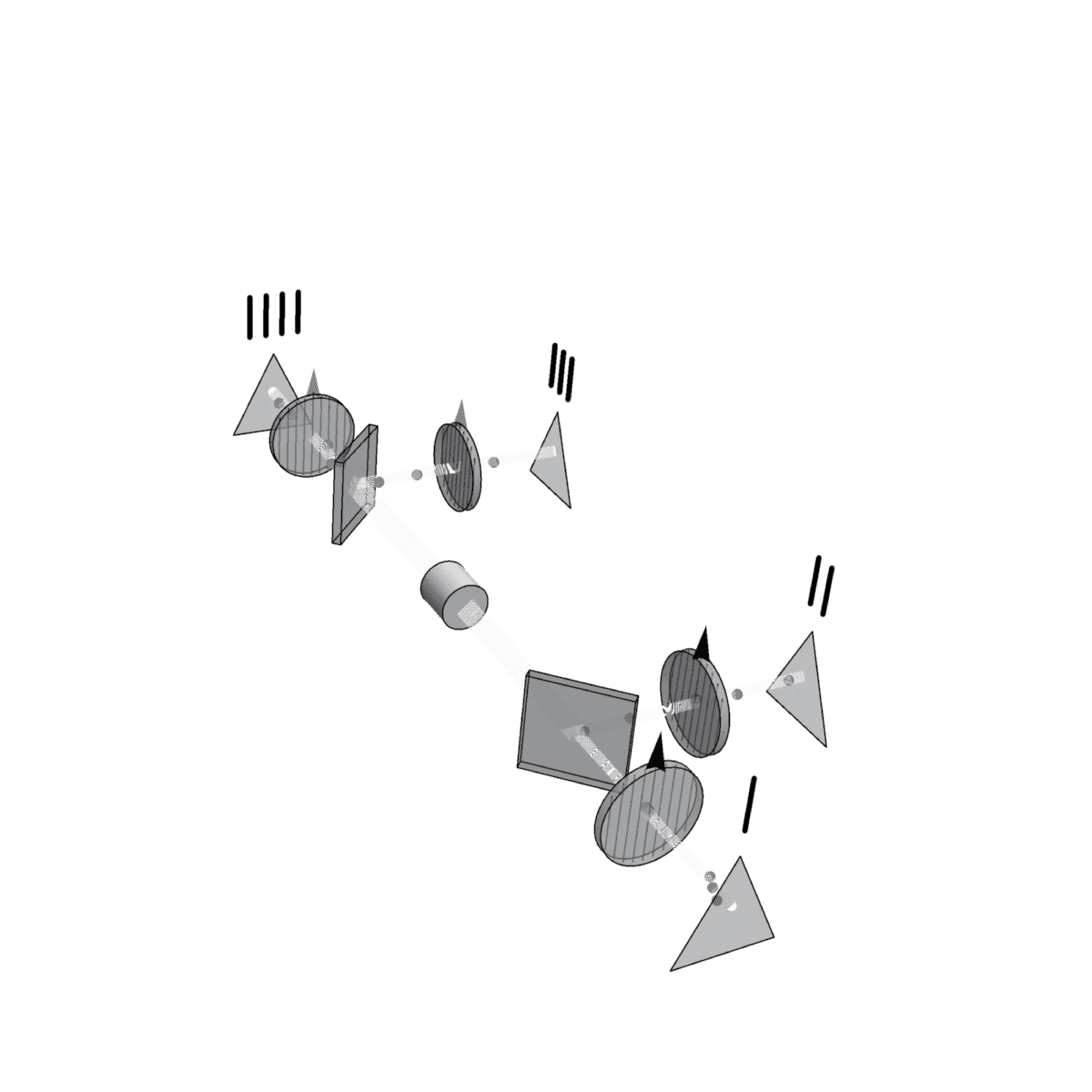
Figure 1: Experimental scheme of the experiment of Alain Aspect: the cylinder in the center is the source of photons, the rectangles are the semitransparent mirrors, the circles are polarizers and the triangles are the detectors

$${{\mathcal{P}}}_{\ddot{Z},\ddot{W}}\left(z_{1},z_{2},z^{{}^{\prime}}_{1},z^{{}^{\prime}}_{2},w_{1},w_{2}\right)=\left\{\begin{array}[]{c}{{\mathcal{P}}}_{W_{1}}(w_{1})\cdot{{\mathcal{P}}}_{W_{2}}(w_{2})\cdot{{\mathcal{P}}}_{Z_{1},Z^{{}^{\prime}}_{1}}(z_{1},z^{{}^{\prime}}_{1},{\vartheta}_{1,1})\Leftarrow(w_{1},w_{2},z_{2},z^{{}^{\prime}}_{2})=(1,1,0,0)\\ {{\mathcal{P}}}_{W_{1}}(w_{1})\cdot{{\mathcal{P}}}_{W_{2}}(w_{2})\cdot{{\mathcal{P}}}_{Z_{1},Z^{{}^{\prime}}_{2}}(z_{1},z^{{}^{\prime}}_{2},{\vartheta}_{1,2})\Leftarrow(w_{1},w_{2},z_{2},z^{{}^{\prime}}_{1})=(1,2,0,0)\\ {{\mathcal{P}}}_{W_{1}}({w}_{1})\cdot{{\mathcal{P}}}_{W_{2}}(w_{2})\cdot{{\mathcal{P}}}_{Z_{2},Z^{{}^{\prime}}_{1}}(z_{2},z^{{}^{\prime}}_{1},{\vartheta}_{2,1})\Leftarrow(w_{1},w_{2},z_{1},z^{{}^{\prime}}_{2})=(2,1,0,0)\\ {{\mathcal{P}}}_{W_{1}}(w_{1})\cdot{{\mathcal{P}}}_{W_{2}}(w_{2})\cdot{{\mathcal{P}}}_{Z_{2},Z^{{}^{\prime}}_{2}}(z_{2},z^{{}^{\prime}}_{2},{\vartheta}_{2,2})\Leftarrow(w_{1},w_{2},z_{1},z^{{}^{\prime}}_{1})=(2,2,0,0)\end{array}\right.,$$ (42)

$$Z_{1}^{{}^{\prime}}:=Z_{3},\quad Z_{2}^{{}^{\prime}}:=Z_{4},\quad\ddot{Z}:=(Z_{1},Z_{2},Z_{1}^{{}^{\prime}},Z_{2}^{{}^{\prime}}),\quad\ddot{W}:=(W_{1},W_{2}),\quad\vartheta_{j,k}:=\theta_{k}^{{}^{\prime}}-\theta_{j},\quad\theta_{1}^{{}^{\prime}}:=\theta_{3},\quad\theta_{2}^{{}^{\prime}}:=\theta_{4}$$

$${\mathcal{P}}_{W_{k}}\left(w_{k}\right)=\left\{\begin{array}[]{ll}p_{k}&\Leftarrow w_{k}=2\\ 1-p_{k}&\Leftarrow w_{k}=1\end{array}\right.,\quad 0\leq p_{k}\leq 1,\quad k\in\left\{1,2\right\}$$

Where $Z_{j}=0$ and $Z_{k}^{{}^{\prime}}=0$ mean the absence of photons, in other words, the path was not correspondent to $(W_{1},W_{2})=(j,k)$ (There is another path).

Therefore, the conditional probability, given that the photons traveled for the route related with the random variables $(W_{1},W_{2})$ with same values, $(w_{1},w_{2})$ will be

$${{\mathcal{P}}}_{\ddot{Z};\ddot{W}}\left(z_{1},z_{2},z^{{}^{\prime}}_{1},z^{{}^{\prime}}_{2};w_{1},w_{2}\right)=$$

$$=\left\{\begin{array}[]{c}{{\mathcal{P}}}_{Z_{1},Z^{{}^{\prime}}_{1}}(z_{1},z^{{}^{\prime}}_{1},{\vartheta}_{1,1})\Leftarrow(w_{1},w_{2},z_{2},z^{{}^{\prime}}_{2})=(1,1,0,0)\\ {{\mathcal{P}}}_{Z_{1},Z^{{}^{\prime}}_{2}}(z_{1},z^{{}^{\prime}}_{2},{\vartheta}_{1,2})\Leftarrow(w_{1},w_{2},z_{2},z^{{}^{\prime}}_{1})=(1,2,0,0)\\ {{\mathcal{P}}}_{Z_{2},Z^{{}^{\prime}}_{1}}(z_{2},z^{{}^{\prime}}_{1},{\vartheta}_{2,1})\Leftarrow(w_{1},w_{2},z_{1},z^{{}^{\prime}}_{2})=(2,1,0,0)\\ {{\mathcal{P}}}_{Z_{2},Z^{{}^{\prime}}_{2}}(z_{2},z^{{}^{\prime}}_{2},{\vartheta}_{2,2})\Leftarrow(w_{1},w_{2},z_{1},z^{{}^{\prime}}_{1})=(2,2,0,0)\end{array}\right.$$ (47)

The conditional expectation (the point sign and comma separates the random variables $(Z,Z^{{}^{\prime}})$ of those observed $(W_{1},W_{2})$) of the product $Z\cdot Z^{{}^{\prime}}$ will be

$${{\mathcal{E}}}_{\ddot{Z};\ddot{W}}(Z_{w_{1}}\cdot Z^{{}^{\prime}}_{w_{2}};w_{1},w_{2})=$$

$$=\sum_{(z_{w_{1}},z_{w_{2}}^{{}^{\prime}})\in\{-1,+1\}^{2}}(z_{w_{1}}\cdot z^{{}^{\prime}}_{w_{2}}\cdot{{\mathcal{P}}}_{Z_{w_{1}},Z_{w_{2}};\ddot{W}}(z_{w_{1}},z_{w_{2}}^{{}^{\prime}};w_{1},w_{2}))$$

therefore

$${{\mathcal{E}}}_{\ddot{Z};\ddot{W}}(Z_{w_{1}}\cdot Z^{{}^{\prime}}_{w_{2}};w_{1},w_{2})=\rm{cos}(2{\vartheta}_{w_{1},w_{2}})$$

thereby, with that understanding, the substitution done in the inequality would not be related to the expected value ${{\mathcal{E}}}_{\ddot{Z}}$, but to the conditional expectation ${{\mathcal{E}}}_{\ddot{Z};\ddot{W}}$, therefore

$$\rm{cos}(2{\vartheta}_{1,1})-\rm{cos}(2{\vartheta}_{1,2})+\rm{cos}(2{\vartheta}_{2,1})+\rm{cos}(2{\vartheta}_{2,2})=$$

$$={{\mathcal{E}}}_{\ddot{Z};\ddot{W}}(Z_{1}\cdot Z^{{}^{\prime}}_{1};1,1)-{{\mathcal{E}}}_{\ddot{Z};\ddot{W}}(Z_{1}\cdot Z^{{}^{\prime}}_{2};1,2)+$$

$$\qquad+{{\mathcal{E}}}_{\ddot{Z};\ddot{W}}(Z_{2}\cdot Z^{{}^{\prime}}_{1};2,1)+{{\mathcal{E}}}_{\ddot{Z};\ddot{W}}(Z_{2}\cdot Z^{{}^{\prime}}_{2};2,2)$$

This result makes no sense from the standpoint of statistic because it is mixing conditional expectation from different events. The conditional probability of a certain event possesses the same properties of the probability theory, but the event that has happened is maintained fixed.

The expectation of $Z_{j}\cdot Z^{{}^{\prime}}_{k}$ with such function of probability would be given by

$${{\mathcal{E}}}_{\ddot{Z},\ddot{W}}\left(Z_{j}\cdot Z^{{}^{\prime}}_{k}\right)={{\mathcal{E}}}_{\ddot{W}}({{\mathcal{E}}}_{\ddot{Z};\ddot{W}}(Z_{j}\cdot Z^{{}^{\prime}}_{k};W_{1},W_{2}))$$

$${{\mathcal{E}}}_{\ddot{Z};\ddot{W}}\left(Z_{j}\cdot Z^{{}^{\prime}}_{k};W_{1},W_{2}\right)=\left\{\begin{array}[]{ll}{{\mathcal{P}}}_{W_{1}}(W_{1})\cdot{{\mathcal{P}}}_{W_{2}}(W_{2})\cdot\mathrm{cos}(2{\vartheta}_{W_{1},W_{2}})&\Leftarrow((j=W_{1})\wedge(k=W_{2}))\\ 0&\Leftarrow\neg((j=W_{1})\wedge(k=W_{2}))\end{array}\right.$$

$${{\mathcal{E}}}_{\ddot{Z},\ddot{W}}\left(Z_{j}\cdot Z^{{}^{\prime}}_{k}\right)={{\mathcal{P}}}_{W_{1}}(j)\cdot{{\mathcal{P}}}_{W_{2}}(k)\cdot\rm{cos}(2{\vartheta}_{j,k})$$

Therefore, the inequality will be

$$|(1-p_{1})\cdot(1-p_{2})\cdot\mathrm{cos}(2{\vartheta}_{1,1})$$

$$\qquad-(1-p_{1})\cdot p_{2}\cdot\mathrm{cos}(2{\vartheta}_{1,2})+$$

$$\qquad+p_{1}\cdot(1-p_{2})\cdot\mathrm{cos}(2{\vartheta}_{2,1})+p_{1}\cdot p_{2}\cdot\mathrm{cos}(2{\vartheta}_{2,2})|\leq$$

$$\leq|(1-p_{1})\cdot(1-p_{2})+(1-p_{1})\cdot p_{2}$$

$$\qquad+p_{1}\cdot(1-p_{2})+p_{1}\cdot p_{2}|=$$

$$=\left|\left(1-p_{1}\right)\cdot\left(1-p_{2}+p_{2}\right)+p_{1}\cdot\left(1-p_{2}+p_{2}\right)\right|$$

$$=\left|\left(1-p_{1}\right)+p_{1}\right|=1\leq 2$$

Hence, besides being reasonable with the theory of the probability, the inequality is mathematically impossible to be violated. Nevertheless, if values are attributed in the original inequality,

$$|\rm{cos}(2{\vartheta}_{1,1})-\rm{cos}(2{\vartheta}_{1,2})+\rm{cos}(2{\vartheta}_{2,1})+\rm{cos}(2{\vartheta}_{2,2})|=$$

$$=|1+1+1+1|=4$$

which shows that it is mathematically possible to violate the original inequality.

IX Computational Simulations

In this section is demonstrated how the sample data is used, evidencing the theoretical comprehention of the previous section, in which is used conditional probability in the calculus of the expected values. So, these theoretical formulas for the set of sample data will be shown in accordance with the theoretical populational formulas.

Computer simulations were conducted, generating up to 100 samples. Each sample was composed of 100 numbers, which estimated the probabilities that are used in the inequality of Clauser-Horne-Shimony-Horne in order to verify if there is a violation or not regarding the samples. The numbers ranged from 1 to 1000; thereby, there was a total of 100 estimates (an estimate of each sample) of probabilities.

The estimations were based on the theory in order to generate samples of a distribution through a sample of uniform distribution. Each number was associated with an event. The events, similar to the Aspect experiment scheme (performed to test the inequality of Clauser-Horne-Shimony-Holt), are as follows:

• When two photons pass through the semitransparent mirrors. The probability of this event is $\frac{1}{4}$. The numbers from 1 to 250 correspond to this event. In this event $j$ is equal to 1

• When the first photon pass through the semitransparent mirrors and the second turns away. The probability of this event is $\frac{1}{4}$. The figures corresponding to this event range from 251 to 500. In this event $j$ is equal to $2$

• When the first photon is deflected and the second photon passes. The probability is $\frac{1}{4}$. The references range from 501 to 750. In this event $j$ is equal to 3

• When two photons fall away. The probability is $\frac{1}{4}$. The correspondent numbers range from 751 to 1000. In the event $j$ is equal to 4.

It is noted that in each of these events the number of intervals associated with them have 250 numbers, so they are equiprobable. To make it simplier, after knowing that the event held at the generated number, n defined as $D$, the value is calculated by the following expression: $D(j-1)\cdot 250$. Thus, it follows that:

• If a number $D$ is generated from 1 to 250, $j$ is 1. Therefore, the following operation is performed: attribute to $D$ the value of $D(j-1)\cdot 250$. So if $j=1$ the value obtained will own $D$, which will be 1 to 250.

• If $j=2$, therefore $251\leq D\leq 500$, the value obtained is $D-250$, which will be 1 and 250

• If $j=3$, therefore $501\leq D\leq 750$, the value obtained is $D-500$, which will be 1 and 250

• If $j=4$, therefore $751\leq D\leq 1000$, the value obtained is $D-750$, which will be 1 and 250

For each of these events, each photon encounters in their paths (any path) a polarizer. Each polarizer is oriented in a particular direction and these orientations are maintained fixed for all 1000 values generated within the sample; changes happen only from sample to sample. By passing through the polarizer, there are two possibilities: either the photon passes or not. Therefore, there are four events for each of the four possible trajectories obtained by passing the mirrors. These four events are:

• Both photons do not pass through the respective polarizers. The event probability is $p_{j}$ (in which $j$ refers to one of four events related to the mirrors). For this event, the new value of $D$ must satisfy the following inequality $0<D\leq p_{j}\cdot 250$

• The first photon does not pass and the second pass. The probability of this event is $(0.5-p_{j})$. For this event, the new value of $D$ must satisfy the following inequality: $p_{j}\cdot 250<D\leq 0.5\cdot 250$

• The first photon passes and the second not. The probability of this event is $(0.5-p_{j})$. For this event, the new value of $D$ must satisfy the following inequality: $0.5<D\leq(1-p_{j})\cdot$ 250

• Both photons pass. The probability of this event is $p_{j}$. For this event, the new value of $D$ must satisfy the following inequality: $(1-p_{j})\cdot 250<D\leq 250$

X Results of simulations

The following tables show the values obtained by the theory as well as the statistics obtained through the simulation.

Each table refers to a set of values that were obtained by fixing the value of parameter ${\theta}_{2}$ (the value of ${\theta}_{2}$ is in the cell of black background, in the upper left corner). At the top (on the cells gray background), are the values of ${\theta}_{3}$ and on left (on gray background of cells) are the values of ${\theta}_{4}$.

The ${\theta}_{1}$ is set to 0 without loss of generality.

The values of ${\theta}_{j}$ (with $j\in\{2,3,4\}$) are submultiples of $\pi$: $\{\frac{\pi}{16},\frac{2\pi}{16},\frac{3\pi}{16},\frac{4\pi}{16},\frac{5\pi}{16},\frac{6\pi}{16},\frac{7\pi}{16}\}$.

There were 7 values for each of the 3 parameters (${\theta}_{2}$ ${\theta}_{3}$ and ${\theta}_{4}$); for example, a total of ${7}^{3}=343$ combinations of values.

The cells are the values and the color bars are related these values. The bars in white represent positive values, and the wider the bars, the higher the values. The gray bars represent negative values and the wider the bars, the smaller the values. Negative values represent a violation of inequalities.

The following will be presented in seven tables (one for each value of ${\theta}_{2}$). They were obtained theoretically from CHSH inequality that is given by:

$$2-|-{{\mathcal{E}}}_{Z_{1},Z_{3}}(Z_{1}\cdot Z_{3})+{{\mathcal{E}}}_{Z_{1},Z_{4}}(Z_{1}\cdot Z_{4})$$

$$+{{\mathcal{E}}}_{Z_{2},Z_{3}}(Z_{2}\cdot Z_{3})+{{\mathcal{E}}}_{Z_{2},Z_{4}}(Z_{2}\cdot Z_{4})|\geq 0$$

performing the following substitution

$${{\mathcal{E}}}_{Z_{j},Z_{k}}(Z_{j}\cdot Z_{k})=\mathrm{cos}(2{\bar{\theta}}_{j,k}),$$ (48)

results in the following inequality

$$2-|-\mathrm{cos}(2{\bar{\theta}}_{1,3})+\mathrm{cos}(2{\bar{\theta}}_{1,4})+\mathrm{cos}(2{\bar{\theta}}_{2,3})+\mathrm{cos}(2{\bar{\theta}}_{2,4})|$$

$$\geq 0$$

and, if the first member of the inequality is greater than or equal to 0, the inequality is obeyed; otherwise there is a violation of inequality.

The values correspond to the value obtained from the first member of inequality (expression that comes before the inequality sign $\geq$).

Table 3: Theoretical values of the first member of the CHSH inequality for ${\theta}_{1}=0$ e ${\theta}_{2}=\frac{\pi}{16}$

In the tables above, it is observed that there were violations (negative values) of the CHSH inequality.

The following tables are obtained through the average of 100 estimates of the CHSH inequality. Each sample contained 1000 elements, which were used to calculate the inequality of CHSH that is given by:

$$\textstyle{\widehat{{\mathcal{E}}}}_{Z_{j},Z_{k}}(Z_{j}\cdot Z_{k})=\frac{n^{--}_{j,k}-{n}^{-+}_{j,k}-n^{+-}_{j,k}+n^{++}_{j,k}}{n_{j,k}}$$ (49)

where

• $n^{--}_{j,k}$ is the number of occurrences of the event when none of the photons passes through the polarizers $j$ and $k$

• $n^{-+}_{j,k}$ is the number of occurrences of the event when the first photon does not pass and the second passes through the polarizers $j$ e $k$, respectively

• $n^{+-}_{j,k}$ is the number of occurrences of the event when the first photon passes and the second not pass the polarizers $j$ e $k$, respectively

• $n^{++}_{j,k}$ is the number of occurrences of the event when both photons pass through the polarizers $j$ e $k$

• $n_{j,k}=(n^{--}_{j,k}+n^{-+}_{j,k}+n^{+-}_{j,k}+n^{++}_{j,k})$ is the number of photons that have taken the path to the polarizers $j$ e $k$ regardless of whether or not it passes through the polarizers.

• $j\in\{1,2\}$ e $k\in\{3,4\}$

The inequality based in each sample is given by

$$2-|-{\widehat{{\mathcal{E}}}}_{Z_{1},Z_{3}}(Z_{1}\cdot Z_{3})+{\widehat{{\mathcal{E}}}}_{Z_{1},Z_{4}}(Z_{1}\cdot Z_{4})$$

$$+{\widehat{{\mathcal{E}}}}_{Z_{2},Z_{3}}(Z_{2}\cdot Z_{3})+{\widehat{{\mathcal{E}}}}_{Z_{2},Z_{4}}(Z_{2}\cdot Z_{4})|\geq 0$$

If the first member of inequality is greater than or equal to 0, the inequality is obeyed; otherwise there is a violation of the inequality. The values correspond to the sample average of 100 values (one value for each of the 100 samples) that were obtained from the first member of the inequality. It was calculated for each sample.

Table 4: Sampled values for ${\theta}_{1}=0$. On the left are the average values of 100 sample values of the first member of CHSH’s inequality. On the right are the standard deviations of the values obtained from 100 samples.

We ought remember that the substitutions (48) and (49) are formulas found in literature. However, according to what was presented in this article, such expected values are expected conditional values.

The formula (49) has its denominador the quantity $n_{j,k}$, that represents only the quantity of observations related to the polarizers $j$ and $k$, evidencing that the estimate of the expected vallue is conditional, that is, it is the estimation when it is considered only the observations in which the particles were taking place specificly for those polarizers $j$ and $k$, disregarding other observations. If such estimation was made for the expected value for the experiment, so we should find in the denominator the quantity $n$ (rather than $n_{j,k}$) because all these observations would be in the calculus of the expected value.

So, in the formula (48), the correct way would be to write

$$\mathcal{E}_{Z_{j},Z_{K}^{{}^{\prime}};\ddot{W}}(Z_{j}\cdot Z_{K}^{{}^{\prime}};j,K)=\cos(2\bar{\theta}_{j,k}),$$

in which (49) would be

$$\hat{\mathcal{E}}_{Z_{j},Z_{k}^{{}^{\prime}};\ddot{W}}(Z_{j}\cdot Z_{k}^{{}^{\prime}};j,K)=\tfrac{n^{--}_{j,k}-{n}^{-+}_{j,k}-n^{+-}_{j,k}+n^{++}_{j,k}}{n_{j,k}}$$

with $k=3$ when $K=1$ and $K=4$ when $K=2$.

As for the CHSH inequality, where the expected values they are estimated from the conditioned probabilities of the event of photons that have or not been deflected to pass through the semitransparent mirrors, the CHSH inequality is kept constant. However, the expected values are as follows:

$${{\mathcal{E}}}_{Z_{j},Z_{k}^{{}^{\prime}}}(Z_{j}\cdot Z_{k}^{{}^{\prime}})={{\mathcal{P}}}_{W_{1},W_{2}}(j,k)\cdot\mathrm{cos}(2{\vartheta}_{j,k})$$

$$Z_{1}^{{}^{\prime}}=Z_{3},\ Z_{2}^{{}^{\prime}}=Z_{4},\ \vartheta_{j,k}=\theta_{j}-\theta_{k}^{{}^{\prime}},\ \theta_{1}^{{}^{\prime}}=\theta_{3},\ \theta_{2}^{{}^{\prime}}=\theta_{4}$$

since ${{\mathcal{P}}}_{W_{1},W_{2}}$ is the function of probability related with the pass or reflection of photons by transparent mirrors, in the case it was adopted that all possible trajectories are equally likely, therefore

$$\textstyle{{\mathcal{P}}}_{W_{1},W_{2}}(j,k)=\frac{1}{4}$$

with $j$ and $k$ belonging to the set $\{1,2,3,4\}$, the expected value that is replaced in the inequality is

$$\textstyle{{\mathcal{E}}}_{Z_{j},Z_{k}}(Z_{j}\cdot Z_{k})=\frac{1}{4}\cdot\rm{cos}(2{\bar{\theta}}_{j,k})$$

resulting in the following inequality

$$\textstyle 2-\left|\frac{-\rm{cos}(2{\bar{\theta}}_{1,3})+\rm{cos}(2{\bar{\theta}}_{1,4})+\rm{cos}(2{\bar{\theta}}_{2,3})+\rm{cos}(2{\bar{\theta}}_{2,4})}{4}\right|\geq 0$$

if the first member of the inequality is greater than or equal to 0, the inequality is obeyed; otherwise there is a violation of the inequality. The values correspond to values that were obtained from the first member of inequality.

Table 5: Theoretical values for ${\theta}_{1}=0$ from first member of the CHSH inequality, modeled via conditional probability

On the tables above, it is observed that there was no violation (negative values) of the CHSH’s inequality (odds conditional modeled).

The following tables show estimates that were obtained by the average of 100 estimates of CHSH’s inequality, which represent the modeled conditional probability. The same samples were previously used, but the calculation of expected values were performed by using the expected sample values (i.e.: the total number of events $n$ were used as the denominator)

$$\textstyle{\widehat{{\mathcal{E}}}}_{Z_{j},Z_{k}}(Z_{j}\cdot Z_{k})=\frac{n^{--}_{j,k}-n^{-+}_{j,k}-n^{+-}_{j,k}+n^{++}_{j,k}}{n}$$

wherein:

• $n^{--}_{j,k}$, $n^{-+}_{j,k}$, $n^{+-}_{j,k}$ e $n^{++}_{j,k}$ have the same previously attributed meaning

• $n=(n_{1,3}+n_{1,4}+n_{2,3}+n_{2,4})$ is the total number of events when there are 1000 occurrences for each sample

Since the CHSH’s inequality can be rewritten as

$$2-|{{\mathcal{E}}}_{Z_{1},Z_{2},Z_{3},Z_{4}}(Z_{1}\cdot Z_{3}+Z_{1}\cdot Z_{4}+Z_{2}\cdot Z_{3}+Z_{2}\cdot Z_{4})|\geq 0$$

then, the inequality (through the sample values) should be calculated by

$$\textstyle 2-\left|\frac{-(n^{--}_{1,3}-n^{-+}_{1,3}-n^{+-}_{1,3}+n^{++}_{1,3})+(n^{--}_{1,4}-n^{-+}_{1,4}-n^{+-}_{1,4}+n^{++}_{1,4})+(n^{--}_{2,3}-n^{-+}_{2,3}-n^{+-}_{2,3}+n^{++}_{2,3})+(n^{--}_{2,4}-n^{-+}_{2,4}-n^{+-}_{2,4}+n^{++}_{2,4})}{n}\right|\geq 0$$

that is

$$\textstyle 2-\left|\frac{-(n^{--}_{1,3}-n^{-+}_{1,3}-n^{+-}_{1,3}+n^{++}_{1,3})+(n^{--}_{1,4}-n^{-+}_{1,4}-n^{+-}_{1,4}+n^{++}_{1,4})+(n^{--}_{2,3}-n^{-+}_{2,3}-n^{+-}_{2,3}+n^{++}_{2,3})+(n^{--}_{2,4}-n^{-+}_{2,4}-n^{+-}_{2,4}+n^{++}_{2,4})}{+(n^{--}_{1,3}+n^{-+}_{1,3}+n^{+-}_{1,3}+n^{++}_{1,3})+(n^{--}_{1,4}+n^{-+}_{1,4}+n^{+-}_{1,4}+n^{++}_{1,4})+(n^{--}_{2,3}+n^{-+}_{2,3}+n^{+-}_{2,3}+n^{++}_{2,3})+(n^{--}_{2,4}+n^{-+}_{2,4}+n^{+-}_{2,4}+n^{++}_{2,4})}\right|\geq 0$$

which is evident that the numerator will always be less or equal to the denominator; thereby, the fraction (as it can be seen) remained between $-1$ and $+$ 1. Therefore, the inequality becomes

$$2-|\pm 1|=2-1=1\geq 0$$

thus, the CHSH’s inequality will never be experimentally violated if the data are modeled by this formula.

Since the expected value is being calculated based on $(Z_{1},Z_{2},Z_{3},Z_{4})$, it makes sense to divide the total number of events related to any of the variables $Z$. Therefore, it is plausible that the denominator is given by $n$.

The inequality based in each sample is given by

$$2-|-{\widehat{{\mathcal{E}}}}_{Z_{1},Z_{3}}(Z_{1}\cdot Z_{3})+{\widehat{{\mathcal{E}}}}_{Z_{1},Z_{4}}(Z_{1}\cdot Z_{4})$$

$$+{\widehat{{\mathcal{E}}}}_{Z_{2},Z_{3}}(Z_{2}\cdot Z_{3})+{\widehat{{\mathcal{E}}}}_{Z_{2},Z_{4}}(Z_{2}\cdot Z_{4})|\geq 0$$

if the first member of the inequality is greater than or equal to 0, the inequality is obeyed; otherwise there is a violation of the inequality. The values correspond to the average sample of the 100 values that were obtained from the calculation of the first member of the inequality for each sample.

Table 6: Sampled values for ${\theta}_{1}=0$. On the left are the average values of 100 sample values of the first member of CHSH’s inequality. On the right are the standard deviations of the values obtained from 100 samples.

XI Analysis and conclusions

In this work, we showed (on the section III) that any dependence between the random variable $Z_{j}$ and the hidden variable $\lambda$ does not change the calculated expected values at all. Therefore any consideration made of the hidden variable $\lambda$ is not relevant to the calculated expected values, this does not mean that such hidden variable can not play any important role in the creation of a model that provides the probability functions used.

In fact, the hidden variable $\lambda$ has its role reduced, essentially because the result of the experiment reduces to only two values ($-1$ and $+1$). In this case, the variable $Z_{j}$ plays the relevant role. Since the CHSH inequality is expressed in terms of expected values of $Z_{j}\cdot Z_{k}$ (this product also results in only two values: $-1$ and $+1$), the focus on the variable $Z_{j}$ compatible with the CHSH inequality, that is, treating $Z_{j}$, instead of $\lambda$, does not influence the conclusions obtained by calculations involving the expected values of $Z_{j}\cdot Z_{k}$.

We presented (on the section V) that the set of probability functions used in the literature can determine a function $\mathcal{P}_{\ddot{Z}}$ in such a way that if we marginalize some of the variables, we retrieve the set of functions used. We also demonstrated (on the section IV), however, that only the CHSH inequality is violated when Kolmogorov’s axioms are violated. Thus, we concluded that although we can find the function that generates the set of functions used, this function does not always respect Kolmogorov’s axioms.

We analyzed the experimental scheme (on the section VIII), and we observed that in the set of functions the probabilities related to the paths taken by the particles are not specified. Through the experimental scheme, we propose to consider the probabilities related to the paths, hence we generated a new set of probabilities, from which, through the conditional probabilities, we could retrieve the set found in the literature. Furthermore we showed that from this new set of probabilities, we can obtain the scaled values of $Z_{j}\cdot Z_{k}$, and that when we substituted in the inequality of CHSH, no violation was found. Therefore, besides this function generate the set of functions of probabilities, it respects the CHSH inequality, which means that it respects the axioms of Komogorov, therefore it is justifiable to say that it is a function of probability and that describes the experiment studied.

We simulated the experiment (on the sections IX and X) to demonstrate how the use of sample data was found in the literature and how the use of the same data would be based on what was presented in this study. These same data that presented the CHSH inequality violation (in the form of use found in the literature), in the new way of using them (which we presented) did not show any violation in the CHSH inequality (whose expected values were calculated based on the Probability functions that contain information on the probability of the particle travel).

In the same formulas of the estimates (used in the literature), we showed (on the section X) that the denominator $n_{j,k}$, demonstrated that the expected value was related to part of the experiment (i.e. related to the path traveled), and that our formula (whose denominator was $n$) besides considering the whole experiment (all observations are considered, same as those related to other paths) it also does not show any violation of the CHSH inequality.

Another result of this work was the proposal (on the section VI) of a basic inequality, from which we can generate the Bell inequality and CHSH inequality. We found that this inequality, when directly used, has no violation. Then we showed that with simple substitutions, we can find Bell inequality and CHSH type inequality, in which violations of the original CHSH inequality would imply in violations of this inequality as well. Thus, we showed the relations between the Bell inequality and the CHSH inequality (in the section VII) and the relationship between the Wigner inequality and the CHSH inequality (on the section IV).

In general, we conclude that the experimental scheme justifies considering that the functions used are in fact conditional probabilities and that, from this consideration, we find new functions of probabilities that give us expected values (with a correction factor) that when we replace in CHSH inequality, no violation occurs, regardless of the parameters.

We conclude that Alain Aspect’s experiment can be modeled by Classical Statistics in order to fully satisfy the CHSH inequality and that CHSH violation would only be possible if there is a violation of Kolmogorov’s axioms.

References

Aspect, Alain and Dalibard, Jean and Roger, Gérard, Experimental Test of Bell’s Inequalities Using Time- Varying Analyzers, Phys. Rev. Lett. 49 (December 1982), no. 25, 1804-1807.

John S. Bell, On the Einstein-Podolsky-Rosen paradox, Physics 1 (1964), 195-200.

Clauser, John F. and Horne, Michael A. and Shimony, Abner and Holt, Richard A., Proposed experiment to test local hidden-variable theories, Phys. Rev. Lett. 23 (October 1969), 880-884

A. Einstein, B. Podolsky, and N. Rosen, Can Quantum-Mechanical Description of Physical Reality Be Considered Complete?, Physical Review 47 (May 1935), no. 10, 777-780.

A. Khrennikov, Epr-bohm experiment and Bell’s inequality: Quantum physics meets probability theory, Theoretical and Mathematical Physics 157 (October 2008), no. 1, 1448-1460.

Andrei Y. Khrennikov, Contextual Approach to Quantum Formalism, 1st ed., Springer, 2009.

M. N. Magalhães, Probabilidade e Variáveis Aleatórias, Edusp, 2006.

Alexsander M. Mood, Franklin A. Graybill, and Duane C. Boes, Introduction to the Theory of Statistics (McGraw-Hill Series in Probability and Statistics), 3rd ed., McGraw-Hill Companies, 1974.

Itamar Pitowsky, Quantum Probability - Quantum Logic, Springer-Verlag Berlin and Heidelberg GmbH & Co. K, 1989.