Graph-based Filtering of Out-of-Vocabulary Words
for Encoder-Decoder Models

Abstract

Encoder-decoder models typically only employ words that are frequently used in the training corpus to reduce the computational costs and exclude noise. However, this vocabulary set may still include words that interfere with learning in encoder-decoder models. This paper proposes a method for selecting more suitable words for learning encoders by utilizing not only frequency but also co-occurrence information, which we capture using the HITS algorithm. We apply our proposed method to two tasks: machine translation and grammatical error correction. For Japanese-to-English translation, this method achieves a BLEU score that is 0.56 points more than that of a baseline. Furthermore, it outperforms the baseline method for English grammatical error correction, with an $\mathrm{F_{0.5}}$-measure that is 1.48 points higher.

1 Introduction

Encoder-decoder models Sutskever et al. (2014) are effective in tasks such as machine translation (Cho et al., 2014; Bahdanau et al., 2015) and grammatical error correction Yuan and Briscoe (2016). Vocabulary in encoder-decoder models is generally selected from the training corpus in descending order of frequency, and low-frequency words are replaced with an unknown word token <unk>. The so-called out-of-vocabulary (OOV) words are replaced with <unk> to not increase the decoder’s complexity and to reduce noise. However, naive frequency-based OOV replacement may lead to loss of information that is necessary for modeling context in the encoder.

This study hypothesizes that vocabulary constructed using unigram frequency includes words that interfere with learning in encoder-decoder models. That is, we presume that vocabulary selection that considers co-occurrence information selects fewer noisy words for learning robust encoders in encoder-decoder models. We apply the hyperlink-induced topic search (HITS) algorithm to extract the co-occurrence relations between words. Intuitively, the removal of words that rarely co-occur with others yields better encoder models than ones that include noisy low-frequency words.

This study examines two tasks, machine translation (MT) and grammatical error correction (GEC) to confirm the effect of decreasing noisy words, with a focus on the vocabulary of the encoder side, because the vocabulary on the decoder side is relatively limited. In a Japanese-to-English MT experiment, our method achieves a BLEU score that is 0.56 points more than that of the frequency-based method. Further, it outperforms the frequency-based method for English GEC, with an $\mathrm{F_{0.5}}$-measure that is 1.48 points higher.

The main contributions of this study are as follows:

1. The simple but effective preprocessing method we propose for vocabulary selection improves encoder-decoder model performance.

2. This study is the first to address noise reduction in the source text of encoder-decoder models.

2 Related Work

There is currently a growing interest in applying neural models to MT (Sutskever et al., 2014; Cho et al., 2014; Bahdanau et al., 2015; Wu et al., 2016) and GEC (Yuan and Briscoe, 2016; Xie et al., 2016; Ji et al., 2017); hence, this study focuses on improving the simple attentional encoder-decoder models that are applied to these tasks.

In the investigation of vocabulary restriction in neural models, Sennrich et al. (2016) applied byte pair encoding to words and created a partial character string set that could express all the words in the training data. They increased the number of words included in the vocabulary to enable the encoder-decoder model to robustly learn contextual information. In contrast, we aim to improve neural models by using vocabulary that is appropriate for a training corpus—not to improve neural models by increasing their vocabulary.

Jean et al. (2015) proposed a method of replacing and copying an unknown word token with a bilingual dictionary in neural MT. They automatically constructed a translation dictionary from a training corpus using a word-alignment model (GIZA++), which finds a corresponding source word for each unknown target word token. They replaced the unknown word token with the corresponding word into which the source word was translated by the bilingual dictionary. Yuan and Briscoe (2016) used a similar method for neural GEC. Because our proposed method is performed as preprocessing, it can be used simultaneously with this replace-and-copy method.

Algorithms that rank words using co-occurrence are employed in many natural language processing tasks. For example, TextRank Mihalcea and Tarau (2004) uses PageRank Brin and Page (1998) for keyword extraction. TextRank constructs a word graph in which nodes represent words, and edges represent co-occurrences between words within a fixed window; TextRank then executes the PageRank algorithm to extract keywords. Although this is an unsupervised method, it achieves nearly the same precision as one state-of-the-art supervised method Hulth (2003). Kiso et al. (2011) used HITS Kleinberg (1999) to select seeds and create a stop list for bootstrapping in natural language processing. They reported significant improvements over a baseline method using unigram frequency. Their graph-based algorithm was effective at extracting the relevance between words, which cannot be grasped with a simple unigram frequency. In this study, we use HITS to retrieve co-occurring words from a training corpus to reduce noise in the source text.

Algorithm 1 HITS

1:hubness vector $i_{0}$

2:adjacency matrix $A$

3:iteration number $\tau$

4:hubness vector $i$

5:authority vector $p$

6:function HITS($i_{0}$, $A$, $\tau$)

7:     $\bm{i}\leftarrow\bm{i_{0}}$

8:     for $t=1,2,...,\tau$ do

9:         $\bm{p}\leftarrow\bm{A^{\mathrm{T}}}\bm{i}$

10:         $\bm{i}\leftarrow\bm{A}\bm{p}$

11:         normalize $i$ and $p$      

12:     return $i$ and $p$

13:end function

3 Graph-based Filtering of OOV Words

3.1 Hubness and authority scores from HITS

HITS, which is a web page ranking algorithm proposed by Kleinberg (1999), computes hubness and authority scores for a web page (node) using the adjacency matrix that represents the web page’s link (edge) transitions. A web page with high authority is linked from a page with high hubness scores, and a web page with a high hubness score links to a page with a high authority score. Algorithm 1 shows pseudocode for the HITS algorithm. Hubness and authority scores converge by setting the iteration number $\tau$ to a sufficiently large value.

3.2 Vocabulary selection using HITS

In this study, we create an adjacency matrix from a training corpus by considering a word as a node and the co-occurrence between words as an edge. Unlike in web pages, co-occurrence between words is nonbinary; therefore, several co-occurrence measures can be used as edge weights. Section 3.3 describes the co-occurrence measures and the context in which co-occurrence is defined.

The HITS algorithm is executed using the adjacency matrix created in the way described above. As a result, it is possible to obtain a score indicating importance of each word while considering contextual information in the training corpus.

Figure 2 shows a word graph example. A word that obtains a high score in the HITS algorithm is considered to co-occur with a variety of words. Figure 2 demonstrates that second order co-occurrence scores (the scores of words co-occurring with words that co-occur with various words Schütze (1998)) are also high.

In this study, words with high hubness scores are considered to co-occur with an important word, and low-scoring words are excluded from the vocabulary. Using this method appears to generate a vocabulary that includes words that are more suitable for representing a context vector for encoder models.

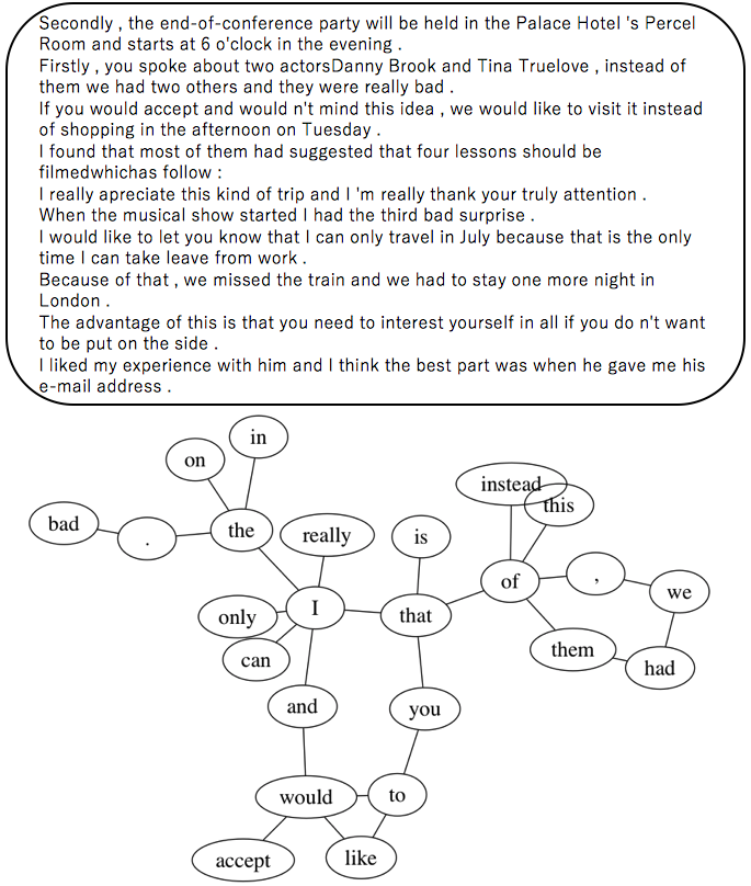
Figure 1: An example word graph created for ten sentences in the training corpus used for GEC.

3.3 Word graph construction

To acquire co-occurrence relations, we use a combination of each word and its peripheral words. Specifically, we combine the target word with surrounding words within window width $N$ and count the occurrences. When defining the context in this way, because the adjacency matrix becomes symmetric, the same hubness and authority scores can be obtained. Figure 2 shows an example of co-occurrence in which $N$ is set to two.

We use raw co-occurrence frequency (Freq) and positive pointwise mutual information (PPMI) between words as the ($x,y$) element $A_{xy}$ of the adjacency matrix. However, naive PPMI reacts sensitively to low-frequency words in a training corpus. To account for high-frequency, we weight the PMI by the logarithm of the number of co-occurrences and use PPMI based on this weighted PMI (Equation 2).

$$A_{xy}^{freq}=|x,y|$$ (1)

$$A_{xy}^{ppmi}=\mathrm{max}(0,\mathrm{pmi}(x,y)+\log_{2}|x,y|)$$ (2)

Equation 3 is the PMI of target word $x$ and co-occurrence word $y$. $M$ is the number of tokens of the combination, $|x,*|$ and $|*,y|$ are the number of token combinations when fixing target word $x$ and co-occurrence word $y$, respectively.

$$\mathrm{pmi}(x,y)=\log_{2}\frac{M\cdot|x,y|}{|x,*||*,y|}$$ (3)

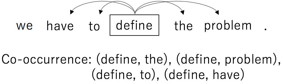
Figure 2: An example of co-occurrence context.

4 Machine Translation

4.1 Experimental setting

In the first experiment, we conduct a Japanese-to-English translation using the Asian Scientific Paper Excerpt Corpus (ASPEC; Nakazawa et al., 2016). We follow the official split of the train, development, and test sets. As training data, we use only the first 1.5 million sentences sorted by sentence alignment confidence to obtain a Japanese–English parallel corpus (sentences of more than 60 words are excluded). Our training set consists of 1,456,278 sentences, development set consists of 1,790 sentences, and test set consists of 1,812 sentences. The training set has 247,281 Japanese word types and 476,608 English word types.

The co-occurrence window width $N$ is set to two. For combinations that co-occurred only once within the training corpus, we set the value of element $A_{xy}$ of the adjacency matrix to zero. The iteration number $\tau$ of the HITS algorithm is set to 300. As mentioned in Section 1, we only use the proposed method on the encoder side.

For this study’s neural MT model, we implement global dot attention Luong et al. (2015). We train a baseline model that uses vocabulary that is determined by its frequency in the training corpus. Vocabulary size is set to 100K on the encoder side and 50K on the decoder side. Additionally, we conduct an experiment of varying vocabulary size of the encoder to 50K in the baseline and PPMI to investigate the effect of vocabulary size. Unless otherwise noted, we conduct an analysis of the model using the vocabulary size of 100K. The number of dimensions for each of the hidden and embedding layers is 512. The mini-batch size is 150. AdaGrad is used as an optimization method with an initial learning rate of 0.01. Dropout is applied with a probability of 0.2.

For this experiment, a bilingual dictionary is prepared for postprocessing unknown words Jean et al. (2015). When the model outputs an unknown word token, the word with the highest attention score is used as a query to replace the unknown token with the corresponding word from the dictionary. If not in the dictionary, we replace the unknown word token with the source word (unk_rep). This dictionary is created based on word alignment obtained using fast_align Dyer et al. (2013) on the training corpus.

We evaluate translation results using BLEU scores Papineni et al. (2002).

	baseline	HITS (Freq)	HITS (PPMI)
BLEU (50K)	22.24	-	22.40
BLEU (100K)	22.21	22.25	22.77
$p$-value	-	0.35	0.01

Table 1: BLEU scores for Japanese-to-English translation. The parentheses indicate vocabulary size of the encoder.

	COMMON outputs		DIFF outputs
	baseline	PPMI	baseline	PPMI
BLEU	22.33	22.98	21.44	21.98

Table 2: BLEU scores of the COMMON and DIFF outputs.

4.2 Results

Table 4 shows the translation accuracy (BLEU scores) and $p$-value of a significance test ($p<0.05$) by bootstrap resampling Koehn (2004). The PPMI model improves translation accuracy by 0.56 points in Japanese-to-English translation, which is a significant improvement.

Next, we examine differences in vocabulary by comparing each model with the baseline. Compared to the vocabulary of the baseline in 100K setting, Freq and PPMI replace 16,107 and 17,166 types, respectively; compared to the vocabulary of the baseline in 50K setting, PPMI replaces 4,791 types.

src	有用 物質 の 分離 ・ 抽出 , 反応 性 向上 , 新 材料 創製 , 廃棄 物 処理 , 分析 等 の 分野 が ある 。
baseline	there are fields such as separation , extraction , extraction , improvement of new material creation , waste treatment , analysis , etc .
Freq	there are separation and extraction of useful substances , the improvement of reactivity , new material creation , waste treatment and analysis .
PPMI	there are the fields such as separation and extraction of useful materials , the reaction improvement , new material creation , waste treatment , analysis , etc …
ref	the application fields are separation and extraction of useful substances , reactivity improvement , creation of new products , waste treatment , and chemical analysis .

Table 3: An example of Japanese-to-English translation on a source sentence from COMMON.

4.3 Analysis

According to Table 4, the performance of Freq is almost the same as that of the baseline. When examining the differences in selected words in vocabulary between PPMI and Freq, we find that PPMI selects more low-frequency words in the training corpus compared to Freq, because PPMI deals with not only frequency but also co-occurrence.

The effect of unk_rep is almost the same in the baseline as in the proposed method, which indicates that the proposed method can be combined with other schemes as a preprocessing step.

As a comparison of the vocabulary size 50K and 100K, the BLEU score of 100K is higher than that of 50K in PPMI. Moreover, the BLEU scores are almost the same in the baseline. We suppose that the larger the vocabulary size of encoder, the more noisy words the baseline includes, while the PPMI filters these words. That is why the proposed method works well in the case where the vocabulary size is large.

To examine the effect of changing the vocabulary on the source side, the test set is divided into two subsets: COMMON and DIFF. The former (1,484 sentences) consists of only the common vocabulary between the baseline and PPMI, whereas the latter (328 sentences) includes at least one word excluded from the common vocabulary.

Table 2 shows the translation accuracy of the COMMON and DIFF outputs. Translation performance of both corpora is improved.

In order to observe how PPMI improves COMMON outputs, we measure the similarity of the baseline and PPMI output sentences by counting the exact same sentences. In the COMMON outputs, 72 sentence pairs (4.85%) are the same, whereas 9 sentence pairs are the same in the DIFF outputs (2.74%). Surprisingly, even though it uses the same vocabulary, PPMI often outputs different but fluent sentences.

Table 3 shows an example of Japanese-to-English translation. The outputs of the proposed method (especially PPMI) are improved, despite the source sentence being expressed with common vocabulary; this is because the proposed method yielded a better encoder model than the baseline.

5 Grammatical Error Correction

5.1 Experimental setting

The second experiment addresses GEC. We combine the FCE public dataset Yannakoudakis et al. (2011), NUCLE corpus Dahlmeier et al. (2013), and English learner corpus from the Lang-8 learner corpus Mizumoto et al. (2011) and remove sentences longer than 100 words to create a training corpus. From the Lang-8 learner corpus, we use only the pairs of erroneous and corrected sentences. We use 1,452,584 sentences as a training set (502,908 types on the encoder side and 639,574 types on the decoder side). We evaluate the models’ performances on the standard sets from the CoNLL-14 shared task Ng et al. (2014) using CoNLL-13 data as a development set (1,381 sentences) and CoNLL-14 data as a test set (1,312 sentences). We employ $\mathrm{F_{0.5}}$ as an evaluation measure for the CoNLL-14 shared task.

	baseline		PPMI
	50K	150K	50K	150K
Precision	48.09	46.53	49.45	49.23
Recall	8.30	8.50	8.61	9.02
$\mathrm{F_{0.5}}$	24.55	24.55	25.37	26.03

Table 4: $\mathrm{F_{0.5}}$ results on the CoNLL-14 test set.

	COMMON outputs		DIFF outputs
	baseline	PPMI	baseline	PPMI
P	48.26	60.07	9.40	17.32
R	0.01	0.01	0.01	0.02
$\mathrm{F_{0.5}}$	0.04	0.04	0.04	0.08

Table 5: $\mathrm{F_{0.5}}$ of COMMON and DIFF outputs.

We use the same model as in Section 4.1 as a neural model for GEC. The models’ parameter settings are similar to the MT experiment, except for the vocabulary and batch sizes. In this experiment, we set the vocabulary size on the encoder and decoder sides to 150K and 50K, respectively. Additionally, we conduct the experiment of changing vocabulary size of the encoder to 50K to investigate the effect of the vocabulary size. Unless otherwise noted, we conduct an analysis of the model using the vocabulary size of 150K. The mini-batch size is 100.

5.2 Result

Table 5 shows the performance of the baseline and proposed method. The PPMI model improves precision and recall; it achieves a $\mathrm{F_{0.5}}$-measure 1.48 points higher than the baseline method.

In setting the vocabulary size of encoder to 150K, PPMI replaces 37,185 types from the baseline; in the 50K setting, PPMI replaces 10,203 types.

src	Genetic refers the chance of inheriting a disorder or disease .
baseline	Genetic refers the chance of inheriting a disorder or disease .
PPMI	Genetic refers to the chance of inheriting a disorder or disease .
gold	Genetic risk refers to the chance of inheriting a disorder or disease .

Table 6: An example of GEC using a source sentence from COMMON.

5.3 Analysis

The $\mathrm{F_{0.5}}$ of the baseline is almost the same while the PPMI model improves the score in the case where the vocabulary size increases. Similar to MT, we suppose that the PPMI filters noisy words.

As in Section 4.3, we perform a follow-up experiment using two data subsets: COMMON and DIFF, which contain 1,072 and 240 sentences, respectively.

Table 5 shows the accuracy of the error correction of the COMMON and DIFF outputs. Precision increases by 11.81 points, whereas recall remains the same for the COMMON outputs.

In GEC, approximately 20% of COMMON’s output pairs differ, which is caused by the differences in the training environment. Unlike MT, we can copy OOV in the target sentence from the source sentence without loss of fluency; therefore, our model has little effect on recall, whereas its precision improves because of noise reduction.

Table 6 shows an example of GEC. The proposed method’s output improves when the source sentence is expressed using common vocabulary.

6 Discussion

We described that the proposed method has a positive effect on learning the encoder. However, we have a question; what affects the performance? We conduct an analysis of this question in this section.

First, we count the occurrence of the words included only in the baseline or PPMI in the training corpus. We also show the number of the tokens per types (“Ave. tokens”) included only in either the baseline or PPMI vocabulary.

	MT		GEC
	baseline	PPMI	baseline	PPMI
tokens	52,700	27,364	126,884	70,003
Ave. tokens	3.07	1.59	3.36	1.85

Table 7: Number of words included only in either the baseline or PPMI vocabulary.

The result is shown in Table 7. We find that the proposed method uses low-frequency words instead of high-frequency words in the training corpus. This result suggests that the proposed method works well despite the fact that the encoder of the proposed method encounters more <unk> than the baseline. This is because the proposed method excludes words that may interfere with the learning of encoder-decoder models.

Second, we conduct an analysis of the POS of the words in GEC to find why increasing OOV improves the learning of encoder-decoder models. Specifically, we apply POS tagging to the training corpus and calculate the occurrence of the POS of the words only included in the baseline or PPMI. We use NLTK as a POS tagger.

Table 8 shows the result. It is observed that NOUN is the most affected POS by the proposed method and becomes often represented by <unk>. NOUN words in the vocabulary of the baseline contain some non-English words, such as Japanese or Korean. These words should be treated as OOV but the baseline fails to exclude them using only the frequency. According to Table 8, NUM is also affected by the proposed method. NUM words of the baseline include a simple numeral such as “119”, in addition to incorrectly segmented numerals such as “514&objID”. This word appears 25 times in the training corpus owing to the noisy nature of Lang-8. We suppose that the proposed method excludes these noisy words and has a positive effect on training.

POS	baseline	PPMI	ALL
NOUN	92,693	44,472	4,644,478
VERB	11,066	10,099	3,597,895
PRON	127	107	1,869,422
ADP	626	685	1,836,193
DET	128	202	1,473,391
ADJ	13,855	12,270	1,429,056
ADV	2,032	1,688	931,763
PRT	319	75	615,817
CONJ	62	28	537,346
PUNCT	110	11	223,573
NUM	5,585	299	207,487
OTHER	281	67	5,209
Total	126,884	70,003	17,371,630

Table 8: Number of the POS of words only included in the baseline or PPMI.

7 Conclusion

In this paper, we proposed an OOV filtering method, which considers word co-occurrence information for encoder-decoder models. Unlike conventional OOV handling, this graph-based method selects the words that are more suitable for learning encoder models by considering contextual information. This method is effective for not only machine translation but also grammatical error correction.

This study employed a symmetric matrix (similar to skip-gram with negative sampling) to express relationships between words. In future research, we will develop this method by using vocabulary obtained by designing an asymmetric matrix to incorporate syntactic relations.

References

- Bahdanau et al. (2015) Dzmitry Bahdanau, Kyunghyun Cho, and Yoshua Bengio. 2015. Neural machine translation by jointly learning to align and translate. In Proc. of ICLR.
- Brin and Page (1998) Sergey Brin and Lawrence Page. 1998. The anatomy of a large-scale hypertextual web search engine. Comput. Netw. ISDN Syst. 30(1-7):107–117. https://doi.org/10.1016/S0169-7552(98)00110-X.
- Cho et al. (2014) Kyunghyun Cho, Bart van Merrienboer, Caglar Gulcehre, Dzmitry Bahdanau, Fethi Bougares, Holger Schwenk, and Yoshua Bengio. 2014. Learning phrase representations using RNN encoder–decoder for statistical machine translation. In Proc. of EMNLP. pages 1724–1734. http://www.aclweb.org/anthology/D14-1179.
- Dahlmeier et al. (2013) Daniel Dahlmeier, Hwee Tou Ng, and Siew Mei Wu. 2013. Building a large annotated corpus of learner English: The NUS corpus of learner English. In Proc. of BEA. pages 22–31. http://www.aclweb.org/anthology/W13-1703.
- Dyer et al. (2013) Chris Dyer, Victor Chahuneau, and Noah A. Smith. 2013. A simple, fast, and effective reparameterization of IBM model 2. In Proc. of NAACL-HLT. pages 644–648. http://www.aclweb.org/anthology/N13-1073.
- Hulth (2003) Anette Hulth. 2003. Improved automatic keyword extraction given more linguistic knowledge. In Proc. of EMNLP. pages 216–223. http://www.aclweb.org/anthology/W03-1028.
- Jean et al. (2015) Sébastien Jean, Orhan Firat, Kyunghyun Cho, Roland Memisevic, and Yoshua Bengio. 2015. Montreal neural machine translation systems for WMT15. In Proc. of WMT. pages 134–140. http://aclweb.org/anthology/W15-3014.
- Ji et al. (2017) Jianshu Ji, Qinlong Wang, Kristina Toutanova, Yongen Gong, Steven Truong, and Jianfeng Gao. 2017. A nested attention neural hybrid model for grammatical error correction. In Proc. of ACL. pages 753–762. http://aclweb.org/anthology/P17-1070.
- Kiso et al. (2011) Tetsuo Kiso, Masashi Shimbo, Mamoru Komachi, and Yuji Matsumoto. 2011. HITS-based seed selection and stop list construction for bootstrapping. In Proc. of ACL. pages 30–36. http://www.aclweb.org/anthology/P11-2006.
- Kleinberg (1999) Jon M. Kleinberg. 1999. Authoritative sources in a hyperlinked environment. J. ACM 46(5):604–632. https://doi.org/10.1145/324133.324140.
- Koehn (2004) Philipp Koehn. 2004. Statistical significance tests for machine translation evaluation. In Proc. of EMNLP. pages 388–395. http://www.aclweb.org/anthology/W04-3250.
- Luong et al. (2015) Thang Luong, Hieu Pham, and Christopher D. Manning. 2015. Effective approaches to attention-based neural machine translation. In Proc. of EMNLP. pages 1412–1421. http://aclweb.org/anthology/D15-1166.
- Mihalcea and Tarau (2004) Rada Mihalcea and Paul Tarau. 2004. TextRank: Bringing order into texts. In Proc. of EMNLP. pages 404–411. http://www.aclweb.org/anthology/W04-3252.
- Mizumoto et al. (2011) Tomoya Mizumoto, Mamoru Komachi, Masaaki Nagata, and Yuji Matsumoto. 2011. Mining revision log of language learning sns for automated Japanese error correction of second language learners. In Proc. of IJCNLP. pages 147–155. http://www.aclweb.org/anthology/I11-1017.
- Nakazawa et al. (2016) Toshiaki Nakazawa, Manabu Yaguchi, Kiyotaka Uchimoto, Masao Utiyama, Eiichiro Sumita, Sadao Kurohashi, and Hitoshi Isahara. 2016. ASPEC: Asian scientific paper excerpt corpus. In Proc. of LREC. pages 2204–2208.
- Ng et al. (2014) Hwee Tou Ng, Siew Mei Wu, Ted Briscoe, Christian Hadiwinoto, Raymond Hendy Susanto, and Christopher Bryant. 2014. The CoNLL-2014 shared task on grammatical error correction. In Proc. of CoNLL Shared Task. pages 1–14.
- Papineni et al. (2002) Kishore Papineni, Salim Roukos, Todd Ward, and Wei-Jing Zhu. 2002. BLEU: a method for automatic evaluation of machine translation. In Proc. of ACL. pages 311–318. http://www.aclweb.org/anthology/P02-1040.
- Schütze (1998) Hinrich Schütze. 1998. Automatic word sense discrimination. Computational Linguistics 24(1):97–123. http://dl.acm.org/citation.cfm?id=972719.972724.
- Sennrich et al. (2016) Rico Sennrich, Barry Haddow, and Alexandra Birch. 2016. Neural machine translation of rare words with subword units. In Proc. of ACL. pages 1715–1725. http://www.aclweb.org/anthology/P16-1162.
- Sutskever et al. (2014) Ilya Sutskever, Oriol Vinyals, and Quoc V Le. 2014. Sequence to sequence learning with neural networks. In Proc. of NIPS. pages 3104–3112.
- Wu et al. (2016) Yonghui Wu, Mike Schuster, Zhifeng Chen, Quoc V Le, Mohammad Norouzi, Wolfgang Macherey, Maxim Krikun, Yuan Cao, Qin Gao, Klaus Macherey, et al. 2016. Google’s neural machine translation system: Bridging the gap between human and machine translation. arXiv preprint arXiv:1609.08144 .
- Xie et al. (2016) Ziang Xie, Anand Avati, Naveen Arivazhagan, Dan Jurafsky, and Andrew Y Ng. 2016. Neural language correction with character-based attention. arXiv preprint arXiv:1603.09727 .
- Yannakoudakis et al. (2011) Helen Yannakoudakis, Ted Briscoe, and Ben Medlock. 2011. A new dataset and method for automatically grading ESOL texts. In Proc. of ACL-HLT. pages 180–189. http://www.aclweb.org/anthology/P11-1019.
- Yuan and Briscoe (2016) Zheng Yuan and Ted Briscoe. 2016. Grammatical error correction using neural machine translation. In Proc. of NAACL-HLT. pages 380–386. http://www.aclweb.org/anthology/N16-1042.