On mass conservation for ice sheets

Abstract

A new continuum-mechanical formulation is proposed which encompasses all material processes within and surrounding an ice sheet. Using this formulation, the balance of mass and free-surface relations for ice sheets are derived and elaborated upon. The resulting three-dimensional mass-balance relation is then integrated vertically to produce an ice-sheet quasi-mass-balance relation in the horizontal plane, and is demonstrated to reduce velocity errors in regions with high magnitude surface gradients. An analytic velocity satisfying the corrected mass-balance relation is formulated as a means to verify future numerical ice-sheet models.

In memory of Professor Toma ‘Thomas’ Tonev, 1945–2015.

35L51, 35Q86, 76A05, 76T30, 35L65,

00.0000/000000000

Notation.

$u$	rank-zero tensor (scalar)
$\underline{u}$	rank-one tensor (vector)
$\underline{\underline{u}}$	rank-two tensor (matrix)
$\underline{u}^{\intercal},\underline{\underline{u}}^{\intercal}$	transpose of tensor $\underline{u}$ or $\underline{\underline{u}}$
$\underline{u}_{\perp}$, $\underline{u}_{\|}$	perp./tangent comp. of $\underline{u}$
$\underline{u}\cdot\underline{v}$	scalar product
$\bar{u},\bar{\underline{u}}$	vertical average of $u$ or $\underline{u}$
$\hat{\underline{u}}$	normal vector $\hat{\underline{u}}=\underline{u}/\|\underline{u}\|$
$\partial_{i}u$	partial deriv. of $u$ w.r.t. $i$
$\mathrm{d}_{i}u$	derivative of $u$ w.r.t. $i$
$\nabla u$	gradient of $u$
$\nabla\cdot\underline{u}$	divergence of $\underline{u}$
$\dot{u}$	time derivative of $u$
$\mathring{u}$	non-diff. rate of change of $u$

Empiricals.

$\rho_{\mathrm{a}}$	$\sim 1.2$	kg m-3	air density
$\rho_{\mathrm{i}}$	$\sim 910$	kg m-3	ice density
$\rho_{\mathrm{w}}$	$\sim 1000$	kg m-3	water density
$\rho_{\mathrm{sw}}$	$\sim 1028$	kg m-3	seawater den.

Superscripts.

$+$	exterior region
$-$	interior region
$\mathrm{e}$	sub-element region

Subscripts.

$x,y,z$	Cartesian coordinate
$\mathrm{s}$	solid
$\mathrm{\ell}$	liquid
$\mathrm{v}$	vapor
$\mathrm{i}$	ice
$\mathrm{w}$	water
$\mathrm{sw}$	seawater
$\mathrm{a}$	air
$\mathrm{B}$	lower surface
$\mathrm{S}$	upper surface

Variables.

$\omega$	–	mass fraction
$\alpha$	–	volume fraction
$m$	kg	mass
$\rho$	kg m-3	mass density
$F$	m	implicit surface
$x$	m	position
$u$	m s-1	fluid velocity
$w$	m s-1	surface velocity
$q$	kg m-2	surface-mass density
$\sigma$	Pa	stress
$\varOmega$	m3	interior domain
$\varGamma$	m2	boundary of $\varOmega$
$\varSigma$	m2	discontinuity surface

Introduction

Continuum-mechanical formulations which describe the dynamics of ice sheets and glaciers are complicated due to varied environmental interactions, including the atmosphere, lithosphere, sub- and supra-surface lakes, the oceans, etc; clearly-defined discontinuities within the ice-sheet interior; water transport within and surrounding the ice sheet; and conservation laws associated with compressible multi-phase flows. In order to describe these processes, the basis of a new continuum-mechanical formulation for ice sheets—i. e. mass conservation—is herein proposed.

It has been taken axiomatic within the glaciological community that the evolution of ice-sheet mass is governed by the equation $\partial_{t}H+\nabla\cdot\left(H\underline{\bar{u}}\right)=\mathring{S}+\mathring{B}$, with ice thickness $H$, vertically-averaged ice velocity $\underline{\bar{u}}$, and accumulation/ablation functions over upper and lower surfaces $\mathring{S}$ and $\mathring{B}$. This equation is commonly stated without derivation, justification, or citations; e. g., equations (28) of [15], (1) of [35], (1) of [5], (6) of [29], (2) of [32], (2.13) of [18], and (1) of [22]. The original use of this relation is unknown; however, one may conjecture that this relation has been formed by assuming that the ice-sheet thickness flux in the $xy$ plane can be described with a forcing term $\mathring{H}=\mathring{S}+\mathring{B}$ that is independent of variations in the upper surface $S$ and lower surface $B$. The results of [12] are herein revisited and lead to the conclusion that this assumption is inappropriate over regions associated with steep surface gradients. The correct vertically-integrated mass-balance equation for incompressible materials such as ice is thereafter derived and elaborated upon.

The basis of any numerical model consists of an analytic solution; that is, the verification of computer-code integrity is necessary for numerical model development. Therefore, in order for new numerical models of ice-sheet dynamics to make use of the concepts developed here, an analytic velocity is proposed which satisfies any combination of upper- and lower-surface mass-balance boundary conditions.

The paper is organized as follows. A description of the cryosphere environment and associated interactions is first presented in Section 1, followed by a description of the surface-mass balance in Section 2, an explanation of global- and local-mass conservation in Section 3, derivation of the kinematic free-surface relations in Section 4, derivation of the vertically-integrated mass-balance equation and error quantification associated with commonly-applied assumptions in Section 5, and formulation of a generalized three-dimensional analytic solution for incompressible mass conservation incorporating both the upper and lower surface-mass-balance terms in Section 6. The paper is concluded with a short statement of intended future work in Section 7.

1 The multi-phase cryosphere

Ice sheets and glaciers may be represented as a system of differential multi-phase equations of disperse flow (cf. [4]). These equations were first stated for binary ice and water mixtures by [12], which is a modification to concepts developed in [8]. The formulation developed here incorporates statements of vapor conservation, which is required to describe surface processes such as evaporation, condensation, sublimation, and deposition (cf. [3]). Within the ice interior, vapor conservation is needed to describe mechanical effects such as firn densification or closure of cavities between ice grains.

Figure 1: Two-material domain with interior volume $\varOmega^{-}$ and exterior volume $\varOmega^{+}$ which share a common boundary $\varSigma$. The exterior surface $\partial\varOmega=\varGamma$ is in this case given by $\varGamma=\varGamma^{+}/\left(\varGamma^{+}\cap\varGamma^{-}\right)$; this analysis does not consider effects over $\varGamma$.

Consider the cryosphere domain $\varOmega=\varOmega(\underline{x},t)$ composed of the ice-sheet interior $(-)$ and exterior $(+)$ domains $\varOmega^{\pm}=\varOmega^{\pm}(\underline{x},t)$ such that $\varOmega=\varOmega^{-}\cup\varOmega^{+}$ and $\varOmega^{-}\cap\varOmega^{+}=\emptyset$. Further define the boundaries $\varGamma^{\pm}=\partial\varOmega^{\pm}(\underline{x},t)$, ice-sheet surface $\varSigma=\varGamma^{-}\cap\varGamma^{+}$, and outward-pointing-unit normals $\underline{\hat{n}}^{\pm}$ (Fig. 1). Imagine within $\varOmega$ an ice-mixture mass density $\rho=\rho(\underline{x},t)$ which is composed of some amount of solid ($\mathrm{s}$), liquid ($\mathrm{\ell}$), and vapor ($\mathrm{v}$) components, each moving relative to barycentric velocity $\underline{u}=\underline{u}(\underline{x},t)$ defined by [21] satisfying

(1) $$\rho^{\pm}\underline{u}^{\pm}=\rho_{\mathrm{s}}^{\pm}\underline{u}_{\mathrm{s}}^{\pm}+\rho_{\mathrm{\ell}}^{\pm}\underline{u}_{\mathrm{\ell}}^{\pm}+\rho_{\mathrm{v}}^{\pm}\underline{u}_{\mathrm{v}}^{\pm},\hskip 42.67912pt\rho^{\pm}=\rho_{\mathrm{s}}^{\pm}+\rho_{\mathrm{\ell}}^{\pm}+\rho_{\mathrm{v}}^{\pm},$$

where the extrinsic-mass densities $\rho_{k}=\rho_{k}(\underline{x},t)$, $k=\mathrm{s},\mathrm{\ell},\mathrm{v}$ are defined as the component masses per unitary volume, and are connected bijectively to the constant empirically-derived ice ($\mathrm{i}$), water ($\mathrm{w}$), and air ($\mathrm{a}$) intrinsic-mass densities $\rho_{q}$ for $q=\mathrm{i},\mathrm{w},\mathrm{a}$ via

(2) $$\rho_{\mathrm{s}}^{\pm}=\alpha_{\mathrm{s}}^{\pm}\rho_{\mathrm{i}},\hskip 28.45274pt\rho_{\mathrm{\ell}}^{\pm}=\alpha_{\mathrm{\ell}}^{\pm}\rho_{\mathrm{w}},\hskip 28.45274pt\rho_{\mathrm{v}}^{\pm}=\alpha_{\mathrm{v}}^{\pm}\rho_{\mathrm{a}},$$

where $\alpha_{k}^{\pm}=\alpha_{k}^{\pm}(\underline{x},t)$ is the volume fraction of phase $k$ with property $\sum_{k}\alpha_{k}^{\pm}=1$.

Remark 1.1.

Stating the extrinsic-mass density of each phase in the manner of Eqs. 1 and 2 allows the mass to vary continuously both within and surrounding the ice sheet domain $\varOmega^{-}$. For example, the atmosphere boundary will have $\rho_{\mathrm{\ell}}^{+}=\rho_{\mathrm{w}}$ in regions in contact with collected surface water, the basal surface may have a range of values $\rho_{\mathrm{\ell}}^{+}\in[0,\rho_{\mathrm{w}}]$ depending on the saturation of the sub-glacial aquifer, and $\rho_{\mathrm{\ell}}^{+}=\rho_{\mathrm{sw}}$ over regions in contact with the ocean.

Division of Eq. 1₂ by $\rho^{\pm}$ produces the equation of state

(3) $$1=\omega_{\mathrm{s}}^{\pm}+\omega_{\mathrm{\ell}}^{\pm}+\omega_{\mathrm{v}}^{\pm},\hskip 42.67912pt\omega_{k}^{\pm}=\rho_{k}^{\pm}/\rho^{\pm},\hskip 14.22636ptk=\mathrm{s},\mathrm{\ell},\mathrm{v};$$

where $\omega_{k}^{\pm}=\omega_{k}^{\pm}(\underline{x},t)$ is the mass fraction of phase $k$. In addition, taking the derivative of mixture density Eq. 1₂ with respect to time yields

(4) $$\mathring{\rho}=\mathring{\rho}_{\mathrm{s}}^{\pm}+\mathring{\rho}_{\mathrm{\ell}}^{\pm}+\mathring{\rho}_{\mathrm{v}}^{\pm} \text{in }\varOmega$$

with individual components $\mathring{\rho}_{k}$ in units of mass per unitary volume per time, and are clearly positive for mass gain and negative for mass loss.

In addition to mass fluctuations within $\varOmega$ given by Eq. 4, there will be also be mass-phase changes on the surface $\varSigma$ due to interactions between the $(\pm)$ domains given by

(5) $$\mathring{q}=\mathring{q}_{\mathrm{s}}+\mathring{q}_{\mathrm{\ell}}+\mathring{q}_{\mathrm{v}} \text{on }\varSigma$$

where $\mathring{q}_{k}$ are in units of mass per unitary surface area per time, and are positive for mass gain and negative for mass loss over the surface $\varSigma$. The following proposition illustrates that source terms Eqs. 4 and 5 are in fact homogeneous:

Proposition 1.2.

The total rate of change of the mass density $\rho=\rho(\underline{x},t)$ and surface-mass density $q=q(\underline{x},t)$ given by Eq. 4 and Eq. 5 are respectively $\mathring{\rho}=0$ and $\mathring{q}=0$ for all $\underline{x}$ and $t$.

Proof 1.3.

Considering all mass sources and sinks of partial densities Eq. 2, the total-reaction rates encompassing Eqs. 4 and 5 for each phase are

(6) $$\mathring{\rho}_{\mathrm{s}}^{\pm} =\mathring{\rho}_{\mathrm{\ell}\mathrm{s}}^{\pm}+\mathring{\rho}_{\mathrm{v}\mathrm{s}}^{\pm}, \mathring{q}_{\mathrm{s}} =\mathring{q}_{\mathrm{\ell}\mathrm{s}}+\mathring{q}_{\mathrm{v}\mathrm{s}} \leftarrow\text{ solid}$$

(7) $$\mathring{\rho}_{\mathrm{\ell}}^{\pm} =\mathring{\rho}_{\mathrm{s}\mathrm{\ell}}^{\pm}+\mathring{\rho}_{\mathrm{v}\mathrm{\ell}}^{\pm}, \mathring{q}_{\mathrm{\ell}} =\mathring{q}_{\mathrm{s}\mathrm{\ell}}+\mathring{q}_{\mathrm{v}\mathrm{\ell}} \leftarrow\text{ liquid}$$

(8) $$\mathring{\rho}_{\mathrm{v}}^{\pm} =\mathring{\rho}_{\mathrm{s}\mathrm{v}}^{\pm}+\mathring{\rho}_{\mathrm{\ell}\mathrm{v}}^{\pm}, \mathring{q}_{\mathrm{v}} =\mathring{q}_{\mathrm{s}\mathrm{v}}+\mathring{q}_{\mathrm{\ell}\mathrm{v}} \leftarrow\text{ vapor},$$

Furthermore, let the first subscript $i$ and second subscript $j$ of $\mathring{\rho}_{ij}$ or $\mathring{q}_{ij}$ be the source and destination phases, respectively, such that the action-reaction pairs associated with Eqs. 6, 7, and 8 are given by

(9) $$\mathring{\rho}_{\mathrm{s}\mathrm{\ell}}^{\pm}= -\mathring{\rho}_{\mathrm{\ell}\mathrm{s}}^{\pm}, \mathring{q}_{\mathrm{s}\mathrm{\ell}}= -\mathring{q}_{\mathrm{\ell}\mathrm{s}} \leftarrow\text{ melting/freezing}$$

(10) $$\mathring{\rho}_{\mathrm{s}\mathrm{v}}^{\pm}= -\mathring{\rho}_{\mathrm{v}\mathrm{s}}^{\pm}, \mathring{q}_{\mathrm{s}\mathrm{v}}= -\mathring{q}_{\mathrm{v}\mathrm{s}} \leftarrow\text{ sublimation/deposition}$$

(11) $$\mathring{\rho}_{\mathrm{\ell}\mathrm{v}}^{\pm}= -\mathring{\rho}_{\mathrm{v}\mathrm{\ell}}^{\pm}, \mathring{q}_{\mathrm{\ell}\mathrm{v}}= -\mathring{q}_{\mathrm{v}\mathrm{\ell}} \leftarrow\text{ evaporation/condensation},$$

which are positive for increasing component $j$ and negative for decreasing $j$. Finally, insertion of Eqs. 9, 10, and 11 into Eqs. 6, 7, and 8 and taking the sum results in Proposition 1.2.

Remark 1.4.

The mass changes along surface $\varSigma$ encompassed by relations Eqs. 6, 7, and 8 capture any and all imaginable sources of mass fluctuations due to environmental forcings. For example, the ice sheet sliding against bedrock which melts due to friction or geothermal heat corresponds with $\mathring{q}_{\mathrm{\ell}\mathrm{s}}<0$, ocean water freezing to the surface corresponds with $\mathring{q}_{\mathrm{\ell}\mathrm{s}}>0$, snow deposited on the upper surface corresponds with $\mathring{q}_{\mathrm{s}\mathrm{v}}<0$, and water condensing on the ice-sheet surface during summer months corresponds with $\mathring{q}_{\mathrm{\ell}\mathrm{v}}<0$. These terms only represent changes in phase and do not in any way incorporate mechanisms of mass transport.

Remark 1.5.

The sign of basal melting/freezing rate $\mathring{q}_{\mathrm{s}\mathrm{\ell}}$ defined by Eq. 9 is commonly inverted—or equivalently, for reasons made apparent in the next section, by altering the definition of the outward-pointing-unit normal $\underline{\hat{n}}$ to the inward-pointing-unit normal along the basal surface $\varSigma_{\mathrm{B}}$—in order to let positive values of basal melting/freezing rate $\mathring{q}_{\mathrm{s}\mathrm{\ell}}$ be associated with mass loss. This deviation from convention unnecessarily obfuscates the origin of this parameter.

2 Surface-mass balance

The mechanisms which control the dynamics of ice sheets involve environmental interactions; hence an accurate description of the ice-sheet surface is essential. To this end, the balance of mass over the environmental interface $\varSigma$ is separately described here for each component mass, then combined to give a single multi-phase surface-mass-balance relation.

2.1 Component surface-mass balance

The transport of each solid ($\mathrm{s}$), liquid ($\mathrm{\ell}$), and vapor ($\mathrm{v}$) component masses within $\varOmega$ can only be governed by advection, while along the surface of the ice sheet $\varSigma$, some fluctuation of each component mass will occur via interaction between the $(-)$ and $(+)$ environments (cf. Remark 1.4). Thus substitution of $\phi=\rho_{k}$, $\underline{j}=\underline{0}$, and $\mathring{f}_{\varSigma}=\mathring{q}_{k}$ in discontinuity equation Theorem A.44 produces

(12) $$\left\llbracket{\rho_{k}\left(\underline{u}_{k}-\underline{w}\right)}\right\rrbracket= -\mathring{q}_{k} \text{on }\varSigma, k=\mathrm{s},\mathrm{\ell},\mathrm{v};$$

where density-flux terms $\mathring{q}_{\mathrm{s}}$, $\mathring{q}_{\mathrm{\ell}}$, and $\mathring{q}_{\mathrm{v}}$ are given by phase reactions Eqs. 6, 7, and 8. Applying jump discontinuity Definition A.35 to Eq. 12 yields

(13) $$\rho_{k}^{\pm}\mathring{F}_{k}^{\pm} =\rho_{k}^{\mp}\left(\underline{u}_{k}^{\mp}-\underline{w}^{\mp}\right)\cdot\underline{\hat{n}}^{\mp}+\mathring{q}_{k},$$

with phase surface-mass-balance terms

(14) $$\mathring{F}_{k}^{\pm} =\left(\underline{w}^{\pm}-\underline{u}_{k}^{\pm}\right)\cdot\underline{\hat{n}}^{\pm} \text{on }\varSigma, k=\mathrm{s},\mathrm{\ell},\mathrm{v}$$

in units of length per time and are positive when mass flows into the $(\pm)$ domain and negative when mass flows out of the $(\pm)$ domain.

Remark 2.1.

Ice-sheet basal surfaces in contact with the lithosphere may under sufficiently short time scales be considered static, meaning $\underline{w}^{\pm}\cdot\underline{\hat{n}}^{\pm}=0$. In addition, in the event that the solid component of the lithosphere is not transported into the ice sheet, $\underline{u}_{\mathrm{s}}^{+}\cdot\underline{\hat{n}}^{+}=0$. Hence relations Eqs. 13 and 14 evaluated from the ice-sheet $(-)$ perspective with $k=\mathrm{s}$ yields the Dirichlet component of the Navier boundary conditions [24] given by

(15) $$\underline{u}_{\mathrm{s}}^{-}\cdot\underline{\hat{n}}^{-}=-\mathring{F}_{\mathrm{s}}^{-}=-\mathring{q}_{\mathrm{s}}/\rho_{\mathrm{s}}^{-};$$

therefore, in this case the solid mass of the ice sheet $\rho_{s}^{-}$ will have a component of velocity directed into the supporting bedrock. In the event that mass is removed along the lower ice-sheet surface by melting, the height of the upper surface will experience a proportional drop in height with some amount of discrepancy caused by viscous forces within the ice that resist the gravitational force downward; that is, a change in the ice sheet velocity at the basal surface need first affect the distribution of stress $\underline{\underline{\sigma}}$ within the ice-sheet volume before its effects can reach the upper surface. However, this relationship is commonly simplified by some authors of thermo-mechanical ice-sheet models to the impenetrability expression $\underline{u}_{\mathrm{s}}^{-}\cdot\underline{\hat{n}}^{-}\equiv 0$ (e. g., [18], [15]). In order to conserve mass, this simplification requires that the change in height corresponding to a mass change along the basal surface be subtracted from the upper surface height, thereby breaking the continuum. Therefore, the assumption that $\underline{u}_{\mathrm{s}}^{-}\cdot\underline{\hat{n}}^{-}\equiv 0$ will induce significant errors to the ice-sheet momentum over regions corresponding with high surface-mass-balance magnitude. Finally, note that the cost of imposing basal-mass-balance relation Eq. 15 in place of $\underline{u}_{\mathrm{s}}^{-}\cdot\underline{\hat{n}}^{-}=0$ is insignificant.

2.2 Mixture surface-mass balance

Using barycentric velocity $\underline{u}^{\pm}$ from relation Eq. 1, the total mass jump over the surface $\varSigma$ is given by the sum of each component jump of Eq. 12:

(16) $$\left\llbracket{\rho\left(\underline{u}-\underline{w}\right)}\right\rrbracket=0 \text{on }\varSigma,$$

where Proposition 1.2 has been used to homogenize the right-hand side. Expanding this relationship using jump Definition A.35 produces

(17) $$\rho^{\pm}\mathring{F}^{\pm} =\rho^{\mp}\left(\underline{u}^{\mp}-\underline{w}^{\mp}\right)\cdot\underline{\hat{n}}^{\mp},$$

with the mixture surface-mass balance or accumulation/ablation function

(18) $$\mathring{F}^{\pm} =\left(\underline{w}^{\pm}-\underline{u}^{\pm}\right)\cdot\underline{\hat{n}}^{\pm} \text{ on }\varSigma,$$

in units of length per time. Identically to the source terms of component-balance relations Eq. 14, $\mathring{F}^{\pm}$ given by Eq. 18 is positive for mass gain and negative for mass loss within the ($\pm$) domain. An important observation regarding Eq. 14 and Eq. 18 follows.

Proposition 2.2.

The phase surface-mass balance $\mathring{F}_{k}^{\pm}$ and mixture surface-mass balance $\mathring{F}^{\pm}$ terms defined by Eq. 14 and Eq. 18 are the components of phase and mixture mass-balance vectors in the $\underline{\hat{n}}^{\pm}$ direction.

Proof 2.3.

Let either phase or mixture surface-mass balance vector from either ($\pm$) perspective be $\underline{r}=\underline{w}-\underline{u}$ (cf. Remark A.43). The scalar product of $\underline{r}$ with $\underline{\hat{n}}$ combined with relation Eq. 14 or Eq. 18 implies that $\mathring{F}=\underline{r}\cdot\underline{\hat{n}}$.

Remark 2.4.

Continuing the line of reasoning began with Remark 1.4, mixture surface-mass balance Eq. 18 incorporates all mass-transport processes due to interaction of the ice sheet with its environment within the single parameter $\mathring{F}^{\pm}$. These processes include phase transitions, densification of snow on the upper surface, basal-water flux due to internal-viscous heating, interaction with the basal-hydraulic system, accumulation of ice under a floating ice shelf due to super-cooled water that has frozen due to rising convection currents, etc.

Remark 2.5.

If the extrinsic density of the liquid and vapor components on either side are negligible, $\rho_{k}^{\pm}\underline{u}_{k}^{\pm}=\underline{0}$ and $\mathring{q}_{k}=0$ for $k=\mathrm{\ell},\mathrm{v}$. If in addition the lithosphere is immobile, $\underline{w}^{\pm}\cdot\underline{\hat{n}}^{\pm}=\underline{u}_{\mathrm{s}}^{+}\cdot\underline{\hat{n}}^{+}=0$; hence relation Eq. 17 yields $\mathring{F}^{-}=0$ while relation Eq. 18 yields $\underline{u}_{\mathrm{s}}^{-}\cdot\underline{\hat{n}}^{-}=0$. These conditions are only appropriate for static surfaces which are below the temperature-melting point of ice, such as the interior of Antarctica and Greenland (cf. Remark 2.1).

2.3 Ice-sheet surface-mass balance

Setting $(\pm)=(-)\iff(\mp)=(+)$, removing all $(-)$ superscripts from the ice variables, and collapsing the exterior $(+)$ domain to the ice-sheet surface $\varGamma\rightarrow\varSigma$, relation Eq. 18 is identical to the expression

(19) $$\mathring{F} =\underline{w}\cdot\underline{\hat{n}}-\underline{u}\cdot\underline{\hat{n}} \text{ on }\varGamma.$$

The exterior ($+$) domain exists only at ice-sheet surface $\varGamma$ for the remainder of this work; all exterior effects are henceforth enveloped within surface-mass balance $\mathring{F}$ of Eq. 19.

3 Global/local mass conservation

Consider the ice-sheet domain $\varOmega(\underline{x},t)\in\mathbb{R}^{3}$ with boundary $\varGamma=\partial\varOmega(\underline{x},t)$ and outward-pointing-unit normal $\underline{\hat{n}}$. Substitution of mass density $\phi=\rho$ in Reynolds transport theorem (cf. Theorem A.28) yields

(20) $$\frac{\mathrm{d}}{\mathrm{d}t}\int_{\varOmega}\rho\ \mathrm{d}\varOmega=\int_{\varOmega}\frac{\partial\rho}{\partial t}\ \mathrm{d}\varOmega+\int_{\varGamma}\rho\underline{w}\cdot\underline{\hat{n}}\ \mathrm{d}\varGamma,$$

where $\underline{w}$ is the velocity of the surface $\varGamma$. In the event that the total ice-sheet mass in invariant with time, $\dot{m}=\mathrm{d}_{t}\int_{\varOmega}\rho\ \mathrm{d}\varOmega=0$ and mass-conservation relation Eq. 20 combined with surface-mass balance Eq. 19 yields

(21) $$\frac{\mathrm{d}m}{\mathrm{d}t}=\int_{\varOmega}\frac{\partial\rho}{\partial t}\ \mathrm{d}\varOmega+\int_{\varGamma}\rho\left(\underline{u}\cdot\underline{\hat{n}}+\mathring{F}\right)\ \mathrm{d}\varGamma=0;$$

these are the requirements for ice-sheet-mass equilibrium.

Remark 3.1.

In the derivation of mass rate of change Eq. 21, the integrals were taken over the entire ice sheet and thus this relation represents the global balance of mass and volume. In addition, if the density is assumed constant, mass-conservation reduces to $\dot{V}=\int_{\varGamma}\underline{w}\cdot\underline{\hat{n}}\ \mathrm{d}\varGamma=\int_{\varGamma}(\underline{u}\cdot\underline{\hat{n}}+\mathring{F})\ \mathrm{d}\varGamma$; therefore, in this case conservation of mass reduces to a statement of conservation of volume.

3.1 Local incompressibility

Consider within $\varOmega$ an arbitrarily fixed ice-sheet material element $\varOmega^{\mathrm{e}}(\underline{x})\subset\varOmega$ with boundary $\partial\varOmega^{\mathrm{e}}=\varGamma^{\mathrm{e}}$. The constant volume of $\varOmega^{\mathrm{e}}$ demands that density fluctuations caused by melting or freezing—induced by changes in pressure and heat flux—present a mass source within $\varOmega^{\mathrm{e}}$. Therefore, for each component mass $k$, substitution of extrinsic mass density $\phi=\rho_{k}$; non-advective mass-density flux $\underline{j}=\underline{0}$; and internal mass-density source $\mathring{f}=\mathring{\rho}_{k}$ into the conservative form of differential-continuity equation Definition A.33 yields the component mass-balance relations

(22) $$\frac{\partial\rho_{k}}{\partial t}+\nabla\cdot\left(\rho_{k}\underline{u}_{k}\right) =\mathring{\rho}_{k} \text{in }\varOmega, k=\mathrm{s},\mathrm{\ell},\mathrm{v};$$

where phase-reaction rates $\mathring{\rho}_{k}$ are given by Eqs. 6, 7, and 8.

In analogy with mixture surface-mass balance Eq. 16, the sum of each component balance $k$ in Eq. 22 produces the mixture mass-balance relation

(23) $$\frac{\partial\rho}{\partial t}+\nabla\cdot\left(\rho\underline{u}\right)=0 \text{in }\varOmega,$$

where $\rho\underline{u}$ and $\rho$ are defined by Eq. 1 and the left-hand side has been homogenized using Proposition 1.2.

The chain rule (cf. Theorems A.7 and A.12) applied to Eq. 23 produces $\dot{\rho}+\rho\nabla\cdot\underline{u}=0$, which, using mass density $\rho=m/V$ with mass $m(\underline{x},t)=\int\rho\ \mathrm{d}\varOmega^{\mathrm{e}}$ and constant volume $V(\underline{x})=\int 1\ \mathrm{d}\varOmega^{\mathrm{e}}$ yields $V^{-1}\left(\dot{m}+m\nabla\cdot\underline{u}\right)=0$. A final multiplication by $V$ and division by $m$ to this relation produces $\frac{\dot{m}}{m}+\nabla\cdot\underline{u}=0$. Therefore, provided that mass transport is conserved such that $\dot{m}=0$, relation Eq. 23 is reduced to

(24) $$\nabla\cdot\underline{u} =0 \text{ in }\varOmega;$$

the well-known incompressibility constraint.

The firn layer consists of snow densifying under pressure to eventually become solid ice; in this region it is entirely possible that $\nabla\cdot u\neq 0$ and thus $\dot{m}\neq 0$. Therefore, the fully compressible mass-balance relation Eq. 23 appropriately describes the firn layer. Additionally, although the ice below the firn-ice transition surface may undergo phase transitions due to strain heat and thus in general $\partial_{t}\rho\not\equiv 0\iff\partial_{t}m\not\equiv 0$, observations indicate (cf. [10] and references therein) that an appropriate upper bound for the mass fraction of water is approximately $\omega_{\mathrm{\ell}}^{\max}=0.05$. Evaluating state equation Eq. 3 with $\omega_{\mathrm{v}}=0$ implies $\omega_{\mathrm{s}}=1-\omega_{\mathrm{\ell}}$; hence the maximum ice-sheet-mass density is $\rho^{\max}=\rho_{\mathrm{i}}\left(1-\omega_{\mathrm{\ell}}^{\max}\right)+\rho_{\mathrm{w}}\omega_{\mathrm{\ell}}^{\max}\approx 914.5$ kg m^-3 and varies from pure ice by only $\approx 0.5\%$. Therefore, it is safe to assume that the ice-sheet mixture is effectively incompressible and that the assumptions leading to Eq. 24 are indeed valid for regions below the firn layer.

4 Free-surface equation

The results of this section are identical to that of [12]. For reasons stated in the introduction, and for clarity of the analysis to follow, the fundamental free-surface relations are revisited. To this end, assume that the surface of the ice-sheet body can be stated in implicit form in the sense of Theorem A.17. Then a function $F=F(\underline{x},t)$ can be defined that satisfies $F=0$ for all $\underline{x}\in\varGamma$ and $t$. In this case, application of the chain rule (cf. Theorem A.7 and Remark A.12) produces the purely kinematic relation

(25) $$\frac{\mathrm{d}F}{\mathrm{d}t} =\frac{\partial F}{\partial t}+\underline{w}\cdot\nabla F=0 \text{ on }\varGamma.$$

Combining outward-pointing-unit normal Definition A.19 and surface-mass balance Eq. 19 yields $\underline{w}\cdot\left(\nabla F/\|\nabla F\|\right)=\mathring{F}+\underline{u}\cdot\left(\nabla F/\|\nabla F\|\right)$, from whence the advective term of kinematic equation Eq. 25 given by $\underline{w}\cdot\nabla F=\|\nabla F\|\mathring{F}+\underline{u}\cdot\nabla F$ substituted back into Eq. 25 results in

(26) $$\frac{\partial F}{\partial t}+\underline{u}\cdot\nabla F =-\|\nabla F\|\mathring{F} \text{ on }\varGamma.$$

Remark 4.1.

By specifying the surface $F$ implicitly, the normal vector to $F$ could be stated analytically with constant $z$ component (cf. Theorem A.17). Thus non-linear hyperbolic equation Eq. 26 represents mass conservation of the ice-sheet exterior surface $\varGamma\subset\mathbb{R}^{3}$ projected onto the $xy$ plane in $\mathbb{R}^{2}$. As a consequence of this projection, a surface $F$ derived by solving Eq. 26 lacks the capability to generate breaking waves, which are possible with relation Eq. 25; however, ice sheets do not naturally display these phenomena due to their highly-viscous and relatively slow-moving nature.

Remark 4.2.

Kinematic relation Eq. 26 is a description of the ice-boundary movement governed solely by the horizontal components of ice-sheet velocity $\underline{u}$ and surface-mass balance $\mathring{F}$. It is common practice to first solve for $\underline{u}$ at time $t$ from momentum conservation, then solve Eq. 26 for an updated surface $F(\underline{x},t+\Delta t)$ some interval of time $\Delta t$ from $t$.

Decomposition of the surface $\varGamma$ into $\varGamma=\varGamma_{\mathrm{S}}\cup\varGamma_{\mathrm{B}}$ with $\varGamma_{\mathrm{S}}\cap\varGamma_{\mathrm{B}}=\emptyset$, making use of outward-pointing-unit normal Definition A.19, and defining $\mathring{S}=\{\mathring{F}(\underline{x})\ |\ \underline{x}\in\varGamma_{\mathrm{S}}\}$; $\mathring{B}=\{\mathring{F}(\underline{x})\ |\ \underline{x}\in\varGamma_{\mathrm{B}}\}$ partitions Eq. 26 into

(27) $$\frac{\partial S}{\partial t}-u_{z}+\underline{u}\cdot\nabla S =+\|\hat{\underline{k}}-\nabla S\|\mathring{S} \text{ on }\varGamma_{\mathrm{S}}$$

(28) $$\frac{\partial B}{\partial t}-u_{z}+\underline{u}\cdot\nabla B =-\|\nabla B-\hat{\underline{k}}\|\mathring{B} \text{ on }\varGamma_{\mathrm{B}},$$

where $\hat{\underline{k}}\cdot\underline{u}=u_{z}$, $\partial_{t}F_{\mathrm{S}}=-\partial_{t}S$, and $\partial_{t}F_{\mathrm{B}}=\partial_{t}B$ have been used.

The relationship between the surface gradient and accumulation/ablation can be further illuminated as follows: consider relation Eq. 27 with a constant rate of deposition on the upper surface, meaning $\mathring{S}>0$, over an interval of time $\Delta t>0$ with zero fluid velocity $\underline{u}=\underline{0}$. In this case, the change in height of a completely flat surface is $\Delta S^{\mathrm{flat}}=\mathring{S}\Delta t$, while an inclined surface with gradient $\nabla S$ will experience a change of height $\Delta S$ satisfying the relation $\Delta S\hat{\underline{k}}\cdot\underline{\hat{n}}=\mathring{S}\Delta t$ with outward-pointing-unit normal $\underline{\hat{n}}$ and $z$-coordinate basis vector $\hat{\underline{k}}$ (cf. Fig. 2). Therefore, for an inclined surface, $\Delta S=\mathring{S}\Delta t(\hat{\underline{k}}\cdot\underline{\hat{n}})^{-1}=\mathring{S}\Delta t\|\hat{\underline{k}}-\nabla S\|$, which after division by $\Delta t$ and taking the limit as $\Delta t\rightarrow 0$ produces the instantaneous rate of change $\partial_{t}S=\mathring{S}\|\hat{\underline{k}}-\nabla S\|$; a first-order non-linear partial-differential equation for $S(\underline{x},t)$. A similar line of reasoning will produce an identical relation for lower surface-mass balance $\mathring{B}$ along $z=B(x,t)$.

Figure 2: From the perspective of the surface height change at a point $x=a$, the accumulation/ablation-vector $\mathring{S}\underline{\hat{n}}$ of an inclined surface will have the effect of increasing the surface height rate of change at $x=a$ beyond that of a surface with zero-gradient magnitude. Note that the dashed-dotted lines are identical in length between the two plots with magnitude equal to $\mathring{S}\Delta t$ with deposition interval $\Delta t$.

5 Mass balance in $\mathbb{R}^{2}$

Similar to Section 4, the results of this section are identical to that of [10]. For reasons stated in the introduction, and for clarity of the analysis to follow, the fundamental ice-thickness relation is revisited.

The ice-sheet domain of analysis is reduced from $\varOmega\in\mathbb{R}^{3}$ to $\varOmega\in\mathbb{R}^{2}$ by vertical integration. In this case, it is helpful for the following assessment to define the vertically-averaged velocity, or balance velocity

(29) $$\bar{\underline{u}}=\frac{1}{H}\int_{z}\underline{u}\ \mathrm{d}z$$

with components $\bar{\underline{u}}=[\bar{u}_{x}\ \bar{u}_{y}\ \bar{u}_{z}]^{\intercal}$. The value of this quantity will be shown to be a useful description for mass balance in the $xy$-coordinate plane, as follows.

Integrating volume-conservation relation Eq. 24 vertically produces

(30) $$\int_{B}^{S}\nabla\cdot\underline{u}\ \mathrm{d}z= \int_{B}^{S}\left(\frac{\partial u_{x}}{\partial x}+\frac{\partial u_{y}}{\partial y}+\frac{\partial u_{z}}{\partial z}\right)\ \mathrm{d}z=0.$$

The first two integrals of Eq. 30 are derived using Leibniz’s rule Corollary A.24 and the last integral is evaluated using the first fundamental theorem of calculus (cf. Theorem A.13):

$$\int_{B}^{S}\frac{\partial u_{x}}{\partial x}\ \mathrm{d}z= \frac{\partial}{\partial x}\int_{B}^{S}u_{x}\ \mathrm{d}z+u_{x}|_{B}\frac{\partial B}{\partial x}-u_{x}|_{S}\frac{\partial S}{\partial x}$$

$$\int_{B}^{S}\frac{\partial u_{y}}{\partial y}\ \mathrm{d}z= \frac{\partial}{\partial y}\int_{B}^{S}u_{y}\ \mathrm{d}z+u_{y}|_{B}\frac{\partial B}{\partial y}-u_{x}|_{S}\frac{\partial S}{\partial y}$$

$$\int_{B}^{S}\frac{\partial u_{z}}{\partial z}\ \mathrm{d}z= u_{z}(x,y,S)-u_{z}(x,y,B);$$

thus Eq. 30 can be stated compactly as

$$\nabla\cdot\left(\int_{B}^{S}\underline{u}\ \mathrm{d}z\right)+\underline{u}|_{B}\cdot\nabla B-\underline{u}|_{S}\cdot\nabla S+u_{z}|_{S}-u_{z}|_{B}=0,$$

which on elimination of $\underline{u}|_{B}\cdot\nabla B$ and $\underline{u}|_{S}\cdot\nabla S$ via free-surface relations Eq. 27 and Eq. 28 and applying balance-velocity definition Eq. 29 yields

$$\nabla\cdot\big{(}H\bar{\underline{u}}\big{)} +\left(-\|\nabla B-\hat{\underline{k}}\|\mathring{B}-\frac{\partial B}{\partial t}\right)-\left(+\|\hat{\underline{k}}-\nabla S\|\mathring{S}-\frac{\partial S}{\partial t}\right)=0;$$

combining this with thickness $H(x,y)=S(x,y)-B(x,y)$ results in the vertically-integrated mass-balance relation

(31) $$\frac{\partial H}{\partial t}+\nabla\cdot\big{(}H\bar{\underline{u}}\big{)}= \mathring{H},\hskip 42.67912pt\mathring{H}=\|\hat{\underline{k}}-\nabla S\|\mathring{S}+\|\nabla B-\hat{\underline{k}}\|\mathring{B}.$$

Remark 5.1.

The components of source Eq. 31₂ include surface-mass-balance terms $\mathring{S}$ and $\mathring{B}$ and clearly increase the rate of change of thickness with increasing accumulation or decreasing ablation. In addition, the surface-normal-vector magnitudes (cf. Definition A.19)

$$\|\nabla F_{\mathrm{S}}\|=\|\hat{\underline{k}}-\nabla S\|\geq 1\hskip 22.76219pt\text{and}\hskip 22.76219pt\|\nabla F_{\mathrm{B}}\|=\|\nabla B-\hat{\underline{k}}\|\geq 1$$

multiplicatively attached to these terms have the effect of increasing the time rate of change of the surface height in proportion with the magnitude of their respective surface gradients (cf. Fig. 2). This is a by-product of the choice of Cartesian coordinate system; that is, a surface area in the $xy$ plane with high surface-gradient magnitude will contribute a larger proportion to the change of ice thickness $H$ than an identical surface area in the $xy$ plane with negligible surface-gradient magnitude (Fig. 2). This effect is further demonstrated by inverting quasi-mass balance Eq. 31 for $\mathring{S}$; division of both sides of Eq. 31 by $\|\hat{\underline{k}}-\nabla S\|\geq 1$ will decrease the solution for $\mathring{S}$ as the surface-gradient magnitude increases.

Remark 5.2.

The fact that balance relation Eq. 31 appears similar in form to continuity equation Definition A.33 suggests a possible source of confusion surrounding its ubiquitous use. Replacing $\phi=H$, $\underline{u}=\underline{\bar{u}}$, $\underline{j}=0$, and $\mathring{H}=\mathring{S}+\mathring{B}$ in Definition A.33 makes sense intuitively: the thickness flux is balanced by the local rate of change of the ice-sheet thickness and accumulation or ablation with transport governed solely by advection. However, this direct formulation of mass balance disregards the fact that the statement of mass conservation is inherently three dimensional with mathematical consequences resulting from coordinate-reducing operations (cf. Remark 5.1). Similar to the use of Cauchy’s postulate to derive momentum conservation or the Fourier-Stokes heat-flux theorem to derive energy conservation, the geometry are also inextricably connected with the definition of surface-mass-balance terms $\mathring{S}$ and $\mathring{B}$ as derived from Eq. 19 (cf. Proposition 2.2).

5.1 Error analysis

If the upper and lower surfaces are relatively flat, it has been previously assumed that (cf. Remark 4.2, Remark 5.1, and Remark 5.2)

(32) $$\|\hat{\underline{k}}-\nabla S\|\equiv 1,\hskip 28.45274pt\|\nabla B-\hat{\underline{k}}\|\equiv 1.$$

Assumption Eq. 32₁ is a valid approximation near the ice-sheet divide—which is defined as regions which satisfy $\|\nabla S\|=0$—or over some areas of floating ice, such as the Filchner-Ronne ice shelf (Fig. 3a). However, using Theorem A.20, the surface areas of the upper surface, lower surface, and $xy$ plane are respectively

(33) $$A_{\mathrm{S}}\approx\sum_{i=1}^{n}\|\hat{\underline{k}}-\nabla S_{i}\|\Delta x_{i}\Delta y_{i},\hskip 14.22636ptA_{\mathrm{B}}\approx\sum_{i=1}^{n}\|\nabla B_{i}-\hat{\underline{k}}\|\Delta x_{i}\Delta y_{i},\hskip 14.22636ptA_{xy}\approx\sum_{i=1}^{n}\Delta x_{i}\Delta y_{i};$$

evaluated over Greenland and Antarctica, the values of $A_{\mathrm{S}}$ and $A_{\mathrm{B}}$ are on the order of hundreds of square kilometers larger than $A_{xy}$ (Table 1). Therefore, assumptions Eq. 32 are likely appropriate over the majority of both the upper and lower surfaces of Greenland and Antarctica (e. g., Fig. 3). However, the flanks of Jakobshavn’s trench possess a abnormally high surface-gradient magnitude (Fig. 3d); coupled with the fact that this area is characterized by very high magnitudes of basal velocity and basal-mass balance $\mathring{B}$, assumptions Eq. 32 will induce a significant error in the forcing term of Eq. 31₂.

Additionally, the error $\varepsilon$ introduced to quasi-mass-balance forcing term Eq. 31₂ by assuming Eq. 32—meaning $\mathring{H}=\mathring{S}+\mathring{B}+\varepsilon$—is given by

(34) $$\varepsilon=\varepsilon_{\mathrm{S}}+\varepsilon_{\mathrm{B}},\hskip 42.67912pt\varepsilon_{\mathrm{S}}=\left(\|\hat{\underline{k}}-\nabla S\|-1\right)\mathring{S},\hskip 14.22636pt\varepsilon_{\mathrm{B}}=\left(\|\nabla B-\hat{\underline{k}}\|-1\right)\mathring{B}.$$

The lower surface-mass balance $\mathring{B}$ is more difficult to quantify; as such, continent-scale estimations of $\mathring{B}$ are limited. However, a variety of estimates have been generated for the upper surface-mass balance $\mathring{S}$ over both Greenland and Antarctica, thereby providing a means to estimate quasi-forcing error $\varepsilon_{\mathrm{S}}$ of Eq. 34₂. The approximate error of the rate of change of the ice sheet surface calculated from Eq. 34₂ is on the order of hundreds or thousands of meters-ice-equivalent per annum and may therefore be significant (Table 2).

Clearly, where $\varepsilon$ is much less than the other terms of Eq. 31, forcing assumptions Eq. 32 are valid. However, the cost of computing the surface gradient is low and therefore the benefits of imposing these assumptions are unclear. Additionally, the magnitude of the surface-normal vectors are on average largest near regions of fast flow, e. g., near the periphery of the ice sheet (Fig. 3). These areas are associated with high magnitudes of both the surface gradient and surface-mass balance at both the upper and lower surfaces; thus both error terms Eq. 34₂ and Eq. 34₃ may be significant over these areas.

Table 1: Total surface area of Greenland and Antarctica calculated from Eq. 33 using a variety of data sets.

Continent	$\bm{S},\bm{B}$ data source	$\bm{\Delta x,\Delta y}$ (m)	$\bm{A_{xy}}$ (km2)	$\bm{A_{\mathrm{S}}-A_{xy}}$ (km2)	$\bm{A_{\mathrm{B}}-A_{xy}}$ (km2)
Antarctica	[9]	1000	$1.35\times 10^{7}$	$1814$	$13774$
Greenland	[2]	1000	$1.68\times 10^{6}$	$840$	$3021$
Greenland	[27]	1000	$1.66\times 10^{6}$	$522$	–
Greenland	[23]	150	$1.73\times 10^{6}$	$105237$	$348223$

Table 2: Sources of $\mathring{S}$ and associated error $\varepsilon_{\mathrm{S}}$ given by Eq. 34₂ induced by assuming Eq. 32₁. Units are in meters-ice equivalent per annum.

Continent	$\bm{\mathring{S}}$ data source	$\bm{S}$ data source	$\bm{\sum\varepsilon_{\mathrm{S}}}$ (m a-1)
Antarctica	[28]	[9]	$1227$
Antarctica	[1]	[9]	$609$
Greenland	[6]	[2]	$338$
Greenland	[27]	[27]	$32973$

Further consider a static half-sphere ice sheet with zero basal accumulation and uniform surface accumulation $\mathring{S}>0$ (Fig. 4). After a period of time, the imposition of assumptions Eq. 32 will generate a newly-deposited layer of ice with an unjustifiably lesser thickness at its margins than at its center. In addition, the ice sheet flow will increase in magnitude as the surface gradient magnitude increases (cf. [5], [10]); therefore, the imposition of assumptions Eq. 32 will generate a non-physical augmentation of velocity that is of greatest magnitude near regions of high surface slope.

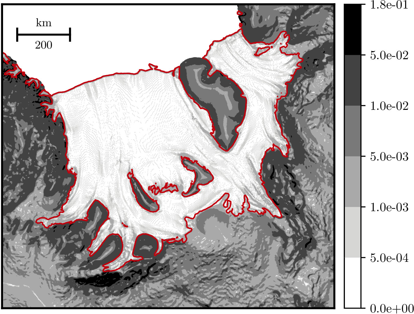
(a) $\|\nabla S\|$

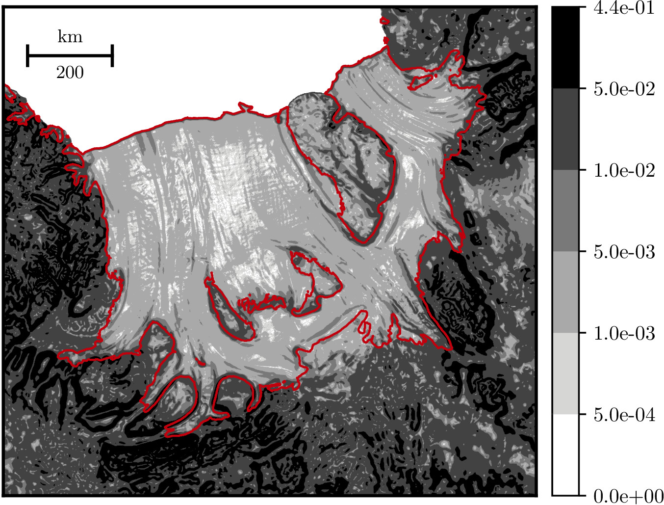
(b) $\|\nabla B\|$

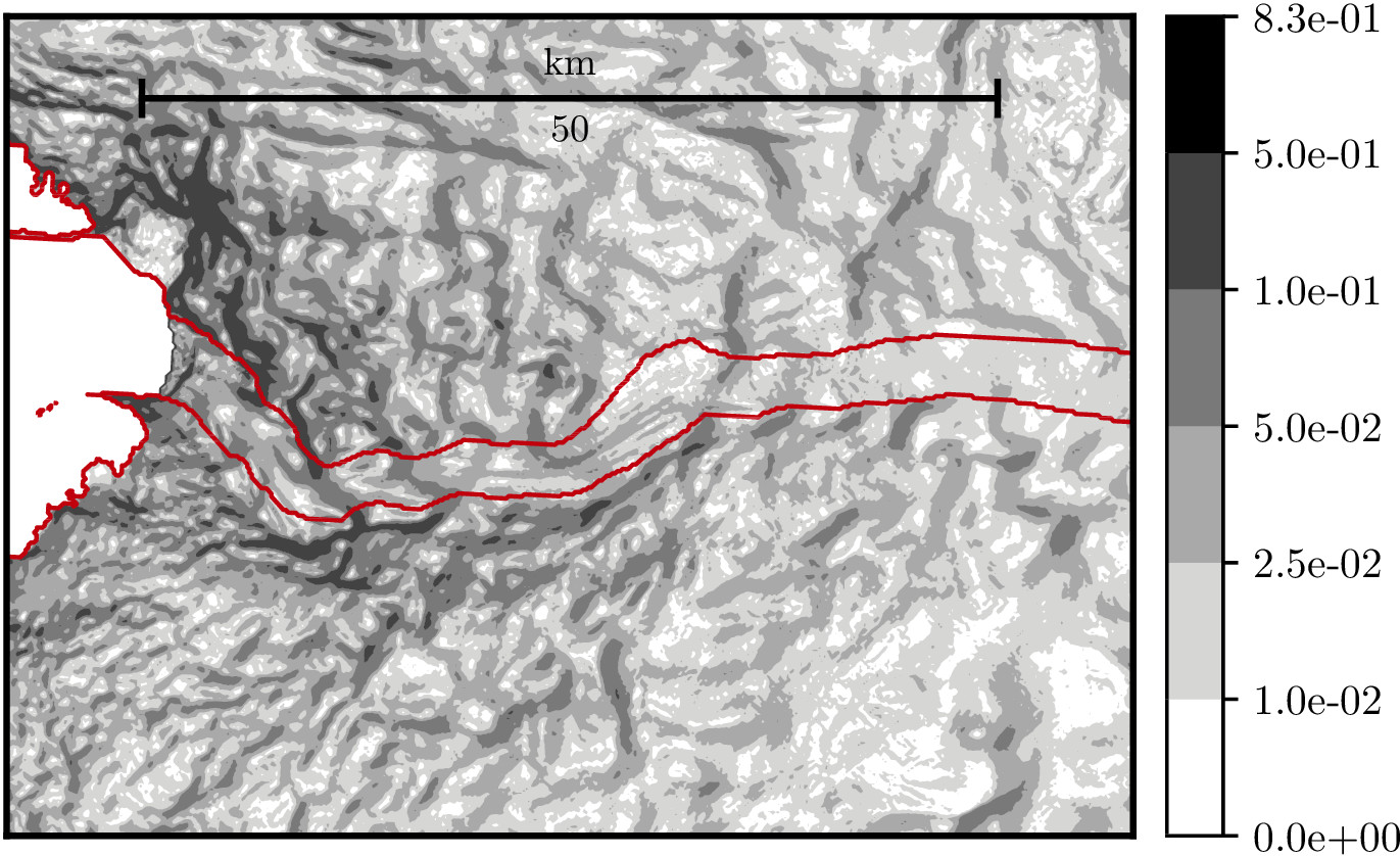
(c) $\|\nabla S\|$

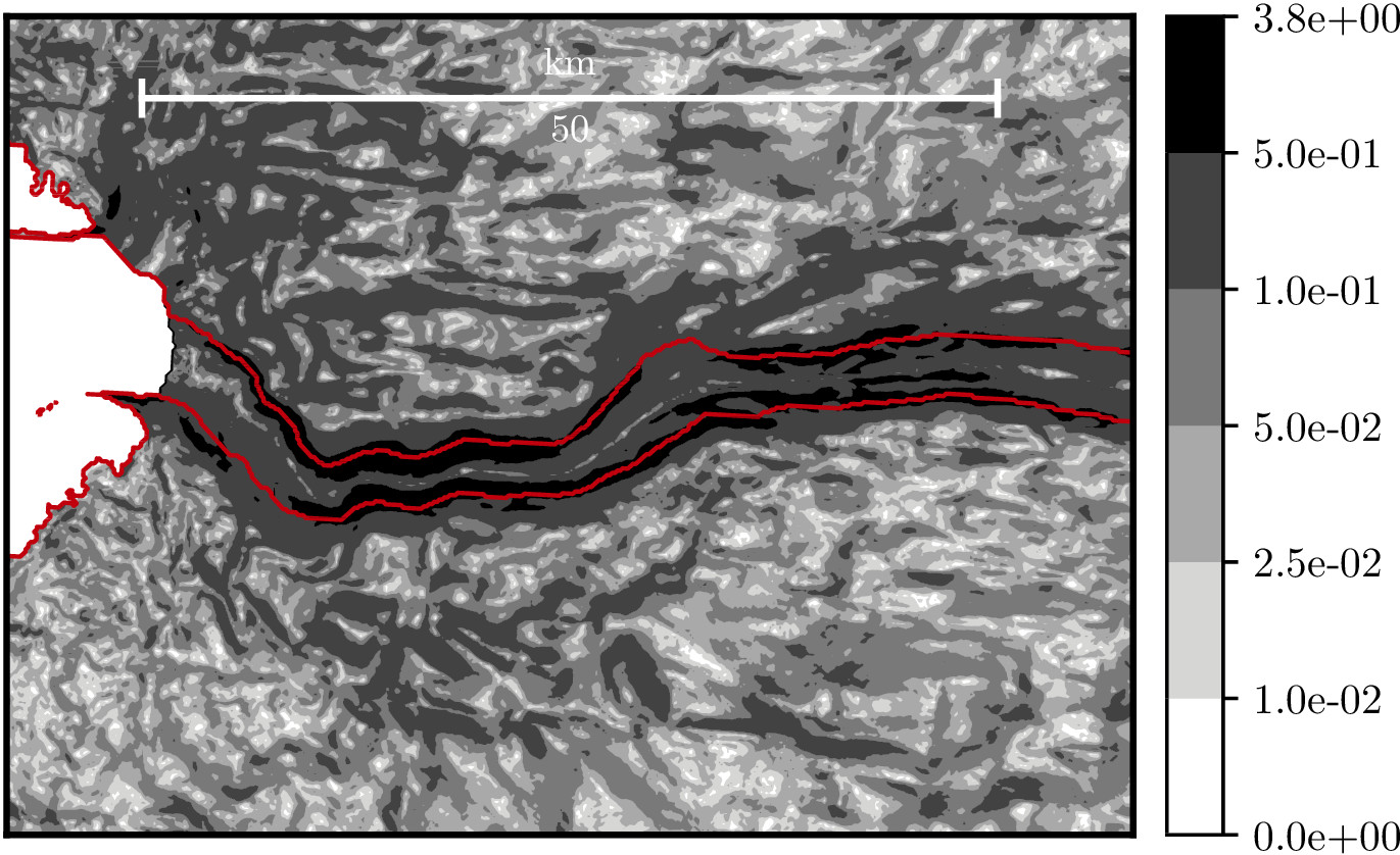
(d) $\|\nabla B\|$

Figure 3: Unitless surface-gradient magnitude of the region surrounding the Filchner-Ronne-ice shelf with topography provided by [9] (top) and region surrounding Jakobshavn glacier with topography provided by [23] (bottom) calculated using methods provided by [14]. For purposes of visualization, a Gaussian filter with 2 km standard deviation has been applied to the Antarctica surfaces $S$ and $B$; the Jakobshavn topography have not been smoothed. The periphery, grounding line, and -500 m depth contour of the main Jakobshavn ice channel are outlined red.

Figure 4: A two-dimensional-ice sheet with domain $\varOmega=[a,b]\times[B,S]$ with uniform accumulation $\mathring{S}>0$ along the upper surface $\varGamma_{\mathrm{S}}$ and $\mathring{B}=0$ over the lower surface $\varGamma_{\mathrm{B}}$. After some interval of time $\Delta t$, a thickness layer of radially-uniform depth will be deposited (left). An identical ice sheet which imposes assumptions Eq. 32 will have a uniform thickness layer in the $z$ direction (right).

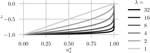
Figure 5: Analytic-$x$ component of velocity $u_{x}^{\mathrm{a}}$ given by Eq. 39 with $S=0$, $B=-1$, $u_{x\mathrm{B}}^{\mathrm{a}}=0$, and $u_{x\mathrm{S}}^{\mathrm{a}}=1$ over a selection of values of deformation parameter $\lambda$.

6 Analytic solution

An analytic solution satisfying incompressibility relation Eq. 24 and free-surface equations Eqs. 27 and 28 provides the ability to verify and thereby guarantee the correct implementation of any numerical model associated with ice-sheet mass conservation. The verification of ice-sheet momentum conservation models using with this velocity in turn makes possible the ability to quantify the effects associated with imposing $\underline{u}\cdot\underline{\hat{n}}=0$ over an impenetrable lower surface with non-zero surface accumulation or ablation (cf. Remark 2.1); assumptions Eq. 32 when solving free-surface relations Eqs. 27 and 28 for an evolving surface $\varGamma$ (cf. Remark 4.2); and assumptions Eq. 32 when inverting quasi-mass-balance relation Eq. 31 (cf. Remark 5.1).

Generalized analytic-velocity solutions proposed heretofore (cf. [34] and [17]) did not incorporate the effects of basal-mass balance $\mathring{B}$ and had been simplified using Eq. 32. Moreover, the boundary condition $\mathring{B}=-\underline{u}\cdot\underline{\hat{n}}$ has not been verified by ice-sheet momentum models up to this time; instead, the essential condition $\underline{u}=\underline{0}$ has been assumed. It was first established by [39] that Galerkin implementations of the Navier boundary conditions converge at a sub-optimal rate. In addition, it was discovered by [37] that numerical results may fail to converge for domains with smooth boundaries for both Galerkin approximation techniques of [26] and [40] which incorporate Navier boundary conditions. The Navier boundary condition is a necessary component for any ice-sheet numerical model which specifies basal sliding. Therefore, the analytic-velocity solution formulated here is the first completely generalized and absolutely mass-conserving velocity for use as verification of momentum conservation and all boundary conditions associated with any two- or three-dimensional ice-sheet numerical model.

Following the procedure of [34] and [17], the vertical component of velocity $u_{z}$ is defined such that kinematic-boundary conditions Eqs. 27 and 28 are linearly interpolated with depth within the ice-sheet domain $\varOmega$. That is, the linearly-interpolated analytic vertical component of velocity is given by

(35) $$u_{z}^{\mathrm{a}}(\underline{x},t)=\xi_{\mathrm{S}}u_{z\mathrm{S}}^{\mathrm{a}}+\xi_{\mathrm{B}}u_{z\mathrm{B}}^{\mathrm{a}},$$

where

(36) $$\xi_{\mathrm{B}}(\underline{x},t)=\frac{S(x,y,t)-z}{H(x,y,t)},\hskip 28.45274pt\xi_{\mathrm{S}}(\underline{x},t)=\frac{z-B(x,y,t)}{H(x,y,t)};$$

and where $u_{z\mathrm{S}}^{\mathrm{a}}=u_{z}^{\mathrm{a}}(x,y,z=S,t)$ and $u_{z\mathrm{B}}^{\mathrm{a}}=u_{z}^{\mathrm{a}}(x,y,z=B,t)$ are given by solving relations Eqs. 27 and 28 for $u_{z}$ at the upper and lower surfaces:

(37) $$u_{z\mathrm{S}}^{\mathrm{a}}(\underline{x},t)= -\|\hat{\underline{k}}-\nabla S\|\mathring{S}+\frac{\partial S}{\partial t}+u_{x}^{\mathrm{a}}\frac{\partial S}{\partial x}+u_{y}^{\mathrm{a}}\frac{\partial S}{\partial y}$$

(38) $$u_{z\mathrm{B}}^{\mathrm{a}}(\underline{x},t)= +\|\nabla B-\hat{\underline{k}}\|\mathring{B}+\frac{\partial B}{\partial t}+u_{x}^{\mathrm{a}}\frac{\partial B}{\partial x}+u_{y}^{\mathrm{a}}\frac{\partial B}{\partial y}.$$

Analytic-velocity components $u_{x}=u_{x}^{\mathrm{a}}(\underline{x},t)$ and $u_{y}=u_{y}^{\mathrm{a}}(\underline{x},t)$ are to be determined in the following analysis.

Remark 6.1.

Analytic-vertical velocity Eq. 35 is a function of the geometry $S(\underline{x},t)$ and $B(\underline{x},t)$ and horizontal-velocity components $u_{x}^{\mathrm{a}}(\underline{x},t)$ and $u_{y}^{\mathrm{a}}(\underline{x},t)$ only. Thus $u_{z}^{\mathrm{a}}$ defined by Eq. 35 is fully determined once $S$, $B$, $u_{x}^{\mathrm{a}}$ and $u_{y}^{\mathrm{a}}$ have been specified.

For simplicity, the $x$ component of velocity is chosen to be

(39) $$u_{x}^{\mathrm{a}}(\underline{x},t) =\left(u_{x\mathrm{S}}^{\mathrm{a}}-u_{x\mathrm{B}}^{\mathrm{a}}\right)\left(1-\xi_{\mathrm{B}}^{\lambda}\right)+u_{x\mathrm{B}}^{\mathrm{a}},$$

where $\lambda\in\mathbb{R}$ controls the magnitude of the $x$-component of velocity with depth, $u_{x\mathrm{B}}^{\mathrm{a}}$ is the $x$ component of velocity at the lower surface $B$, and $u_{x\mathrm{S}}^{\mathrm{a}}$ is the $x$ component of velocity at the upper surface $S$ (Fig. 5).

Remark 6.2.

The value of $u_{x\mathrm{B}}^{\mathrm{a}}$ can be used to prescribe an amount of basal sliding, in turn accommodating the possibility to create a non-zero basal-mass balance $\mathring{B}$ over static lower surfaces—characterized by $\underline{w}\cdot\underline{\hat{n}}=0$ on $\varGamma_{\mathrm{B}}$—as indicated by Eq. 19. Hence this parameter may be used to verify the numerical implementation of the Dirichlet boundary condition $\mathring{B}=-\underline{u}\cdot\underline{\hat{n}}$ over basal surfaces (cf. Remark 2.1).

The final $y$ component of velocity $u_{y}^{\mathrm{a}}$ must satisfy incompressibility relation Eq. 24, i. e.,

(40) $$\frac{\partial u_{x}^{\mathrm{a}}}{\partial x}+\frac{\partial u_{y}^{\mathrm{a}}}{\partial y}+\frac{\partial u_{z}^{\mathrm{a}}}{\partial z} =0.$$

Therefore, taking the derivative of analytic-$z$ velocity Eq. 35 with respect to $z$ results in

$$\frac{\partial u_{z}^{\mathrm{a}}}{\partial z}= +\frac{1}{H}\left(-\|\hat{\underline{k}}-\nabla S\|\mathring{S}-\|\nabla B-\hat{\underline{k}}\|\mathring{B}+\frac{\partial H}{\partial t}+u_{x}^{\mathrm{a}}\frac{\partial H}{\partial x}\right)$$

$$+\left(u_{x\mathrm{S}}^{\mathrm{a}}-u_{x\mathrm{B}}^{\mathrm{a}}\right)\lambda\xi_{\mathrm{B}}^{\lambda}\frac{1}{H}\left(\frac{\xi_{\mathrm{S}}}{\xi_{\mathrm{B}}}\frac{\partial S}{\partial x}+\frac{\partial B}{\partial x}\right)$$

(41) $$+\left(\xi_{\mathrm{S}}\frac{\partial S}{\partial y}+\xi_{\mathrm{B}}\frac{\partial B}{\partial y}\right)\frac{\partial u_{y}^{\mathrm{a}}}{\partial z}+\frac{1}{H}\frac{\partial H}{\partial y}u_{y}^{\mathrm{a}},$$

while differentiation of analytic-$x$ velocity Eq. 39 with respect to $x$ results in

(42) $$\frac{\partial u_{x}^{\mathrm{a}}}{\partial x} =\left(1-\xi_{\mathrm{B}}^{\lambda}\right)\frac{\partial u_{x\mathrm{S}}^{\mathrm{a}}}{\partial x}+\xi_{\mathrm{B}}^{\lambda}\frac{\partial u_{x\mathrm{B}}^{\mathrm{a}}}{\partial x}-\left(u_{x\mathrm{S}}^{\mathrm{a}}-u_{x\mathrm{B}}^{\mathrm{a}}\right)\lambda\xi_{\mathrm{B}}^{\lambda-1}\frac{\partial\xi_{\mathrm{B}}}{\partial x}.$$

Combining mass-conservation relation Eq. 40 with velocity derivatives Sections 6 and 42 produces the linear first-order partial-differential equation for the unknown $y$ component of velocity $u_{y}^{\mathrm{a}}$ (cf. supplementary material Section B.1)

(43) $$A+Gu_{y}^{\mathrm{a}}+\frac{\partial u_{y}^{\mathrm{a}}}{\partial y}+C\frac{\partial u_{y}^{\mathrm{a}}}{\partial z}=0,$$

where

$$A(\underline{x},t)= +\frac{\partial u_{x\mathrm{S}}^{\mathrm{a}}}{\partial x}+\frac{1}{H}\left(\frac{\partial H}{\partial t}+u_{x\mathrm{S}}^{\mathrm{a}}\frac{\partial H}{\partial x}-\|\hat{\underline{k}}-\nabla S\|\mathring{S}-\|\nabla B-\hat{\underline{k}}\|\mathring{B}\right)$$

$$+\frac{(S-z)^{\lambda}}{H^{\lambda}}\left(\frac{\partial u_{x\mathrm{B}}^{\mathrm{a}}}{\partial x}-\frac{\partial u_{x\mathrm{S}}^{\mathrm{a}}}{\partial x}+\left(u_{x\mathrm{S}}^{\mathrm{a}}-u_{x\mathrm{B}}^{\mathrm{a}}\right)\left(\frac{1}{H}\frac{\partial B}{\partial x}\right)\right)$$

$$+\frac{(S-z)^{\lambda-1}\left(z-S\right)}{H^{\lambda+1}}\left(u_{x\mathrm{S}}^{\mathrm{a}}-u_{x\mathrm{B}}^{\mathrm{a}}\right)\frac{\partial S}{\partial x}$$

$$G(x,y,t)= +\frac{1}{H}\frac{\partial H}{\partial y}$$

$$C(\underline{x},t)= +\xi_{\mathrm{S}}\frac{\partial S}{\partial y}+\xi_{\mathrm{B}}\frac{\partial B}{\partial y}.$$

Remark 6.3.

Due to the fact that each of $A$, $G$, and $C$ of equation Eq. 43 are known for all $\underline{x}$ and $t$—and that only the $y$ and $z$ derivatives of $u_{y}^{\mathrm{a}}$ are present—the unknown velocity $u_{y}^{\mathrm{a}}$ is determined solely by its dependence on the $y$ and $z$ coordinates. In addition, as the coefficients $A$, $G$, and $C$ do not depend on $u_{y}^{\mathrm{a}}$, equation Eq. 43 is linear; the authors of [34] and [17] incorrectly describe their analogous relations as quasi linear. Regardless of the classification of the partial-differential equation, the appropriate method used to solve hyperbolic problem Eq. 43 is the method of characteristics (cf. section 3.6.4 of [7]).

Consider a normal vector to a manifold $M$ in the $yz$ plane defined by

(44) $$\underline{n}_{M}(y,z)=\left[\hskip 8.53581pt1\hskip 8.53581ptu_{y}^{\mathrm{a}}(y,z)\hskip 8.53581pt\frac{\partial u_{y}^{\mathrm{a}}}{\partial y}(y,z)\hskip 8.53581pt\frac{\partial u_{y}^{\mathrm{a}}}{\partial z}(y,z)\hskip 8.53581pt\right]^{\intercal}.$$

Problem Eq. 43 can thus be stated equivalently as

(45) $$\underline{n}_{M}\cdot\underline{a}=0,\hskip 28.45274pt\underline{a}=\left[\hskip 5.69054ptA\hskip 5.69054ptG\hskip 5.69054pt1\hskip 5.69054ptC\hskip 5.69054pt\right]^{\intercal}.$$

The manifold $M$ is called invariant if and only if Eq. 45 holds, and in such a case the solution $u_{y}^{\mathrm{a}}$ to Eq. 45 is a solution to partial-differential equation Eq. 43. Hence the following theorem is presented:

Theorem 6.4.

There exists an invariant manifold $M$ such that Eqs. 44 and 45 is a solution to partial-differential equation Eq. 43.

Proof 6.5.

Assume that a curve $s:\mathbb{R}\rightarrow\mathbb{R}^{3}$ in the $yz$ plane exists such that the solution to Eq. 43 may be parameterized by $u_{y}^{\mathrm{a}}(s)=u_{y}^{\mathrm{a}}(y(s),z(s))$. In this case, application of the chain rule (cf. Theorem A.7) produces

$$\frac{\mathrm{d}u_{y}^{\mathrm{a}}}{\mathrm{d}s}=\frac{\partial u_{y}^{\mathrm{a}}}{\partial y}\frac{\mathrm{d}y}{\mathrm{d}s}+\frac{\partial u_{y}^{\mathrm{a}}}{\partial z}\frac{\mathrm{d}z}{\mathrm{d}s}.$$

Comparing this expression with problem Eq. 43 results in the observation that

(46) $$\frac{\mathrm{d}u_{y}^{\mathrm{a}}}{\mathrm{d}s}=A+Gu_{y}^{\mathrm{a}}\hskip 7.11317pt\iff\hskip 7.11317pt\frac{\mathrm{d}y}{\mathrm{d}s}=-1,\hskip 14.22636pt\frac{\mathrm{d}z}{\mathrm{d}s}=-C,$$

and on elimination of $\ \mathrm{d}s$ produces the Lagrange-Charpit equations

(47) $$\mathrm{d}u_{y}^{\mathrm{a}}\left(A+Gu_{y}^{\mathrm{a}}\right)^{-1}\hskip 5.69054pt=\hskip 5.69054pt-\mathrm{d}y\hskip 5.69054pt=\hskip 5.69054pt-\mathrm{d}zC^{-1}.$$

The relationship between the two right-most differential terms of Eq. 47 can be stated as (cf. supplementary material Section B.2) $\partial_{y}\left(z/H\right)=\partial_{y}\left(B/H\right)$, which integrated with respect to $y$ produces for some constant $z_{0}$,

(48) $$\frac{z-B}{H}=\xi_{\mathrm{S}}=z_{0}\hskip 14.22636pt\iff\hskip 14.22636ptz=z_{0}H+B.$$

The relationship between the two left-most differential terms of Eq. 47 can be stated as (cf. supplementary material Section B.3) $\partial_{y}\left(Hu_{y}^{\mathrm{a}}\right)=-HA$, which integrated with respect to $y$ produces for some constant $u_{y0}$,

(49) $$Hu_{y}^{\mathrm{a}}=- \int_{y}HA\ \mathrm{d}y+u_{y0}.$$

The integration constants embedded within Eq. 48 and Eq. 49 provide two invariant coordinates in the $yz$ plane defined by

$$\phi_{1}(y,z)=z_{0}=\xi_{\mathrm{S}}\hskip 28.45274pt\text{and}\hskip 28.45274pt\phi_{2}(y,z)=u_{y0}=Hu_{y}^{\mathrm{a}}+\int_{y}HA\ \mathrm{d}y;$$

therefore, the manifold $M$ of Eq. 45 is invariant.

The horizontal component of velocity $u_{y}^{\mathrm{a}}$ may now be defined by a function $\vartheta=\vartheta(\phi_{1},\phi_{2})$ satisfying $\vartheta(\phi_{1},\phi_{2})=0$. This function may be arbitrarily specified in terms of the coordinates $\phi_{1}$ and $\phi_{2}$; for simplicity, let $\vartheta(\phi_{1},\phi_{2})\equiv\{\phi_{1}(y,z)=0,\ \phi_{2}(y,z)=0\}\iff z_{0}=0,\ u_{y0}=0$. In this case, solving Eq. 49 with $u_{y0}=0$ for $u_{y}^{\mathrm{a}}$ produces

$$u_{y}^{\mathrm{a}}(\underline{x},t)=- \frac{1}{H}\int_{y}\left[H\frac{\partial u_{x\mathrm{S}}^{\mathrm{a}}}{\partial x}+\frac{\partial H}{\partial t}+u_{x\mathrm{S}}^{\mathrm{a}}\frac{\partial H}{\partial x}-\|\hat{\underline{k}}-\nabla S\|\mathring{S}-\|\nabla B-\hat{\underline{k}}\|\mathring{B}\right]\ \mathrm{d}y$$

$$- \left(1-\frac{z-B}{H}\right)^{\lambda}\frac{1}{H}\int_{y}\left[H\left(\frac{\partial u_{x\mathrm{B}}^{\mathrm{a}}}{\partial x}-\frac{\partial u_{x\mathrm{S}}^{\mathrm{a}}}{\partial x}\right)+\left(u_{x\mathrm{S}}^{\mathrm{a}}-u_{x\mathrm{B}}^{\mathrm{a}}\right)\frac{\partial B}{\partial x}\right]\ \mathrm{d}y$$

(50) $$- \left(1-\frac{z-B}{H}\right)^{\lambda-1}\left(\frac{z-B}{H}-1\right)\frac{1}{H}\int_{y}\left[\left(u_{x\mathrm{S}}^{\mathrm{a}}-u_{x\mathrm{B}}^{\mathrm{a}}\right)\frac{\partial S}{\partial x}\right]\ \mathrm{d}y.$$

This completes the derivation of an analytic velocity which satisfies mass conservation relations Eqs. 24, 27, and 28; namely, $\underline{u}^{\mathrm{a}}=[u_{x}^{\mathrm{a}}\ u_{y}^{\mathrm{a}}\ u_{z}^{\mathrm{a}}]^{\intercal}$ with components defined by Eqs. 35, 39, and 6.

Remark 6.6.

The fourth and fifth integrals of Section 6 given by

$$\mathcal{I}_{\mathrm{S}}=\frac{1}{H}\int_{y}\|\hat{\underline{k}}-\nabla S\|\mathring{S}\ \mathrm{d}y\hskip 28.45274pt\text{and}\hskip 28.45274pt\mathcal{I}_{\mathrm{B}}=\frac{1}{H}\int_{y}\|\nabla B-\hat{\underline{k}}\|\mathring{B}\ \mathrm{d}y$$

are elliptic for certain combinations of $S$, $\mathring{S}$, $B$, and $\mathring{B}$. Therefore, in order to derive an elementary representation for Section 6, these functions must be carefully chosen. In particular, this complication will be avoided in the event that the set of functions $\{S,\mathring{S},B,\mathring{B}\}$ are specified to be independent of the $y$ coordinate.

To complete the analysis, expression Section 6 is evaluated at the upper and lower surfaces (cf. supplementary material Section B.4), producing

(51) $$u_{y\mathrm{k}}^{\mathrm{a}}= -\frac{1}{H}\int_{y}\left[\frac{\partial}{\partial x}\left(Hu_{x\mathrm{k}}^{\mathrm{a}}\right)+\frac{\partial H}{\partial t}-\mathring{H}\right]\ \mathrm{d}y,\hskip 14.22636pt\mathrm{k}=\mathrm{S},\mathrm{B},$$

where $\mathring{H}$ is quasi-mass-balance forcing term Eq. 31₂. Finally, once the forms for the parameters have been chosen, the analytic balance velocity (cf. Eq. 29) $\underline{\bar{u}}^{\mathrm{a}}=H^{-1}\int_{B}^{S}\underline{u}^{\mathrm{a}}\ \mathrm{d}z$ can be easily calculated along with the thickness flux

(52) $$\nabla\cdot\left(H\underline{\bar{u}}^{\mathrm{a}}\right)=\underline{\bar{u}}^{\mathrm{a}}\cdot\nabla H+H\nabla\cdot\underline{\bar{u}}^{\mathrm{a}}=\bar{u}_{x}^{\mathrm{a}}\frac{\partial H}{\partial x}+\bar{u}_{y}^{\mathrm{a}}\frac{\partial H}{\partial y}+H\frac{\partial\bar{u}_{x}^{\mathrm{a}}}{\partial x}+H\frac{\partial\bar{u}_{y}^{\mathrm{a}}}{\partial y}.$$

6.1 Example calculation

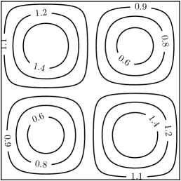
(a) $u_{x\mathrm{S}}^{\mathrm{a}}=u_{x}^{\mathrm{a}}(x,y,z=S)$

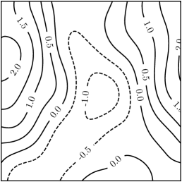
(b) $u_{y\mathrm{S}}^{\mathrm{a}}=u_{y}^{\mathrm{a}}(x,y,z=S)$

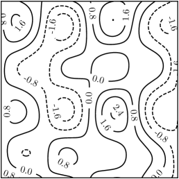
(c) $u_{z\mathrm{S}}^{\mathrm{a}}=u_{z}^{\mathrm{a}}(x,y,z=S)$

(d) $u_{x\mathrm{B}}^{\mathrm{a}}=u_{x}^{\mathrm{a}}(x,y,z=B)$

(e) $u_{y\mathrm{B}}^{\mathrm{a}}=u_{y}^{\mathrm{a}}(x,y,z=B)$

(f) $u_{z\mathrm{B}}^{\mathrm{a}}=u_{z}^{\mathrm{a}}(x,y,z=B)$

(g) $\partial_{t}S$

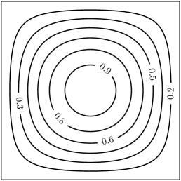
(h) $\partial_{t}B$

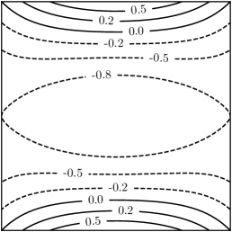
(i) $\partial_{t}H=\partial_{t}S-\partial_{t}B$

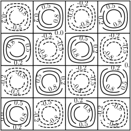
(j) $\mathring{S}$

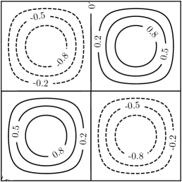
(k) $\mathring{B}$

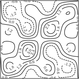
(l) $\nabla\cdot\left(H\underline{\bar{u}}^{\mathrm{a}}\right)$

Figure 6: Inputs and analytic elements generated from relations Eq. 35, Eq. 39, and Section 6 defined over the $xy$ plane with horizontal ($x$-axis) and vertical ($y$-axis) dimensions $\ell=1$.

A specific realization of the solution derived in Section 6 is hereby generated (Fig. 6) over the ice-sheet domain $\varOmega=[0,\ell]\times[0,\ell]\times[B,S]\subset\mathbb{R}^{3}$ with upper and lower surfaces

$$S(x)=\frac{1}{10}\sin\left(\frac{3\pi}{\ell}x\right)\hskip 22.76219pt\text{and}\hskip 22.76219ptB(x)=S(x)-\frac{1}{2}+\frac{1}{10}\sin\left(\frac{2\pi}{\ell}x\right).$$

The sinusoidally-varying $x$ component of velocity at the upper and lower surfaces were chosen to be (Figs. 6a and 6d)

$$u_{x\mathrm{S}}^{\mathrm{a}}=1-\frac{1}{2}\sin\left(\frac{2\pi}{\ell}x\right)\sin\left(\frac{2\pi}{\ell}y\right),\hskip 28.45274ptu_{x\mathrm{B}}^{\mathrm{a}}=\frac{1}{2}-\frac{1}{4}\sin\left(\frac{3\pi}{\ell}x\right)\sin\left(\frac{3\pi}{\ell}y\right).$$

The surface height rate of change at the upper and lower surfaces given respectively by (Figs. 6g and 6h)

$$\frac{\partial S}{\partial t}=3\left(\left(y-\frac{\ell}{2}\right)^{2}-\left(x-\frac{\ell}{2}\right)^{2}\right)\hskip 22.76219pt\text{and}\hskip 22.76219pt\frac{\partial B}{\partial t}=\sin\left(\frac{\pi}{\ell}x\right)\sin\left(\frac{\pi}{\ell}y\right)$$

were chosen in order to generate an ice-sheet domain that is thinning over the interior and thickening in proximity to the $\pm y$ faces (Fig. 6i). Finally, the upper and lower surface-mass balance terms were respectively chosen to be (Figs. 6j and 6k)

$$\mathring{S}=\sin\left(\frac{4\pi}{\ell}x\right)\sin\left(\frac{4\pi}{\ell}x\right)\hskip 22.76219pt\text{and}\hskip 22.76219pt\mathring{B}=\sin\left(\frac{2\pi}{\ell}x\right)\sin\left(\frac{2\pi}{\ell}x\right)$$

in order to optimally demonstrate the flexibility of the manufactured solution.

The analytic velocity components defined by Eqs. 35, 39, and 6 were calculated using the open-source software SymPy [20] (cf. LABEL:r3_script). Choosing $\lambda=2$ and $\ell=1$, the resulting analytic $y$ component of velocity derived from Section 6 at the upper surface (Fig. 6b) and lower surface (Fig. 6e) contains both negative and positive values, with magnitude on the order of the $x$ component of velocity. In addition, periodicity of $u_{x}^{\mathrm{a}}$, $S$, $\partial_{t}S$, $\mathring{S}$, $B$, $\partial_{t}B$, and $\mathring{B}$ are not translated to $u_{y}^{\mathrm{a}}$ or $u_{z}^{\mathrm{a}}$ due to the integration across $y$ used to form Section 6 (Figs. 6c and 6f). Finally, the thickness flux (Fig. 6l) computed from Eq. 52 illustrates the complicated structures in mass flux resulting from incorporation of all aspects of mass conservation for ice sheets.

Remark 6.7.

The fact that the analytic velocity described here is not periodic precludes the possibility of using this solution to verify periodic boundary conditions. However, the input data can be chosen such that the resulting $u_{y}^{\mathrm{a}}$ and therefore also $u_{z}^{\mathrm{a}}$ are periodic. In any case, the lateral-velocity boundary conditions for $u_{y}$ and $u_{z}$ can be specified to correspond with the analytic solutions $u_{y}^{\mathrm{a}}$ and $u_{z}^{\mathrm{a}}$, thereby making possible the verification of mass-conservation relations Eq. 24, Eq. 27, and Eq. 28 within a numerical model; this is the main purpose of this section.

7 Future work

The concepts of mass balance derived here provide the basis of a new formulation for energy and momentum conservation for ice sheets. Once formulated, these concepts will be used to describe conservation laws near the interface of ice and ocean.

Appendix A Mathematical background

Figure 7: Behavior of the Taylor coefficients as $h$ decreases. It is common to refer to the truncated Taylor series which does not include the $h^{n}$ terms as the $\mathrm{n}$th-order-Taylor-series approximation which is clearly only accurate for $h\ll 1$.

This section introduces the relevant mathematical background and definitions utilized throughout the text. For more information regarding higher-dimensional calculus, consult the work of [16]. For more information about general problems in applied mathematics and continuum mechanics, investigate the works of [19] or [33]. An alternative and closely-related continuum-mechanical formulation for ice-sheets has been provided by [12] and expanded upon by [10].

The mathematical theory for discontinuous materials are not as readily available as those for continuous materials; therefore, proofs of pertinent theorems have been deliberated. As such, this section provides a new illustration of the origins of fundamental ice-sheet conservation laws and, moreover, continuum formulations for any discontinuous media. The basis from which we begin is the following fundamental theorem presented by [36]:

Theorem A.1 (Taylor’s theorem).

Any real-valued function $f(x)\in\mathbb{R}$ with $x\in\mathbb{R}$ that is infinitely differentiable about a point $x+h$ with distance $h>0$ may be expressed as the infinite Taylor series

$$f(x+h) =f(x)+f^{\prime}(x)h+\frac{1}{2!}f^{\prime\prime}(x)h^{2}+\frac{1}{3!}f^{\prime\prime\prime}(x)h^{3}+\cdots,$$

where $f^{\prime}(x)$ is the ratio of an infinitesimal change the function $f$ with respect to an infinitesimal change in its coordinate $x$.

Proof A.2.

Consult chapter 9 section 7 of [16].

For scalar variables of multiple coordinates, Theorem A.1 yields the following corollary:

Corollary A.3.

Any multi-dimensional and real-valued function $f(\underline{x})\in\mathbb{R}$ with $\underline{x}\in\mathbb{R}^{n}$ that is infinitely differentiable about a point $\underline{x}+\underline{h}$ where distance vector $\underline{h}$ has magnitude $\|\underline{h}\|>0$ may be expressed as the infinite multi-dimensional Taylor series

$$f(\underline{x}+\underline{h}) =f(\underline{x})+\nabla f(\underline{x})\cdot\underline{h}+\frac{1}{2!}\underline{h}\cdot\nabla^{2}f(\underline{x})\cdot\underline{h}+\cdots\hskip 5.69054pt,$$

where $\nabla f(\underline{x})$ is the gradient of the function $f$ with respect to its coordinates $\underline{x}$.

Recalling that $0<h\neq 0$, rearranging terms of Theorem A.1 and division by $h$ produces

$$\frac{f(x+h)-f(x)}{h}=f^{\prime}(x)+\mathcal{O}(h),$$

which in the limit of small $h$ (Fig. 7) gives rise to the following definitions:

Definition A.4 (Derivative).

The derivative of a real-valued function $f(x)\in\mathbb{R}$ with respect to $x\in\mathbb{R}$ is given by

$$f^{\prime}(x)\equiv\frac{\mathrm{d}f}{\mathrm{d}x}=\lim_{h\rightarrow 0}\left\{\frac{f(x+h)-f(x)}{h}\right\}.$$

Definition A.5 (Partial derivative).

The partial derivative of a real-valued function $f(\underline{x})\in\mathbb{R}$ with respect to $x_{i}\in\underline{x}\in\mathbb{R}^{n}$ is given by

$$\frac{\partial f}{\partial x_{i}}=\lim_{h\rightarrow 0}\left\{\frac{f(x_{1},\ldots,x_{i}+h,\ldots,x_{n})-f(\underline{x})}{h}\right\}.$$

Recalling that Corollary A.3 required that the distance $\|\underline{h}\|>0$, rearranging terms of Corollary A.3 and division by $\|\underline{h}\|$ produces

$$\frac{f(\underline{x}+\underline{h})-f(\underline{x})}{\|\underline{h}\|}=\nabla f(\underline{x})\cdot\hat{\underline{h}}+\mathcal{O}\left(\|\underline{h}\|\right),$$

where $\hat{\underline{h}}=\underline{h}/\|\underline{h}\|$ is a unit vector in the direction $\underline{h}$. Similar to the line of reasoning resulting in Definition A.4, taking the limit of small $\|\underline{h}\|$ suggests the following definition:

Definition A.6 (Gradient).

The gradient of a real-valued function $f(\underline{x})\in\mathbb{R}$ with respect to its vector of coordinates $\underline{x}=[x_{1}\ x_{2}\ \cdots\ x_{n}]^{\intercal}\in\mathbb{R}^{n}$ is given by

$$\frac{\partial f}{\partial\underline{x}} \equiv\nabla f=\left[\frac{\partial f}{\partial x_{1}}\ \frac{\partial f}{\partial x_{2}}\ \cdots\ \frac{\partial f}{\partial x_{n}}\right]^{\intercal}.$$

Theorem A.7 (Chain rule: one independent variable).

Let $f=f(\underline{x})$ be a function composed of $n$ coordinates of a vector $\underline{x}=\underline{x}(t)\in\mathbb{R}^{n}$ each dependent on a single variable $t\in\mathbb{R}$. Then the derivative of $f$ with respect to $t$ is

$$\frac{\mathrm{d}f}{\mathrm{d}t}=\frac{\partial f}{\partial x_{1}}\frac{\mathrm{d}x_{1}}{\mathrm{d}t}+\frac{\partial f}{\partial x_{2}}\frac{\mathrm{d}x_{2}}{\mathrm{d}t}+\cdots+\frac{\partial f}{\partial x_{n}}\frac{\mathrm{d}x_{n}}{\mathrm{d}t}.$$

Proof A.8.

Consult chapter 13 section 5 of [16].

Corollary A.9 (Chain rule: two independent variables).

Let $f=f(\underline{x})$ be a function composed of $n$ coordinates of a vector $\underline{x}=\underline{x}(t,s)\in\mathbb{R}^{n}$ each dependent on two variables $t,s\in\mathbb{R}$. Then the derivative of $f$ with respect to $t$ is

$$\frac{\partial f}{\partial t}=\frac{\partial f}{\partial x_{1}}\frac{\partial x_{1}}{\partial t}+\frac{\partial f}{\partial x_{2}}\frac{\partial x_{2}}{\partial t}+\cdots+\frac{\partial f}{\partial x_{n}}\frac{\partial x_{n}}{\partial t}$$

and the derivative of $f$ with respect to $s$ is

$$\frac{\partial f}{\partial s}=\frac{\partial f}{\partial x_{1}}\frac{\partial x_{1}}{\partial s}+\frac{\partial f}{\partial x_{2}}\frac{\partial x_{2}}{\partial s}+\cdots+\frac{\partial f}{\partial x_{n}}\frac{\partial x_{n}}{\partial s}.$$

Proof A.10.

Consult chapter 13 section 5 of [16].

Remark A.11.

The chain rule for one variable given by Theorem A.7 can be proved by linearizing the Taylor-series expansion of a function $f(\underline{x}(t),t)$ about a point $t+\Delta t$; it is important to note that it is invariant with the choice of coordinate system and therefore provides a measure of total variance of a function with respect to an independent variable, commonly time. Similarly, the chain rule for two variables given by Corollary A.9 can be proved by linearizing the Taylor-series expansion of a function $f(\underline{x}(s,t),s,t)$ about the points $t+\Delta t$ and $s+\Delta s$.

Remark A.12.

The chain rule for one independent variable is widely used in the field of continuum mechanics, which specifies that a variable $F=F(\underline{h},t)$ in the Lagrangian frame of reference defined from an initial-coordinate vector $\underline{h}$ at time $t=0$ has a counterpart $f=f(\underline{x},t)$ in the Eulerian frame at the current-coordinate vector $\underline{x}=\underline{x}(\underline{h},t)$. In addition, the function $\underline{x}$ is defined such that a continuously-differentiable mapping back to initial coordinate $\underline{h}$ exists for all $t$, thereby ensuring that $\underline{x}(\underline{h},t)$ may be inverted for the vector function $\underline{h}=\underline{h}(\underline{x},t)$. Therefore, $F(\underline{h},t)=f(\underline{x}(\underline{h},t),t)$. and $f(\underline{x},t)=F(\underline{h}(\underline{x},t),t)$. Using the fact that the value of $\underline{h}=\underline{h}(\underline{x},t)$ will be identical at each instant $t$, the derivative of the function $F$ with respect to $t$ is given simply by

$$\frac{\mathrm{d}F}{\mathrm{d}t}=\dot{F}(t).$$

However, the position of a point in the continuum will vary with time, and so $\underline{x}=\underline{x}(t)$. Therefore, the derivative of the function $f$ with respect to $t$ is in this case given by

$$\frac{\mathrm{d}f}{\mathrm{d}t}=\dot{f}(\underline{x},t)=\frac{\partial f}{\partial t}\frac{\mathrm{d}t}{\mathrm{d}t}+\frac{\partial f}{\partial\underline{x}}\frac{\mathrm{d}\underline{x}}{\mathrm{d}t},$$

which taken in combination with scalar-gradient Definition A.6 and velocity-vector $\dot{\underline{x}}=\underline{u}=\left[\dot{x}\ \dot{y}\ \dot{z}\right]^{\intercal}$ suggest the notation

$$\dot{f} =\frac{\partial f}{\partial t}+\underline{u}\cdot\nabla f.$$

This relation has been used often enough that it has been given many other names, including the substantial, convective, Lagrangian, material or total derivative, among others. Additionally, the complete change in the state of $f$ described by the relation $\dot{f}$ is referred to as convection; for example, Fourier’s law of heat conduction is specified with a second-order diffusion operator $\mathcal{L}$ such that $\dot{f}=\mathcal{L}u$, and so convection encompasses both advective and diffusive processes. Finally, the literature commonly refers to the second term $\underline{u}\cdot\nabla f$ as the advective component due to the fact that it is responsible for the transport of the quantity $f$ at speed $\underline{u}$.

Theorem A.13 (First fundamental theorem of calculus).

If a given function $f(x)$ is continuous within a closed interval $[a,b]$ and $F(x)$ is an anti-derivative or indefinite integral of $f(x)$, then

$$\int_{a}^{b}f(x)\ \mathrm{d}x=F(b)-F(a).$$

Proof A.14.

Consult chapter 4 section 4 of [16].

Theorem A.15 (Second fundamental theorem of calculus).

If $f(x)$ is a continuous function within an open interval $(a,b)$, an anti-derivative or indefinite integral $F(x)$ is defined as

$$F(x)=\int_{a}^{x}f(t)\ \mathrm{d}t\hskip 14.22636pt\text{with inverse}\hskip 14.22636pt\frac{\mathrm{d}F}{\mathrm{d}x}=f(x)$$

at each point in $x\in(a,b)$.

Proof A.16.

Consult chapter 4 section 4 of [16].

The ice-sheet surface can be completely described using the following theorem:

Theorem A.17 (Gradient of an implicit surface is normal to boundary).

Consider a differentiable surface $\varGamma=\varGamma(\underline{x})\in\mathbb{R}^{3}$ with curvature entirely represented by a differentiable function $z=S(x,y)\in\mathbb{R}^{2}$ with tangent surface $\nabla S$ in the $xy$ plane. The surface $\varGamma$ can be represented implicitly as

$$F(\underline{x})=\left|z-S(x,y)\right|=0=\begin{cases}S(x,y)-z=0\\ z-S(x,y)=0\end{cases},$$

and possesses the property that $\nabla F\cdot\nabla S=0$; that is, the gradient of $F$ is normal to the surface $S$.

Proof A.18.

Let the vector-valued function $\underline{s}=\underline{s}(\underline{x}(t))$ represent an arbitrary curve lying on the surface $z=S(x,y)$ for all $t$. Then $F(\underline{s}(t))=0$ for all $t$ and application of the chain rule (cf. Theorem A.7) yields

$$\frac{\mathrm{d}F}{\mathrm{d}t}= \frac{\partial F}{\partial x}\frac{\mathrm{d}x}{\mathrm{d}t}+\frac{\partial F}{\partial y}\frac{\mathrm{d}y}{\mathrm{d}t}+\frac{\partial F}{\partial z}\frac{\mathrm{d}z}{\mathrm{d}t}=0.$$

Using the facts that $\mathrm{d}_{t}x=\partial_{x}S$, $\mathrm{d}_{t}y=\partial_{y}S$, and $\mathrm{d}_{t}z=\partial_{z}S=0$, gradient notation $\nabla f=[\partial_{x}f\ \partial_{y}f\ \partial_{z}f]^{\intercal}$ (cf. Definition A.6) yields Theorem A.17.

When the boundary $\varGamma$ of a volume $\varOmega$ can be decomposed into two surfaces, one coordinate can be eliminated from the normal vector using Theorem A.17, as follows:

Definition A.19 (Outward-pointing unit-normal vector).

Consider a body $\varOmega(\underline{x},t)\in\mathbb{R}^{3}$ with differentiable surface $\varGamma=\partial\varOmega(\underline{x},t)$ composed of two surfaces $\varGamma_{\mathrm{S}}$ and $\varGamma_{\mathrm{B}}$ where $\varGamma_{\mathrm{S}}\cup\varGamma_{\mathrm{B}}=\varGamma$ and $\varGamma_{\mathrm{S}}\cap\varGamma_{\mathrm{B}}=\emptyset$. Decompose $\varGamma$ using intrinsically-defined upper and lower surfaces (cf. Theorem A.17)

$$F_{\mathrm{S}}(\underline{x},t)=z-S(x,y,t)=0\hskip 14.22636pt\text{and}\hskip 14.22636ptF_{\mathrm{B}}(\underline{x},t)=B(x,y,t)-z=0$$

for some pair of functions $S,B\in\mathbb{R}^{2}$ defined such that $B\leq S$ for all $x$, $y$, and $t$. It follows that the gradient of the upper and lower surface at any instant $t$ is given by $\nabla F_{\mathrm{S}}=\hat{\underline{k}}-\nabla S$ and $\nabla F_{\mathrm{B}}=\nabla B-\hat{\underline{k}}$, where $\hat{\underline{k}}$ is the unit vector pointing in the direction of increasing $z$ coordinate. The outward-pointing unit-normal vectors over these surfaces are respectively

$$\underline{\hat{n}}_{\mathrm{S}}=\frac{\nabla F_{\mathrm{S}}}{\|\nabla F_{\mathrm{S}}\|}\hskip 28.45274pt\text{and}\hskip 28.45274pt\underline{\hat{n}}_{\mathrm{B}}=\frac{\nabla F_{\mathrm{B}}}{\|\nabla F_{\mathrm{B}}\|},$$

with gradient magnitudes given by the $L^{2}(\varGamma)$ norm; i. e.,

$$\|\nabla F_{\mathrm{S}}(\underline{x})\| =\left(\hat{\underline{k}}\cdot\hat{\underline{k}}-2\hat{\underline{k}}\cdot\nabla S+\nabla S\cdot\nabla S\right)^{\frac{1}{2}}=\left(1+\left(\frac{\partial S}{\partial x}\right)^{2}+\left(\frac{\partial S}{\partial y}\right)^{2}\right)^{\frac{1}{2}}$$

$$\|\nabla F_{\mathrm{B}}(\underline{x})\| =\left(\nabla B\cdot\nabla B-2\hat{\underline{k}}\cdot\nabla B+\hat{\underline{k}}\cdot\hat{\underline{k}}\right)^{\frac{1}{2}}=\left(1+\left(\frac{\partial B}{\partial x}\right)^{2}+\left(\frac{\partial B}{\partial y}\right)^{2}\right)^{\frac{1}{2}},$$

where $\partial_{z}S=\partial_{z}B=0$ and $\hat{\underline{k}}\cdot\hat{\underline{k}}=1$ has been used.

The following theorem illuminates the fact that the implicit surface-gradient norms defined in Definition A.19 are integral to the concept of surface area:

Theorem A.20 (Area of an implicit surface).

For a continuous and differentiable function $S=S(x,y)\in\mathbb{R}^{2}$ defined within a region $R$ in the $xy$ plane, the area of the surface $S$ given by the implicit surface defined by Theorem A.17 is

$$A=\int_{R}\ \mathrm{d}S=\int_{R}\|\hat{\underline{k}}-\nabla S\|\ \mathrm{d}R\approx\sum_{i=1}^{n}\|\hat{\underline{k}}-\nabla S_{i}\|\Delta x_{i}\Delta y_{i},$$

for a discretization of $R$ into $n$ rectangles with dimensions $\Delta x_{i}$ and height $\Delta y_{i}$ for all $i=1,2,\ldots,n$.

Proof A.21.

A region $A_{i}$ of an arbitrary parallelogram $i$ of the surface discretization $S$ defined in Theorem A.20 have sides given by the vectors $\underline{u}_{i}=\begin{bmatrix}\Delta x_{i}&0&\Delta x_{i}\partial_{x}S_{i}\end{bmatrix}^{\intercal}$, and $\underline{v}_{i}=\begin{bmatrix}0&\Delta y_{i}&\Delta y_{i}\partial_{y}S_{i}\end{bmatrix}^{\intercal}$. Hence the area of $A_{i}$ is given by

$$\|\underline{u}_{i}\times\underline{v}_{i}\|=\left(1+\left(\frac{\partial S_{i}}{\partial x}\right)^{2}+\left(\frac{\partial S_{i}}{\partial y}\right)^{2}\right)^{\frac{1}{2}}\Delta x_{i}\Delta y_{i}.$$

Using the normal-vector magnitude of Definition A.19, summing over all $i$ parallelograms, and taking the limit as $\Delta x_{i},\Delta y_{i}\rightarrow 0$ produces Theorem A.20.

Theorem A.22 (Leibniz’s rule).

Leibniz formula, referred to as Leibniz’s rule for differentiating an integral with respect to a parameter that appears in the integrand and in the limits of integration, states that if $f(x,y)$ and $\partial_{x}f(x,y)$ are both continuous over the finite domain $y\in[a(x),b(x)]$,

$$\frac{\mathrm{d}}{\mathrm{d}x}\int_{a(x)}^{b(x)}f(x,y)\ \mathrm{d}y =\int_{a(x)}^{b(x)}\frac{\partial f}{\partial x}(x,y)\ \mathrm{d}y+f(x,b(x))\frac{\mathrm{d}b}{\mathrm{d}x}-f(x,a(x))\frac{\mathrm{d}a}{\mathrm{d}x}.$$

Proof A.23.

Let

$$\mathcal{I}(x,a(x),b(x))=\int_{a(x)}^{b(x)}f(x,y)\ \mathrm{d}y.$$

Using one-variable chain rule Theorem A.7, the derivative of $\mathcal{I}$ with respect to $x$ is

$$\frac{\mathrm{d}\mathcal{I}}{\mathrm{d}x}=\frac{\partial\mathcal{I}}{\partial x}\frac{\mathrm{d}x}{\mathrm{d}x}+\frac{\partial\mathcal{I}}{\partial a}\frac{\mathrm{d}a}{\mathrm{d}x}+\frac{\partial\mathcal{I}}{\partial b}\frac{\mathrm{d}b}{\mathrm{d}x}.$$

Next, due to the fact that integration is performed over the coordinate $y$, the linear operations of partial-$x$ differentiation and integration over $y$ may be safely exchanged. That is,

$$\frac{\partial\mathcal{I}}{\partial x} =\lim_{\Delta x\rightarrow 0}\frac{1}{\Delta x}\left(\int_{a(x)}^{b(x)}f(x+\Delta x,y)\ \mathrm{d}y-\int_{a(x)}^{b(x)}f(x,y)\ \mathrm{d}y\right)$$

$$=\lim_{\Delta x\rightarrow 0}\int_{a(x)}^{b(x)}\left(\frac{f(x+\Delta x,y)-f(x,y)}{\Delta x}\right)\ \mathrm{d}y=\int_{a(x)}^{b(x)}\frac{\partial f}{\partial x}(x,y)\ \mathrm{d}y.$$

Next, using first fundamental theorem of calculus Theorem A.13, if $F(x,y)$ is the indefinite integral of $f(x,y)$ with respect to $y$ on $y\in[a,b]$,

$$\frac{\partial\mathcal{I}}{\partial a} =\frac{\partial}{\partial a}\Big{[}F(x,b(x))-F(x,a(x))\Big{]}=-\frac{\partial}{\partial a}F(x,a(x))$$

$$\frac{\partial\mathcal{I}}{\partial b} =\frac{\partial}{\partial b}\Big{[}F(x,b(x))-F(x,a(x))\Big{]}=+\frac{\partial}{\partial b}F(x,b(x)),$$

and using second fundamental theorem of calculus Theorem A.15,

$$\left.\frac{\partial}{\partial a}F(x,y)\right|_{y=a} =\left(\frac{\partial F}{\partial y}\frac{\partial y}{\partial a}\right)_{y=a}=f(x,a(x))$$

$$\left.\frac{\partial}{\partial b}F(x,y)\right|_{y=b} =\left(\frac{\partial F}{\partial y}\frac{\partial y}{\partial b}\right)_{y=b}=f(x,b(x)).$$

Combining the above relations results in Theorem A.22.

Corollary A.24 (Leibniz’s rule for two independent variables).

If a function $f=f(x,y,z)$ and $\partial_{x}f$ are both continuous over a finite domain $z\in[a(x,y),b(x,y)]$,

$$\frac{\partial}{\partial x}\int_{a(x,y)}^{b(x,y)}f(x,y,z)\ \mathrm{d}z= +\int_{a(x,y)}^{b(x,y)}\frac{\partial f}{\partial x}(x,y,z)\ \mathrm{d}z$$

$$+f(x,y,b(x,y))\frac{\partial b}{\partial x}-f(x,y,a(x,y))\frac{\partial a}{\partial x}.$$

Proof A.25.

Let

$$\mathcal{I}(x,y,a(x,y),b(x,y))=\int_{a(x,y)}^{b(x,y)}f(x,y,z)\ \mathrm{d}z.$$

Using the one-variable chain rule (cf. Theorem A.7), the derivative of $\mathcal{I}$ with respect to $x$ is

$$\frac{\mathrm{d}\mathcal{I}}{\mathrm{d}x}= \frac{\partial\mathcal{I}}{\partial x}\frac{\mathrm{d}x}{\mathrm{d}x}+\frac{\partial\mathcal{I}}{\partial y}\frac{\mathrm{d}y}{\mathrm{d}x}+\frac{\partial\mathcal{I}}{\partial a}\frac{\mathrm{d}a}{\mathrm{d}x}+\frac{\partial\mathcal{I}}{\partial b}\frac{\mathrm{d}b}{\mathrm{d}x}.$$

Due to the fact that integration is performed over the coordinate $z$, the linear operations of partial-$x$ differentiation and integration over $z$ may be safely exchanged (cf. Theorem A.22), such that

$$\frac{\partial\mathcal{I}}{\partial x} =\int_{a(x,y)}^{b(x,y)}\frac{\partial f}{\partial x}(x,y,z)\ \mathrm{d}y.$$

Using the first fundamental theorem of calculus (cf. Theorem A.13), if $F(x,y,z)$ is the indefinite integral of $f(x,y,z)$ with respect to $z$ over $z\in[a,b]$,

$$\frac{\partial\mathcal{I}}{\partial a} =\frac{\partial}{\partial a}\Big{[}F(x,y,b))-F(x,y,a)\Big{]}=-\frac{\partial}{\partial a}F(x,y,a)$$

$$\frac{\partial\mathcal{I}}{\partial b} =\frac{\partial}{\partial b}\Big{[}F(x,y,b))-F(x,y,a)\Big{]}=+\frac{\partial}{\partial b}F(x,y,b),$$

and using the second fundamental theorem of calculus (cf. Theorem A.15),

$$\left.\frac{\partial}{\partial a}F(x,y,z)\right|_{z=a} =\left(\frac{\partial F}{\partial z}\frac{\partial z}{\partial a}\right)_{z=a}=f(x,y,a(x,y))$$

$$\left.\frac{\partial}{\partial b}F(x,y,z)\right|_{z=b} =\left(\frac{\partial F}{\partial z}\frac{\partial z}{\partial b}\right)_{z=b}=f(x,y,b(x,y)).$$

Combining the above relations with the facts that $\mathrm{d}_{x}y=0$, $\mathrm{d}_{x}b=\partial_{x}b$, $\mathrm{d}_{x}a=\partial_{x}a$, and $\mathrm{d}_{x}\mathcal{I}=\partial_{x}\mathcal{I}$ produces Corollary A.24.

Theorem A.26 (Divergence theorem).

The integral of the divergence of a differentiable-vector-field $\underline{j}$ within an open and bounded volume $\varOmega=\varOmega(\underline{x})$ is equal to the integral of the outward flux of the vector field across the surface of the volume $\partial\varOmega=\varGamma(\underline{x})$:

$$\int_{\varOmega}\nabla\cdot\underline{j}\ \mathrm{d}\varOmega=\int_{\varGamma}\underline{j}\cdot\underline{\hat{n}}\ \mathrm{d}\varGamma.$$

Proof A.27.

Consult chapter 15 section 7 of [16].

Theorem A.28 (Reynolds transport theorem).

Within an arbitrary time-evolving volume $\varOmega=\varOmega(\underline{x},t)\in\mathbb{R}^{3}$ with boundary $\partial\varOmega=\varGamma(\underline{x},t)$, Leibniz’s rule in three dimensions—better known in continuum mechanics as Reynolds transport theorem [31]—states that for a given continuous quantity $\phi$,

$$\frac{\mathrm{d}}{\mathrm{d}t}\int_{\varOmega(t)}\phi\ \mathrm{d}\varOmega(t)=\int_{\varOmega(t)}\frac{\partial\phi}{\partial t}\ \mathrm{d}\varOmega(t)+\int_{\varGamma(t)}\phi\underline{w}\cdot\underline{\hat{n}}\ \mathrm{d}\varGamma(t),$$

where $\underline{w}$ is the velocity of surface $\varGamma$ and $\underline{\hat{n}}$ is the outward-facing unit-normal vector for $\varGamma$.

Proof A.29.

Consult chapter III section 4 of [33].

Corollary A.30.

If the volume defined in Theorem A.28 remains constant—i. e., if $\varOmega=\varOmega(\underline{x})$, $\partial\varOmega=\varGamma(\underline{x})$ and $\underline{w}=\underline{0}$—Reynolds-transport Theorem A.28 reduces to

$$\frac{\mathrm{d}}{\mathrm{d}t}\int_{\varOmega}\phi\ \mathrm{d}\varOmega=\int_{\varOmega}\frac{\partial\phi}{\partial t}\ \mathrm{d}\varOmega.$$

Proof A.31.

Time-invariant volumes are characterized by $\underline{w}=\underline{0}$ on $\varGamma$ and therefore $\int_{\varGamma}\phi\underline{w}\cdot\underline{\hat{n}}\ \mathrm{d}\varGamma=0$; this expression applied to Theorem A.28 yields Corollary A.30.

Definition A.32 (Fundamental conservation equation).

Consider an arbitrary fixed volume $\varOmega^{\mathrm{e}}=\varOmega^{\mathrm{e}}(\underline{x})\subset\varOmega(\underline{x},t)$ with boundary $\partial\varOmega^{\mathrm{e}}=\varGamma^{\mathrm{e}}(\underline{x})$ and quantity $\phi=\phi(\underline{x},t)$. Then

$$\begin{matrix}\text{the total}\\ \text{rate of change}\\ \text{of quantity $\phi$}\\ \text{in $\varOmega^{\mathrm{e}}$}\end{matrix}\hskip 7.11317pt=\hskip 7.11317pt\begin{matrix}\text{the inward flux}\\ \text{of $\phi$ across the}\\ \text{boundary $\varGamma^{\mathrm{e}}$}\\ \end{matrix}\hskip 7.11317pt+\hskip 7.11317pt\begin{matrix}\text{the generation}\\ \text{of quantity $\phi$}\\ \text{within $\varOmega^{\mathrm{e}}$}\end{matrix},$$

or mathematically, the fundamental-conservation equation

$$\frac{\mathrm{d}}{\mathrm{d}t}\int_{\varOmega^{e}}\phi\ \mathrm{d}\varOmega^{\mathrm{e}}=-\int_{\varGamma^{\mathrm{e}}}\left(\phi\underline{u}+\underline{j}\right)\cdot\underline{\hat{n}}\ \mathrm{d}\varGamma^{\mathrm{e}}+\int_{\varOmega^{\mathrm{e}}}\mathring{f}\ \mathrm{d}\varOmega^{\mathrm{e}},$$

with volumetric-source term $\mathring{f}$, material velocity $\underline{u}$, advective flux $\phi\underline{u}$, non-advective flux $\underline{j}$, and outward-pointing unit-normal vector $\underline{\hat{n}}$.

Definition A.33 (Differential continuity equation in conservative form).

Provided that the quantity $\phi$ is differentiable, applying Reynolds transport Corollary A.30 to the time-derivative term and divergence Theorem A.26 to the surface integral of Definition A.32 results in

$$\int_{\varOmega^{\mathrm{e}}}\frac{\partial\phi}{\partial t}\ \mathrm{d}\varOmega^{\mathrm{e}}+\int_{\varOmega^{\mathrm{e}}}\nabla\cdot\left(\phi\underline{u}+\underline{j}\right)\ \mathrm{d}\varOmega^{\mathrm{e}} =\int_{\varOmega^{\mathrm{e}}}\mathring{f}\ \mathrm{d}\varOmega^{\mathrm{e}}.$$

Therefore, due to the fact that the domain $\varOmega^{\mathrm{e}}\subset\varOmega$ was taken arbitrarily and by linearity of the integral operator, the continuity equation in conservative form is given by

$$\frac{\partial\phi}{\partial t}+\nabla\cdot\left(\phi\underline{u}+\underline{j}\right)=\mathring{f} \text{in }\varOmega.$$

Definition A.34 (Differential continuity equation in non-conservative form).

The advective-flux divergence term in Definition A.33 can be expanded using the differential-product rule to

$$\frac{\partial\phi}{\partial t}+\underline{u}\cdot\nabla\phi+\phi\nabla\cdot\underline{u}+\nabla\cdot\underline{j}=\mathring{f} \text{in }\varOmega.$$

This can be then be reduced by applying chain rule Theorem A.7 to get the continuity equation in non-conservative form

$$\frac{\mathrm{d}\phi}{\mathrm{d}t}+\phi\nabla\cdot\underline{u}+\nabla\cdot\underline{j}=\mathring{f} \text{in }\varOmega.$$

Continuity equation Definition A.33 is so named for the fact that in its derivation the quantity $\phi$ had been required to not contain discontinuities within the domain $\varOmega$; this is needed in order to apply the divergence theorem (cf. Theorem A.26) which is applicable for continuous material properties only. In addition, while the integral statement of conservation used in its derivation (cf. Definition A.32) does not utilize the divergence theorem and thus does not require the material be continuous within $\varOmega$, additional theory is required in order to state an analogous integral relation for discontinuous media. Materials which contain discontinuous properties are characterized by singular surfaces; these are the interfaces across which a jump in material properties exists. The following operator will simplify future notation:

Definition A.35 (Jump discontinuity).

Consider a volume $\varOmega^{-}=\varOmega^{-}(\underline{x})\in\mathbb{R}^{3}$ with boundary $\varGamma^{-}=\partial\varOmega^{-}(\underline{x})$ and outward-pointing unit-normal vector $\underline{\hat{n}}^{-}$ in contact with another volume $\varOmega^{+}=\varOmega^{+}(\underline{x})\in\mathbb{R}^{3}$ with boundary $\varGamma^{+}=\partial\varOmega^{+}(\underline{x})$ and outward-pointing unit-normal vector $\underline{\hat{n}}^{+}$ (cf. Fig. 1). The jump of a scalar quantity $\phi=\phi(\underline{x})$ and vector quantity $\underline{\phi}=\underline{\phi}(\underline{x})$ across the shared boundary $\varSigma=\varGamma^{+}\cap\varGamma^{-}$ are respectively

$$\left\llbracket{\phi}\right\rrbracket=\phi^{-}\underline{\hat{n}}^{-}+\phi^{+}\underline{\hat{n}}^{+}\hskip 28.45274pt\text{and}\hskip 28.45274pt\left\llbracket{\underline{\phi}}\right\rrbracket=\underline{\phi}^{-}\cdot\underline{\hat{n}}^{-}+\underline{\phi}^{+}\cdot\underline{\hat{n}}^{+},$$

where the normal vectors satisfy $\underline{\hat{n}}^{+}=-\underline{\hat{n}}^{-}$ for all $\underline{x}\in\varSigma$.

Hence a scalar material property $\phi$ is discontinuous across a surface $\varSigma$ when $\left\llbracket{\phi}\right\rrbracket\neq 0$. Jump discontinuity Definition A.35 can be used to neatly describe the divergence theorem for discontinuous media, as follows:

Theorem A.36 (Discontinuous divergence).

The integral of the divergence of a vector field $\underline{j}=\underline{j}(\underline{x},t)$ possessing a discontinuity along a surface $\varSigma$ within an open and bounded volume $\varOmega=\varOmega(\underline{x},t)$ with exterior surface $\varGamma$ is given by

$$\int_{\varGamma}\underline{j}\cdot\underline{\hat{n}}\ \mathrm{d}\varGamma=\int_{\varOmega}\nabla\cdot\underline{j}\ \mathrm{d}\varOmega-\int_{\varSigma}\left\llbracket{\underline{j}}\right\rrbracket\ \mathrm{d}\varSigma,$$

where the jump operator $\left\llbracket{\cdot}\right\rrbracket$ is given by Definition A.35.

Proof A.37.

Applying the continuous divergence theorem (cf. Theorem A.26) to both regions and taking the sum yields

$$\int_{\varOmega}\left(\nabla\cdot\underline{j}^{-}+\nabla\cdot\underline{j}^{+}\right)\ \mathrm{d}\varOmega=\int_{\varGamma}\left(\underline{j}^{-}\cdot\underline{\hat{n}}^{-}+\underline{j}^{+}\cdot\underline{\hat{n}}^{+}\right)\ \mathrm{d}\varGamma+\int_{\varSigma}\left(\underline{j}^{-}\cdot\underline{\hat{n}}^{-}+\underline{j}^{+}\cdot\underline{\hat{n}}^{+}\right)\ \mathrm{d}\varSigma.$$

Making use of the facts that $\underline{j}^{+}=\underline{0}$ in $\overline{\varOmega^{-}}$, and $\underline{j}^{-}=\underline{0}$ in $\overline{\varOmega^{+}}$,

$$\int_{\varOmega}\nabla\cdot\underline{j}\ \mathrm{d}\varOmega=\int_{\varGamma}\underline{j}\cdot\underline{\hat{n}}\ \mathrm{d}\varGamma+\int_{\varSigma}\left(\underline{j}^{-}\cdot\underline{\hat{n}}^{-}+\underline{j}^{+}\cdot\underline{\hat{n}}^{+}\right)\ \mathrm{d}\varSigma.$$

Finally, applying jump discontinuity Definition A.35 and rearranging terms results in Theorem A.36.

Discontinuous divergence Theorem A.36 may be used to relate the total rate of change of an integrated quantity which contains an evolving discontinuity surface via the following theorem:

Theorem A.38 (Generalized Reynolds transport).

Within an arbitrary time-evolving volume $\varOmega=\varOmega(\underline{x},t)$ with exterior surface $\varGamma$, a quantity $\phi=\phi(\underline{x},t)$ discontinuous across a surface $\varSigma\in\varOmega$ will obey

$$\frac{\mathrm{d}}{\mathrm{d}t}\int_{\varOmega}\phi\ \mathrm{d}\varOmega=\int_{\varOmega}\frac{\partial\phi}{\partial t}\ \mathrm{d}\varOmega+\int_{\varGamma}\phi\underline{w}\cdot\underline{\hat{n}}\ \mathrm{d}\varGamma+\int_{\varSigma}\left\llbracket{\phi\underline{w}}\right\rrbracket\ \mathrm{d}\varSigma,$$

where $\underline{w}=\underline{w}(\underline{x},t)$ is the propagation velocity of exterior surface $\varGamma$ and discontinuity surface $\varSigma$; vector $\underline{\hat{n}}$ is the outward-facing-unit normal; and the jump operator $\left\llbracket{\cdot}\right\rrbracket$ is given by Definition A.35.

Proof A.39.

Applying the continuous form of Reynolds transport theorem (cf. Theorem A.28) to both regions and taking the sum results in

$$\frac{\mathrm{d}}{\mathrm{d}t}\int_{\varOmega}\left(\phi^{-}+\phi^{+}\right)\ \mathrm{d}\varOmega= +\int_{\varOmega}\left(\frac{\partial\phi^{-}}{\partial t}+\frac{\partial\phi^{+}}{\partial t}\right)\ \mathrm{d}\varOmega$$

$$+\int_{\varGamma}\left(\phi^{-}\underline{w}^{-}\cdot\underline{\hat{n}}^{-}+\phi^{+}\underline{w}^{+}\cdot\underline{\hat{n}}^{+}\right)\ \mathrm{d}\varGamma$$

$$+\int_{\varSigma}\left(\phi^{-}\underline{w}^{-}\cdot\underline{\hat{n}}^{-}+\phi^{+}\underline{w}^{+}\cdot\underline{\hat{n}}^{+}\right)\ \mathrm{d}\varSigma.$$

Using the facts that $\phi^{+}=0$ in $\overline{\varOmega^{-}}$ and $\phi^{-}=0$ in $\overline{\varOmega^{+}}$,

$$\frac{\mathrm{d}}{\mathrm{d}t}\int_{\varOmega}\phi\ \mathrm{d}\varOmega =\int_{\varOmega}\frac{\partial\phi}{\partial t}\ \mathrm{d}\varOmega+\int_{\varGamma}\phi\underline{w}\cdot\underline{\hat{n}}\ \mathrm{d}\varGamma+\int_{\varSigma}\left(\phi^{-}\underline{w}^{-}\cdot\underline{\hat{n}}^{-}+\phi^{+}\underline{w}^{+}\cdot\underline{\hat{n}}^{+}\right)\ \mathrm{d}\varSigma.$$

Finally, applying jump discontinuity Definition A.35 with $\underline{\phi}=\phi\underline{w}$ results in Theorem A.38.

Corollary A.40.

If the outer surface of the volume defined in Theorem A.38 remains constant—i. e., if $\varOmega=\varOmega(\underline{x})$ and $\varGamma=\partial\varOmega(\underline{x})$—generalized Reynolds transport Theorem A.38 reduces to

$$\frac{\mathrm{d}}{\mathrm{d}t}\int_{\varOmega}\phi\ \mathrm{d}\varOmega=\int_{\varOmega}\frac{\partial\phi}{\partial t}\ \mathrm{d}\varOmega+\int_{\varSigma}\left\llbracket{\phi\underline{w}}\right\rrbracket\ \mathrm{d}\varSigma.$$

Proof A.41.

A time-invariant volume $\varOmega$ implies that $\underline{w}=\underline{0}$ on $\varGamma$ and therefore $\int_{\varGamma}\phi\underline{w}\cdot\underline{\hat{n}}\ \mathrm{d}\varGamma=0$, which substituted into Theorem A.38 produces the result.

A surface $\varGamma$ may have a surface velocity $\underline{w}$ with non-zero magnitude and also satisfy the conditions of Corollary A.40; this will happen, for example, if the surface velocity $\underline{w}$ is everywhere tangential to $\varGamma$—meaning $\underline{w}_{\perp}=\left(\underline{w}\cdot\underline{\hat{n}}\right)\underline{\hat{n}}=\underline{0}$—such as a rigid ball rolling down an inclined plane. In this case, all points on the surface $\varGamma$ will move relative to a stationary observer with identical velocity, while the volume of $\varOmega$ remains constant. Ice sheets and glaciers may also have a non-zero-surface velocity with constant volume, but in this case volume equilibrium will depend on accumulation and ablation along the ice-sheet exterior. In order to quantify this relation, a generalization of the integral conservation equation (cf. Definition A.32) for discontinuous media must be formulated, as follows:

Definition A.42 (Generalized conservation equation).

Consider an arbitrarily-fixed volume $\varOmega^{\mathrm{e}}(\underline{x})\subset\varOmega(\underline{x},t)$ with boundary $\varGamma^{\mathrm{e}}=\partial\varOmega^{\mathrm{e}}(\underline{x})$ and discontinuous field $\phi=\phi(\underline{x},t)$ across a surface $\varSigma\in\varOmega$. Then

$$\begin{matrix}\text{the total}\\ \text{rate of change}\\ \text{of quantity $\phi$}\\ \text{within $\varOmega^{\mathrm{e}}$}\end{matrix}\hskip 7.11317pt=\hskip 7.11317pt\begin{matrix}\text{the inward flux}\\ \text{of $\phi$ across the}\\ \text{boundary $\varGamma^{\mathrm{e}}$}\\ \end{matrix}\hskip 7.11317pt+\hskip 7.11317pt\begin{matrix}\text{the generation}\\ \text{or depletion}\\ \text{of quantity $\phi$}\\ \text{within $\varOmega^{\mathrm{e}}$}\end{matrix}\hskip 7.11317pt+\hskip 7.11317pt\begin{matrix}\text{fluctuations}\\ \text{of quantity $\phi$}\\ \text{on $\varSigma^{\mathrm{e}}$.}\end{matrix}$$

Mathematically, this is the generalized-conservation equation

$$\frac{\mathrm{d}}{\mathrm{d}t}\int_{\varOmega^{e}}\phi\ \mathrm{d}\varOmega^{\mathrm{e}}=-\int_{\varGamma^{\mathrm{e}}}\left(\phi\underline{u}+\underline{j}\right)\cdot\underline{\hat{n}}\ \mathrm{d}\varGamma^{\mathrm{e}}+\int_{\varOmega^{\mathrm{e}}}\mathring{f}_{\varOmega}\ \mathrm{d}\varOmega^{\mathrm{e}}+\int_{\varSigma^{\mathrm{e}}}\mathring{f}_{\varSigma}\ \mathrm{d}\varSigma^{\mathrm{e}},$$

with volumetric-source term $\mathring{f}_{\varOmega}$, surface-source term $\mathring{f}_{\varSigma}$, material velocity $\underline{u}$, advective flux $\phi\underline{u}$, non-advective flux $\underline{j}$, and outward-pointing unit-normal vector $\underline{\hat{n}}$.

Remark A.43.

The velocity $\underline{u}$ of Definition A.42 is the velocity of a material flowing within or through $\varOmega^{\mathrm{e}}$, while the velocity $\underline{w}$ of Theorem A.38 is the velocity of the outer material surface $\varGamma$ or discontinuity surface $\varSigma$. In the event that the quantity of interest $\phi$ is the material density $\rho$, regions where the surface $\varGamma^{\mathrm{e}}$ of Definition A.42 intersects the outer surface $\varGamma$ will have $\underline{u}=\underline{w}$ in the event that mass is not gained or lost along $\varGamma$. However, if there is an additional fluctuation of mass unrelated to the fluid velocity $\underline{u}$ along $\varGamma\cap\varGamma^{\mathrm{e}}$, there will clearly be a vector with non-zero magnitude defined by the difference $\underline{r}=\underline{w}-\underline{u}$ with $\|\underline{r}\|\neq 0$ on $\varGamma\cap\varGamma^{\mathrm{e}}$.

The addition of the source term $\mathring{f}_{\varSigma}$ to the right-hand side of Definition A.42 accounts for the additional fluctuations in quantity $\phi$ due to interaction between the materials on either side of $\varSigma^{\mathrm{e}}$. In the context of ice sheets, this term represents interactions between the ice sheet and its environment or discontinuities within the ice interior. Interior discontinuity surfaces exist at glacier flow margins, where fractures have occurred due to extreme levels of stress, crevasses, etc. However, the transition from compacted snow—referred to as firn—to solid ice is gradual such that both $\left\llbracket{\rho}\right\rrbracket=\left\llbracket{\underline{u}}\right\rrbracket=0$, and is therefore not discontinuous.

The transition between cold ice—which is entirely frozen—and temperate ice containing water has been considered discontinuous, such that $\left\llbracket{\rho}\right\rrbracket\neq 0$ and $\left\llbracket{\underline{u}}\right\rrbracket=0$ (cf. [10]). This assumption implies that cold ice may present an impenetrable boundary to water flowing from the temperate ice mixture. Unlike the clearly-defined ice and ice-free boundary, it is natural to assume that the transition between cold and temperate ice is gradual; for example, micro cavities or imperfections in the ice represent a medium from which water may flow. Furthermore, water located between ice-grain boundaries will freeze from the grain surface into the center of the water cavity; on average, the density of this ice-water mixture will be characterized by a smooth density gradient, and therefore one may consider the possibility that $\left\llbracket{\rho}\right\rrbracket=0$ at this surface. Regardless, the following theorem is used to define the boundary conditions for any quantity from either interior or exterior domain at the material interface $\varSigma$:

Theorem A.44 (Discontinuity equation).

A field $\phi=\phi(\underline{x},t)$ defined within an arbitrarily-fixed volume $\varOmega^{\mathrm{e}}(\underline{x})\subset\varOmega(\underline{x},t)$ with boundary $\varGamma^{\mathrm{e}}=\partial\varOmega^{\mathrm{e}}(\underline{x})$ which is differentiable everywhere except possibly across $\varSigma^{\mathrm{e}}\in\varOmega^{\mathrm{e}}$ will satisfy the discontinuity equation

$$\left\llbracket{\phi\left(\underline{u}-\underline{w}\right)+\underline{j}}\right\rrbracket=-\mathring{f}_{\varSigma} \text{on }\varSigma^{\mathrm{e}},$$

with material velocity $\underline{u}$, $\varSigma^{\mathrm{e}}$-surface velocity $\underline{w}$, non-advective flux $\underline{j}$, source of $\phi$ on $\varSigma^{\mathrm{e}}$ denoted $\mathring{f}_{\varSigma}$ which is positive for increasing $\phi$ and negative for decreasing $\phi$, and jump operator $\left\llbracket{\cdot}\right\rrbracket$ given by Definition A.35.

Proof A.45.

Decompose the volume $\varOmega^{\mathrm{e}}$ along the discontinuity surface $\varSigma^{\mathrm{e}}$ such that $\varOmega^{\mathrm{e}}=\varOmega^{\mathrm{e}^{-}}\cup\ \varOmega^{\mathrm{e}^{+}}$, $\varOmega^{\mathrm{e}^{-}}\cap\ \varOmega^{\mathrm{e}^{+}}=\emptyset$ and $\varSigma^{\mathrm{e}}=\partial\varOmega^{\mathrm{e}^{-}}\cap\ \partial\varOmega^{\mathrm{e}^{+}}$ (Fig. 1). Applying generalized Reynolds transport Corollary A.40 to the left-hand side of generalized conservation equation Definition A.42 yields

$$\int_{\varOmega^{\mathrm{e}}}\frac{\partial\phi}{\partial t}\ \mathrm{d}\varOmega^{\mathrm{e}}+\int_{\varSigma^{\mathrm{e}}}\left\llbracket{\phi\underline{w}}\right\rrbracket\ \mathrm{d}\varSigma^{\mathrm{e}}=-\int_{\varGamma^{\mathrm{e}}}\left(\phi\underline{u}+\underline{j}\right)\cdot\underline{\hat{n}}\ \mathrm{d}\varGamma^{\mathrm{e}}+\int_{\varOmega^{\mathrm{e}}}\mathring{f}_{\varOmega}\ \mathrm{d}\varOmega^{\mathrm{e}}+\int_{\varSigma^{\mathrm{e}}}\mathring{f}_{\varSigma}\ \mathrm{d}\varSigma^{\mathrm{e}}.$$

Applying discontinuous divergence Theorem A.36 to the surface integral on the right-hand side and rearranging terms results in the integral discontinuity equation

$$\int_{\varOmega^{\mathrm{e}}}\left[\frac{\partial\phi}{\partial t}+\nabla\cdot\left(\phi\underline{u}+\underline{j}\right)-\mathring{f}_{\varOmega}\right]\ \mathrm{d}\varOmega^{\mathrm{e}}=\int_{\varSigma^{\mathrm{e}}}\left(\left\llbracket{\phi\left(\underline{u}-\underline{w}\right)+\underline{j}}\right\rrbracket+\mathring{f}_{\varSigma}\right)\mathrm{d}{\varSigma^{\mathrm{e}}}.$$

Finally, recall that continuity equation Definition A.33 demands that the left-hand side of this relation be zero over regions $\varOmega^{\mathrm{e}^{\pm}}$; coupling this with the fact that the integration domain $\varSigma^{\mathrm{e}}$ was arbitrarily chosen, the integrand of the right-hand side is zero, thus implying Theorem A.44.

Remark A.46.

Clearly, Theorem A.44 also applies for material properties $\phi$ that are continuous across $\varSigma^{\mathrm{e}}$; such properties satisfy Theorem A.44 with $\mathring{f}_{\varSigma}=0$. Note that Theorem A.44 provide the boundary conditions for $\phi^{\pm}$ stated as functions of the material properties from the ($\mp$) perspective—that is, $\underline{u}^{\mp}$, $\underline{w}^{\mp}$, and $\underline{j}^{\mp}$—and the source term $\mathring{f}_{\varSigma}$, which may itself depend on any property from either ($\pm$) perspective.

All of the definitions and theorems presented in this section have been constructed from pure mathematical reasoning—referred to as first-principle derivations—without imposing assumptions, simplifications, or empirical relationships; hence these relations are exact and represent the ideal starting point for an analysis of conservation properties of any given media, including ice sheets.

Appendix B Analytic solution in $\mathbb{R}^{3}$

This section provides all relevant calculations associated with Section 6.

B.1 Linear hyperbolic equation Eq. 43

The final $y$ component of velocity $u_{y}^{\mathrm{a}}$ must satisfy incompressibility-relation Eq. 40. This section derives Equation Sections 6, 42, and 43 in detail.

To begin, the following derivatives will be required:

(53) $$\frac{\partial H}{\partial x} =\frac{\partial S}{\partial x}-\frac{\partial B}{\partial x}$$

(54) $$\frac{\partial H}{\partial t} =\frac{\partial S}{\partial t}-\frac{\partial B}{\partial t}$$

(55) $$\frac{\partial\xi_{\mathrm{B}}}{\partial x} =\frac{1}{H^{2}}\left(\frac{\partial S}{\partial x}H-\frac{\partial H}{\partial x}\left(S-z\right)\right)$$

(56) $$\frac{\partial\xi_{\mathrm{B}}}{\partial z} =-\frac{1}{H}$$

(57) $$\frac{\partial\xi_{\mathrm{S}}}{\partial z} =+\frac{1}{H}$$

(58) $$\frac{\partial u_{z\mathrm{S}}^{\mathrm{a}}}{\partial z} =\frac{\partial u_{x}^{\mathrm{a}}}{\partial z}\frac{\partial S}{\partial x}+\frac{\partial u_{y}^{\mathrm{a}}}{\partial z}\frac{\partial S}{\partial y}$$

(59) $$\frac{\partial u_{z\mathrm{B}}^{\mathrm{a}}}{\partial z} =\frac{\partial u_{x}^{\mathrm{a}}}{\partial z}\frac{\partial B}{\partial x}+\frac{\partial u_{y}^{\mathrm{a}}}{\partial z}\frac{\partial B}{\partial y}.$$

The derivative of analytic-$z$ velocity Eq. 35 with respect to $z$ is

$$\frac{\partial u_{z}^{\mathrm{a}}}{\partial z}= \frac{\partial\xi_{\mathrm{S}}}{\partial z}u_{z\mathrm{S}}^{\mathrm{a}}+\xi_{\mathrm{S}}\frac{\partial u_{z\mathrm{S}}^{\mathrm{a}}}{\partial z}+\frac{\partial\xi_{\mathrm{B}}}{\partial z}u_{z\mathrm{B}}^{\mathrm{a}}+\xi_{\mathrm{B}}\frac{\partial u_{z\mathrm{B}}^{\mathrm{a}}}{\partial z},$$

and applying Eqs. 56 and 57,

$$\frac{\partial u_{z}^{\mathrm{a}}}{\partial z}= \frac{u_{z\mathrm{S}}^{\mathrm{a}}}{H}+\xi_{\mathrm{S}}\frac{\partial u_{z\mathrm{S}}^{\mathrm{a}}}{\partial z}-\frac{u_{z\mathrm{B}}^{\mathrm{a}}}{H}+\xi_{\mathrm{B}}\frac{\partial u_{z\mathrm{B}}^{\mathrm{a}}}{\partial z}.$$

Expanding this relation using Eqs. 37, 38, 58, and 59 produces

$$\frac{\partial u_{z}^{\mathrm{a}}}{\partial z}= +\frac{1}{H}\left(-\|\hat{\underline{k}}-\nabla S\|\mathring{S}+\frac{\partial S}{\partial t}+u_{x}^{\mathrm{a}}\frac{\partial S}{\partial x}+u_{y}^{\mathrm{a}}\frac{\partial S}{\partial y}\right)$$

$$-\frac{1}{H}\left(\|\nabla B-\hat{\underline{k}}\|\mathring{B}+\frac{\partial B}{\partial t}+u_{x}^{\mathrm{a}}\frac{\partial B}{\partial x}+u_{y}^{\mathrm{a}}\frac{\partial B}{\partial y}\right)$$

$$+\xi_{\mathrm{S}}\left(\frac{\partial u_{x}^{\mathrm{a}}}{\partial z}\frac{\partial S}{\partial x}+\frac{\partial u_{y}^{\mathrm{a}}}{\partial z}\frac{\partial S}{\partial y}\right)+\xi_{\mathrm{B}}\left(\frac{\partial u_{x}^{\mathrm{a}}}{\partial z}\frac{\partial B}{\partial x}+\frac{\partial u_{y}^{\mathrm{a}}}{\partial z}\frac{\partial B}{\partial y}\right),$$

and applying Eqs. 53 and 54,

$$\frac{\partial u_{z}^{\mathrm{a}}}{\partial z}= +\frac{1}{H}\left(-\|\hat{\underline{k}}-\nabla S\|\mathring{S}-\|\nabla B-\hat{\underline{k}}\|\mathring{B}+\frac{\partial H}{\partial t}+u_{x}^{\mathrm{a}}\frac{\partial H}{\partial x}+u_{y}^{\mathrm{a}}\frac{\partial H}{\partial y}\right)$$

$$+\xi_{\mathrm{S}}\left(\frac{\partial u_{x}^{\mathrm{a}}}{\partial z}\frac{\partial S}{\partial x}+\frac{\partial u_{y}^{\mathrm{a}}}{\partial z}\frac{\partial S}{\partial y}\right)+\xi_{\mathrm{B}}\left(\frac{\partial u_{x}^{\mathrm{a}}}{\partial z}\frac{\partial B}{\partial x}+\frac{\partial u_{y}^{\mathrm{a}}}{\partial z}\frac{\partial B}{\partial y}\right),$$

The derivative of analytic-$x$ velocity $u_{x}^{\mathrm{a}}$ defined by Eq. 39 with respect to $z$ is calculated with the help of Eq. 56

$$\frac{\partial u_{x}^{\mathrm{a}}}{\partial z}= +\frac{\partial}{\partial z}\left(\left(u_{x\mathrm{S}}^{\mathrm{a}}-u_{x\mathrm{B}}^{\mathrm{a}}\right)\left(\cancel{1}-\xi_{\mathrm{B}}^{\lambda}\right)\right)+\cancel{\frac{\partial u_{x\mathrm{B}}^{\mathrm{a}}}{\partial z}}$$

$$= -\left(u_{x\mathrm{S}}^{\mathrm{a}}-u_{x\mathrm{B}}^{\mathrm{a}}\right)\lambda\xi_{\mathrm{B}}^{\lambda-1}\frac{\partial\xi_{\mathrm{B}}}{\partial z}$$

$$= +\left(u_{x\mathrm{S}}^{\mathrm{a}}-u_{x\mathrm{B}}^{\mathrm{a}}\right)\lambda\xi_{\mathrm{B}}^{\lambda-1}\frac{1}{H}$$

which substituting into the above yields

$$\frac{\partial u_{z}^{\mathrm{a}}}{\partial z}= +\frac{1}{H}\left(-\|\hat{\underline{k}}-\nabla S\|\mathring{S}-\|\nabla B-\hat{\underline{k}}\|\mathring{B}+\frac{\partial H}{\partial t}+u_{x}^{\mathrm{a}}\frac{\partial H}{\partial x}+u_{y}^{\mathrm{a}}\frac{\partial H}{\partial y}\right)$$

$$+\left(u_{x\mathrm{S}}^{\mathrm{a}}-u_{x\mathrm{B}}^{\mathrm{a}}\right)\lambda\xi_{\mathrm{S}}\xi_{\mathrm{B}}^{\lambda-1}\frac{1}{H}\frac{\partial S}{\partial x}+\xi_{\mathrm{S}}\frac{\partial u_{y}^{\mathrm{a}}}{\partial z}\frac{\partial S}{\partial y}$$

$$+\left(u_{x\mathrm{S}}^{\mathrm{a}}-u_{x\mathrm{B}}^{\mathrm{a}}\right)\lambda\xi_{\mathrm{B}}^{\lambda}\frac{1}{H}\frac{\partial B}{\partial x}+\xi_{\mathrm{B}}\frac{\partial u_{y}^{\mathrm{a}}}{\partial z}\frac{\partial B}{\partial y},$$

which on rearrangement yields

$$\frac{\partial u_{z}^{\mathrm{a}}}{\partial z}= +\frac{1}{H}\left(-\|\hat{\underline{k}}-\nabla S\|\mathring{S}-\|\nabla B-\hat{\underline{k}}\|\mathring{B}+\frac{\partial H}{\partial t}+u_{x}^{\mathrm{a}}\frac{\partial H}{\partial x}\right)$$

$$+\left(u_{x\mathrm{S}}^{\mathrm{a}}-u_{x\mathrm{B}}^{\mathrm{a}}\right)\lambda\xi_{\mathrm{B}}^{\lambda}\frac{1}{H}\left(\frac{\xi_{\mathrm{S}}}{\xi_{\mathrm{B}}}\frac{\partial S}{\partial x}+\frac{\partial B}{\partial x}\right)$$

$$+\left(\xi_{\mathrm{S}}\frac{\partial S}{\partial y}+\xi_{\mathrm{B}}\frac{\partial B}{\partial y}\right)\frac{\partial u_{y}^{\mathrm{a}}}{\partial z}+\frac{1}{H}\frac{\partial H}{\partial y}u_{y}^{\mathrm{a}};$$

Equation Section 6 has thus been derived.

Differentiation of analytic-$x$ velocity Eq. 39 with respect to $x$,

$$\frac{\partial u_{x}^{\mathrm{a}}}{\partial x}= +\frac{\partial}{\partial x}\left(\left(u_{x\mathrm{S}}^{\mathrm{a}}-u_{x\mathrm{B}}^{\mathrm{a}}\right)\left(1-\xi_{\mathrm{B}}^{\lambda}\right)\right)+\frac{\partial u_{x\mathrm{B}}^{\mathrm{a}}}{\partial x}$$

$$= +\left(\frac{\partial u_{x\mathrm{S}}^{\mathrm{a}}}{\partial x}-\frac{\partial u_{x\mathrm{B}}^{\mathrm{a}}}{\partial x}\right)\left(1-\xi_{\mathrm{B}}^{\lambda}\right)-\left(u_{x\mathrm{S}}^{\mathrm{a}}-u_{x\mathrm{B}}^{\mathrm{a}}\right)\frac{\partial\xi_{\mathrm{B}}^{\lambda}}{\partial x}+\frac{\partial u_{x\mathrm{B}}^{\mathrm{a}}}{\partial x}$$

$$= +\frac{\partial u_{x\mathrm{S}}^{\mathrm{a}}}{\partial x}-\cancel{\frac{\partial u_{x\mathrm{B}}^{\mathrm{a}}}{\partial x}}-\left(\frac{\partial u_{x\mathrm{S}}^{\mathrm{a}}}{\partial x}-\frac{\partial u_{x\mathrm{B}}^{\mathrm{a}}}{\partial x}\right)\xi_{\mathrm{B}}^{\lambda}-\left(u_{x\mathrm{S}}^{\mathrm{a}}-u_{x\mathrm{B}}^{\mathrm{a}}\right)\lambda\xi_{\mathrm{B}}^{\lambda-1}\frac{\partial\xi_{\mathrm{B}}}{\partial x}+\cancel{\frac{\partial u_{x\mathrm{B}}^{\mathrm{a}}}{\partial x}}$$

$$= +\frac{\partial u_{x\mathrm{S}}^{\mathrm{a}}}{\partial x}-\left(\frac{\partial u_{x\mathrm{S}}^{\mathrm{a}}}{\partial x}-\frac{\partial u_{x\mathrm{B}}^{\mathrm{a}}}{\partial x}\right)\xi_{\mathrm{B}}^{\lambda}-\left(u_{x\mathrm{S}}^{\mathrm{a}}-u_{x\mathrm{B}}^{\mathrm{a}}\right)\lambda\xi_{\mathrm{B}}^{\lambda-1}\frac{\partial\xi_{\mathrm{B}}}{\partial x}$$

$$= +\left(1-\xi_{\mathrm{B}}^{\lambda}\right)\frac{\partial u_{x\mathrm{S}}^{\mathrm{a}}}{\partial x}+\xi_{\mathrm{B}}^{\lambda}\frac{\partial u_{x\mathrm{B}}^{\mathrm{a}}}{\partial x}-\left(u_{x\mathrm{S}}^{\mathrm{a}}-u_{x\mathrm{B}}^{\mathrm{a}}\right)\lambda\xi_{\mathrm{B}}^{\lambda-1}\frac{\partial\xi_{\mathrm{B}}}{\partial x};$$

Equation Eq. 42 has thus been derived.

Therefore, combining mass-conservation relation Eq. 40 with velocity derivatives Sections 6 and 42 produces

$$0= +\frac{\partial u_{x}^{\mathrm{a}}}{\partial x}+\frac{\partial u_{z}^{\mathrm{a}}}{\partial z}+\frac{\partial u_{y}^{\mathrm{a}}}{\partial y}$$

$$= +\left(1-\xi_{\mathrm{B}}^{\lambda}\right)\frac{\partial u_{x\mathrm{S}}^{\mathrm{a}}}{\partial x}+\xi_{\mathrm{B}}^{\lambda}\frac{\partial u_{x\mathrm{B}}^{\mathrm{a}}}{\partial x}-\left(u_{x\mathrm{S}}^{\mathrm{a}}-u_{x\mathrm{B}}^{\mathrm{a}}\right)\lambda\xi_{\mathrm{B}}^{\lambda-1}\frac{\partial\xi_{\mathrm{B}}}{\partial x}$$

$$+\frac{1}{H}\left(-\|\hat{\underline{k}}-\nabla S\|\mathring{S}-\|\nabla B-\hat{\underline{k}}\|\mathring{B}+\frac{\partial H}{\partial t}+u_{x}^{\mathrm{a}}\frac{\partial H}{\partial x}\right)$$

$$+\left(u_{x\mathrm{S}}^{\mathrm{a}}-u_{x\mathrm{B}}^{\mathrm{a}}\right)\lambda\xi_{\mathrm{B}}^{\lambda}\frac{1}{H}\left(\frac{\xi_{\mathrm{S}}}{\xi_{\mathrm{B}}}\frac{\partial S}{\partial x}+\frac{\partial B}{\partial x}\right)$$

$$+\left(\xi_{\mathrm{S}}\frac{\partial S}{\partial y}+\xi_{\mathrm{B}}\frac{\partial B}{\partial y}\right)\frac{\partial u_{y}^{\mathrm{a}}}{\partial z}+\frac{1}{H}\frac{\partial H}{\partial y}u_{y}^{\mathrm{a}}+\frac{\partial u_{y}^{\mathrm{a}}}{\partial y},$$

and using derivative Eq. 55 in place of $\partial_{x}\xi_{\mathrm{B}}$,

$$0= +\left(1-\xi_{\mathrm{B}}^{\lambda}\right)\frac{\partial u_{x\mathrm{S}}^{\mathrm{a}}}{\partial x}+\xi_{\mathrm{B}}^{\lambda}\frac{\partial u_{x\mathrm{B}}^{\mathrm{a}}}{\partial x}$$

$$+\frac{1}{H}\left(-\|\hat{\underline{k}}-\nabla S\|\mathring{S}-\|\nabla B-\hat{\underline{k}}\|\mathring{B}+\frac{\partial H}{\partial t}+u_{x}^{\mathrm{a}}\frac{\partial H}{\partial x}\right)$$

$$+\left(u_{x\mathrm{S}}^{\mathrm{a}}-u_{x\mathrm{B}}^{\mathrm{a}}\right)\lambda\xi_{\mathrm{B}}^{\lambda}\frac{1}{H}\left(\frac{\xi_{\mathrm{S}}}{\xi_{\mathrm{B}}}\frac{\partial S}{\partial x}+\frac{\partial B}{\partial x}-\frac{H}{\xi_{\mathrm{B}}}\frac{\partial\xi_{\mathrm{B}}}{\partial x}\right)$$

$$+\left(\xi_{\mathrm{S}}\frac{\partial S}{\partial y}+\xi_{\mathrm{B}}\frac{\partial B}{\partial y}\right)\frac{\partial u_{y}^{\mathrm{a}}}{\partial z}+\frac{1}{H}\frac{\partial H}{\partial y}u_{y}^{\mathrm{a}}+\frac{\partial u_{y}^{\mathrm{a}}}{\partial y}.$$

Isolating this relation with respect to $u_{y}^{\mathrm{a}}$ yields

$$A+Gu_{y}^{\mathrm{a}}+\frac{\partial u_{y}^{\mathrm{a}}}{\partial y}+C\frac{\partial u_{y}^{\mathrm{a}}}{\partial z}=0,$$

where

$$A(\underline{x},t)= +\left(1-\xi_{\mathrm{B}}^{\lambda}\right)\frac{\partial u_{x\mathrm{S}}^{\mathrm{a}}}{\partial x}+\xi_{\mathrm{B}}^{\lambda}\frac{\partial u_{x\mathrm{B}}^{\mathrm{a}}}{\partial x}$$

$$+\frac{1}{H}\left(-\|\hat{\underline{k}}-\nabla S\|\mathring{S}-\|\nabla B-\hat{\underline{k}}\|\mathring{B}+\frac{\partial H}{\partial t}+u_{x}^{\mathrm{a}}\frac{\partial H}{\partial x}\right)$$

(60) $$+\left(u_{x\mathrm{S}}^{\mathrm{a}}-u_{x\mathrm{B}}^{\mathrm{a}}\right)\lambda\xi_{\mathrm{B}}^{\lambda}\frac{1}{H}\left(\frac{\xi_{\mathrm{S}}}{\xi_{\mathrm{B}}}\frac{\partial S}{\partial x}+\frac{\partial B}{\partial x}-\frac{H}{\xi_{\mathrm{B}}}\frac{\partial\xi_{\mathrm{B}}}{\partial x}\right)$$

(61) $$G(x,y,t)= +\frac{1}{H}\frac{\partial H}{\partial y}$$

(62) $$C(\underline{x},t)= +\xi_{\mathrm{S}}\frac{\partial S}{\partial y}+\xi_{\mathrm{B}}\frac{\partial B}{\partial y}.$$

The coefficient $A$ may be decomposed such that $A(\underline{x},t)=A_{1}(x,y,t)+A_{2}(\underline{x},t)$ with

(63) $$A_{1}(x,y,t)= +\frac{\partial u_{x\mathrm{S}}^{\mathrm{a}}}{\partial x}+\frac{1}{H}\left(\frac{\partial H}{\partial t}-\|\hat{\underline{k}}-\nabla S\|\mathring{S}-\|\nabla B-\hat{\underline{k}}\|\mathring{B}\right)$$

and

$$A_{2}(\underline{x},t)= +\xi_{\mathrm{B}}^{\lambda}\left(\frac{\partial u_{x\mathrm{B}}^{\mathrm{a}}}{\partial x}-\frac{\partial u_{x\mathrm{S}}^{\mathrm{a}}}{\partial x}\right)+u_{x}^{\mathrm{a}}\frac{1}{H}\frac{\partial H}{\partial x}$$

(64) $$+\left(u_{x\mathrm{S}}^{\mathrm{a}}-u_{x\mathrm{B}}^{\mathrm{a}}\right)\lambda\xi_{\mathrm{B}}^{\lambda}\frac{1}{H}\left(\frac{\xi_{\mathrm{S}}}{\xi_{\mathrm{B}}}\frac{\partial S}{\partial x}+\frac{\partial B}{\partial x}-\frac{H}{\xi_{\mathrm{B}}}\frac{\partial\xi_{\mathrm{B}}}{\partial x}\right).$$

Applying Eqs. 39, 36, and 55 produces

$$A_{2}(\underline{x},t)= +\left(\frac{S-z}{H}\right)^{\lambda}\left(\frac{\partial u_{x\mathrm{B}}^{\mathrm{a}}}{\partial x}-\frac{\partial u_{x\mathrm{S}}^{\mathrm{a}}}{\partial x}\right)+\left(\left(u_{x\mathrm{S}}^{\mathrm{a}}-u_{x\mathrm{B}}^{\mathrm{a}}\right)\left(1-\left(\frac{S-z}{H}\right)^{\lambda}\right)+u_{x\mathrm{B}}^{\mathrm{a}}\right)\frac{1}{H}\frac{\partial H}{\partial x}$$

$$+\left(u_{x\mathrm{S}}^{\mathrm{a}}-u_{x\mathrm{B}}^{\mathrm{a}}\right)\lambda\left(\frac{S-z}{H}\right)^{\lambda}\frac{1}{H}\left(\left(\frac{z-B}{S-z}\right)\frac{\partial S}{\partial x}+\frac{\partial B}{\partial x}-\left(\frac{H^{2}}{S-z}\right)\frac{1}{H^{2}}\left(\frac{\partial S}{\partial x}H-\frac{\partial H}{\partial x}\left(S-z\right)\right)\right).$$

Simplifying once,

$$A_{2}(\underline{x},t)= +\left(\frac{S-z}{H}\right)^{\lambda}\left(\frac{\partial u_{x\mathrm{B}}^{\mathrm{a}}}{\partial x}-\frac{\partial u_{x\mathrm{S}}^{\mathrm{a}}}{\partial x}\right)$$

$$+\left(\left(u_{x\mathrm{S}}^{\mathrm{a}}-u_{x\mathrm{B}}^{\mathrm{a}}\right)\left(1-\left(\frac{S-z}{H}\right)^{\lambda}\right)+u_{x\mathrm{B}}^{\mathrm{a}}\right)\frac{1}{H}\frac{\partial H}{\partial x}$$

$$+\left(u_{x\mathrm{S}}^{\mathrm{a}}-u_{x\mathrm{B}}^{\mathrm{a}}\right)\lambda\left(\frac{S-z}{H}\right)^{\lambda}\frac{1}{H}\left(\frac{z-B}{S-z}\right)\frac{\partial S}{\partial x}$$

$$+\left(u_{x\mathrm{S}}^{\mathrm{a}}-u_{x\mathrm{B}}^{\mathrm{a}}\right)\lambda\left(\frac{S-z}{H}\right)^{\lambda}\frac{1}{H}\frac{\partial B}{\partial x}$$

$$-\left(u_{x\mathrm{S}}^{\mathrm{a}}-u_{x\mathrm{B}}^{\mathrm{a}}\right)\lambda\left(\frac{S-z}{H}\right)^{\lambda}\frac{1}{H}\left(\frac{1}{S-z}\right)\left(\frac{\partial S}{\partial x}H-\frac{\partial H}{\partial x}\left(S-z\right)\right),$$

and again

$$A_{2}(\underline{x},t)= +\left(\frac{S-z}{H}\right)^{\lambda}\left(\frac{\partial u_{x\mathrm{B}}^{\mathrm{a}}}{\partial x}-\frac{\partial u_{x\mathrm{S}}^{\mathrm{a}}}{\partial x}\right)$$

$$+\left(u_{x\mathrm{S}}^{\mathrm{a}}-u_{x\mathrm{B}}^{\mathrm{a}}\right)\left(1-\left(\frac{S-z}{H}\right)^{\lambda}\right)\frac{1}{H}\frac{\partial H}{\partial x}$$

$$+u_{x\mathrm{B}}^{\mathrm{a}}\frac{1}{H}\frac{\partial H}{\partial x}$$

$$+\left(u_{x\mathrm{S}}^{\mathrm{a}}-u_{x\mathrm{B}}^{\mathrm{a}}\right)\lambda\left(\frac{S-z}{H}\right)^{\lambda}\frac{1}{H}\left(\frac{z-B}{S-z}\right)\frac{\partial S}{\partial x}$$

$$+\left(u_{x\mathrm{S}}^{\mathrm{a}}-u_{x\mathrm{B}}^{\mathrm{a}}\right)\lambda\left(\frac{S-z}{H}\right)^{\lambda}\frac{1}{H}\frac{\partial B}{\partial x}$$

$$-\left(u_{x\mathrm{S}}^{\mathrm{a}}-u_{x\mathrm{B}}^{\mathrm{a}}\right)\lambda\left(\frac{S-z}{H}\right)^{\lambda}\left(\frac{1}{S-z}\right)\frac{\partial S}{\partial x}$$

$$+\left(u_{x\mathrm{S}}^{\mathrm{a}}-u_{x\mathrm{B}}^{\mathrm{a}}\right)\lambda\left(\frac{S-z}{H}\right)^{\lambda}\frac{1}{H}\frac{\partial H}{\partial x},$$

and again

$$A_{2}(\underline{x},t)= +\left(\frac{S-z}{H}\right)^{\lambda}\left(\frac{\partial u_{x\mathrm{B}}^{\mathrm{a}}}{\partial x}-\frac{\partial u_{x\mathrm{S}}^{\mathrm{a}}}{\partial x}\right)$$

$$+\left(u_{x\mathrm{S}}^{\mathrm{a}}-\cancel{u_{x\mathrm{B}}^{\mathrm{a}}}\right)\frac{1}{H}\frac{\partial H}{\partial x}$$

$$-\left(u_{x\mathrm{S}}^{\mathrm{a}}-u_{x\mathrm{B}}^{\mathrm{a}}\right)\left(\frac{S-z}{H}\right)^{\lambda}\frac{1}{H}\frac{\partial H}{\partial x}$$

$$+\cancel{u_{x\mathrm{B}}^{\mathrm{a}}\frac{1}{H}\frac{\partial H}{\partial x}}$$

$$+\left(u_{x\mathrm{S}}^{\mathrm{a}}-u_{x\mathrm{B}}^{\mathrm{a}}\right)\lambda\left(\frac{S-z}{H}\right)^{\lambda}\frac{1}{H}\left(\frac{z-B}{S-z}\right)\frac{\partial S}{\partial x}$$

$$+\left(u_{x\mathrm{S}}^{\mathrm{a}}-u_{x\mathrm{B}}^{\mathrm{a}}\right)\lambda\left(\frac{S-z}{H}\right)^{\lambda}\frac{1}{H}\frac{\partial B}{\partial x}$$

$$-\left(u_{x\mathrm{S}}^{\mathrm{a}}-u_{x\mathrm{B}}^{\mathrm{a}}\right)\lambda\left(\frac{S-z}{H}\right)^{\lambda}\left(\frac{1}{S-z}\right)\frac{\partial S}{\partial x}$$

$$+\left(u_{x\mathrm{S}}^{\mathrm{a}}-u_{x\mathrm{B}}^{\mathrm{a}}\right)\lambda\left(\frac{S-z}{H}\right)^{\lambda}\frac{1}{H}\frac{\partial H}{\partial x},$$

and again

$$A_{2}(\underline{x},t)= +\left(\frac{S-z}{H}\right)^{\lambda}\left(\frac{\partial u_{x\mathrm{B}}^{\mathrm{a}}}{\partial x}-\frac{\partial u_{x\mathrm{S}}^{\mathrm{a}}}{\partial x}\right)$$

$$+u_{x\mathrm{S}}^{\mathrm{a}}\frac{1}{H}\frac{\partial H}{\partial x}$$

$$-\left(u_{x\mathrm{S}}^{\mathrm{a}}-u_{x\mathrm{B}}^{\mathrm{a}}\right)\lambda\left(\frac{S-z}{H}\right)^{\lambda}\frac{1}{\lambda}\frac{1}{H}\frac{\partial H}{\partial x}$$

$$+\left(u_{x\mathrm{S}}^{\mathrm{a}}-u_{x\mathrm{B}}^{\mathrm{a}}\right)\lambda\left(\frac{S-z}{H}\right)^{\lambda}\frac{1}{H}\left(\frac{z-B}{S-z}\right)\frac{\partial S}{\partial x}$$

$$+\left(u_{x\mathrm{S}}^{\mathrm{a}}-u_{x\mathrm{B}}^{\mathrm{a}}\right)\lambda\left(\frac{S-z}{H}\right)^{\lambda}\frac{1}{H}\frac{\partial B}{\partial x}$$

$$-\left(u_{x\mathrm{S}}^{\mathrm{a}}-u_{x\mathrm{B}}^{\mathrm{a}}\right)\lambda\left(\frac{S-z}{H}\right)^{\lambda}\left(\frac{1}{S-z}\right)\frac{\partial S}{\partial x}$$

$$+\left(u_{x\mathrm{S}}^{\mathrm{a}}-u_{x\mathrm{B}}^{\mathrm{a}}\right)\lambda\left(\frac{S-z}{H}\right)^{\lambda}\frac{1}{H}\frac{\partial H}{\partial x}.$$

Isolating the terms not dependent on $z$ within $A_{1}$ and substituting $\zeta=\left(u_{x\mathrm{S}}^{\mathrm{a}}-u_{x\mathrm{B}}^{\mathrm{a}}\right)\lambda\left(\frac{S-z}{H}\right)^{\lambda}$, the elements of coefficient $A$ given by Eqs. 63 and B.1 are now

(65) $$A_{1}(x,y,t)= +\frac{\partial u_{x\mathrm{S}}^{\mathrm{a}}}{\partial x}+\frac{1}{H}\left(\frac{\partial H}{\partial t}-\|\hat{\underline{k}}-\nabla S\|\mathring{S}-\|\nabla B-\hat{\underline{k}}\|\mathring{B}\right)+u_{x\mathrm{S}}^{\mathrm{a}}\frac{1}{H}\frac{\partial H}{\partial x}$$

$$A_{2}(\underline{x},t)= +\left(\frac{S-z}{H}\right)^{\lambda}\left(\frac{\partial u_{x\mathrm{B}}^{\mathrm{a}}}{\partial x}-\frac{\partial u_{x\mathrm{S}}^{\mathrm{a}}}{\partial x}\right)$$

(66) $$+\zeta\left(-\frac{1}{\lambda}\frac{1}{H}\frac{\partial H}{\partial x}+\frac{1}{H}\frac{z-B}{S-z}\frac{\partial S}{\partial x}+\frac{1}{H}\frac{\partial B}{\partial x}-\frac{1}{S-z}\frac{\partial S}{\partial x}+\frac{1}{H}\frac{\partial H}{\partial x}\right).$$

Further simplification of the $A_{2}$ coefficient,

$$A_{2}(\underline{x},t)= +\left(\frac{S-z}{H}\right)^{\lambda}\left(\frac{\partial u_{x\mathrm{B}}^{\mathrm{a}}}{\partial x}-\frac{\partial u_{x\mathrm{S}}^{\mathrm{a}}}{\partial x}\right)$$

$$+\zeta\left(-\frac{1}{\lambda}\frac{1}{H}\frac{\partial H}{\partial x}+\frac{1}{H}\frac{z-B}{S-z}\frac{\partial S}{\partial x}+\cancel{\frac{1}{H}\frac{\partial B}{\partial x}}-\frac{1}{S-z}\frac{\partial S}{\partial x}+\frac{1}{H}\frac{\partial S}{\partial x}-\cancel{\frac{1}{H}\frac{\partial B}{\partial x}},\right)$$

and again

$$A_{2}(\underline{x},t)= +\left(\frac{S-z}{H}\right)^{\lambda}\left(\frac{\partial u_{x\mathrm{B}}^{\mathrm{a}}}{\partial x}-\frac{\partial u_{x\mathrm{S}}^{\mathrm{a}}}{\partial x}\right)$$

$$+\zeta\left(-\frac{1}{\lambda}\frac{1}{H}\frac{\partial S}{\partial x}+\frac{1}{\lambda}\frac{1}{H}\frac{\partial B}{\partial x}+\frac{1}{H}\frac{z-B}{S-z}\frac{\partial S}{\partial x}-\frac{1}{S-z}\frac{\partial S}{\partial x}+\frac{1}{H}\frac{\partial S}{\partial x}\right),$$

and again

$$A_{2}(\underline{x},t)= +\left(\frac{S-z}{H}\right)^{\lambda}\left(\frac{\partial u_{x\mathrm{B}}^{\mathrm{a}}}{\partial x}-\frac{\partial u_{x\mathrm{S}}^{\mathrm{a}}}{\partial x}\right)$$

$$+\zeta\left(\left(-\frac{1}{\lambda}\frac{1}{H}+\frac{1}{H}\frac{z-B}{S-z}-\frac{1}{S-z}+\frac{1}{H}\right)\frac{\partial S}{\partial x}+\frac{1}{\lambda}\frac{1}{H}\frac{\partial B}{\partial x}\right),$$

and again

$$A_{2}(\underline{x},t)= +\left(\frac{S-z}{H}\right)^{\lambda}\left(\frac{\partial u_{x\mathrm{B}}^{\mathrm{a}}}{\partial x}-\frac{\partial u_{x\mathrm{S}}^{\mathrm{a}}}{\partial x}\right)$$

$$+\zeta\left(\left(-\frac{1}{\lambda}\frac{1}{H}\frac{S-z}{S-z}+\frac{\lambda}{\lambda}\frac{1}{H}\frac{z-B}{S-z}-\frac{\lambda}{\lambda}\frac{H}{H}\frac{1}{S-z}+\frac{\lambda}{\lambda}\frac{1}{H}\frac{S-z}{S-z}\right)\frac{\partial S}{\partial x}+\frac{1}{\lambda}\frac{1}{H}\frac{\partial B}{\partial x}\right),$$

and again

$$A_{2}(\underline{x},t)= +\left(\frac{S-z}{H}\right)^{\lambda}\left(\frac{\partial u_{x\mathrm{B}}^{\mathrm{a}}}{\partial x}-\frac{\partial u_{x\mathrm{S}}^{\mathrm{a}}}{\partial x}\right)$$

$$+\zeta\left(\left(\frac{-(S-z)+\lambda(z-B)-\lambda H+\lambda(S-z)}{\lambda H(S-z)}\right)\frac{\partial S}{\partial x}+\frac{1}{\lambda}\frac{1}{H}\frac{\partial B}{\partial x}\right),$$

and again

$$A_{2}(\underline{x},t)= +\left(\frac{S-z}{H}\right)^{\lambda}\left(\frac{\partial u_{x\mathrm{B}}^{\mathrm{a}}}{\partial x}-\frac{\partial u_{x\mathrm{S}}^{\mathrm{a}}}{\partial x}\right)$$

$$+\zeta\left(\left(\frac{-S+z+\cancel{\lambda z}-\cancel{\lambda B}-\cancel{\lambda S}+\cancel{\lambda B}+\cancel{\lambda S}-\cancel{\lambda z}}{\lambda H(S-z)}\right)\frac{\partial S}{\partial x}+\frac{1}{\lambda}\frac{1}{H}\frac{\partial B}{\partial x}\right),$$

and again

$$A_{2}(\underline{x},t)= +\left(\frac{S-z}{H}\right)^{\lambda}\left(\frac{\partial u_{x\mathrm{B}}^{\mathrm{a}}}{\partial x}-\frac{\partial u_{x\mathrm{S}}^{\mathrm{a}}}{\partial x}\right)+\zeta\left(\left(\frac{z-S}{\lambda H(S-z)}\right)\frac{\partial S}{\partial x}+\frac{1}{\lambda}\frac{1}{H}\frac{\partial B}{\partial x}\right).$$

Re-substitution of $\zeta=\left(u_{x\mathrm{S}}^{\mathrm{a}}-u_{x\mathrm{B}}^{\mathrm{a}}\right)\lambda\left(\frac{S-z}{H}\right)^{\lambda}$ results in

$$A_{2}(\underline{x},t)= +\left(\frac{S-z}{H}\right)^{\lambda}\left(\frac{\partial u_{x\mathrm{B}}^{\mathrm{a}}}{\partial x}-\frac{\partial u_{x\mathrm{S}}^{\mathrm{a}}}{\partial x}\right)$$

$$+\left(u_{x\mathrm{S}}^{\mathrm{a}}-u_{x\mathrm{B}}^{\mathrm{a}}\right)\lambda\left(\frac{S-z}{H}\right)^{\lambda}\left(\frac{z-S}{\lambda H(S-z)}\right)\frac{\partial S}{\partial x}$$

$$+\left(u_{x\mathrm{S}}^{\mathrm{a}}-u_{x\mathrm{B}}^{\mathrm{a}}\right)\lambda\left(\frac{S-z}{H}\right)^{\lambda}\left(\frac{1}{\lambda}\frac{1}{H}\frac{\partial B}{\partial x}\right),$$

so that simplifying again

$$A_{2}(\underline{x},t)= +\left(\frac{S-z}{H}\right)^{\lambda}\left(\frac{\partial u_{x\mathrm{B}}^{\mathrm{a}}}{\partial x}-\frac{\partial u_{x\mathrm{S}}^{\mathrm{a}}}{\partial x}\right)$$

$$+\left(\frac{S-z}{H}\right)^{\lambda}\left(u_{x\mathrm{S}}^{\mathrm{a}}-u_{x\mathrm{B}}^{\mathrm{a}}\right)\cancel{\lambda}\left(\frac{z-S}{\cancel{\lambda}H(S-z)}\right)\frac{\partial S}{\partial x}$$

$$+\left(\frac{S-z}{H}\right)^{\lambda}\left(u_{x\mathrm{S}}^{\mathrm{a}}-u_{x\mathrm{B}}^{\mathrm{a}}\right)\cancel{\lambda}\left(\frac{1}{\cancel{\lambda}}\frac{1}{H}\frac{\partial B}{\partial x}\right),$$

and again

$$A_{2}(\underline{x},t)= +\left(\frac{S-z}{H}\right)^{\lambda}\left(\frac{\partial u_{x\mathrm{B}}^{\mathrm{a}}}{\partial x}-\frac{\partial u_{x\mathrm{S}}^{\mathrm{a}}}{\partial x}+\left(u_{x\mathrm{S}}^{\mathrm{a}}-u_{x\mathrm{B}}^{\mathrm{a}}\right)\left(\frac{1}{H}\frac{\partial B}{\partial x}\right)\right)$$

$$+\left(\frac{S-z}{H}\right)^{\lambda}\left(\frac{z-S}{H(S-z)}\right)\left(u_{x\mathrm{S}}^{\mathrm{a}}-u_{x\mathrm{B}}^{\mathrm{a}}\right)\frac{\partial S}{\partial x},$$

and again

$$A_{2}(\underline{x},t)= +\frac{(S-z)^{\lambda}}{H^{\lambda}}\left(\frac{\partial u_{x\mathrm{B}}^{\mathrm{a}}}{\partial x}-\frac{\partial u_{x\mathrm{S}}^{\mathrm{a}}}{\partial x}+\left(u_{x\mathrm{S}}^{\mathrm{a}}-u_{x\mathrm{B}}^{\mathrm{a}}\right)\left(\frac{1}{H}\frac{\partial B}{\partial x}\right)\right)$$

$$+\frac{(S-z)^{\lambda-1}\left(z-S\right)}{H^{\lambda+1}}\left(u_{x\mathrm{S}}^{\mathrm{a}}-u_{x\mathrm{B}}^{\mathrm{a}}\right)\frac{\partial S}{\partial x}.$$

Therefore, combining Eqs. 61, 62, 65, and B.1 with $A=A_{1}+A_{2}$, relation Eq. 43 has been derived.

B.2 Invariant coordinate Eq. 48

The relationship between the two right-most differential terms from Eq. 47 can be stated as

$$\frac{\mathrm{d}z}{\mathrm{d}y} =\frac{1}{H}\left(z\frac{\partial H}{\partial y}+S\frac{\partial B}{\partial y}-B\frac{\partial S}{\partial y}\right)$$

$$\frac{\mathrm{d}z}{\mathrm{d}y}-\frac{z}{H}\frac{\partial H}{\partial y} =\frac{1}{H}\left(S\frac{\partial B}{\partial y}-B\frac{\partial S}{\partial y}\right)$$

$$\frac{1}{H}\frac{\mathrm{d}z}{\mathrm{d}y}-\frac{z}{H^{2}}\frac{\partial H}{\partial y} =\frac{1}{H^{2}}\left(S\frac{\partial B}{\partial y}-B\frac{\partial S}{\partial y}\right)$$

$$\frac{1}{H}\frac{\mathrm{d}z}{\mathrm{d}y}-\frac{z}{H^{2}}\frac{\partial H}{\partial y} =\frac{1}{H^{2}}\left(S\frac{\partial B}{\partial y}-B\frac{\partial B}{\partial y}-B\frac{\partial S}{\partial y}+B\frac{\partial B}{\partial y}\right)$$

$$\frac{1}{H^{2}}\left(H\frac{\mathrm{d}z}{\mathrm{d}y}-z\frac{\partial H}{\partial y}\right) =\frac{1}{H^{2}}\left(H\frac{\partial B}{\partial y}-B\frac{\partial H}{\partial y}\right),$$

applying the differential quotient rule to both sides yields

$$\frac{\partial}{\partial y}\left(\frac{z}{H}\right) =\frac{\partial}{\partial y}\left(\frac{B}{H}\right).$$

Integrating with respect to $y$ produces relation Eq. 48.

B.3 Invariant coordinate Eq. 49

The relationship between the two left-most differential terms from Eq. 47 can be stated as

$$\frac{\mathrm{d}u_{y}^{\mathrm{a}}}{\mathrm{d}y} =-A-Gu_{y}^{\mathrm{a}}$$

$$\frac{\mathrm{d}u_{y}^{\mathrm{a}}}{\mathrm{d}y}+\frac{u_{y}^{\mathrm{a}}}{H}\frac{\partial H}{\partial y} =-A$$

$$H\frac{\mathrm{d}u_{y}^{\mathrm{a}}}{\mathrm{d}y}+u_{y}^{\mathrm{a}}\frac{\partial H}{\partial y} =-HA$$

$$\frac{\partial}{\partial y}\left(Hu_{y}^{\mathrm{a}}\right) =-HA,$$

which integrated with respect to $y$ produces for some constant $u_{y0}$,

$$Hu_{y}^{\mathrm{a}}= -\int_{y}HA\ \mathrm{d}y+u_{y0}$$

$$= -\int_{y}HA_{1}(x,y,t)\ \mathrm{d}y-\int_{y}HA_{2}(x,y,z,t)\ \mathrm{d}y+u_{y0}$$

$$= -\int_{y}H\left[\frac{\partial u_{x\mathrm{S}}^{\mathrm{a}}}{\partial x}+\cancel{\frac{1}{H}}\left(\frac{\partial H}{\partial t}-\|\hat{\underline{k}}-\nabla S\|\mathring{S}-\|\nabla B-\hat{\underline{k}}\|\mathring{B}\right)+u_{x\mathrm{S}}^{\mathrm{a}}\cancel{\frac{1}{H}}\frac{\partial H}{\partial x}\right]\ \mathrm{d}y$$

$$-\int_{y}H\left[\frac{(S-z)^{\lambda}}{H^{\lambda}}\left(\frac{\partial u_{x\mathrm{B}}^{\mathrm{a}}}{\partial x}-\frac{\partial u_{x\mathrm{S}}^{\mathrm{a}}}{\partial x}+\left(u_{x\mathrm{S}}^{\mathrm{a}}-u_{x\mathrm{B}}^{\mathrm{a}}\right)\left(\frac{1}{H}\frac{\partial B}{\partial x}\right)\right)\right]\ \mathrm{d}y$$

$$-\int_{y}H\left[\frac{(S-z)^{\lambda-1}\left(z-S\right)}{H^{\lambda+1}}\left(u_{x\mathrm{S}}^{\mathrm{a}}-u_{x\mathrm{B}}^{\mathrm{a}}\right)\frac{\partial S}{\partial x}\right]\ \mathrm{d}y+u_{y0}.$$

Simplifying this relation,

$$Hu_{y}^{\mathrm{a}}= -\int_{y}\left[H\frac{\partial u_{x\mathrm{S}}^{\mathrm{a}}}{\partial x}+\frac{\partial H}{\partial t}-\|\hat{\underline{k}}-\nabla S\|\mathring{S}-\|\nabla B-\hat{\underline{k}}\|\mathring{B}+u_{x\mathrm{S}}^{\mathrm{a}}\frac{\partial H}{\partial x}\right]\ \mathrm{d}y$$

$$-\int_{y}\left[\frac{(S-z)^{\lambda}}{H^{\lambda-1}}\left(\frac{\partial u_{x\mathrm{B}}^{\mathrm{a}}}{\partial x}-\frac{\partial u_{x\mathrm{S}}^{\mathrm{a}}}{\partial x}+\left(u_{x\mathrm{S}}^{\mathrm{a}}-u_{x\mathrm{B}}^{\mathrm{a}}\right)\left(\frac{1}{H}\frac{\partial B}{\partial x}\right)\right)\right]\ \mathrm{d}y$$

$$-\int_{y}\left[\frac{(S-z)^{\lambda-1}\left(z-S\right)}{H^{\lambda}}\left(u_{x\mathrm{S}}^{\mathrm{a}}-u_{x\mathrm{B}}^{\mathrm{a}}\right)\frac{\partial S}{\partial x}\right]\ \mathrm{d}y+u_{y0}$$

and substituting $z=z_{0}H+B$,

$$Hu_{y}^{\mathrm{a}}= -\int_{y}\left[H\frac{\partial u_{x\mathrm{S}}^{\mathrm{a}}}{\partial x}+\frac{\partial H}{\partial t}-\|\hat{\underline{k}}-\nabla S\|\mathring{S}-\|\nabla B-\hat{\underline{k}}\|\mathring{B}+u_{x\mathrm{S}}^{\mathrm{a}}\frac{\partial H}{\partial x}\right]\ \mathrm{d}y$$

$$-\int_{y}\left[\frac{(S-z_{0}H-B)^{\lambda}}{H^{\lambda-1}}\left(\frac{\partial u_{x\mathrm{B}}^{\mathrm{a}}}{\partial x}-\frac{\partial u_{x\mathrm{S}}^{\mathrm{a}}}{\partial x}+\left(u_{x\mathrm{S}}^{\mathrm{a}}-u_{x\mathrm{B}}^{\mathrm{a}}\right)\left(\frac{1}{H}\frac{\partial B}{\partial x}\right)\right)\right]\ \mathrm{d}y$$

$$-\int_{y}\left[\frac{(S-z_{0}H-B)^{\lambda-1}\left(z_{0}H+B-S\right)}{H^{\lambda}}\left(u_{x\mathrm{S}}^{\mathrm{a}}-u_{x\mathrm{B}}^{\mathrm{a}}\right)\frac{\partial S}{\partial x}\right]\ \mathrm{d}y+u_{y0},$$

this can be further simplified to

$$Hu_{y}^{\mathrm{a}}= -\int_{y}\left[H\frac{\partial u_{x\mathrm{S}}^{\mathrm{a}}}{\partial x}+\frac{\partial H}{\partial t}-\|\hat{\underline{k}}-\nabla S\|\mathring{S}-\|\nabla B-\hat{\underline{k}}\|\mathring{B}+u_{x\mathrm{S}}^{\mathrm{a}}\frac{\partial H}{\partial x}\right]\ \mathrm{d}y$$

$$-\int_{y}\left[\frac{(H-z_{0}H)^{\lambda}}{H^{\lambda-1}}\left(\frac{\partial u_{x\mathrm{B}}^{\mathrm{a}}}{\partial x}-\frac{\partial u_{x\mathrm{S}}^{\mathrm{a}}}{\partial x}+\left(u_{x\mathrm{S}}^{\mathrm{a}}-u_{x\mathrm{B}}^{\mathrm{a}}\right)\left(\frac{1}{H}\frac{\partial B}{\partial x}\right)\right)\right]\ \mathrm{d}y$$

$$-\int_{y}\left[\frac{(H-z_{0}H)^{\lambda-1}\left(z_{0}H-H\right)}{H^{\lambda}}\left(u_{x\mathrm{S}}^{\mathrm{a}}-u_{x\mathrm{B}}^{\mathrm{a}}\right)\frac{\partial S}{\partial x}\right]\ \mathrm{d}y+u_{y0},$$

and again

$$Hu_{y}^{\mathrm{a}}= -\int_{y}\left[H\frac{\partial u_{x\mathrm{S}}^{\mathrm{a}}}{\partial x}+\frac{\partial H}{\partial t}-\|\hat{\underline{k}}-\nabla S\|\mathring{S}-\|\nabla B-\hat{\underline{k}}\|\mathring{B}+u_{x\mathrm{S}}^{\mathrm{a}}\frac{\partial H}{\partial x}\right]\ \mathrm{d}y$$

$$-\int_{y}\left[\frac{H^{\lambda}(1-z_{0})^{\lambda}}{H^{\lambda-1}}\left(\frac{\partial u_{x\mathrm{B}}^{\mathrm{a}}}{\partial x}-\frac{\partial u_{x\mathrm{S}}^{\mathrm{a}}}{\partial x}+\left(u_{x\mathrm{S}}^{\mathrm{a}}-u_{x\mathrm{B}}^{\mathrm{a}}\right)\left(\frac{1}{H}\frac{\partial B}{\partial x}\right)\right)\right]\ \mathrm{d}y$$

$$-\int_{y}\left[\frac{H^{\lambda-1}(1-z_{0})^{\lambda-1}H(z_{0}-1)}{H^{\lambda}}\left(u_{x\mathrm{S}}^{\mathrm{a}}-u_{x\mathrm{B}}^{\mathrm{a}}\right)\frac{\partial S}{\partial x}\right]\ \mathrm{d}y+u_{y0},$$

and again

$$Hu_{y}^{\mathrm{a}}= -\int_{y}\left[H\frac{\partial u_{x\mathrm{S}}^{\mathrm{a}}}{\partial x}+\frac{\partial H}{\partial t}-\|\hat{\underline{k}}-\nabla S\|\mathring{S}-\|\nabla B-\hat{\underline{k}}\|\mathring{B}+u_{x\mathrm{S}}^{\mathrm{a}}\frac{\partial H}{\partial x}\right]\ \mathrm{d}y$$

$$-\int_{y}\left[\frac{(1-z_{0})^{\lambda}}{H^{-1}}\left(\frac{\partial u_{x\mathrm{B}}^{\mathrm{a}}}{\partial x}-\frac{\partial u_{x\mathrm{S}}^{\mathrm{a}}}{\partial x}+\left(u_{x\mathrm{S}}^{\mathrm{a}}-u_{x\mathrm{B}}^{\mathrm{a}}\right)\left(\cancel{\frac{1}{H}}\frac{\partial B}{\partial x}\right)\right)\right]\ \mathrm{d}y$$

$$-\int_{y}\left[\frac{\cancel{H^{\lambda}}(1-z_{0})^{\lambda-1}(z_{0}-1)}{\cancel{H^{\lambda}}}\left(u_{x\mathrm{S}}^{\mathrm{a}}-u_{x\mathrm{B}}^{\mathrm{a}}\right)\frac{\partial S}{\partial x}\right]\ \mathrm{d}y+u_{y0},$$

and again

$$Hu_{y}^{\mathrm{a}}= -\int_{y}\left[H\frac{\partial u_{x\mathrm{S}}^{\mathrm{a}}}{\partial x}+\frac{\partial H}{\partial t}-\|\hat{\underline{k}}-\nabla S\|\mathring{S}-\|\nabla B-\hat{\underline{k}}\|\mathring{B}+u_{x\mathrm{S}}^{\mathrm{a}}\frac{\partial H}{\partial x}\right]\ \mathrm{d}y$$

$$-(1-z_{0})^{\lambda}\int_{y}\left[H\left(\frac{\partial u_{x\mathrm{B}}^{\mathrm{a}}}{\partial x}-\frac{\partial u_{x\mathrm{S}}^{\mathrm{a}}}{\partial x}\right)+\left(u_{x\mathrm{S}}^{\mathrm{a}}-u_{x\mathrm{B}}^{\mathrm{a}}\right)\frac{\partial B}{\partial x}\right]\ \mathrm{d}y$$

$$-(1-z_{0})^{\lambda-1}(z_{0}-1)\int_{y}\left[\left(u_{x\mathrm{S}}^{\mathrm{a}}-u_{x\mathrm{B}}^{\mathrm{a}}\right)\frac{\partial S}{\partial x}\right]\ \mathrm{d}y+u_{y0}$$

and substituting $z_{0}=(z-B)/H$ produces Eq. 49.

B.4 Surface expressions Eq. 51

Evaluating expression Section 6 at the upper surface,

$$u_{y}^{\mathrm{a}}(x,y,z=S,t)= -\frac{1}{H}\int_{y}\left[H\frac{\partial u_{x\mathrm{S}}^{\mathrm{a}}}{\partial x}+\frac{\partial H}{\partial t}-\|\hat{\underline{k}}-\nabla S\|\mathring{S}-\|\nabla B-\hat{\underline{k}}\|\mathring{B}+u_{x\mathrm{S}}^{\mathrm{a}}\frac{\partial H}{\partial x}\right]\ \mathrm{d}y-\frac{1}{H}\vartheta\left(\xi_{\mathrm{S}}\right)$$

$$= -\frac{1}{H}\int_{y}\left[\frac{\partial}{\partial x}\left(Hu_{x\mathrm{S}}^{\mathrm{a}}\right)+\frac{\partial H}{\partial t}-\|\hat{\underline{k}}-\nabla S\|\mathring{S}-\|\nabla B-\hat{\underline{k}}\|\mathring{B}\right]\ \mathrm{d}y-\frac{1}{H}\vartheta\left(\xi_{\mathrm{S}}\right)$$

(67) $$= -\frac{1}{H}\int_{y}\left[\frac{\partial}{\partial x}\left(Hu_{x\mathrm{S}}^{\mathrm{a}}\right)+\frac{\partial H}{\partial t}-\mathring{f}\right]\ \mathrm{d}y-\frac{1}{H}\vartheta\left(\xi_{\mathrm{S}}\right).$$

Evaluating expression Section 6 at the lower surface,

$$u_{y}^{\mathrm{a}}(x,y,z=B,t)= -\frac{1}{H}\int_{y}\left[\cancel{H\frac{\partial u_{x\mathrm{S}}^{\mathrm{a}}}{\partial x}}+\frac{\partial H}{\partial t}-\|\hat{\underline{k}}-\nabla S\|\mathring{S}-\|\nabla B-\hat{\underline{k}}\|\mathring{B}+\cancel{u_{x\mathrm{S}}^{\mathrm{a}}\frac{\partial S}{\partial x}}-\cancel{u_{x\mathrm{S}}^{\mathrm{a}}\frac{\partial B}{\partial x}}\right]\ \mathrm{d}y$$

$$-\frac{1}{H}\int_{y}\left[H\frac{\partial u_{x\mathrm{B}}^{\mathrm{a}}}{\partial x}-\cancel{H\frac{\partial u_{x\mathrm{S}}^{\mathrm{a}}}{\partial x}}+\cancel{u_{x\mathrm{S}}^{\mathrm{a}}\frac{\partial B}{\partial x}}-u_{x\mathrm{B}}^{\mathrm{a}}\frac{\partial B}{\partial x}\right]\ \mathrm{d}y$$

$$+\frac{1}{H}\int_{y}\left[\cancel{u_{x\mathrm{S}}^{\mathrm{a}}\frac{\partial S}{\partial x}}-u_{x\mathrm{B}}^{\mathrm{a}}\frac{\partial S}{\partial x}\right]\ \mathrm{d}y-\frac{1}{H}\vartheta\left(\xi_{\mathrm{S}}\right)$$

$$= -\frac{1}{H}\int_{y}\left[\frac{\partial H}{\partial t}-\|\hat{\underline{k}}-\nabla S\|\mathring{S}-\|\nabla B-\hat{\underline{k}}\|\mathring{B}+H\frac{\partial u_{x\mathrm{B}}^{\mathrm{a}}}{\partial x}+u_{x\mathrm{B}}^{\mathrm{a}}\frac{\partial H}{\partial x}\right]\ \mathrm{d}y-\frac{1}{H}\vartheta\left(\xi_{\mathrm{S}}\right)$$

$$= -\frac{1}{H}\int_{y}\left[\frac{\partial}{\partial x}\left(Hu_{x\mathrm{B}}^{\mathrm{a}}\right)+\frac{\partial H}{\partial t}-\|\hat{\underline{k}}-\nabla S\|\mathring{S}-\|\nabla B-\hat{\underline{k}}\|\mathring{B}\right]\ \mathrm{d}y-\frac{1}{H}\vartheta\left(\xi_{\mathrm{S}}\right)$$

(68) $$= -\frac{1}{H}\int_{y}\left[\frac{\partial}{\partial x}\left(Hu_{x\mathrm{B}}^{\mathrm{a}}\right)+\frac{\partial H}{\partial t}-\mathring{f}\right]\ \mathrm{d}y-\frac{1}{H}\vartheta\left(\xi_{\mathrm{S}}\right).$$

Therefore, setting $\vartheta(a_{\mathrm{S}})=0$ and $i=\mathrm{S},\mathrm{B}$, relations Sections B.4 and B.4 imply relation Eq. 51.

Appendix C Python source code

All source code used to generate the results of this work are provided in this section.

Code Listing 1: Python source code used to generate Antarctica values in Tables 1 and 2.

⬇

from cslvr import *

from scipy.interpolate import interp2d

# get the data :

bedmap2 = DataFactory.get_bedmap2()

bedmap1 = DataFactory.get_bedmap1()

# process the data :

db2 = DataInput(bedmap2)

db1 = DataInput(bedmap1)

# create interpolation object to convert to bedmap2 coordinates :

# surface accumulation/ablation in meters ice equivalent :

db2.interpolate_from_di(db1, ’acca’, ’acca’, order=2)

db2.interpolate_from_di(db1, ’accr’, ’accr’, order=2)

# retrieve the data just interpolated :

S_ring_a = db2.data[’acca’]

S_ring_r = db2.data[’accr’]

# set no data areas to zero :

db2.set_data_val(’S’, 32767, 0.0)

db2.set_data_val(’B’, 32767, 0.0)

# get geometry in meters :

S = db2.data[’S’]

B = db2.data[’B’]

# ice mask :

mask = db2.data[’mask’]

gradm = np.gradient(mask)

lat_mask = gradm[0]**2 + gradm[1]**2

lat_mask[lat_mask > 0.0] = 1.0

lat_mask[lat_mask < 1.0] = 0.0

# calculate surface gradient :

grad_S = np.gradient(S, db2.dx)

grad_B = np.gradient(B, db2.dx)

gS_n = np.sqrt(1 + grad_S[0]**2 + grad_S[1]**2)

gB_n = np.sqrt(1 + grad_B[0]**2 + grad_B[1]**2)

# horizontal resolution in square meters :

dx2 = db2.dx**2

# calculate surface area in the xy plane over entire grid :

A = dx2 * ones(np.shape(mask))

# do not include ice-free areas :

A[mask == 0] = 0

gS_n[mask == 0] = 0

gB_n[mask == 0] = 0

S_ring_a[mask == 0] = 0

S_ring_r[mask == 0] = 0

# or discontinuity at terminus :

A[lat_mask > 0] = 0

gS_n[lat_mask > 0] = 0

gB_n[lat_mask > 0] = 0

S_ring_a[lat_mask > 0] = 0

S_ring_r[lat_mask > 0] = 0

# calculate upper- and lower-surface areas in square meters :

A_xy = sum(A)

A_S = sum(gS_n) * dx2

A_B = sum(gB_n) * dx2

# calculate the error in surface-mass forcing in square meters per annum :

epsilon_a = sum( (gS_n - 1) * S_ring_a )

epsilon_r = sum( (gS_n - 1) * S_ring_r )

# error per square km of ice in the xy plane :

error_a = epsilon_a / A_xy * 1000.0**2

error_r = epsilon_r / A_xy * 1000.0**2

Code Listing 2: Python source code used to generate Antarctica Figs. 3a and 3b.

⬇

from cslvr import *

from scipy.ndimage.filters import gaussian_filter

sigma = 2 # Gaussian filter standard deviation

filt = True # apply Gaussian filter?

# get the data :

bedmap2 = DataFactory.get_bedmap2()

# process the data :

db2 = DataInput(bedmap2)

# reduce the size of the data to a box :

ll_lon = -90

ll_lat = -75

ur_lon = -20

ur_lat = -79

db2.reduce_size_to_box(ll_lon, ll_lat, ur_lon, ur_lat)

# set no data areas to zero :

db2.set_data_val("H", 32767, 0.0)

db2.set_data_val(’S’, 32767, 0.0)

db2.set_data_val(’B’, 32767, 0.0)

# if we want to smooth the data :

if filt:

S = gaussian_filter(db2.data[’S’], sigma=sigma)

B = gaussian_filter(db2.data[’B’], sigma=sigma)

# otherwise just get the data :

else:

S = db2.data[’S’]

B = db2.data[’B’]

# calc thickness :

H = S - B

# ice mask :

mask = db2.data[’mask’]

# calculate upper-surface-normal magnitude :

grad_S = np.gradient(S, db2.dx)

gS_n = np.sqrt(grad_S[0]**2 + grad_S[1]**2)

# calculate lower-surface-normal magnitude :

grad_B = np.gradient(B, db2.dx)

gB_n = np.sqrt(grad_B[0]**2 + grad_B[1]**2)

# mask out regions outside the ice sheet domain :

gB_n[mask == 0] = np.nan

gS_n[mask == 0] = np.nan

# make the data visible to the bedmap2 datainput object :

db2.data[’grad_S’] = gS_n

db2.data[’grad_B’] = gB_n

#===============================================================================

# plot the terms :

# colormap :

lin_cm = ’gist_yarg’

# contour mask color and contour levels :

u2_c = ’#c1000e’

u2_lvls = [0,1]

params = {’llcrnrlat’ : ll_lat,

’urcrnrlat’ : ur_lat,

’llcrnrlon’ : ll_lon,

’urcrnrlon’ : ur_lon,

’scale_color’ : ’k’,

’scale_length’ : 200,

’scale_loc’ : 3,

’figsize’ : (5.2,4),

’lat_interval’ : 5,

’lon_interval’ : 5,

’plot_grid’ : False,

’plot_scale’ : True,

’axes_color’ : ’k’}

# upper-surface-normal magnitude :

S_lvls = np.array([nanmin(gS_n), 5e-4, 1e-3, 5e-3, 1e-2, 5e-2, nanmax(gS_n)])

plotIce(db2, ’grad_S’, name=’grad_S’, direc=’images/’, cb_format=’%.1e’,

cmap=lin_cm, scale=’lin’, levels=S_lvls,

drawcoastlines=False, extend=’neither’, show=False, params=params,

u2=’mask’, u2_levels=u2_lvls, u2_color=u2_c)

# lower-surface-normal magnitude :

B_lvls = np.array([nanmin(gB_n), 5e-4, 1e-3, 5e-3, 1e-2, 5e-2, nanmax(gB_n)])

plotIce(db2, ’grad_B’, name=’grad_B’, direc=’images/’, cb_format=’%.1e’,

cmap=lin_cm, scale=’lin’, levels=B_lvls,

drawcoastlines=False, extend=’neither’, show=False, params=params,

u2=’mask’, u2_levels=u2_lvls, u2_color=u2_c)

Code Listing 3: Python source code used to generate Greenland Figs. 3c and 3d.

⬇

from cslvr import *

# collect the raw data :

bedmach = DataFactory.get_bedmachine()

# create data objects to use with varglas :

dbm = DataInput(bedmach)

ll_lon = -50

ll_lat = 68

ur_lon = -48

ur_lat = 70

# reduce the size of the data to a box :

dbm.reduce_size_to_box(ll_lon, ll_lat, ur_lon, ur_lat)

# get geometry :

S = dbm.data[’S’]

B = dbm.data[’B’]

# ice mask :

mask = dbm.data[’mask’]

# calculate upper-surface-normal magnitude :

grad_S = np.gradient(S, dbm.dx)

gS_n = np.sqrt(grad_S[0]**2 + grad_S[1]**2)

# calculate lower-surface-normal magnitude :

grad_B = np.gradient(B, dbm.dx)

gB_n = np.sqrt(grad_B[0]**2 + grad_B[1]**2)

# get the -500 m contour only within the main trench :

n500 = zeros(B.shape)

n500[B < -500] = 1

n500[B > -500] = 0

n500[880:,:] = 0

n500[mask == 0] = 1

dbm.data[’n500’] = n500

# mask out regions outside the ice sheet domain :

gB_n[mask == 0] = np.nan

gS_n[mask == 0] = np.nan

# make the data visible to the bedmap2 datainput object :

dbm.data[’grad_S’] = gS_n

dbm.data[’grad_B’] = gB_n

#===============================================================================

# plot the terms :

# colormap :

lin_cm = ’gist_yarg’

# contour mask color and contour levels :

u2_c = ’#c1000e’

u2_lvls = [0,1]

# box coordinates :

ll_lon_b = -49.8

ll_lat_b = 68.90

ur_lon_b = -48.3

ur_lat_b = 69.40

params = {’llcrnrlat’ : ll_lat_b,

’urcrnrlat’ : ur_lat_b,

’llcrnrlon’ : ll_lon_b,

’urcrnrlon’ : ur_lon_b,

’scale_color’ : ’k’,

’scale_length’ : 50,

’scale_loc’ : 1,

’figsize’ : (5.2,4),

’lat_interval’ : 0.05,

’lon_interval’ : 0.25,

’plot_grid’ : False,

’plot_scale’ : True,

’axes_color’ : ’k’}

# upper-surface-normal magnitude :

S_lvls = np.array([nanmin(gS_n), 1e-2, 2.5e-2, 5e-2, 1e-1, 5e-1, nanmax(gS_n)])

plotIce(dbm, ’grad_S’, name=’grad_S’, direc=’images/’, cb_format=’%.1e’,

cmap=lin_cm, scale=’lin’, levels=S_lvls,

drawcoastlines=True, extend=’neither’, show=False, params=params,

u2=’n500’, u2_levels=[0], u2_color=u2_c)

# lower-surface-normal magnitude :

B_lvls = np.array([nanmin(gB_n), 1e-2, 2.5e-2, 5e-2, 1e-1, 5e-1, nanmax(gB_n)])

params[’scale_color’] = ’w’

plotIce(dbm, ’grad_B’, name=’grad_B’, direc=’images/’, cb_format=’%.1e’,

cmap=lin_cm, scale=’lin’, levels=B_lvls,

drawcoastlines=True, extend=’neither’, show=False, params=params,

u2=’n500’, u2_levels=[0], u2_color=u2_c)

Code Listing 4: Python source code used to generate analytic-$x$ component of velocity Fig. 5.

⬇

from numpy import *

import matplotlib as mpl

import matplotlib.pyplot as plt

mpl.rcParams[’font.family’] = ’serif’

mpl.rcParams[’text.usetex’] = True

# constants :

S = 0 # upper-surface height

B = -1 # lower-surface height

z = linspace(B, S, 1000) # z-coordinate vector

u_s = 1 # velocity at the upper surface

u_b = 0 # velocity at the lower surface

# array of deformation paramters :

lam_a = [1,2,4,8,16,32]

# array of colors for each lambda :

col_a = plt.cm.get_cmap(’gist_yarg’)(linspace(0.2,1,len(lam_a)))

# relative-depth function :

def xi_b(S,B): return (S - z) / (S - B)

# create matplotlib figure and axes :

fig = plt.figure(figsize=(4,1.5))

ax = fig.add_subplot(111)

# plot the velocities :

for lam,c in zip(lam_a[::-1], col_a[::-1]):

u = (u_s - u_b)* (1 - xi_b(S,B)**lam) + u_b

ax.plot(u,z, color=c, lw=2.0, label=r’$%i$’ % lam)

# adjust the figure properties to look nice :

yl = ax.set_ylabel(r’$z$’)

yl.set_rotation(0)

ax.set_xlabel(r’$u_x^{\mathrm{a}}$’)

ax.set_frame_on(False)

ax.xaxis.set_ticks_position(’none’)

ax.yaxis.set_ticks_position(’none’)

ax.set_xlim((-0.05, 1.05))

ax.set_ylim((-1.1, 0.1))

ax.grid()

box = ax.get_position()

ax.set_position([box.x0, box.y0+0.2, box.width * 0.8, box.height*0.8])

leg = plt.legend(bbox_to_anchor=(1.05, 1.15), title=r’$\lambda=$’, loc=2)

leg.get_frame().set_linewidth(0.0)

# save the figure :

plt.savefig(’../images/analytic/u_ana.pdf’)

plt.close()

Code Listing 5: Python source code used to generate analytic solution Fig. 6.

⬇

from sympy import symbols

from sympy.utilities.lambdify import lambdify, implemented_function

from fenics_viz import plot_variable, print_min_max, print_text

import matplotlib.pyplot as plt

import sympy as sp

import numpy as np

x, y, z = symbols(’x, y, z’)

a = 5.0 * sp.pi / 180 # surface slope in radians

L = 1.0 # width of domain (also 8000, 10000, 14000)

b_bar = 0.5 # average ice thickness

amp = 0.1 # surface modulation amplitude

lam_x = 2 # deformation parameter in x direction

lam_y = 2 # deformation parameter in y direction

u_mag = 1.0 # average x component of velocity at the surf.

u_x_amp = 0.5 # x-velocity modulation amplitude

# upper surface :

def s(x,y):

return amp * sp.sin(3*sp.pi*x/L)

#return -x*sp.tan(a)

#return sp.Rational(0.0)

# lower surface

def b(x,y):

#return s(x,y) - b_bar

return s(x,y) - b_bar + amp * sp.sin(2*sp.pi*x/L)# * sp.sin(2*sp.pi*y/L)

# thickness :

def h(x,y):

return s(x,y) - b(x,y)

# relative depth :

def a_b(x,y,z):

return (s(x,y) - z) / h(x,y)

# relative depth :

def a_s(x,y,z):

return (z - b(x,y)) / h(x,y)

# x-derivative of relative depth :

def da_b_dx(x,y,z):

return a_b(x,y,z).diff(x, 1)

# y-derivative of relative depth :

def da_b_dy(x,y,z):

return a_b(x,y,z).diff(y, 1)

# x-derivative of upper surface

def dsdx(x,y):

return s(x,y).diff(x, 1)

# y-derivative of upper surface

def dsdy(x,y):

return s(x,y).diff(y, 1)

# x-derivative of lower surface

def dbdx(x,y):

return b(x,y).diff(x, 1)

# y-derivative of lower surface

def dbdy(x,y):

return b(x,y).diff(y, 1)

# x-derivative of thickness :

def dhdx(x,y):

return h(x,y).diff(x, 1)

# y-derivative of thickness :

def dhdy(x,y):

return h(x,y).diff(y, 1)

# rate of change of upper surface :

def dsdt(x,y):

return 3 * ((y - L/2)**2 - (x - L/2)**2)

# rate of change of lower surface :

def dbdt(x,y):

return sp.sin(sp.pi*x/L) * sp.sin(sp.pi*y/L)

# rate of change of thickness :

def dhdt(x,y):

return dsdt(x,y) - dbdt(x,y)

# upper-surface-mass balance :

def rhoring_s(x,y):

#return sp.Rational(1.0)

return sp.sin(4*sp.pi*x/L) * sp.sin(4*sp.pi*y/L)

# lower-surface-mass balance :

def rhoring_b(x,y):

return sp.sin(2*sp.pi*x/L) * sp.sin(2*sp.pi*y/L)

# outward-pointing-normal-vector magnitude at upper surface :

def n_mag_s(x,y):

return sp.sqrt( 1 + dsdx(x,y)**2 + dsdy(x,y)**2)

# outward-pointing-normal-vector magnitude at lower surface :

def n_mag_b(x,y):

return sp.sqrt( 1 + dbdx(x,y)**2 + dbdy(x,y)**2)

# x-component of velocity at the upper surface :

def u_xs(x,y):

return u_mag - u_x_amp * sp.sin(2*sp.pi*x/L) * sp.sin(2*sp.pi*y/L)

# x-component of velocity at the lower surface :

def u_xb(x,y):

#return 0.5 * u_xs(x,y)

return 0.5*(u_mag - u_x_amp * sp.sin(3*sp.pi*x/L) * sp.sin(3*sp.pi*y/L))

# x-derivative of the x-component of velocity at the upper surface :

def du_xs_dx(x,y):

return u_xs(x,y).diff(x, 1)

# y-derivative of the x-component of velocity at the upper surface :

def du_xs_dy(x,y):

return u_xs(x,y).diff(y, 1)

# x-derivative of the x-component of velocity at the lower surface :

def du_xb_dx(x,y):

return u_xb(x,y).diff(x, 1)

# y-derivative of the x-component of velocity at the lower surface :

def du_xb_dy(x,y):

return u_xb(x,y).diff(y, 1)

# x-component of velocity :

def u_x(x,y,z):

return (u_xs(x,y) - u_xb(x,y)) * (1 - a_b(x,y,z)**lam_x) + u_xb(x,y)

# first integrand of u_y() :

def A_11h(x,y):

A_a = + h(x,y) * du_xs_dx(x,y) + dhdt(x,y) + u_xs(x,y) * dhdx(x,y)

return A_a

# possibly elliptic upper surface-mass-balance integrand of u_y() :

def A_12h(x,y):

A_a = - n_mag_s(x,y) * rhoring_s(x,y)

return A_a

# possibly elliptic lower surface-mass-balance integrand of u_y() :

def A_13h(x,y):

A_a = - n_mag_b(x,y) * rhoring_b(x,y)

return A_a

# fourth integrand of u_y() :

def A_2h(x,y):

A_a = + h(x,y) * (du_xb_dx(x,y) - du_xs_dx(x,y)) \

+ (u_xs(x,y) - u_xb(x,y)) * dbdx(x,y)

return A_a

# fifth integrand of u_y() :

def A_3h(x,y):

A_a = + (u_xs(x,y) - u_xb(x,y)) * dsdx(x,y)

return A_a

# y-component of velocity :

def u_y(x,y,z):

u_ya = - 1/h(x,y) * sp.integrate( A_11h(x,y), y) \

- 1/h(x,y) * sp.integrate( A_12h(x,y), y) \

- 1/h(x,y) * sp.integrate( A_13h(x,y), y) \

- 1/h(x,y) * (1 - a_s(x,y,z))**lam_x * sp.integrate( A_2h(x,y), y) \

- 1/h(x,y) * (1 - a_s(x,y,z))**(lam_x - 1) * (a_s(x,y,z) - 1) \

* sp.integrate( A_3h(x,y), y) \

#- 1/h(x,y) * a_s(x,y,z)**lam_y # an alternative

return u_ya

# z-component of velocity at the upper surface :

def u_zs(x,y,z):

return - n_mag_s(x,y) * rhoring_s(x,y) + dsdt(x,y) \

+ u_x(x,y,z) * dsdx(x,y) + u_y(x,y,z) * dsdy(x,y)

# z-component of velocity at the upper surface :

def u_zb(x,y,z):

return + n_mag_b(x,y) * rhoring_b(x,y) + dbdt(x,y) \

+ u_x(x,y,z) * dbdx(x,y) + u_y(x,y,z) * dbdy(x,y)

# z-component of velocity :

def u_z(x,y,z):

return a_s(x,y,z) * u_zs(x,y,z) + a_b(x,y,z) * u_zb(x,y,z)

# x derivative of x-component of velocity :

def du_x_dx(x,y,z):

return u_x(x,y,z).diff(x, 1)

# y derivative of y-component of velocity :

def du_y_dy(x,y,z):

return u_y(x,y,z).diff(y, 1)

# z-derivative of z-component of velocity :

def du_z_dz(x,y,z):

return u_z(x,y,z).diff(z, 1)

# velocity divergence :

def div_u(x,y,z):

return du_x_dx(x,y,z) + du_y_dy(x,y,z) + du_z_dz(x,y,z)

#===============================================================================

# R^3 mass balance :

# vertically-averaged x-component of velocity :

def u_xbar(x,y):

return 1/h(x,y) * sp.integrate( u_x(x,y,z), (z, b(x,y), s(x,y)))

# vertically-averaged y-component of velocity :

def u_ybar(x,y):

return 1/h(x,y) * sp.integrate( u_y(x,y,z), (z, b(x,y), s(x,y)))

# x-derivative of vertically-integrated x-component of velocity :

def du_xbar_dx(x,y):

return u_xbar(x,y).diff(x, 1)

# y-derivative of vertically-integrated x-component of velocity :

def du_xbar_dy(x,y):

return u_xbar(x,y).diff(y, 1)

# x-derivative of vertically-integrated y-component of velocity :

def du_ybar_dx(x,y):

return u_ybar(x,y).diff(x, 1)

# y-derivative of vertically-integrated y-component of velocity :

def du_ybar_dy(x,y):

return u_ybar(x,y).diff(y, 1)

# thickness flux :

def div_hu(x,y):

return + u_xbar(x,y) * dhdx(x,y) + u_ybar(x,y) * dhdy(x,y) \

+ h(x,y) * (du_xbar_dx(x,y) + du_ybar_dy(x,y))

# Leibniz’s rule residual check :

def leibniz_resid(x,y):

return div_hu(x,y) + (u_xb(x,y) * dbdx(x,y) + u_yb(x,y) * dbdy(x,y)) \

- (u_xs(x,y) * dsdx(x,y) + u_ys(x,y) * dsdy(x,y))

# inverse method for calculating rho_ring_b :

def rhoring_b_inverse(x,y):

return (dhdt(x,y) + div_hu(x,y) - n_mag_s(x,y)*rhoring_s(x,y)) / n_mag_b(x,y)

# error in assuming a flat lower surface for deriving basal mass balance :

def epsilon_b(x,y):

return (n_mag_b(x,y) - 1) * rhoring_b_inverse(x,y)

# verify the solution before proceeding :

if div_u(x,y,z).simplify() != 0:

print_text(">>> DIV_U IS NOT ZERO <<<", ’red’, 1)

import sys

sys.exit(0)

#===============================================================================

# create functions which evaluate the sympy expressions with numpy arrays :

S = lambdify((x,y), s(x,y), "numpy")

B = lambdify((x,y), b(x,y), "numpy")

H = lambdify((x,y), h(x,y), "numpy")

dSdt = lambdify((x,y), dsdt(x,y), "numpy")

dBdt = lambdify((x,y), dbdt(x,y), "numpy")

dHdt = lambdify((x,y), dhdt(x,y), "numpy")

n_mag_S = lambdify((x,y), n_mag_s(x,y), "numpy")

n_mag_B = lambdify((x,y), n_mag_b(x,y), "numpy")

U_xs = lambdify((x,y), u_xs(x,y), "numpy")

U_xb = lambdify((x,y), u_xb(x,y), "numpy")

U_y = lambdify((x,y,z), u_y(x,y,z), "numpy")

U_z = lambdify((x,y,z), u_z(x,y,z), "numpy")

rhoring_B = lambdify((x,y), rhoring_b(x,y), "numpy")

rhoring_S = lambdify((x,y), rhoring_s(x,y), "numpy")

div_Hu = lambdify((x,y), div_hu(x,y), "numpy")

rhoring_i = lambdify((x,y), rhoring_b_inverse(x,y), "numpy")

# convert sympy to numpy :

nx = 1000

ny = 1000

# create a genreic box mesh, we’ll fit it to geometry below :

x_a = np.linspace(0, L, nx)

y_a = np.linspace(0, L, ny)

X,Y = np.meshgrid(x_a, y_a)

#===============================================================================

# plot :

# where we’re going to save that sweet plot (run ‘pdfcrop‘ on them aftewards):

plt_dir = ’../../images/analytic/r3_mass_balance/’

plt_kwargs = {’direc’ : plt_dir,

’coords’ : (X,Y),

’cells’ : None,

’figsize’ : (3,3),

’cmap’ : ’viridis’,#’RdGy’,

’scale’ : ’lin’,

’numLvls’ : 10,

’levels_2’ : None,

’umin’ : None,

’umax’ : None,

’normalize_vec’ : False,

’plot_tp’ : False,

’tp_kwargs’ : {’linestyle’ : ’-’,

’lw’ : 1.0,

’color’ : ’k’,

’alpha’ : 0.5},

’show’ : False,

’hide_x_tick_labels’ : True,

’hide_y_tick_labels’ : True,

’vertical_y_labels’ : False,

’vertical_y_label’ : True,

’xlabel’ : ’’,#r’$x$’,

’ylabel’ : ’’,#r’$y$’,

’equal_axes’ : True,

’title’ : None,

’hide_axis’ : False,

’colorbar_loc’ : ’right’,

’contour_type’ : ’lines’,

’extend’ : ’neither’,

’ext’ : ’.pdf’,

’plot_quiver’ : True,

’quiver_kwargs’ : {’pivot’ : ’middle’,

’color’ : ’k’,

’alpha’ : 0.8,

’width’ : 0.004,

’headwidth’ : 4.0,

’headlength’ : 4.0,

’headaxislength’ : 4.0},

’res’ : 150,

’cb’ : False,

’cb_format’ : ’%.1f’}

# this time, let’s plot the topography like a topographic map :

plt_kwargs[’name’] = ’u_ys’

plot_variable(u=U_y(X,Y,S(X,Y)), **plt_kwargs)

plt_kwargs[’name’] = ’u_yb’

plot_variable(u=U_y(X,Y,B(X,Y)), **plt_kwargs)

plt_kwargs[’name’] = ’u_xs’

plot_variable(u=U_xs(X,Y), **plt_kwargs)

plt_kwargs[’name’] = ’u_xb’

plot_variable(u=U_xb(X,Y), **plt_kwargs)

plt_kwargs[’name’] = ’u_zs’

plot_variable(u=U_z(X,Y,S(X,Y)), **plt_kwargs)

plt_kwargs[’name’] = ’u_zb’

plot_variable(u=U_z(X,Y,B(X,Y)), **plt_kwargs)

plt_kwargs[’name’] = ’rhoring_S’

plot_variable(u=rhoring_S(X,Y), **plt_kwargs)

plt_kwargs[’name’] = ’rhoring_B’

plot_variable(u=rhoring_B(X,Y), **plt_kwargs)

plt_kwargs[’name’] = ’rhoring_i’

plot_variable(u=rhoring_i(X,Y), **plt_kwargs)

plt_kwargs[’name’] = ’div_Hu’

plot_variable(u=div_Hu(X,Y), **plt_kwargs)

plt_kwargs[’name’] = ’S’

plot_variable(u=S(X,Y), **plt_kwargs)

plt_kwargs[’name’] = ’B’

plot_variable(u=B(X,Y), **plt_kwargs)

plt_kwargs[’name’] = ’H’

plot_variable(u=H(X,Y), **plt_kwargs)

plt_kwargs[’name’] = ’dsdt’

plot_variable(u=dSdt(X,Y), **plt_kwargs)

plt_kwargs[’name’] = ’dbdt’

plot_variable(u=dBdt(X,Y), **plt_kwargs)

plt_kwargs[’name’] = ’dhdt’

plot_variable(u=dHdt(X,Y), **plt_kwargs)

plt_kwargs[’name’] = ’n_mag_S’

plot_variable(u=n_mag_S(X,Y), **plt_kwargs)

plt_kwargs[’name’] = ’n_mag_B’

plot_variable(u=n_mag_B(X,Y), **plt_kwargs)

References

- [1] R. J. Arthern, D. P. Winebrenner, and D. G. Vaughan, Antarctic snow accumulation mapped using polarization of 4.3-cm wavelength microwave emission, Journal of Geophysical Research: Atmospheres, 111 (2006), https://doi.org/10.1029/2004JD005667. D06107.
- [2] J. L. Bamber, J. A. Griggs, R. T. W. L. Hurkmans, J. A. Dowdeswell, S. P. Gogineni, I. Howat, J. Mouginot, J. Paden, S. Palmer, E. Rignot, and D. Steinhage, A new bed elevation dataset for greenland, The Cryosphere, 7 (2013), pp. 499–510, https://doi.org/10.5194/tc-7-499-2013.
- [3] J. E. Box and K. Steffen, Sublimation on the greenland ice sheet from automated weather station observations, Journal of Geophysical Research: Atmospheres, 106 (2001), pp. 33965–33981, https://doi.org/10.1029/2001JD900219.
- [4] C. E. Brennen, Fundamentals of Multiphase Flow, Cambridge University Press, Pasadena, California, 2005, https://doi.org/10.1017/CBO9780511807169.
- [5] E. Bueler, J. Brown, and C. Lingle, Exact solutions to the thermomechanically coupled shallow-ice approximation: effective tools for verification, Journal of Glaciology, 53 (2007), pp. 499–516, https://doi.org/10.3189/002214307783258396.
- [6] E. W. Burgess, R. R. Forster, J. Box, E. Mosley-Thompson, D. Bromwich, R. Bales, and L. Smith, A spatially calibrated model of annual accumulation rate on the greenland ice sheet (1958 - 2007), Journal of Geophysical Research F: Earth Surface, 115 (2010), https://doi.org/10.1029/2009JF001293.
- [7] C. Chicone, Ordinary Differential Equations with Applications, vol. 34 of Texts in Applied Mathematics, Springer-Verlag New York, 2006, https://doi.org/10.1007/0-387-35794-7.
- [8] A. C. Fowler, On the transport of moisture in polythermal glaciers, Geophysical & Astrophysical Fluid Dynamics, 28 (1982), pp. 99–140, https://doi.org/10.1080/03091928408222846.
- [9] P. Fretwell, H. D. Pritchard, D. G. Vaughan, J. L. Bamber, N. E. Barrand, R. Bell, C. Bianchi, R. G. Bingham, D. D. Blankenship, G. Casassa, G. Catania, D. Callens, H. Conway, A. J. Cook, H. F. J. Corr, D. Damaske, V. Damm, F. Ferraccioli, R. Forsberg, S. Fujita, Y. Gim, P. Gogineni, J. A. Griggs, R. C. A. Hindmarsh, P. Holmlund, J. W. Holt, R. W. Jacobel, A. Jenkins, W. Jokat, T. Jordan, E. C. King, J. Kohler, W. Krabill, M. Riger-Kusk, K. A. Langley, G. Leitchenkov, C. Leuschen, B. P. Luyendyk, K. Matsuoka, J. Mouginot, F. O. Nitsche, Y. Nogi, O. A. Nost, S. V. Popov, E. Rignot, D. M. Rippin, A. Rivera, J. Roberts, N. Ross, M. J. Siegert, A. M. Smith, D. Steinhage, M. Studinger, B. Sun, B. K. Tinto, B. C. Welch, D. Wilson, D. A. Young, C. Xiangbin, and A. Zirizzotti, Bedmap2: improved ice bed, surface and thickness datasets for antarctica, The Cryosphere, 7 (2013), pp. 375–393, https://doi.org/10.5194/tc-7-375-2013.
- [10] R. Greve and H. Blatter, Dynamics of Ice Sheets and Galciers, Springer, 2009.
- [11] J. D. Hunter, Matplotlib: A 2d graphics environment, Computing In Science & Engineering, 9 (2007), pp. 90–95, https://doi.org/10.5281/zenodo.44579.
- [12] K. Hutter, A mathematical model of polythermal glaciers and ice sheets, Geophysical & Astrophysical Fluid Dynamics, 21 (1982), pp. 201–224, https://doi.org/10.1080/03091928208209013.
- [13] Inkscape Development Team, Inkscape, 2018, https://inkscape.org/ (accessed 2018.02.11). Version 0.91.
- [14] E. Jones, T. Oliphant, P. Peterson, et al., SciPy: Open source scientific tools for Python, 2001–, http://www.scipy.org/ (accessed 8 February, 2018). Version 0.17.0.
- [15] E. Larour, H. Seroussi, M. Morlighem, and E. Rignot, Continental scale, high order, high spatial resolution, ice sheet modeling using the ice sheet system model (issm), Journal of Geophysical Research: Earth Surface, 117 (2012), https://doi.org/10.1029/2011JF002140. F01022.
- [16] R. Larson and B. H. Edwards, Calculus, Richard Stratton, Belmont, CA 94002, USA, 9th ed., 2010.
- [17] W. Leng, L. Ju, M. Gunzburger, and S. Price, Manufactured solutions and the verification of three-dimensional stokes ice-sheet models, The Cryosphere, 7 (2013), pp. 19–29, https://doi.org/10.5194/tc-7-19-2013.
- [18] W. Leng, L. Ju, M. Gunzburger, and S. Price, A parallel computational model for three-dimensional, thermo-mechanical stokes flow simulations of glaciers and ice sheets, Communications in Computational Physics, 16 (2014), pp. 1056–1080, https://doi.org/10.4208/cicp.310813.010414a.
- [19] J. D. Logan, Applied Mathematics, John Wiley and Sons, Hoboken, New Jersey, 3rd edition ed., 2006.
- [20] A. Meurer, C. P. Smith, M. Paprocki, O. Čertík, S. B. Kirpichev, M. Rocklin, A. Kumar, S. Ivanov, J. K. Moore, S. Singh, T. Rathnayake, S. Vig, B. E. Granger, R. P. Muller, F. Bonazzi, H. Gupta, S. Vats, F. Johansson, F. Pedregosa, M. J. Curry, A. R. Terrel, v. Roučka, A. Saboo, I. Fernando, S. Kulal, R. Cimrman, and A. Scopatz, Sympy: symbolic computing in python, PeerJ Computer Science, 3 (2017), p. e103, https://doi.org/10.7717/peerj-cs.103.
- [21] A. F. Möbius, Der Barycentrische Calcul: ein neues Hülfsmittel zur analytischen Behandlung der Geometrie, Verlag von Johann Ambrosius Barth, Leipzig, 1827, https://books.google.com/books?id=eFPluv_UqFEC.
- [22] M. Morlighem, E. Rignot, H. Seroussi, E. Larour, H. Ben Dhia, and D. Aubry, A mass conservation approach for mapping glacier ice thickness, Geophysical Research Letters, 38 (2011), https://doi.org/10.1029/2011GL048659. L19503.
- [23] M. Morlighem, C. N. Williams, E. Rignot, L. An, J. E. Arndt, J. L. Bamber, G. Catania, N. Chauché, J. A. Dowdeswell, B. Dorschel, I. Fenty, K. Hogan, I. Howat, A. Hubbard, M. Jakobsson, T. M. Jordan, K. K. Kjeldsen, R. Millan, L. Mayer, J. Mouginot, B. P. Y. Noël, C. O’Cofaigh, S. Palmer, S. Rysgaard, H. Seroussi, M. J. Siegert, P. Slabon, F. Straneo, M. R. van den Broeke, W. Weinrebe, M. Wood, and K. B. Zinglersen, Bedmachine v3: Complete bed topography and ocean bathymetry mapping of greenland from multibeam echo sounding combined with mass conservation, Geophysical Research Letters, 44 (2017), pp. 11,051–11,061, https://doi.org/10.1002/2017GL074954. 2017GL074954.
- [24] C. L. M. H. Navier, Mémoire sur les lois du mouvement des fluids, Mem. Acad. Sci. Inst. Fr., 6 (1823), pp. 389–416.
- [25] I. Newton, Tractatus de quadratura curvarum, s.l.s.n., 1704, http://dx.doi.org/10.3931/e-rara-4844.
- [26] J. Nitsche, Über ein variationsprinzip zur lösung von dirichlet-problemen bei verwendung von teilräumen, die keinen randbedingungen unterworfen sind, Abhandlungen aus dem Mathematischen Seminar der Universität Hamburg, 36 (1970/71), pp. 9–15.
- [27] B. Noël, W. J. van de Berg, H. Machguth, S. Lhermitte, I. Howat, X. Fettweis, and M. R. van den Broeke, A daily, 1 km resolution data set of downscaled greenland ice sheet surface mass balance (1958–2015), The Cryosphere, 10 (2016), pp. 2361–2377, https://doi.org/10.5194/tc-10-2361-2016.
- [28] W. van De Berg, M. van Den Broeke, C. Reijmer, and E. van Meijgaard, Characteristics of the antarctic surface mass balance, 1958–2002, using a regional atmospheric climate model, Annals of Glaciology, 41 (2005), pp. 97–104, https://doi.org/10.3189/172756405781813302.
- [29] A. J. Payne and P. W. Dongelmans, Self-organization in the thermomechanical flow of ice sheets, Journal of Geophysical Research: Solid Earth, 102 (1997), pp. 12219–12233, https://doi.org/10.1029/97JB00513.
- [30] F. Pérez and B. E. Granger, Ipython: A system for interactive scientific computing, Computing in Science & Engineering, 9 (2007), pp. 21–29, https://doi.org/10.1109/MCSE.2007.53.
- [31] O. Reynolds, A. Brightmore, and W. Moorby, Papers on Mechanical and Physical Subjects: The sub-mechanics of the universe, Papers on Mechanical and Physical Subjects, The University Press, 1903, https://books.google.fi/books?id=4DsUAAAAYAAJ.
- [32] I. C. Rutt, M. Hagdorn, N. R. J. Hulton, and A. J. Payne, The glimmer community ice sheet model, Journal of Geophysical Research: Earth Surface, 114 (2009), https://doi.org/10.1029/2008JF001015. F02004.
- [33] J. Salençon, Handbook of Continuum Mechanics, Springer publishing house, Berlin Heidelberg, 1 ed., 2001, https://doi.org/10.1007/978-3-642-56542-7.
- [34] A. Sargent and J. L. Fastook, Manufactured analytical solutions for isothermal full-stokes ice sheet models, The Cryosphere, 4 (2010), pp. 285–311, https://doi.org/10.5194/tc-4-285-2010.
- [35] C. Schoof, Ice sheet grounding line dynamics: Steady states, stability, and hysteresis, Journal of Geophysical Research: Earth Surface, 112 (2007), https://doi.org/10.1029/2006JF000664. F03S28.
- [36] B. Taylor, Methodus incrementorum directa & inversa, Typis Pearsonianis : Prostant apud Gul. Innys, 1715, https://books.google.de/books?id=Kb46vgAACAAJ.
- [37] J. M. Urquiza, A. Garon, and M.-I. Farinas, Weak imposition of the slip boundary condition on curved boundaries for stokes flow, Journal of Computational Physics, 256 (2014), pp. 748–767, https://doi.org/10.1016/j.jcp.2013.08.045.
- [38] S. van der Walt, S. C. Colbert, and G. Varoquaux, The numpy array: A structure for efficient numerical computation, Computing in Science & Engineering, 13 (2011), pp. 22–30, https://doi.org/10.1109/MCSE.2011.37.
- [39] R. Verfürth, Finite element approximation of steady navier-stokes equations with mixed boundary conditions, ESAIM: M2AN, 19 (1985), pp. 461–475, https://doi.org/10.1051/m2an/1985190304611.
- [40] R. Verfürth, Finite element approximation of incompressible navier-stokes equations with slip boundary condition ii, Numerische Mathematik, 59 (1991), pp. 615–636, https://doi.org/10.1007/BF01385799.