Mass-jump and mass-bump boundary conditions for singular self-adjoint extensions of the Schrödinger operator in one dimension

Abstract

Physical realizations of non-standard singular self-adjoint extensions for one-dimensional Schrödinger operator in terms of the mass-jump are considered. It is shown that corresponding boundary conditions can be realized for the Hamiltonian with the position-dependent effective mass in two qualitatively different profiles of the effective mass inhomogeneity: the mass-jump and the mass-bump. The existence of quantized magnetic flux in a case of the mass-jump is proven by explicit demonstration of the Zeeman-like splitting for states with the opposite projections of angular momentum.

Keywords: Self-adjointness, symmetries, mass-bump, mass-jump, localized quantum magnetic flux.

Introduction

Singular interactions are widely used as theoretical models in quantum physics [1, 2, 3] and nanotechnology for creation and control of electronic devices[4, 5, 6]. The localized structure defects or additional interaction atoms in materials can be modeled by such interactions [7]. Even for the simplest case of Schrödinger operator of a free particle in one dimension besides the standard case of point-like potential

$$\hat{H}_{0}=-\frac{\rmd^{2}}{\rmd\,x^{2}}\,,$$ (1)

there exist other point-like interactions which correspond to self-adjoint extensions of (1). Corresponding boundary conditions were interpreted in terms of inhomogeneous layered materials which can be described with the position-dependent effective mass (see e.g. [8, 9]).

Despite the fact that from mathematical point of view the complete mathematical analysis of the singular point interactions for (1) was performed by P. Kurasov in [10, 11] (see also [12]) the physical interpretation and the possibility of realization of these point-like interactions in real physical systems is far from being clear. The main result of [10] is that the following 4-parameter set of self-adjoint extensions for (1):

$$L_{X}=-D_{x}^{2}\left(\,1+X_{4}\,\delta\,\right)+\rmi\,D_{x}\left(\,2\,X_{3}\,\delta-\rmi\,X_{4}\,\delta^{(1)}\right)+X_{1}\,\delta+(X_{2}-\rmi\,X_{3})\,\delta^{(1)}$$ (2)

describe all possible point-like interactions. Here symbol $D_{x}$ stands for the derivative in the sense of distributions on the space of functions continuous except at the point of singularity where they have bounded values along with derivatives [10, 11]:

$$\delta(\varphi)=\frac{\varphi(+0)+\varphi(-0)}{2}\,,\quad\delta^{(1)}(\varphi)=-\frac{\varphi^{\prime}(+0)+\varphi^{\prime}(-0)}{2}\,.$$ (3)

The parameters $X_{i}$ determine the values of the discontinuities of the wave function and its first derivative. The boundary conditions can be represented in matrix form:

$$\left(\begin{array}[]{c}\psi(0+0)\\ \psi^{\prime}(0+0)\end{array}\right)=M_{X_{i}}\,\left(\begin{array}[]{c}\psi(0-0)\\ \psi^{\prime}(0-0)\end{array}\right)\,.$$ (4)

Physical classification of all these boundary conditions on the basis of gauge symmetry breaking was proposed in [13] and summarized in Table 1.

BC-matrix	Physics
$M_{X_{1}}=\left(\begin{array}[]{cc}1&0\\ X_{1}&1\\ \end{array}\right)$	$\delta$-potential
$M_{X_{4}}=\left(\begin{array}[]{cc}1&-X_{4}\\ 0&1\\ \end{array}\right)$	mass-bump
$M_{X_{3}}=\left(\begin{array}[]{cc}\frac{2+\rmi\,X_{3}}{2-\rmi\,X_{3}}&0\\ 0&\frac{2+\rmi\,X_{3}}{2-\rmi\,X_{3}}\\ \end{array}\right)$	localized magnetic flux
$M_{X_{2}}=\left(\begin{array}[]{cc}\frac{2+X_{2}}{2-X_{2}}&0\\ 0&\frac{2-X_{2}}{2+X_{2}}\end{array}\right)$	mass-jump & quantized magnetic flux

Table 1: Classification of boundary conditions for singular interactions.

Note that although $X_{2}$-case commonly studied as nonmagnetic (see e.g. [8, 9, 10, 14]), in [13] it was shown that in this case the non zeroth quantized magnetic flux is also present. It was also suggested that $X_{4}$-case corresponds to the presence of mass-jump only and does not include the magnetic field. So this point-like interaction is of potential character like the standard $\delta$-interaction. Both point interactions $X_{2}$ and $X_{4}$ are related by the broken dilatation symmetry. The latter means that in these cases we deal with the singularity of the position-dependent mass function.

The aim of this work is to construct physical Hamiltonians with the position dependent mass for $X_{2}$ and $X_{4}$ point-like interactions. We also study their difference with respect to the time reversal symmetry caused by the presence of the quantized flux in $X_{2}$-case. This is important from the point of view of the realization of these point interactions in layered sandwich-like materials where the width of transition region is small in comparison with the wave length of a particle.

The structure of the paper is as follows. In Section 1 we relate the effective-mass Hamiltonian with the regularized form of the Hamiltonian (2) for extensions $X_{2}$ and $X_{4}$. We demonstrate that these extensions can be described using the position-dependent effective mass Hamiltonian and correspond to two qualitatively different effective mass profiles. The relation between mathematical parameters $X_{2,4}$ of boundary conditions and the effective-mass singular profile is established. In Section 2 we consider point interactions on a circle $S^{1}$ and show what point interactions have magnetic field via explicit calculation of Zeeman splitting. This way we show that $X_{2}$-extension belongs to the same “magnetic“ branch as $X_{3}$-extension. Namely, $X_{2}$-extension (so called $\delta^{(1)}$-interaction [10, 12]) has quantized magnetic flux which was missed in previous works. Possible realizations of these interactions in layered nanomaterials are discussed in Conclusion.

1 Self-adjoint extensions with position-dependent mass

As has been demonstrated in [10] for extensions $X_{2}$ and $X_{4}$ the regularized Hamiltonian (2) can be written as following:

$$L_{X_{2},X_{4}}^{\varepsilon}=-D_{x}\left(1+X_{4}\,V^{\varepsilon}(x)\,\right)D_{x}+X_{2}\,V^{\varepsilon\,(1)}(x)\,,$$ (5)

where

$$V^{\varepsilon}(x)=\frac{1}{\varepsilon}V\left(\frac{x}{\varepsilon}\right)\,,\quad V\left(\frac{x}{\varepsilon}\right)=\frac{1}{\sqrt{\pi}}\exp\left(-\frac{x^{2}}{\varepsilon^{2}}\right)\,,\quad\int\limits_{-\infty}^{+\infty}V(x)\,dx=1\,.$$ (6)

In the limit $\varepsilon\to 0$ it corresponds to

$$L_{X_{2},X_{4}}=-D_{x}^{2}\left(\,1+X_{4}\,\delta\,\right)+X_{4}\,D_{x}\delta^{(1)}+X_{2}\,\delta^{(1)}\,.$$ (7)

On the other hand, according to [15, 16, 17, 18] the Hamiltonian with the position-dependent mass $m(x)$ can be written in the form:

$$\hat{T}_{\alpha}=\frac{1}{2}\,m^{\alpha}(x)\,\hat{p}\,m^{-2\alpha-1}(x)\,\hat{p}\,m^{\alpha}(x)\,,$$ (8)

where $\hat{p}=-\rmi\frac{d}{d\,x}$ , $m(x)$ is a variable-mass in unit mass $m=1$ and $\alpha$ is some exponent.

As is easy to see that the Hamiltonian (8) in the case $\alpha=0$ has the same structure as the Hamiltonian (5) in the case $X_{2}=0$. Thus, the Hamiltonian for extension $X_{4}$ can be written as:

$$L_{X_{4}}^{\varepsilon}=-\frac{1}{2}D_{x}\frac{1}{m^{\varepsilon}_{X_{4}}(x)}D_{x}\,,$$ (9)

where

$$\frac{1}{m^{\varepsilon}_{X_{4}}(x)}=2\left(1+X_{4}\,V^{\varepsilon}(x)\right)$$ (10)

and $m^{\varepsilon}_{X_{4}}(x)$ has the form of mass-bump (see Figure 1).

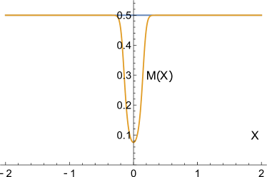
Figure 1: Schematic mass-bump for $X_{4}$-extension.

In addition, in the limit $\varepsilon\to 0$ for the mass-bump case we have the Hamiltonian:

$$L_{X_{4}}^{\varepsilon}=-\frac{1}{2}D_{x}\frac{1}{m_{X_{4}}}D_{x}$$ (11)

with inverse mass operator:

$$\frac{1}{m_{X_{4}}}=\lim\limits_{\varepsilon\to 0}\,\frac{1}{m^{\varepsilon}_{X_{4}}}=2\left(1+X_{4}\,\delta\right)\,.$$ (12)

The Hamiltonian (11) corresponds to the following self-adjoint boundary conditions for (1):

$$M_{X_{4}}=\left(\begin{array}[]{cc}1&-X_{4}\\ 0&1\end{array}\right)\,,$$ (15)

where $X_{4}$ is defined as:

$$X_{4}=\lim\limits_{\varepsilon\to 0}\int\limits_{-\infty}^{\infty}\left(\frac{1}{2\,m_{X_{4}}^{\varepsilon}(x)}-1\right)\,dx\,.$$ (16)

Naturally, the limiting case $m_{X_{4}}^{\varepsilon}(x)\to 1/2$ corresponds to $X_{4}=0$.

In [14] it was shown that by the coordinate transformation $x\to\eta$ the effective-mass Hamiltonian (8) can be transformed into common form of a sum of “kinetic“ and “potential“ terms:

$$\hat{H}_{\alpha}=\frac{1}{2}\,\hat{p}_{\eta}^{2}+\hat{V}_{\alpha}(\eta)\,,$$ (17)

where

$$\hat{V}_{\alpha}(\eta)=\frac{1}{32}(1+4\,\alpha)\left[(1-4\,\alpha)\frac{1}{m}\left(\frac{1}{m}\right)^{\prime}+4\,\left(\frac{1}{m}\right)^{\prime\prime}\right]_{\eta}$$

is the effective potential.

Thus the Hamiltonian (8) in the case $\alpha=0$ and with the position-dependent mass in the form (10) can be represented in standard form:

$$\hat{H}_{X_{4}}^{\varepsilon}=\frac{1}{2}\,\hat{p}^{2}+\frac{X_{4}}{8}\left[2V^{\varepsilon}\,{}^{\prime\prime}+(X_{4}V^{\varepsilon}\,+1)V^{\varepsilon}\,{}^{\prime}\right]_{\eta}\,.$$ (18)

This confirms the results of symmetry analysis of [13] that the mass-bump case ($X_{4}$-extension) belongs to the same class of “potential“ interactions as the standard $\delta$-potential ($X_{1}$-extension).

Note that Hamiltonians (5) and (17) have the same structure if we set $\alpha=1/4$ and $X_{4}=0$, respectively. Thus, the Hamiltonian for extension $X_{2}$ can be written as:

$$L_{X_{2}}^{\varepsilon}=-D_{x}^{2}+\frac{1}{2}\left(\frac{1}{m^{\varepsilon}_{X_{2}}(x)}-\frac{1}{m^{\varepsilon}_{X_{2}}(0)}\right)^{(2)}\,,$$ (19)

where

$$\frac{1}{m^{\varepsilon}_{X_{2}}(x)}=\frac{1}{m^{\varepsilon}_{X_{2}}(0)}+2\,X_{2}\,\int\limits_{0}^{x}V^{\varepsilon}(y)\,dy$$ (20)

so that mass profile has the form of the mass-jump (see Figure 2).

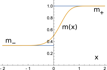
Figure 2: Schematic effective-mass profile of mass-jump for $X_{2}$-extension.

Now we are able to relate the mathematical parameter $X_{2}$ with the mass-jump value. According to [14], the boundary conditions for the singular mass-jump are as follows:

$$\left(\begin{array}[]{c}\psi(0+0)\\ \psi^{\prime}(0+0)\end{array}\right)=\mathcal{T}\,\left(\begin{array}[]{c}\psi(0-0)\\ \psi^{\prime}(0-0)\end{array}\right)\,,\quad\mathcal{T}=\left(\begin{array}[]{cc}\mu^{1/4}&0\\ 0&\frac{1}{\mu^{5/4}}\end{array}\right)\,,$$ (21)

where $\mu=\frac{m_{-}}{m_{+}}$.

In order to compare (21) with that of Kurasov’s boundary conditions (4) we should take into account the appropriate scaling because $X_{2}$-case corresponds to the dilatation symmetry breaking [13, 19] and therefore the appropriate scale choice on the semiaxes is needed for Kurasov’s Hamiltonian. In accordance with the scaling property $x\to\lambda\,x$ for $x>0$, where $\lambda=\mu^{1/2}$. As $\psi_{0+0}\to\lambda^{-1/2}\,\psi_{0+0}\,,\,\,\psi^{\prime}_{0+0}\to\lambda^{-3/2}\,\psi^{\prime}_{0+0}$ then (21) transforms into:

$$\left(\begin{array}[]{c}\psi(0+0)\\ \psi^{\prime}(0+0)\end{array}\right)=\left(\begin{array}[]{cc}\sqrt{\mu}&0\\ 0&\frac{1}{\sqrt{\mu}}\end{array}\right)\,\left(\begin{array}[]{c}\psi(0-0)\\ \psi^{\prime}(0-0)\end{array}\right)\,.$$ (22)

Comparing Kurasov’s boundary conditions (4) with (22) we obtain the following relation between $\mu$ and $X_{2}$:

$$X_{2}=\pm 2\,\frac{\sqrt{\mu}-1}{\sqrt{\mu}+1}\,.$$ (23)

Naturally, the limiting case $\mu\to 1$ leads to $X_{2}=0$ and if $\mu\to 0$ or $\mu\to\infty$ then $|X_{2}|\to 2$. Here we do not use of the results of work [9] where this $X_{2}$-case was coupled with $X_{1}$ interaction. Also we note that from (23) $X_{2}<2$ and the case $X_{2}>2$ differs only by additional $\pi$-phase. This is indirect hint on he magnetic nature of this singular interaction and we prove it in Section 2.

As an example possible application of such point interaction one can consider the energy filter consisting of two such defects (see Figure 3). Such filter demonstrates high energetic selectivity as the analysis of transmission coefficient shows (see Figure 4).

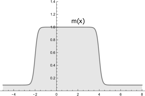
Figure 3: Mass profile for $X_{2}$-filter.

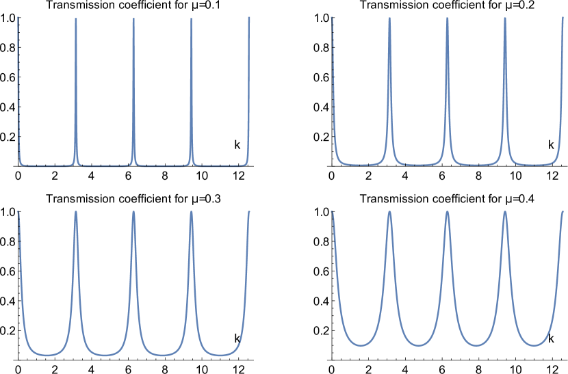
Figure 4: Transmission coefficient of $X_{2}$-filter.

Despite the fact that $X_{2}$ point interaction can be described by the Hamiltonian with the position-dependent effective mass in the following section we demonstrate that it also contains a quantized magnetic flux.

2 Localized quantum magnetic field in $X_{2}$-extension

According to symmetry considerations [13] $X_{2}$-case includes non-zeroth localized quantized magnetic flux. From the symmetry point of view $X_{2}$-extension rather belongs to the same “magnetic“ branch as the $X_{3}$-extension associated with the following boundary conditions of localized magnetic flux $\gamma=\frac{\Phi}{2\,\pi}$ which is related to Kurasov’s Hamiltonian parameter $X_{3}$ as following:

$$\rme^{\rmi\,2\,\pi\gamma}=\frac{2+\rmi\,X_{3}}{2-\rmi\,X_{3}}\,.$$ (24)

The magnetic nature of $X_{3}$-extension is obvious and manifest itself also in scattering matrix:

$$\hat{S}_{X_{3}}=\left(\begin{array}[]{cc}0&\rme^{\rmi\,2\,\pi\gamma}\\ \rme^{-\rmi\,2\,\pi\gamma}&0\end{array}\right)\,,$$ (27)

so that $S^{T}\neq S$ which means the time reversal symmetry breaking because of the magnetic field. Sure if $\gamma=n,\,n\in\mathbb{Z}$ we have “hidden“ non-zeroth flux. This is exactly what happens in $X_{2}$-extension and we show it below.

The magnetic nature of $X_{2}$-extension can be demonstrated by considering it on a circle $S^{1}$. In such geometry the momentum transforms into angular one and becomes quantized with the magnetic quantum number $\mathfrak{m}$. As is known non-magnetic interactions do not break the degeneration of the energy levels $E_{\mathfrak{m}}=E_{-\mathfrak{m}}$ only magnetic ones do it. Standard solution of the boundary problem on a circle (interval $[-1,1]$ with its ends glued and the singular interaction located at $x=0$) shows that $X_{2,3}$-extensions has identical spectra. For $X_{3}$-extension the spectrum is given by the equation:

$$\cos{2\pi\,\gamma}=\cos{2\,k}\,,\quad E=k^{2}$$ (28)

and for $X_{2}$-extension it is:

$$\cos{2\,k}=\frac{2\,\sqrt{\mu}}{1+\mu}\,,\quad E=k^{2}\,.$$ (29)

Obviously (28) and (29) coincide up to the reparametrization:

$$\cos{2\pi\,\gamma}=\frac{2\,\sqrt{\mu}}{1+\mu}\,,\quad\mu>0,\,\,|\gamma|\leq 1/4$$ (30)

which gives the relation between the extension parameters $X_{2}$ and $X_{3}$ in the appropriate region of parameters $\mu$ and $\gamma$. But now the states with $m$ and $-m$ are non-degenerate since the states $\left|\,{\mathfrak{m}+\gamma}\,\right\rangle$ and $\left|\,{-\mathfrak{m}+\gamma}\,\right\rangle$ have different energies $E_{\pm\mathfrak{m}}(\gamma)=(\gamma\pm\mathfrak{m})^{2}$, i.e. the splitting due to the magnetic field is $\Delta E=4\,|\mathfrak{m}|\,\gamma$ (see Figure 5). This proves the existence of magnetic field in these cases. The peculiarity of $X_{2}$-extension is that the “magnetic“ splitting is caused by the integer magnetic flux but its magnitude is govern by the electrostatic $\mu$-interaction which is attributed to the singular effective-mass profile. The parameter $\mu$ itself is non magnetic in nature by its symmetry though it determines the energetic width of splitting because of the presence of the integer point-like magnetic flux which is unobservable by itself because the boundary conditions matrix $M$ as well as scattering matrix becomes trivial (unit matrix) in such a case.

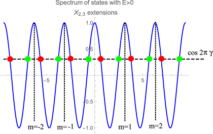
Figure 5: Spectrum of states with $E>0$ on a circle for $X_{2},X_{3}$-extensions. The states of the branch with $\gamma>0$ are colored by red, the ones for $\gamma<0$ branch are green

Also note that in case $X_{2}>2$ additional $\pi$-phase appears although from (23) it follows that $X_{2}<2$. We treat this as another evidence of the quantized magnetic flux so both integer and half-integer quantized flux are described by singular $X_{2}$ interaction.

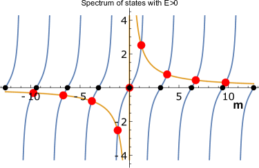
Figure 6: Spectrum of states with $E>0$ on a circle for $X_{1}$-extension. Black points are standard states, the red ones are emergent due to $X_{1}$-defect.

Now we demonstrate that there is no magnetic splitting for $X_{1,4}$ point interactions on circle. Though the spectra of $X_{1}$ and $X_{4}$ are different the degeneracy of the energy levels for states $\left|\,{\pm\mathfrak{m}}\,\right\rangle$ remains. Indeed, they shift symmetrically with respect to the state with $\left|\,{m=0}\,\right\rangle$ (see Figures 6, 7).

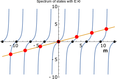
Figure 7: Spectrum of states with $E>0$ on a circle for $X_{4}$-extension. Black points are standard states, the red ones are emergent due to $X_{4}$-defect.

Namely, the spectrum of states $E=k^{2}>0$ for $X_{1}$-extension is:

$$\sin{k}\,\left(X_{1}\,\cos{k}-2\,k\,\sin{k}\right)=0\,\,\Rightarrow\,\,k^{(0)}_{\mathfrak{m}}=\pi\,\mathfrak{m}k^{(1)}\,\tan{k^{(1)}}=X_{1}/2$$ (31)

and the one of $X_{4}$-extension is:

$$\sin{k}\,\left(X_{4}\,k\,\cos{k}-2\,\sin{k}\right)=0\quad\Rightarrow\quad k^{(0)}_{\mathfrak{m}}=\pi\,\mathfrak{m}\,,\quad\tan{k^{(1)}}=X_{4}\,k^{(1)}/2\,.$$ (32)

Thus we have demonstrated the physical nature of point-like interactions and established the magnetic nature of the point interaction for $X_{2}$-extension.

Conclusion

The paper contains two main results. The first one is that non-standard singular self-adjoint extensions $X_{2}$, $X_{4}$ can be described by the position-dependent effective-mass Hamiltonian. The first case can be realized as the “mass-bump“ (see Figure 1). The second one corresponds to the “mass-jump“(see Figure 2) with explicit breaking of the dilatation symmetry $x\to\lambda\,x$ [19]. In addition, we state that despite this similarity these extensions differ with respect to the time reversal symmetry. A quantized magnetic flux is present in $X_{2}$-extension, while $X_{4}$-extension is of pure potential, i.e. “electrostatic“ nature. Thus, according to the classification of [13], we have two extensions $X_{1}$, $X_{4}$ of the potential nature and two extensions $X_{2}$, $X_{3}$ where there is a magnetic field. Possible physical realization of $X_{2}$-extension can be related with the Josephson junctions and other quasi-one-dimensional heterogeneous structures, where the quantized magnetic flux is localized in the transition layer.

References

References

- [1] Berezin F and Faddeev L 1961 Soviet Math. Doklady 2 372–375
- [2] Demkov Yu and Ostrovsky V 1988 Zero-range Potentials and their Applications in Atomic Physics (Plenum, New York)
- [3] Albeverio S, Gesztesy F, Høegh-Krohn R and Holden H 2005 Solvable Models in Quantum Mechanics 2nd ed vol 350 (AMS Chelsea Publishing, Providence, RI, USA)
- [4] Adamyan V 1992 Operator Theory: Advances and Applications 59 1–10
- [5] Tishchenko S 2006 Low Temperature Physics 32 953–956
- [6] Adamyan V and Tishchenko S 2007 Journal of Physics: Condensed Matter 19 186206
- [7] Gallup G 1991 Chem. Phys. Lett. 187 187–192
- [8] Gadella M, Kuru S and Negro J 2007 Physics Letters A 362 265–268
- [9] Gadella M, Heras F, Negro J and Nieto L 2009 Journal of Physics A: Mathematical and Theoretical 42 465207
- [10] Kurasov P 1996 Journal of Mathematical Analysis and Applications 201 297–323
- [11] Kurasov P and Boman J 1998 Proceedings of the American Mathematic Society 126 1673–1683
- [12] Albeverio S and Kurasov P 2000 Singular Perturbations of Differential Operators. Solvable Schrödinger Type Operators (London Mathematical Society Lecture Note Series vol 271) (Cambridge University Press, Cambridge, UK)
- [13] Kulinskii V and Panchenko D 2015 Physica B: Condensed Matter 472 78–83
- [14] Balian R, Bessis D and Mezincescu G 1995 Phys. Rev. B 51(24) 17624–17629
- [15] Roos O 1983 Phys. Rev. B 27(12) 7547–7552
- [16] Morrow R and Brownstein K 1984 Phys. Rev. B 30(2) 678–680
- [17] Morrow R 1987 Phys. Rev. B 35(15) 8074–8079
- [18] Einevoll G and Hemmer P 1988 Journal of Physics C: Solid State Physics 21 L1193
- [19] Albeverio S, Dabrowski L and Kurasov P 1998 Letters in Mathematical Physics 45 33–47