Speeding up complex multivariate data analysis in Borexino with parallel computing based on Graphics Processing Unit

Abstract

A spectral fitter based on the graphics processor unit (GPU) has been developed for Borexino solar neutrino analysis. It is able to shorten the fitting time to a superior level compared to the CPU fitting procedure. In Borexino solar neutrino spectral analysis, fitting usually requires around one hour to converge since it includes time-consuming convolutions in order to account for the detector response and pile-up effects. Moreover, the convergence time increases to more than two days when including extra computations for the discrimination of ¹¹C and external $\gamma$s. In sharp contrast, with the GPU-based fitter it takes less than 10 seconds and less than four minutes, respectively. This fitter is developed utilizing the GooFit project with customized likelihoods, pdfs and infrastructures supporting certain analysis methods. In this proceeding the design of the package, developed features and the comparison with the original CPU fitter are presented.

1 Introduction

The complexity of the analysis techniques increased rapidly in the past 50 years thanks to the Moore’s law on the computation power. Besides the improvement of the single chip computation power, recently the development of the numerous-cores chip and parallel programming toolkit can speed up the analysis even more and the parallel computing becomes more and more popular.

Borexino is a liquid scintillator based neutrino experiment located in Laboratori Nazionali del Gran Sasso in Italy. In Borexino analysis, one of the methods uses the analytical function to model the detector response. Many analysis technologies, such as the multivariate analysis, are used to suppress backgrounds. As a result, the computation becomes too heavy and specific efforts are needed to reduce the fitting time, so we have developed a package to speed up the analysis utilizing the parallel computing techniques working on the Graphic Processing Unit (GPU). The expected number of events in each bin are computed simultaneously by thousands of core in the GPU. It is found to be able to speed up the fitting by more than 2000 times compared with the original code, and thus becomes widely used in analyses[1, 2]. In this proceeding we briefly introduced the package[3] and presented its performance.

2 The Borexino experiment

The Borexino detector is a liquid scintillator based calorimeter. Its structure is shown schematically in Figure 1[4]. In the most inner part there is the target, an organic solution. Its solvent is PC (pseudocumene, 1,2,4-trimethylbenzene C₆H₃(CH₃)₃), and the solute is PPO (2,5-diphenyloxazole, C₁₅H₁₁NO) at a concentration of 1.5 g/L (0.17% by weight). Its mass is around 278 tons. The neutrinos can be detected via the elastic scattering channel on electrons, and the anti-neutrinos can be detected via the inverse beta decay on the hydrogen atoms. Separated by the inner vessel (IV), a 125 $\mu$m specially treated ultra-low-radioactivity nylon vessel, it was surrounded by quenched liquid scintillator which shields it from the gammas rays from the natural radioactivity in the PMTs and stainless steel sphere (SSS). Another nylon vessel, the outer vessel, together with the inner vessel works both as the barriers against radon atoms diffusing inward from outer part of the detector. The radius of the inner vessel, outer vessel and the stainless steel sphere are 4.25 m, 5.5 m and 6 m, respectively. Outside the stainless steel sphere there is the water Cherenkov detector as the active muon veto. 3800 meters water equivalent rock provides passive shield to further suppress muon and cosmogenic backgrounds.

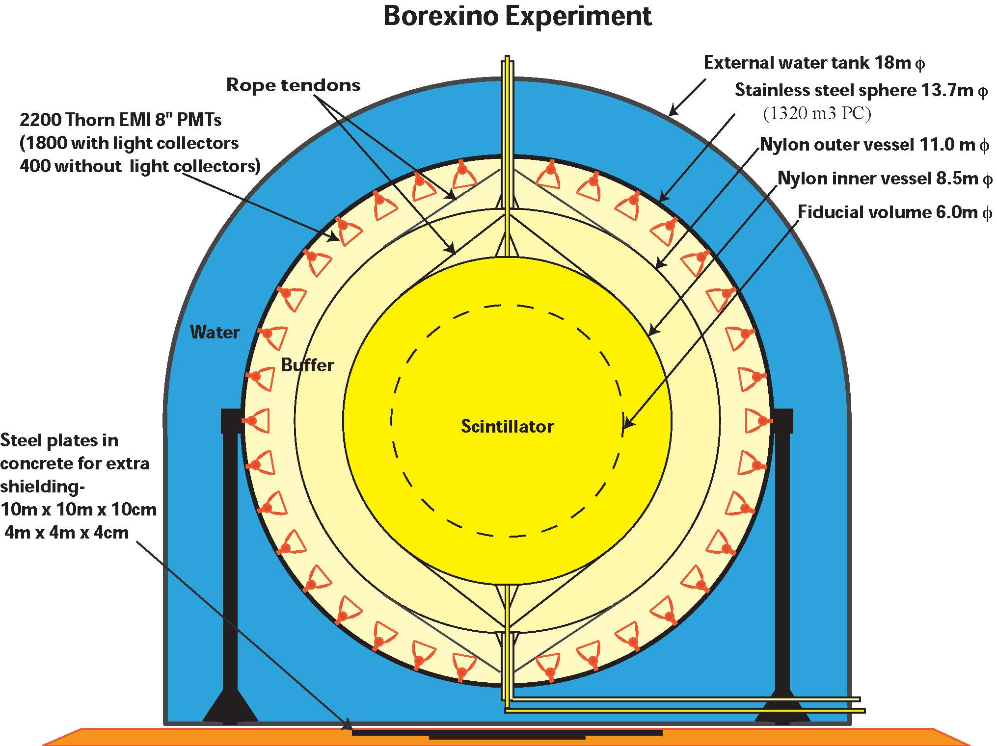
Figure 1: Schematic drawing of Borexino detector.

The scintillation light is collected by 2212 PMTs installed on the inner surface of the stainless steel sphere. The number of photonelectrons collected by Borexino detector is around 500 p.e./MeV/2000 PMTs and the region of interests extends from tens of keV up to a few MeV, so PMTs work in single p.e. regime mostly. The multiple hit probability is of the order of 10% for a 1 MeV energy deposition event in the detector center. For each hit, two signals, one for the energy and one for the time measurements, are produced by the front-end circuit[5]. The energy signal is produced by a special analogues gateless charge integrator. The integrator automatically resets itself and has no dead time. By sampling the integrator output twice separated by 80 ns the charge due to the p.e. arriving during this period is obtained. The timing signal is produced by amplifying the PMT signal with two low noise amplifiers.

Since the start of data taking on May 2007, Borexino has given the current best measurement of ⁷Be solar neutrinos[6], the first evidence of pep solar neutrinos and the best upper limit on solar CNO neutrino flux[7], the only real time detection of pp solar neutrinos[Mosteiro2015b], as well as the ⁸B solar neutrinos with the lowest threshold as low as 3 MeV[8, 9]. Borexino also gave the detection of geo-neutrinos [10] and provided various rare processes studies. Additionaly, it is planned to search for sterile neutrino using an artificial ¹⁴⁴Ce-¹⁴⁴Pr source via short baseline neutrino oscillation within the SOX project[10].

3 Complexity in the Borexino analysis

In Borexino analysis, there are three energy estimators. For each estimator, both two methods, the analytical method and the Monte Carlo method, are studied extensively to describe the actual status of the detector honestly.

In the analytical method, the deposited energy spectrum is calculated priorly, then the visible energy spectrum is predicted by convolving the deposited energy spectrum with the response function

$$f_{\text{vis}}(N_{x})=\int f_{\text{deposit}}(E)\cdot R_{x}(N_{x},E;p_{0},p_{1},...)\;\text{d}E$$ (1)

where $N_{x}$ is the variable used in the analysis, such as the charge, number of detected photons, number of fired channels etc., $f_{\text{vis}}(N_{x})$ is the visible energy spectrum, i.e. the spectrum of variable $N_{x}$, $f_{\text{deposit}}(E)$ is the spectrum of the deposited energy, $R_{x}$ is the corresponding response function, $p_{0},\,p_{1},...$ are its parameters[11].

To have unbiased results with analytical response function, several techniques are developed. The pile-up events are the critical background for $\nu$(pp) signal. To get precise $\nu$(pp) rate, we modelled the pile-up effect by convolving the visible energy spectrum with the spectrum acquired with random trigger.

$$f_{\text{w/ pile-up}}(N_{x0})=\int f_{\text{w/o pile-up}}(N_{x})\cdot g_{\text{random trigger}}(N_{x0}-N_{x})\;\text{d}N_{x}$$ (2)

where $g_{\text{random trigger}}$ is the spectrum of $N_{x}$ variable from random trigger.

To improve the sensitivity on $\nu$(pep) the three-fold-coincidence techniques is used to suppress the cosmogenic ¹¹C. The techniques tags events associated with a muon event and a subsequent neutron event. Since $\nu$(⁷Be) and $\nu$(pp) neutrino are not affected by the ¹¹C, instead of applying cuts we fit both spectra with a joint likelihood to increase the exposure for them

$$\mathcal{L}=\mathcal{L}^{\text{TFC vetoed}}+\mathcal{L}^{\text{TFC tagged}}$$ (3)

To further suppress the impact of the backgrounds for $\nu$(pep), multivariate analysis is developed. We include the radius in the likelihood to suppress the $\gamma$s from the natural radioactivity from PMTs etc. and include the pulse shape parameter to suppress the residual cosmogenic ¹¹C after TFC-veto. Instead of a real high-dimensional fit, the radial and pulse-shape information are included by adding additional terms of likelihood[12].

$$\mathcal{L}^{\text{multivariaite}}=\mathcal{L}^{\text{TFC vetoed}}+\mathcal{L}^{\text{TFC tagged}}+\sum_{i}\mathcal{L}^{\text{radial}}_{i}+\sum_{j}\mathcal{L}^{\text{pulse-shape}}_{j}$$ (4)

The analytical response function is validated against Monte Carlo p.d.f. Toy Monte Carlo spectra are prepared and are fitted against the analytical response function. The fit results are not biased, so the analytical response function is able to describe the detector response, at least as good as the Monte Carlo p.d.f.

4 GPU based parallel computing

To speed up the computation, a new fitting tool based on GPU is developed. Because the computations of the expected number of events in each bin are independent, they can be performed simultaneously by thousands of cores inside the GPU and thus the fitting time is reduced significantly. An existing project GooFit is used as the interface between the minimization package and the GPU. TMinuit from ROOT is used as the minimization engine.

The workflow of package, controlled by the AnalysisManager object, is the following:

1. Load the fit configuration, the energy histogram and miscellaneous information such as the exposure etc. into the InputDataManager;

2. Construct the energy spectrum, the response function object, the dataset and all likelihood terms;

3. Construct the TMinuit object;

4. The GooFit associate the constructed likelihood object to the the TMinuit object;

5. Call the TMinuit::minimize method. The TMinuit will vary the parameters and evaluate the likelihood and find the maximum of the likelihood;

6. When TMinuit requests the evaluation of the likelihood, the control is passed to GooFit, GooFit will launch the parallel computation and evaluate the expected number of events in each bin simultaneously. The evaluation is done by calling the function pointer saved in each likelihood object, and these functions are written in cuda, a C-like advanced programming language for instructing the GPU card;

7. When the TMinuit finds the minimum, the control is given back to package. The fit result is saved and the plots are created.

5 Comparison and validation against the original CPU code

An example output of the package is shown in the left panel of Figure 2. The package is validated against the original CPU version of the fitter. Fits are performed with two fitters under same configuration on the same dataset. The comparison is shown in Figure 2.

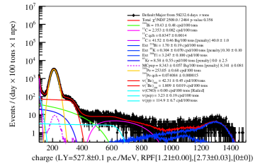
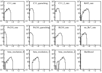
Figure 2: Left panel: An example output with Monte Carlo dataset. Right panel: Comparison between the package and the original fitter. On the $x$-axis it is $\log_{10}|\Delta|$ where $\Delta$ is the difference.

The converging time tested is listed in Table 1. As one can see the speed up is at a factor of more than 2000 when switching on the multivariate likelihood.

Table 1: Comparison between CPU fitter and package.

Type	hardware	no multivaraite	with multivariate
CPU (original package)	AMD Opteron(tm) 6320	$\sim$1 hour	$\sim$5 seconds
GPU (this package)	nVidia K40	$>$1 week	$\sim$4 minutes

6 Outlook

All the analysis techniques used in the solar spectral analysis have been implemented in this package. The package is also validated and has shown an excellent performance. In the near future we plan to implement the multi-dimensional fitting and more sophisticated and accurate response function proposed recently. With a deeper understanding of the principle of GPU and the low level manipulation of the cuda it is foreseen that the performance of the package can be further improved, and an upgrade of the package is planned in the near future.

The Borexino program is made possible by funding from INFN (Italy), NSF (USA), BMBF, DFG, HGF, and MPG (Germany), RFBR (Grants 16-02-01026 A, 15-02-02117 A, 16-29-13014 ofim, 17-02-00305 A) (Russia), and NCN (Grant No. UMO 2013/10/E/ST2/00180) (Poland).

X.F. Ding thanks Marcin Misiaszek, Andrea Meschini and Le Li for providing the GPU resources, Eugenio Coccia, Francesco Vissani, and the GSSI for the support which made this conference contribution possible.

References

References

- [1] Agostini M, Altenmuller K, Appel S et al. 2017 1–8 (Preprint 1707.09279)
- [2] Agostini M, Altenmüller K, Appel S et al. 2017 Physical Review D 96 091103 ISSN 2470-0010 (Preprint 1707.09355)
- [3] Ding X 2018 GooStats, a multivariate spectrum fitting analysis package for particle physics accelerated by graphic processing units URL https://doi.org/10.5281/zenodo.1217007
- [4] Alimonti G, Arpesella C, Back H et al. 2009 Nuclear Instruments and Methods in Physics Research, Section A: Accelerators, Spectrometers, Detectors and Associated Equipment 600 568–593 ISSN 01689002 (Preprint 0806.2400)
- [5] Lagomarsino V and Testera G 1999 Nuclear Instruments and Methods in Physics Research Section A: Accelerators, Spectrometers, Detectors and Associated Equipment 430 435–446 ISSN 01689002
- [6] Bellini G, Benziger J, Bick D et al. 2011 Physical Review Letters 107 1–5 ISSN 00319007 (Preprint 1104.2150)
- [7] Bellini G, Benziger J, Bick D et al. 2012 Physical Review Letters 108 1–6 ISSN 00319007 (Preprint 1110.3230)
- [8] Bellini G, Benziger J, Bonetti S et al. 2010 Physical Review D 82 033006 ISSN 1550-7998 (Preprint 0808.2868)
- [9] The Borexino Collaboration, Agostini M, Altenmueller K et al. 2017 016 1–13 (Preprint 1709.00756)
- [10] Bellini G, Bick D, Bonfini G et al. 2013 Journal of High Energy Physics 2013 38 ISSN 1029-8479 (Preprint 1304.7721)
- [11] Bellini G, Benziger J, Bick D et al. 2014 Physical Review D - Particles, Fields, Gravitation and Cosmology 89 1–68 ISSN 15502368 (Preprint 1308.0443)
- [12] Davini S 2013 The European Physical Journal Plus 128 89 ISSN 2190-5444