Common Origin of Dirac Neutrino Mass and
Freeze-in Massive Particle Dark Matter

Abstract

Motivated by the fact that the origin of tiny Dirac neutrino masses via the standard model Higgs field and non-thermal dark matter populating the Universe via freeze-in mechanism require tiny dimensionless couplings of similar order of magnitudes $(\sim 10^{-12})$, we propose a framework that can dynamically generate such couplings in a unified manner. Adopting a flavour symmetric approach based on $A_{4}$ group, we construct a model where Dirac neutrino coupling to the standard model Higgs and dark matter coupling to its mother particle occur at dimension six level involving the same flavon fields, thereby generating the effective Yukawa coupling of same order of magnitudes. The mother particle for dark matter, a complex scalar singlet, gets thermally produced in the early Universe through Higgs portal couplings followed by its thermal freeze-out and then decay into the dark matter candidates giving rise to the freeze-in dark matter scenario. Some parts of the Higgs portal couplings of the mother particle can also be excluded by collider constraints on invisible decay rate of the standard model like Higgs boson. We show that the correct neutrino oscillation data can be successfully produced in the model which predicts normal hierarchical neutrino mass. The model also predicts the atmospheric angle to be in the lower octant if the Dirac CP phase lies close to the presently preferred maximal value.

I Introduction

Although the non-zero neutrino mass and large leptonic mixing are well established facts by now Patrignani et al. (2016), with the present status of different neutrino parameters being shown in global fit analysis Esteban et al. (2017); de Salas et al. (2017), we still do not know a few things about neutrinos. They are namely, (a) nature of neutrinos: Dirac or Majorana, (b) mass hierarchy of neutrinos: normal $(m_{3}>m_{2}>m_{1})$ or inverted $(m_{2}>m_{1}>m_{3})$ and (c) leptonic CP violation as well as the octant of atmospheric mixing angle $\theta_{23}$. While neutrino oscillation experiments are not sensitive to the nature of neutrinos, experiments looking for lepton number violating signatures like neutrinoless double beta decay $(0\nu\beta\beta)$ have the potential to confirm the Majorana nature of neutrinos with a positive signal. Although the oscillation experiments are insensitive to the lightest neutrino mass, the negative results at $(0\nu\beta\beta)$ experiments have been able to disfavour the quasi-degenerate regime of light neutrino masses. Similarly, the cosmology experiment Planck has also constrained the lightest neutrino mass from its bound on the sum of absolute neutrino masses $\sum m_{i}\leq 0.17$ eV Ade et al. (2016).

On the other hand, in cosmic frontier, we have significant amount of evidences Zwicky (1933); Rubin and Ford (1970); Clowe et al. (2006); Hinshaw et al. (2013); Ade et al. (2016) suggesting the presence of non-baryonic form of matter, or the so called Dark Matter (DM) in large amount in the present Universe. According to the latest cosmology experiment Planck Ade et al. (2016), almost $26\%$ of the present Universe’s energy density is in the form of DM while only around $5\%$ is the usual baryonic matter leading the rest of the energy budget to mysterious dark energy. Quantitatively, the DM abundance at present is quoted as $0.1172\leq\Omega_{\rm DM}h^{2}\leq 0.1226$ at 67% C.L. Ade et al. (2016) where $\Omega_{\rm DM}=\rho_{\rm DM}/\rho_{\rm cr}$ is the DM density parameter with $\rho_{\rm cr}=\frac{3H^{2}_{0}}{8\pi G}$ being the critical density of the Universe and $H_{0}$ being the present value of the Hubble parameter. The dimensionless parameter $h$ is $H_{0}/100$. In spite of all these evidences, we do not yet know the particle nature of DM.

Since the standard model (SM) of particle physics fails to address the problem of neutrino mass and dark matter, several beyond standard model (BSM) proposals have been put forward in order to accommodate them. While seesaw mechanism Minkowski (1977); Gell-Mann et al. (1979); Mohapatra and Senjanovic (1980); Schechter and Valle (1980) remains the most popular scenario for generating tiny neutrino masses, the weakly interacting massive particle (WIMP) paradigm has been the most widely studied dark matter scenario. In this framework, a dark matter candidate typically with electroweak scale mass and interaction rate similar to electroweak interactions can give rise to the correct dark matter relic abundance, a remarkable coincidence often referred to as the WIMP Miracle. Now, if such type of particles whose interactions are of the order of electroweak interactions really exist then we should expect their signatures in various DM direct detection experiments where the recoil energies of detector nuclei scattered by DM particles are being measured. However, after decades of running, direct detection experiments are yet to observe any DM-nucleon scattering Tan et al. (2016); Aprile et al. (2017); Akerib et al. (2017). The absence of dark matter signals from the direct detection experiments have progressively lowered the exclusion curve in its mass-cross section plane. Although such null results could indicate a very constrained region of WIMP parameter space, they have also motivated the particle physics community to look for beyond the thermal WIMP paradigm where the interaction scale of DM particle can be much lower than the scale of weak interaction i.e.  DM may be more feebly interacting than the thermal WIMP paradigm. One of the viable alternatives of WIMP paradigm, which may be a possible reason of null results at various direct detection experiments, is to consider the non-thermal origin of DM Hall et al. (2010). In this scenario, the initial number density of DM in the early Universe is negligible and it is assumed that the interaction strength of DM with other particles in the thermal bath is so feeble that it never reaches thermal equilibrium at any epoch in the early Universe. In this set up, DM is mainly produced from the out of equilibrium decays of some heavy particles in the plasma. It can also be produced from the scatterings of bath particles, however if same couplings are involved in both decay as well as scattering processes then the former has the dominant contribution to DM relic density over the latter one Hall et al. (2010); Biswas and Gupta (2016); Biswas et al. (2017). The production mechanism for non-thermal DM is known as freeze-in and the candidates of non-thermal DM produced via freeze-in are often classified into a group called Freeze-in (Feebly interacting) massive particle (FIMP). For a recent review of this DM paradigm, please see Bernal et al. (2017). Similarly, the popular seesaw models predict Majorana nature of neutrinos though the results from $0\nu\beta\beta$ experiments have so far been negative. Although such negative results do not necessarily prove that the light neutrinos are of Dirac nature, it is nevertheless suggestive enough to come up with scenarios predicting Dirac neutrinos with correct mass and mixing. This has led to several proposals that attempt to generate tiny neutrino masses in a variety of ways Babu and He (1989); Peltoniemi et al. (1993); Centelles Chuliá et al. (2017a); Aranda et al. (2014); Chen et al. (2016); Ma et al. (2015); Reig et al. (2016); Wang and Han (2016); Wang et al. (2017, 2006); Gabriel and Nandi (2007); Davidson and Logan (2009, 2010); Bonilla and Valle (2016); Farzan and Ma (2012); Bonilla et al. (2016); Ma and Popov (2017); Ma and Sarkar (2018); Borah (2016); Borah and Dasgupta (2016); Borah and Dasgupta (2017a, b); Centelles Chuliá et al. (2017b); Bonilla et al. (2018); Memenga et al. (2013); Borah and Karmakar (2018); Centelles Chuliá et al. (2018a, b); Han and Wang (2018), some of which also accommodate the origin of WIMP type dark matter simultaneously.

The present article is motivated by the coincidence that the origin of Dirac neutrino masses as well as FIMP dark matter typically require very small dimensionless couplings $\sim 10^{-12}$ Hall et al. (2010). In the neutrino sector, such couplings can generate $0.1$ eV Dirac neutrino mass through neutrino coupling to the standard model like Higgs. On the other hand, in the dark sector, such tiny couplings of the dark matter particle with the mother particle makes sure that it gets produced non-thermally through the freeze-in mechanism. There have been several attempts where the origin of such feeble interactions of DM with the visible sector is generated via higher dimensional effective operators Hall et al. (2010); Elahi et al. (2015); McDonald (2016). Very recently, there has been attempt to realise such feeble interactions naturally at renormalisable level also Biswas et al. (2018). The coincidence between such tiny FIMP couplings and Dirac neutrino Yukawas was also pointed out, mostly in supersymmetric contexts, by the authors of Hall et al. (2010); Gopalakrishna et al. (2006); de Gouvea et al. (2006); Page (2007); Asaka et al. (2007, 2006). Here, we consider an $A_{4}$ flavour symmetric model where neutrino Dirac mass as well as FIMP coupling with its mother particle get generated through dimension six operators involving the same flavon fields. A global unbroken lepton number symmetry is assumed that forbids the Majorana mass terms of singlet fermions. We show that both freeze-in and freeze-out formalisms are important in generating the dark matter relic in our scenario. The mother particle, which is long lived in this model and decays only to the dark matter at leading order, first freezes out and then decays into the dark matter particle. Therefore, the final abundance of dark matter particle depends upon the mother particle couplings to the standard model particles which can be probed at different ongoing experiments. Interestingly, we find that ongoing experiments like the large hadron collider (LHC) can probe some part of the parameter space which can give rise to sizeable invisible decay of SM like Higgs boson into the long lived mother particles. We also show that the correct neutrino oscillation data can be reproduced in some specific vacuum alignments of the flavon fields indicating the predictive nature of the model. The model also predicts normal hierarchical neutrino mass ordering and interesting correlations between neutrino parameters requiring the atmospheric mixing angle to be in the lower octant for maximal Dirac CP phase.

The remaining part of this letter is organised as follows. In section II we discuss our $A_{4}$ flavour symmetric models of Dirac neutrino mass and FIMP dark matter and discuss the consequences for neutrino sector for some benchmark scenarios. In section III, we discuss the calculation related to relic abundance of dark matter and then finally conclude in section IV.

II $A_{4}$ Model for Dirac neutrinos and FIMP dark matter

We first consider a minimal model based on $A_{4}$ flavour symmetry that can give rise to tiny Dirac neutrino masses and mixing at dimension six level. A brief details of $A_{4}$ group is given in appendix A. The fermion sector of the standard model is extended by three copies of gauge singlet right handed neutrinos ($\nu_{R}$) and an additional gauge singlet fermion ($\psi$) which plays the role of FIMP dark matter. These right handed neutrinos transform in the same way just like the standard model lepton doublets ($L$) do under $A_{4}$, a typical feature of most of the $A_{4}$ flavour symmetric realisations of neutrino mass. We also introduce four different flavon fields for the desired phenomenology of neutrino mass and dark matter. The $A_{4}$ flavour symmetry is augmented by additional discrete symmetries $Z_{4}\times Z^{\prime}_{4}$ and a global unbroken lepton number symmetry $U(1)_{L}$ in order to forbid the unwanted terms. Transformations of the fields under the complete flavour symmetry of the model $A_{4}\times Z_{4}\times Z^{\prime}_{4}\times U(1)_{L}$ are given in Table 1.

Fields	$L$	$e_{\mbox{\tiny$R$}},\mu_{\mbox{\tiny$R$}},\tau_{\mbox{\tiny$R$}}$	$H$	$\nu_{\mbox{\tiny$R$}}$	$\psi$	$\phi_{S}$	$\phi_{\mbox{\tiny$T$}}$	$\zeta$	$\eta$
$A_{4}$	3	1,$1^{\prime\prime}$,$1^{\prime}$	1	3	1	3	3	1	1
$Z_{4}$	-$i$	-$i$	1	$i$	$i$	$i$	1	$i$	1
$Z^{\prime}_{4}$	1	1	1	1	$i$	1	1	$i$	$-1$
$U(1)_{L}$	1	1	0	1	0	0	0	0	0

Table 1: Field content and transformation properties under $A_{4}\times Z_{4}\times Z^{\prime}_{4}\times U(1)_{L}$ symmetry of the model.

The construction here includes two $A_{4}$ triplet flavons, $\phi_{\mbox{\tiny$T$}}$ and $\phi_{\mbox{\tiny$S$}}$, which play a crucial role in generating masses and mixing for charged leptons and Dirac neutrinos respectively. Now, for charged lepton sector, the relevant Yukawa Lagrangian can be written as

$$\mathcal{L}_{l}=\frac{y_{e}}{\Lambda}(\bar{L}\phi_{\mbox{\tiny$T$}})He_{\mbox{\tiny$R$}}+\frac{y_{\mu}}{\Lambda}(\bar{L}\phi_{\mbox{\tiny$T$}})_{1^{\prime}}H\mu_{\mbox{\tiny$R$}}+\frac{y_{\tau}}{\Lambda}(\bar{L}\phi_{\mbox{\tiny$T$}})_{1^{\prime\prime}}H\tau_{\mbox{\tiny$R$}}$$ (1)

where $\Lambda$ is the cut-off scale of the theory. Here and subsequently all the $y$’s stand for the respective coupling constants, unless otherwise mentioned. The leading contributions to the charged lepton mass via $\bar{L}H\ell_{i}$ (where $\ell_{i}$ are the RH charged leptons) are not allowed due to the specific $A_{4}$ symmetry. When the triplet flavon $\phi_{\mbox{\tiny$T$}}$ is present in the model it leads to an $A_{4}$ invariant dimension five operator as given in equation (1) which subsequently generates the relevant masses after flavons and the SM Higgs field acquire non-zero vacuum expectation value (vev)’s. Using the $A_{4}$ product rules given in appendix A and taking generic triplet flavon vev alignment $\langle\phi_{T}\rangle=(v_{T},v_{T},v_{T})$, we can write down the charged lepton mass matrix as

$$m_{l}=\frac{vv_{\mbox{\tiny$T$}}}{\Lambda}\left(\begin{array}[]{ccc}y_{e}&y_{\mu}&y_{\tau}\\ y_{e}&\omega y_{\mu}&\omega^{2}y_{\tau}\\ y_{e}&\omega^{2}y_{\mu}&\omega y_{\tau}\end{array}\right).$$ (5)

Here $v$ denotes the vev of the SM Higgs doublet $H$ and $\omega=e^{i2\pi/3}$ is the cube root of unity. This mass matrix can be diagonalised by using the magic matrix $U_{\omega}$, given by

$$U_{\omega}=\frac{1}{\sqrt{3}}\left(\begin{array}[]{ccc}1&1&1\\ 1&\omega&\omega^{2}\\ 1&\omega^{2}&\omega\end{array}\right).$$ (9)

Now, as indicated earlier, the complete $A_{4}\times Z_{4}\times Z^{\prime}_{4}$ discrete symmetry plays an instrumental role in generating tiny Dirac neutrino mass and mixing at dimension six level. Any contribution to the neutrino mass (through $\bar{L}\tilde{H}\nu_{R}$) is forbidden up to dimension five level in the present set-up. Since charged lepton masses are generated at dimension five level, it naturally explains the observed hierarchy between charged and neutral lepton masses. Presence of the $A_{4}$ triplet flavon $\phi_{S}$ generates the required dimension six operator for neutrino mass and mixing. The relevant Yukawa Lagrangian for neutrino sector is given by

$$\mathcal{L}_{\nu} = \bar{L}\tilde{H}\nu_{R}\frac{(\phi_{S})^{2}}{\Lambda^{2}}+\text{h.c.}$$

$$= \frac{y_{s}}{\Lambda^{2}}(\bar{L}\tilde{H}\nu_{R})_{S}(\phi_{S}\phi_{S})_{S}+\frac{y_{s^{\prime}}}{\Lambda^{2}}(\bar{L}\tilde{H}\nu_{R})_{S}(\phi_{S}\phi_{S})_{A}+\frac{y_{a}}{\Lambda^{2}}(\bar{L}\tilde{H}\nu_{R})_{A}(\phi_{S}\phi_{S})_{S}$$

$$+ \frac{y_{a^{\prime}}}{\Lambda^{2}}(\bar{L}\tilde{H}\nu_{R})_{A}(\phi_{S}\phi_{S})_{A}+\frac{y_{x_{1}}}{\Lambda^{2}}(\bar{L}\tilde{H}\nu_{R})_{1}(\phi_{S}\phi_{S})_{1}+\frac{y_{x_{2}}}{\Lambda^{2}}(\bar{L}\tilde{H}\nu_{R})_{1^{\prime}}(\phi_{S}\phi_{S})_{1^{\prime\prime}}$$

$$+ \frac{y_{x_{3}}}{\Lambda^{2}}(\bar{L}\tilde{H}\nu_{R})_{1^{\prime\prime}}(\phi_{S}\phi_{S})_{1^{\prime}}+\text{h.c.}.$$ (11)

Here the subscripts $S$ and $A$ stands for symmetric and anti-symmetric parts of $A_{4}$ triplets products (see Appendix A for details) in the $S$ diagonal basis adopted in the analysis and $1,1^{\prime}$ and $1^{\prime\prime}$ stand for three singlets of $A_{4}$. For the most general vev alignment $\langle\phi_{S}\rangle=(v_{S_{1}},v_{S_{2}},v_{S_{3}})$, the effective mass matrix for neutrinos can be written as

$$m_{\nu} = \left(\begin{array}[]{ccc}x_{11}&s_{21}+a_{21}&s_{31}+a_{31}\\ s_{21}-a_{21}&x_{22}&s_{32}+a_{32}\\ s_{31}-a_{31}&s_{32}-a_{32}&x_{33}\end{array}\right)$$ (15)

where the diagonal elements are given by

$$x_{11}= \left[y_{x_{1}}(v_{S_{1}}^{2}+v_{S_{2}}^{2}+v_{S_{3}}^{2})+y_{x_{2}}(v_{S_{1}}^{2}+\omega^{2}v_{S_{2}}^{2}+\omega v_{S_{3}}^{2})+y_{x_{3}}(v_{S_{1}}^{2}+\omega v_{S_{2}}^{2}+\omega^{2}v_{S_{3}}^{2})\right]v/\Lambda^{2},$$ (16)

$$x_{22}= \left[y_{x_{1}}(v_{S_{1}}^{2}+v_{S_{2}}^{2}+v_{S_{3}}^{2})+y_{x_{2}}\omega(v_{S_{1}}^{2}+\omega^{2}v_{S_{2}}^{2}+\omega v_{S_{3}}^{2})+y_{x_{3}}\omega^{2}(v_{S_{1}}^{2}+\omega v_{S_{2}}^{2}+\omega^{2}v_{S_{3}}^{2})\right]v/\Lambda^{2},$$ (17)

$$x_{33}= \left[y_{x_{1}}(v_{S_{1}}^{2}+v_{S_{2}}^{2}+v_{S_{3}}^{2})+y_{x_{2}}\omega^{2}(v_{S_{1}}^{2}+\omega^{2}v_{S_{2}}^{2}+\omega v_{S_{3}}^{2})+y_{x_{3}}\omega(v_{S_{1}}^{2}+\omega v_{S_{2}}^{2}+\omega^{2}v_{S_{3}}^{2})\right]v/\Lambda^{2}.$$ (18)

Now, the symmetric part originated from $A_{4}$ triplet products are given by

$$s_{32}= y_{s}v(v_{S_{2}}v_{S_{3}}+v_{S_{3}}v_{S_{2}})/\Lambda^{2}+y_{s}^{\prime}v(v_{S_{2}}v_{S_{3}}-v_{S_{3}}v_{S_{2}})/\Lambda^{2},$$ (19)

$$s_{31}= y_{s}v(v_{S_{3}}v_{S_{1}}+v_{S_{1}}v_{S_{3}})/\Lambda^{2}+y_{s}^{\prime}v(v_{S_{3}}v_{S_{1}}-v_{S_{1}}v_{S_{3}})/\Lambda^{2},$$ (20)

$$s_{21}= y_{s}v(v_{S_{1}}v_{S_{2}}+v_{S_{2}}v_{S_{1}})/\Lambda^{2}+y_{s}^{\prime}v(v_{S_{1}}v_{S_{2}}-v_{S_{2}}v_{S_{1}})/\Lambda^{2}.$$ (21)

As seen above, when neutrinos are Dirac fermions instead of Majorana, then there is an additional anti-symmetric contribution in the neutrino mass matrix which remains absent in the Majorana case due to symmetric property of the Majorana mass term. This additional contribution can in fact explain nonzero $\theta_{13}$ in a more economical setup Memenga et al. (2013); Borah and Karmakar (2018); Borah et al. (2017) compared to the one for Majorana neutrinos Karmakar and Sil (2015). In the mass matrix given by equation (15) these anti-symmetric contributions are given by

$$a_{32}= y_{a}v(v_{S_{2}}v_{S_{3}}+v_{S_{3}}v_{S_{2}})/\Lambda^{2}+y_{a}^{\prime}v(v_{S_{2}}v_{S_{3}}-v_{S_{3}}v_{S_{2}})/\Lambda^{2},$$ (22)

$$a_{31}= y_{a}v(v_{S_{3}}v_{S_{1}}+v_{S_{1}}v_{S_{3}})/\Lambda^{2}+y_{a}^{\prime}v(v_{S_{3}}v_{S_{1}}-v_{S_{1}}v_{S_{3}})/\Lambda^{2},$$ (23)

$$a_{21}= y_{s}v(v_{S_{1}}v_{S_{2}}+v_{S_{2}}v_{S_{1}})/\Lambda^{2}+y_{a}^{\prime}v(v_{S_{1}}v_{S_{2}}-v_{S_{2}}v_{S_{1}})/\Lambda^{2}.$$ (24)

The most general mass matrix for Dirac neutrinos given in equation (15) can be further simplified depending upon the specific and simpler vev alignments of the triplet flavon $\phi_{S}$. Here we briefly discuss a few such possible alignments analytically and then restrict ourselves to one such scenario for numerical analysis which can explain neutrino masses and mixing in a minimal way. Note that such vev alignments demand a complete analysis of the scalar sector of the model and can be obtained in principle, from the minimisation of the scalar potential He et al. (2006); Branco et al. (2009); Lin (2009); Dorame et al. (2012); Rodejohann and Xu (2016). For simplicity, when we consider the vev alignment of $\phi_{S}$ to be $\langle\phi_{S}\rangle=(v_{S},v_{S},v_{S})$ from equation (16)-(22), we obtain $s_{32}=s_{31}=s_{21}=2y_{s}vv_{S}^{2}/\Lambda^{2}=s$ (say) and $a_{32}=a_{31}=a_{21}=2y_{a}vv_{S}^{2}/\Lambda^{2}=a$ (say). Hence the neutrino mass matrix takes the form

$$m_{\nu} = \left(\begin{array}[]{ccc}x&s+a&s+a\\ s-a&x&s+a\\ s-a&s-a&x\end{array}\right),$$ (28)

where $x_{11}=x_{22}=x_{33}=3y_{x_{1}}vv_{S}^{2}/\Lambda^{2}=x$ (say). For even more simplified scenarios of vev alignments $\langle\phi_{S}\rangle=(v_{S},v_{S},0)$ and $\langle\phi_{S}\rangle=(0,v_{S},v_{S})$ the neutrino mass matrices are given by

$$m_{\nu} = \left(\begin{array}[]{ccc}x_{11}&s+a&0\\ s-a&x_{22}&0\\ 0&0&x_{33}\end{array}\right);~{}~{}~{}~{}m_{\nu}=\left(\begin{array}[]{ccc}x_{11}&0&0\\ 0&x_{22}&s+a\\ 0&s-a&x_{33}\end{array}\right),$$ (35)

respectively, where the elements are defined as $s_{21}=2y_{s}vv_{S}^{2}/\Lambda^{2}=s$ (say), $a_{21}=2y_{a}vv_{S}^{2}/\Lambda^{2}=a$ (say), $x_{11}=(2y_{x_{1}}-y_{x_{2}}\omega-y_{x_{3}}\omega^{2})vv_{S}^{2}/\Lambda^{2}$, $x_{22}=(2y_{x_{1}}-y_{x_{2}}\omega^{2}-y_{x_{3}}\omega)vv_{S}^{2}/\Lambda^{2}$, $x_{33}=(2y_{x_{1}}-y_{x_{2}}-y_{x_{3}})vv_{S}^{2}/\Lambda^{2}$ and $s_{32}=2y_{s}vv_{S}^{2}/\Lambda^{2}=s$ (say), $a_{32}=2y_{a}vv_{S}^{2}/\Lambda^{2}=a$ (say), $x_{11}=(2y_{x_{1}}-y_{x_{2}}-y_{x_{3}})vv_{S}^{2}/\Lambda^{2}$, $x_{22}=(2y_{x_{1}}-y_{x_{2}}\omega-y_{x_{3}}\omega^{2})vv_{S}^{2}/\Lambda^{2}$, $x_{33}=(2y_{x_{1}}-y_{x_{2}}\omega^{2}-y_{x_{3}}\omega)vv_{S}^{2}/\Lambda^{2}$ respectively. As evident from these two neutrino mass matrices given by equation (35), a Hermitian matrix ($m_{\nu}m_{\nu}^{\dagger}$) obtained from these demands a rotation in the 12 and 23 planes respectively. This, however, is not sufficient to to explain observed neutrino mixing along with the contribution ($U_{\omega}$) from the charged lepton sector given in equation (9). Now, a third possibility with vev alignment $\langle\phi_{S}\rangle=(v_{S},0,v_{S})$, yields a compatible neutrino mass matrix, given by,

$$m_{\nu} = \left(\begin{array}[]{ccc}x_{11}&0&s+a\\ 0&x_{22}&0\\ s-a&0&x_{33}\end{array}\right),$$ (39)

where $s_{31}=2y_{s}vv_{S}^{2}/\Lambda^{2}=s$ (say), $a_{31}=2y_{a}vv_{S}^{2}/\Lambda^{2}=a$ (say), $x_{11}=(2y_{x_{1}}-y_{x_{2}}\omega^{2}-y_{x_{3}}\omega)vv_{S}^{2}/\Lambda^{2}$, $x_{22}=(2y_{x_{1}}-y_{x_{2}}-y_{x_{3}})vv_{S}^{2}/\Lambda^{2}$ and $x_{33}=(2y_{x_{1}}-y_{x_{2}}\omega-y_{x_{3}}\omega^{2})vv_{S}^{2}/\Lambda^{2}$. Although parameters present here are in general complex, for the diagonal elements we consider them to be equal that is, $x_{11}=x_{22}=x_{33}=x$ and real without loss of any generality. Now, to diagonalise this mass matrix, let us first define a Hermitian matrix as

$$\mathcal{M} = m_{\nu}m_{\nu}^{\dagger}$$ (43)

$$= \left(\begin{array}[]{ccc}x^{2}+|s+a|^{2}&0&x(s-a)^{*}+x(s+a)\\ o&x^{2}&0\\ x(s-a)+x(s+a)^{*}&0&x^{2}+|s-a|^{2}\end{array}\right).$$

Here the complex terms corresponding to the symmetric and anti-symmetric parts of $A_{4}$ products can be written as $s=|s|^{i\phi_{s}}$ and $a=|a|^{i\phi_{a}}$. These complex phases essentially dictates the CP violation of the theory. Clearly, the structure of $\mathcal{M}$ given in equation (43) indicates rotation in the 13 plane through the relation $U_{13}^{\dagger}\mathcal{M}U_{13}={\rm diag}(m_{1}^{2},m_{2}^{2},m_{3}^{2})$ is sufficient to diagonalise this matrix, where the $U_{13}$ is given by

$$U_{13}=\left(\begin{array}[]{ccc}\cos\theta&0&\sin\theta{e^{-i\psi}}\\ 0&1&0\\ -\sin\theta{e^{i\psi}}&0&\cos\theta\end{array}\right),$$ (47)

 

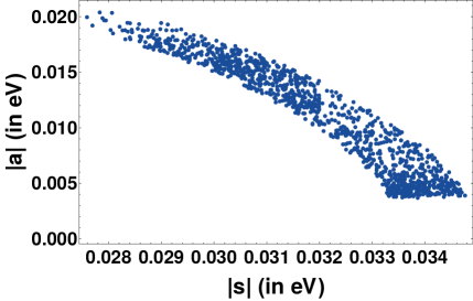
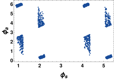
Figure 1: Correlations between different model parameters for 3$\sigma$ allowed ranges of $\theta_{13}$, $\theta_{12}$, $\theta_{23}$, mass squared differences Esteban et al. (2017) and $\sum m_{i}\leq 0.17$ eV. Left panel: the allowed points in $|s|-|a|$ (symmetric and anti-symmetric parts of the neutrino mass matrix respectively) plane. Right panel: the allowed points in the $\phi_{s}-\phi_{a}$ (phases associated with symmetric nd anti-symmetric parts respectively) plane.

and the mass eigenvalues are found to be

$$m_{1}^{2} = x^{2}+A-B,$$ (48)

$$m_{2}^{2} = x^{2},$$ (49)

$$m_{3}^{2} = x^{2}+A+B,$$ (50)

where $A=|s|^{2}+|a|^{2}$ and $B=\sqrt{(2|s||a|\cos(\phi_{s}-\phi_{a}))^{2}+4x^{2}(|s|^{2}\cos^{2}\phi_{s}+|a|^{2}\sin^{2}\phi_{a})}$. One important inference of such ordering is that inverted hierarchy of neutrino mass is not feasible in this setup as $\Delta m^{2}_{23}+\Delta m^{2}_{21}=-2(|s|^{2}+|a|^{2})<0$, implying $m_{3}>m_{2}$. Also, the two parameters $\theta$ and $\psi$ appearing in $U_{13}$ can be expressed as

$$\tan 2\theta=\frac{x(|a|\sin\phi_{a}\sin\psi-|s|\cos\phi_{s}\cos\psi)}{|s||a|\cos(\phi_{s}-\phi_{a})}~{}~{}~{}{\rm and}~{}~{}~{}\tan\psi=-\frac{|a|\sin\phi_{a}}{|s|\cos\phi_{s}},$$ (51)

in terms of the parameters appearing in the mass matrix. Hence the final lepton mixing matrix is given by

$$U = U^{\dagger}_{\omega}U_{13}.$$ (52)

Comparing this with the Pontecorvo Maki Nakagawa Sakata (PMNS) mixing matrix parametrised as

$$U_{\text{PMNS}}=\left(\begin{array}[]{ccc}c_{12}c_{13}&s_{12}c_{13}&s_{13}e^{-i\delta}\\ -s_{12}c_{23}-c_{12}s_{23}s_{13}e^{i\delta}&c_{12}c_{23}-s_{12}s_{23}s_{13}e^{i\delta}&s_{23}c_{13}\\ s_{12}s_{23}-c_{12}c_{23}s_{13}e^{i\delta}&-c_{12}s_{23}-s_{12}c_{23}s_{13}e^{i\delta}&c_{23}c_{13}\end{array}\right),$$ (53)

one can obtain correlations between neutrino mixing angles $\theta_{13},\theta_{12},\theta_{23}$, Dirac CP phase $\delta$ and parameters appearing in equation (52) very easily Memenga et al. (2013); Grimus and Lavoura (2008); Albright and Rodejohann (2009); Albright et al. (2010); He and Zee (2011); Borah and Karmakar (2018). Hence, from equations (51-53) it is evident that the mixing angles ($\theta_{13},\theta_{12},\theta_{23}$) and Dirac CP phase $(\delta)$ involved in the lepton mixing matrix $U_{\text{PMNS}}$ are functions of $x$, $|s|$, $|a|$, $\phi_{s}$ and $\phi_{a}$. Neutrino mass eigenvalues are also function of these parameters as obtained in equations (48-50). These parameters can be constrained using the current data on neutrino mixing angles and mass squared differences Esteban et al. (2017); de Salas et al. (2017). Here in our analysis we adopt the 3$\sigma$ variation of neutrino oscillation data obtained from the global fit Esteban et al. (2017) to do so. In figure 1 we have plotted the allowed parameter values in $|s|-|a|$ plane (left panel) and $\phi_{s}-\phi_{a}$ plane (right panel) respectively satisfying 3$\sigma$ range of neutrino mixing data as mentioned earlier.

After constraining the model parameters, the predictions for absolute neutrino mass ($m_{1}$ in case of normal hierarchy) is plotted in the left panel of figure 2. In this figure, the lightest neutrino mass ($m_{1}$) is shown as a function of the diagonal element of neutrino mass matrix $x$. Whereas in the right panel of figure 2 we present the correlation between Dirac CP phase $\delta$ and $\sin^{2}\theta_{23}$. Interestingly the model predicts $\delta$ in the range $-\pi/2\lesssim\delta\lesssim-\pi/5$ and $\pi/5\lesssim\delta\lesssim\pi/2$ whereas $\sin^{2}\theta_{23}$ lies in the lower octant. Here it is worth mentioning that, the presently preferred value $\delta\sim\pm\pi/2$ as indicated in global fit analysis Esteban et al. (2017), predicts the atmospheric mixing angle $\theta_{23}$ to be in the lower octant within our framework, as seen from the right panel of figure 2.

  

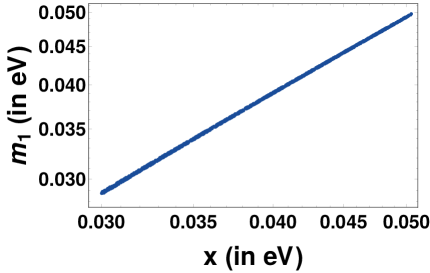
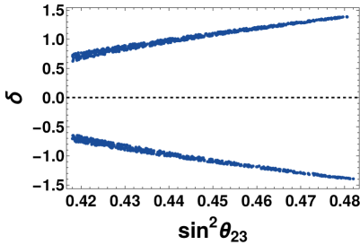
Figure 2: Correlations between different light neutrino as well as model parameters for 3$\sigma$ allowed ranges of $\theta_{13}$, $\theta_{12}$, $\theta_{23}$, mass squared differences Esteban et al. (2017) and $\sum m_{i}\leq 0.17$ eV. Left panel: the lightest neutrino mass is shown as a function of model parameter $x$. Right panel: the predicted correlation between Dirac CP phase $\delta$ and atmospheric mixing angle $\theta_{23}$.

FIMP interactions: After studying the neutrino sector, we briefly comment upon the Yukawa Lagrangian involving the FIMP dark matter candidate $\psi$ upto dimension six level. From the field content shown in Table 1, it is obvious that a bare mass term for $\psi$ is not allowed. However, we can generate its mass at dimension five level (same as that of charged leptons). The corresponding Yukawa Lagrangian is

$$\mathcal{L}_{\psi\zeta}=\frac{1}{2}Y_{\psi\zeta}\frac{\zeta^{2}}{\Lambda}\psi\psi.$$ (54)

Once $\zeta$ acquires a non-zero vev, we can generate a mass $M_{\psi}=Y_{\psi\zeta}\frac{\langle\zeta\rangle^{2}}{\Lambda}$. Another important Yukawa interaction of $\psi$ is with the singlet flavon $\eta$ that arises at dimension six level, given by

$$\mathcal{L}_{\psi\eta} = \frac{(\phi_{S})^{2}}{\Lambda^{2}}\eta\psi\psi$$ (55)

$$= \frac{v_{S_{1}}^{2}+v_{S_{2}}^{2}+v_{S_{3}}^{2}}{\Lambda^{2}}\eta\psi\psi~{}~{}{\text{for}}~{}~{}\langle\phi_{S}\rangle=(v_{S_{1}},v_{S_{2}},v_{S_{3}})$$ (56)

$$= \frac{3v_{S}^{2}}{\Lambda^{2}}\eta\psi\psi~{}~{}{\text{for}}~{}~{}\langle\phi_{S}\rangle=(v_{S},v_{S},v_{S})$$ (57)

$$= \frac{2v_{S}^{2}}{\Lambda^{2}}\eta\psi\psi~{}~{}{\text{for}}~{}~{}\langle\phi_{S}\rangle=(v_{S},v_{S},0),(v_{S},0,v_{S}),~{}{\rm or}~{}(0,v_{S},v_{S})$$ (58)

It is interesting to note that the same flavon field $\phi_{S}$ and the ratio $\frac{\langle\phi_{S}\rangle^{2}}{\Lambda^{2}}$ generates the effective coupling of $\eta-\psi-\psi$ as well as $H-\nu_{L}-\nu_{R}$ as discussed earlier in equation (II). We will use these interactions while discussing the dark matter phenomenology in the next section.

III Freeze-in Dark Matter

In this section, we discuss the details of calculation related to the relic abundance of FIMP dark matter candidate $\psi$. As per requirement for such dark matter Hall et al. (2010), the interactions of dark matter particle with the visible sector ones are so feeble that it never attains thermal equilibrium in the early Universe. In the simplest possible scenario of this type, the dark matter candidate has negligible initial thermal abundance and gets populated later due to the decay of a mother particle. Such non-thermal dark matter scenario which gets populated in the Universe through freeze-in (rather than freeze-out of WIMP type scenarios) should have typical coupling of the order $10^{-12}$ with the decaying mother particle. Unless such decays of mother particles into dark matter are kinematically forbidden, the contributions of scattering to freeze-in of dark matter remains typically suppressed compared to the former.

In our model, the fermion $\psi$ naturally satisfies the criteria for being a FIMP dark matter candidate without requiring highly fine-tuned couplings mentioned above. This is due to the fact that this fermion is a gauge singlet and its leading order interaction to the mother particle $\eta$ arises only at dimension six level. As discussed in the previous section, the effective Yukawa coupling for $\eta\psi\psi$ interaction is dynamically generated by flavon vev’s $Y\sim\frac{v^{2}_{S}}{\Lambda^{2}}$. Now, the decay width of $\eta$ into two dark matter particles $(\psi)$ can be written as

$$\Gamma_{\eta\rightarrow\psi\psi}=\frac{Y^{2}\left(m_{\eta}^{2}-4m_{\psi}^{2}\right)\sqrt{1-\frac{4m_{\psi}^{2}}{m_{\eta}^{2}}}}{8\pi m_{\eta}}$$ (59)

where Y is the effective Yukawa coupling, m_η and m_ψ are the masses of the mother particle and $\psi$ respectively. From the transformation of the singlet scalar $\eta$ under the symmetry group of the model, it is clear that it does not have any linear term in the scalar sector and hence does not have any other decay modes apart from the one into two dark matter particles. Since this decay is governed by a tiny effective Yukawa coupling, this makes the singlet scalar long lived. However, this singlet scalar can have sizeable quartic interactions with other scalars like the standard model Higgs doublet and hence can be thermally produced in the early Universe. Now, considering the mother particle $\eta$ to be in thermal equilibrium in the early Universe which also decays into the dark matter particle $\psi$, we can write down the relevant Boltzmann equations for co-moving number densities of $\eta,\psi$ as

$$\frac{dY_{\eta}}{dx} = -\frac{4\pi^{2}}{45}\frac{M_{\rm Pl}M_{\rm sc}}{1.66}\frac{\sqrt{g_{\star}(x)}}{x^{2}}\Bigg{[}\sum_{p\,=\,\text{SM\, particles}}\langle\sigma{\rm v}\rangle_{\eta\eta\rightarrow p\bar{p}}\left(Y_{\eta}^{2}-(Y_{\eta}^{\rm eq})^{2}\right)\Bigg{]}$$ (60)

$$-\frac{M_{\rm Pl}}{1.66}\frac{x\sqrt{g_{\star}(x)}}{M_{\rm sc}^{2}\ g_{s}(x)}\Gamma_{\eta\rightarrow\bar{\psi}\psi}\ Y_{\eta},$$

$$\frac{dY_{\psi}}{dx} = \frac{2M_{\rm Pl}}{1.66}\frac{x\sqrt{g_{\star}(x)}}{M_{\rm sc}^{2}\ g_{s}(x)}\Gamma_{\eta\rightarrow\bar{\psi}\psi}\ Y_{\eta}$$ (61)

where $x=\dfrac{M_{\rm sc}}{T}$, is a dimensionless variable while $M_{\rm sc}$ is some arbitrary mass scale which we choose equal to the mass of $\eta$ and $M_{\rm Pl}$ is the Planck mass. Moreover, $g_{s}(x)$ is the number of effective degrees of freedom associated to the entropy density of the Universe and the quantity $g_{\star}(x)$ is defined as

$$\sqrt{g_{\star}(x)}=\dfrac{g_{\rm s}(x)}{\sqrt{g_{\rho}(x)}}\,\left(1-\dfrac{1}{3}\dfrac{{\rm d}\,{\rm ln}\,g_{\rm s}(x)}{{\rm d}\,{\rm ln}x}\right)\,.$$ (62)

Here, $g_{\rho}(x)$ denotes the effective number of degrees of freedom related to the energy density of the Universe at $x=\dfrac{M_{\rm sc}}{T}$. The first term on the right hand side of the Boltzmann equation (60) corresponds to the self annihilation of $\eta$ into standard model particles and vice versa which play the role in its freeze-out. The second term on the right hand side of this equation corresponds to the dilution of $\eta$ due to its decay into dark matter $\psi$. Let us denote the freeze-out temperature of $\eta$ as $T_{F}$ and its decay temperature as $T_{D}$. If we assume that the mother particle freezes out first followed by its decay into dark matter particles, we can consider $T_{F}>T_{D}$. In such a case, we can first solve the Boltzmann equation for $\eta$ considering only the self-annihilation part to calculate its freeze-out abundance.

$$\frac{dY_{\eta}}{dx} = -\frac{4\pi^{2}}{45}\frac{M_{\rm Pl}M_{\rm sc}}{1.66}\frac{\sqrt{g_{\star}(x)}}{x^{2}}\Bigg{[}\sum_{p\,=\,\text{SM\, particles}}\langle\sigma{\rm v}\rangle_{\eta\eta\rightarrow p\bar{p}}\left(Y_{\eta}^{2}-(Y_{\eta}^{\rm eq})^{2}\right)\Bigg{]}$$ (63)

Then we solve the following two equations for temperature $T<T_{F}$

$$\frac{dY_{\eta}}{dx} = -\frac{M_{\rm Pl}}{1.66}\frac{x\sqrt{g_{\star}(x)}}{M_{\rm sc}^{2}\ g_{s}(x)}\Gamma_{\eta\rightarrow\bar{\psi}\psi}\ Y_{\eta},$$ (64)

$$\frac{dY_{\psi}}{dx} = \frac{2M_{\rm Pl}}{1.66}\frac{x\sqrt{g_{\star}(x)}}{M_{\rm sc}^{2}\ g_{s}(x)}\Gamma_{\eta\rightarrow\bar{\psi}\psi}\ Y_{\eta}.$$ (65)

We stick to this simplified assumption $T_{F}>T_{D}$ in this work and postpone a more general analysis without any assumption to an upcoming work. The assumption $T_{F}>T_{D}$ allows us to solve the Boltzmann equation (63) for $\eta$ first, calculate its freeze-out abundance and then solve the corresponding equations (64), (65) for $\eta,\psi$ using the freeze-out abundance of $\eta$ as initial condition. In such a scenario, we can solve the Boltzmann equations (64), (65) for different benchmark choices of $Y,m_{\eta},m_{\rm DM}\equiv M_{\psi}$ and estimate the freeze-out abundance of $\eta$ that can generate $\Omega h^{2}=0.12$, the canonical value of the dark matter $(\psi)$ relic abundance in the present Universe. This required freeze-out abundance of $\eta$ then restricts the parameters involved in its coupling to the SM particles. It turns out that a scalar singlet like $\eta$ interacts with the SM particles only through the Higgs portal and hence depends upon the $\eta-H$ coupling, denoted by $\lambda_{H\eta}$. In figure 3, we show different benchmark scenarios that give rise to the correct relic abundance of dark matter. In the left panel of figure 3, we show the abundance of both $\eta$ (after its thermal freeze-out) and $\psi$ for benchmark values of their masses $(m_{\eta}=200\;\text{GeV},m_{\rm DM}=1\;\text{GeV})$ as a function of temperature for three different values of Yukawa coupling $Y=10^{-13},10^{-12},10^{-11}$. It can be clearly seen that while the freeze-out abundance of $\eta$ drops due to its decay into $\psi$, the abundance of the latter grows. The value of $\eta-H$ coupling is chosen to be $\lambda_{H\eta}=0.004$ in order to generate the correct freeze-out abundance of $\eta$ which can later give rise to the required dark matter abundance through its decay. It can be seen that, once we fix the $\psi$ and $\eta$ masses, the final abundance of $\psi$ does not depend upon the specific Yukawa coupling $Y$ as $\eta$ dominantly decays into $\psi$ only. However, different values of $Y$ can lead to different temperatures at which the freeze-in of $\psi$ occurs, as seen from the left panel of figure 3. The right panel of figure 3 shows the relic abundance of dark matter for a fixed value of Yukawa coupling $Y=10^{-12}$ but three different benchmark choices of $m_{\eta},m_{\rm DM}$ where the $\lambda_{H\eta}$ parameter is chosen appropriately in each case so as to generate the correct freeze-out abundance of $\eta$.

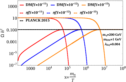
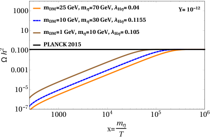
Figure 3: Left panel: Relic abundance of $\eta$ and dark matter $(\psi)$ as a function of temperature for different benchmark values of Yukawa coupling $Y$. Right panel: Relic abundance of dark matter $(\psi)$ as a function of temperature for different benchmark values of $\psi$ and $\eta$ masses and fixed Yukawa $Y=10^{-12}$.

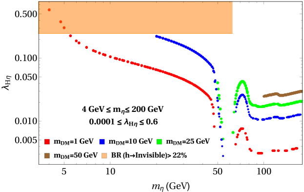
Figure 4: The allowed parameter space in $\lambda_{H\eta}$-m_η plane for different DM masses which gives rise to the required freeze-out abundance of $\eta$ followed by the correct DM abundance from $\eta$ decay.

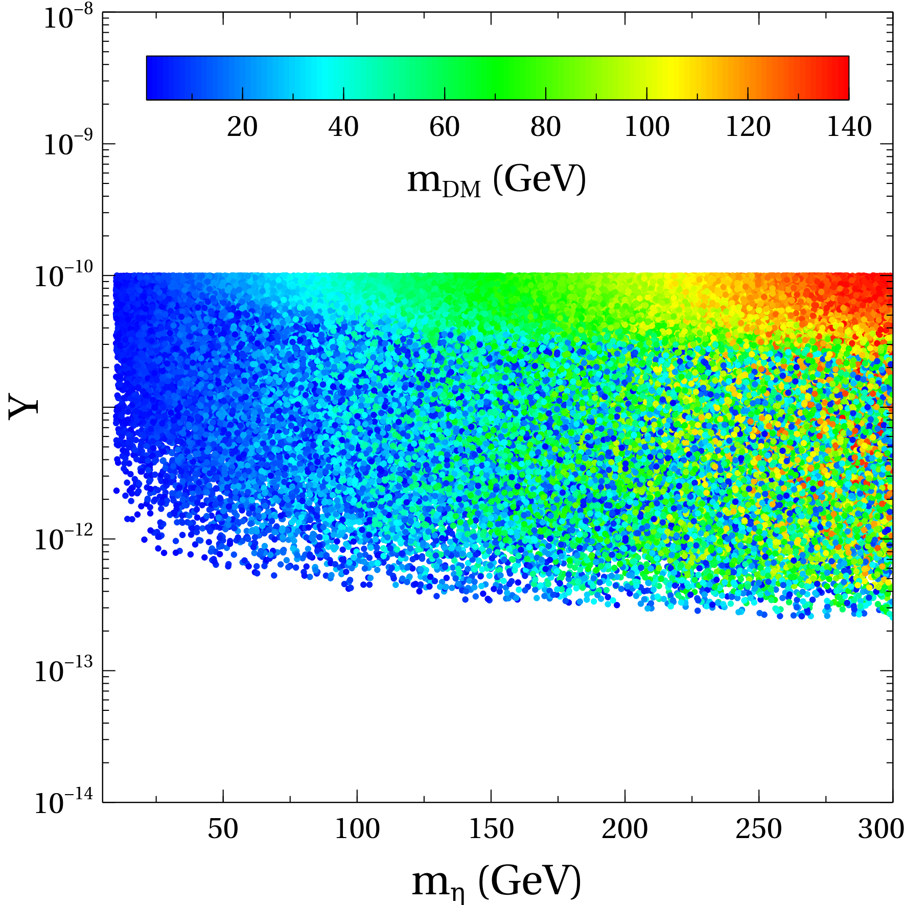
Figure 5: Parameter space for Yukawa coupling and $\eta$-DM masses that satisfy the upper and lower bounds on lifetime of $\eta:T_{\rm BBN}<T_{D}<T_{F}$.

The freeze-out abundance of $\eta$ can be calculated similar to the way the relic abundance of scalar singlet dark matter is calculated. For the details of scalar singlet dark matter, one may refer to the recent article Athron et al. (2017) and references therein for earlier works. In figure 4, we show the parameter space of scalar singlet $\eta$ in terms of $\lambda_{H\eta},m_{\eta}$ that can give rise to the required freeze-out abundance in order to generate the correct FIMP abundance through $\eta\rightarrow\psi\psi$ decay. In this plot, the resonance region is clearly visible at $m_{\eta}=m_{h}/2$ where $m_{h}\approx 125$ GeV is the SM like Higgs boson. The parameter space corresponding to DM mass of 50 GeV is seen only at the extreme right end of the plot in figure 4 due to the requirement of $m_{\eta}\geq 2m_{\rm DM}$ to enable the decay of $\psi$ into two DM candidates. Since $\eta$ is long lived and it decays only into DM at leading order, any production of $\eta$ at experiments like the LHC could be probed through invisible decay of SM like Higgs. However, this constraint is applicable only for dark matter mass $m_{\eta}<m_{h}/2$. The invisible decay width is given by

$$\Gamma(h\rightarrow\text{Invisible})={\lambda^{2}_{H\eta}v^{2}\over 64\pi m_{h}}\sqrt{1-4\,m^{2}_{\eta}/m^{2}_{h}}$$ (66)

The latest constraint on invisible Higgs decay from the ATLAS experiment at the LHC is Aad et al. (2015)

$$\text{BR}(h\rightarrow\text{Invisible})=\frac{\Gamma(h\rightarrow\text{Invisible})}{\Gamma(h\rightarrow\text{Invisible})+\Gamma(h\rightarrow\text{SM})}<22\%.$$

We incorporate this in figure 4 and find that some part of parameter space in $\lambda_{H\eta}$-m_η plane can be excluded for low dark matter masses $m_{\rm DM}<10$ GeV by LHC constraints.

Although we are considering a simplified case where the decay of mother particle occurs after the mother particle freezes out $T_{F}>T_{D}$, we note that this decay can not be delayed indefinitely. Considering the successful predictions of big bang nucleosynthesis (BBN) which occurs around typical time scale $t\sim 1\;\text{s}$, we constrain the lifetime of $\eta$ to be less than this BBN epoch so as not to alter the cosmology post-BBN era. The upper and lower bound on $\eta$ lifetime therefore, constrains the corresponding Yukawa which we show as a scan plot in figure 5 for different values of $\eta$ and dark matter masses. Dark matter masses are also varied in such a way that $m_{\eta}\geq 2m_{\rm DM}$ is satisfied. We have not incorporated the constraints on dark matter relic abundance in figure 5, as we still have freedom in choosing $\lambda_{H\eta}$ that can decide the freeze-out abundance of $\eta$ required for producing correct dark matter abundance through freeze-in. We leave a more general scan of such parameter space to an upcoming work.

It should be noted that we did not consider the production of dark matter from the decay of the flavon $\zeta$ responsible for its mass, as shown in equation (54). Since we intended to explain FIMP coupling and Dirac neutrino mass through same dimension six couplings, we did not take this dimension five term into account. This can be justified if we consider the masses of such flavons to be larger than the reheat temperature of the Universe, so that any contribution to FIMP production from $\zeta$ decay is Boltzmann suppressed. For example, the authors of Mambrini et al. (2013) considered such heavy mediators having mass greater than the reheat temperature, in a different dark matter scenario. We also note that there was no contribution to FIMP production through annihilations in our scenario through processes like ${\rm SM,SM}\rightarrow\psi\psi$ with $\eta$ being the mediator. This is justified due to the specific flavour transformations of $\eta$ and the fact that $\eta$ does not acquire any vev.

IV Conclusion

We have proposed a scenario that can simultaneously explain the tiny Yukawa coupling required for Dirac neutrino masses from the standard model Higgs field and the coupling of non-thermal dark matter populating the Universe through freeze-in mechanism. The proposed scenario is based on dynamical origin of such tiny couplings from a flavour symmetric scenario based on discrete non-abelian group $A_{4}$ that allows such couplings at dimension six level only thereby explaining their smallness naturally. The $A_{4}$ flavour symmetry is augmented by additional discrete symmetries like $Z_{N}$ and a global lepton number symmetry to forbid the unwanted terms from the Lagrangian. The charged lepton and dark matter masses are generated at dimension five level while the sub-eV Dirac neutrino masses arise only at dimension six level. The correct leptonic mixing can be produced depending on the alignment of flavon vev’s. One such alignment which we analyse numerically predicts a normal hierarchical pattern of light neutrino masses and interesting correlations between neutrino oscillation parameters. The atmospheric mixing angle is preferred to be in the lower octant for maximal Dirac CP phase in this scenario.

In the dark matter sector, the effective coupling of non-thermal dark matter ($\psi$, a singlet fermion) with its mother particle ($\eta$, a singlet scalar) arises at dimension six level through the same flavons responsible for neutrino mass. The mother particle, though restricted to decay only to the dark matter particles at cosmological scales, can have sizeable interactions with the standard model sector through Higgs portal couplings. Adopting a simplified scenario where the mother particle freezes out first and then decays into the dark matter particles, we first calculate the freeze-out abundance of $\eta$ and then calculate the dark matter abundance from $\eta$ decay. Although such non-thermal or freeze-in massive particle dark matter remains difficult to be probed due to tiny couplings, its mother particle can be produced at ongoing experiments like the LHC. We in fact show that some part of mother particle’s parameter space can be constrained from the LHC limits on invisible decay rate of the SM like Higgs boson, and hence can be probed in near future data. Since $\eta$ is long lived, its decay into dark matter particles on cosmological scales can be constrained if we demand such a decay to occur before the BBN epoch. We find the lower bound on Yukawa coupling $Y$ governing the decay of $\eta$ into DM, and show it to be larger than around $10^{-13}$. We leave a more detailed analysis of such scenario without any assumption of $\eta$ freeze-out preceding the freeze-in of $\psi$ to an upcoming work.

Appendix A $A_{4}$ Multiplication Rules

$A_{4}$, the symmetry group of a tetrahedron, is a discrete non-abelian group of even permutations of four objects. It has four irreducible representations: three one-dimensional and one three dimensional which are denoted by $\bf{1},\bf{1^{\prime}},\bf{1^{\prime\prime}}$ and $\bf{3}$ respectively, being consistent with the sum of square of the dimensions $\sum_{i}n_{i}^{2}=12$. We denote a generic permutation $(1,2,3,4)\rightarrow(n_{1},n_{2},n_{3},n_{4})$ simply by $(n_{1}n_{2}n_{3}n_{4})$. The group $A_{4}$ can be generated by two basic permutations $S$ and $T$ given by $S=(4321),T=(2314)$. This satisfies

$$S^{2}=T^{3}=(ST)^{3}=1$$

which is called a presentation of the group. Their product rules of the irreducible representations are given as

$$\bf{1}\otimes\bf{1}=\bf{1}$$

$$\bf{1^{\prime}}\otimes\bf{1^{\prime}}=\bf{1^{\prime\prime}}$$

$$\bf{1^{\prime}}\otimes\bf{1^{\prime\prime}}=\bf{1}$$

$$\bf{1^{\prime\prime}}\otimes\bf{1^{\prime\prime}}=\bf{1^{\prime}}$$

$$\bf{3}\otimes\bf{3}=\bf{1}\otimes\bf{1^{\prime}}\otimes\bf{1^{\prime\prime}}\otimes\bf{3}_{a}\otimes\bf{3}_{s}$$

where $a$ and $s$ in the subscript corresponds to anti-symmetric and symmetric parts respectively. Denoting two triplets as $(a_{1},b_{1},c_{1})$ and $(a_{2},b_{2},c_{2})$ respectively, their direct product can be decomposed into the direct sum mentioned above. In the $S$ diagonal basis, the products are given as

$$\bf{1}\backsim a_{1}a_{2}+b_{1}b_{2}+c_{1}c_{2}$$

$$\bf{1^{\prime}}\backsim a_{1}a_{2}+\omega^{2}b_{1}b_{2}+\omega c_{1}c_{2}$$

$$\bf{1^{\prime\prime}}\backsim a_{1}a_{2}+\omega b_{1}b_{2}+\omega^{2}c_{1}c_{2}$$

$$\bf{3}_{s}\backsim(b_{1}c_{2}+c_{1}b_{2},c_{1}a_{2}+a_{1}c_{2},a_{1}b_{2}+b_{1}a_{2})$$

$$\bf{3}_{a}\backsim(b_{1}c_{2}-c_{1}b_{2},c_{1}a_{2}-a_{1}c_{2},a_{1}b_{2}-b_{1}a_{2})$$

In the $T$ diagonal basis on the other hand, they can be written as

$$\bf{1}\backsim a_{1}a_{2}+b_{1}c_{2}+c_{1}b_{2}$$

$$\bf{1^{\prime}}\backsim c_{1}c_{2}+a_{1}b_{2}+b_{1}a_{2}$$

$$\bf{1^{\prime\prime}}\backsim b_{1}b_{2}+c_{1}a_{2}+a_{1}c_{2}$$

$$\bf{3}_{s}\backsim\frac{1}{3}(2a_{1}a_{2}-b_{1}c_{2}-c_{1}b_{2},2c_{1}c_{2}-a_{1}b_{2}-b_{1}a_{2},2b_{1}b_{2}-a_{1}c_{2}-c_{1}a_{2})$$

$$\bf{3}_{a}\backsim\frac{1}{2}(b_{1}c_{2}-c_{1}b_{2},a_{1}b_{2}-b_{1}a_{2},c_{1}a_{2}-a_{1}c_{2})$$

References

- Patrignani et al. (2016) C. Patrignani et al. (Particle Data Group), Chin. Phys. C40, 100001 (2016).
- Esteban et al. (2017) I. Esteban, M. C. Gonzalez-Garcia, M. Maltoni, I. Martinez-Soler, and T. Schwetz, JHEP 01, 087 (2017), eprint 1611.01514.
- de Salas et al. (2017) P. F. de Salas, D. V. Forero, C. A. Ternes, M. Tortola, and J. W. F. Valle (2017), eprint 1708.01186.
- Ade et al. (2016) P. A. R. Ade et al. (Planck), Astron. Astrophys. 594, A13 (2016), eprint 1502.01589.
- Zwicky (1933) F. Zwicky, Helv. Phys. Acta 6, 110 (1933), [Gen. Rel. Grav.41,207(2009)].
- Rubin and Ford (1970) V. C. Rubin and W. K. Ford, Jr., Astrophys. J. 159, 379 (1970).
- Clowe et al. (2006) D. Clowe, M. Bradac, A. H. Gonzalez, M. Markevitch, S. W. Randall, C. Jones, and D. Zaritsky, Astrophys. J. 648, L109 (2006), eprint astro-ph/0608407.
- Hinshaw et al. (2013) G. Hinshaw et al. (WMAP), Astrophys. J. Suppl. 208, 19 (2013), eprint 1212.5226.
- Minkowski (1977) P. Minkowski, Phys. Lett. B67, 421 (1977).
- Gell-Mann et al. (1979) M. Gell-Mann, P. Ramond, and R. Slansky, Conf. Proc. C790927, 315 (1979), eprint 1306.4669.
- Mohapatra and Senjanovic (1980) R. N. Mohapatra and G. Senjanovic, Phys. Rev. Lett. 44, 912 (1980).
- Schechter and Valle (1980) J. Schechter and J. W. F. Valle, Phys. Rev. D22, 2227 (1980).
- Tan et al. (2016) A. Tan et al. (PandaX-II), Phys. Rev. Lett. 117, 121303 (2016), eprint 1607.07400.
- Aprile et al. (2017) E. Aprile et al. (XENON), Phys. Rev. Lett. 119, 181301 (2017), eprint 1705.06655.
- Akerib et al. (2017) D. S. Akerib et al. (LUX), Phys. Rev. Lett. 118, 021303 (2017), eprint 1608.07648.
- Hall et al. (2010) L. J. Hall, K. Jedamzik, J. March-Russell, and S. M. West, JHEP 03, 080 (2010), eprint 0911.1120.
- Biswas and Gupta (2016) A. Biswas and A. Gupta, JCAP 1609, 044 (2016), [Addendum: JCAP1705,no.05,A01(2017)], eprint 1607.01469.
- Biswas et al. (2017) A. Biswas, S. Choubey, and S. Khan, Eur. Phys. J. C77, 875 (2017), eprint 1704.00819.
- Bernal et al. (2017) N. Bernal, M. Heikinheimo, T. Tenkanen, K. Tuominen, and V. Vaskonen, Int. J. Mod. Phys. A32, 1730023 (2017), eprint 1706.07442.
- Babu and He (1989) K. S. Babu and X. G. He, Mod. Phys. Lett. A4, 61 (1989).
- Peltoniemi et al. (1993) J. T. Peltoniemi, D. Tommasini, and J. W. F. Valle, Phys. Lett. B298, 383 (1993).
- Centelles Chuliá et al. (2017a) S. Centelles Chuliá, E. Ma, R. Srivastava, and J. W. F. Valle, Phys. Lett. B767, 209 (2017a), eprint 1606.04543.
- Aranda et al. (2014) A. Aranda, C. Bonilla, S. Morisi, E. Peinado, and J. W. F. Valle, Phys. Rev. D89, 033001 (2014), eprint 1307.3553.
- Chen et al. (2016) P. Chen, G.-J. Ding, A. D. Rojas, C. A. Vaquera-Araujo, and J. W. F. Valle, JHEP 01, 007 (2016), eprint 1509.06683.
- Ma et al. (2015) E. Ma, N. Pollard, R. Srivastava, and M. Zakeri, Phys. Lett. B750, 135 (2015), eprint 1507.03943.
- Reig et al. (2016) M. Reig, J. W. F. Valle, and C. A. Vaquera-Araujo, Phys. Rev. D94, 033012 (2016), eprint 1606.08499.
- Wang and Han (2016) W. Wang and Z.-L. Han (2016), [JHEP04,166(2017)], eprint 1611.03240.
- Wang et al. (2017) W. Wang, R. Wang, Z.-L. Han, and J.-Z. Han, Eur. Phys. J. C77, 889 (2017), eprint 1705.00414.
- Wang et al. (2006) F. Wang, W. Wang, and J. M. Yang, Europhys. Lett. 76, 388 (2006), eprint hep-ph/0601018.
- Gabriel and Nandi (2007) S. Gabriel and S. Nandi, Phys. Lett. B655, 141 (2007), eprint hep-ph/0610253.
- Davidson and Logan (2009) S. M. Davidson and H. E. Logan, Phys. Rev. D80, 095008 (2009), eprint 0906.3335.
- Davidson and Logan (2010) S. M. Davidson and H. E. Logan, Phys. Rev. D82, 115031 (2010), eprint 1009.4413.
- Bonilla and Valle (2016) C. Bonilla and J. W. F. Valle, Phys. Lett. B762, 162 (2016), eprint 1605.08362.
- Farzan and Ma (2012) Y. Farzan and E. Ma, Phys. Rev. D86, 033007 (2012), eprint 1204.4890.
- Bonilla et al. (2016) C. Bonilla, E. Ma, E. Peinado, and J. W. F. Valle, Phys. Lett. B762, 214 (2016), eprint 1607.03931.
- Ma and Popov (2017) E. Ma and O. Popov, Phys. Lett. B764, 142 (2017), eprint 1609.02538.
- Ma and Sarkar (2018) E. Ma and U. Sarkar, Phys. Lett. B776, 54 (2018), eprint 1707.07698.
- Borah (2016) D. Borah, Phys. Rev. D94, 075024 (2016), eprint 1607.00244.
- Borah and Dasgupta (2016) D. Borah and A. Dasgupta, JCAP 1612, 034 (2016), eprint 1608.03872.
- Borah and Dasgupta (2017a) D. Borah and A. Dasgupta, JHEP 01, 072 (2017a), eprint 1609.04236.
- Borah and Dasgupta (2017b) D. Borah and A. Dasgupta, JCAP 1706, 003 (2017b), eprint 1702.02877.
- Centelles Chuliá et al. (2017b) S. Centelles Chuliá, R. Srivastava, and J. W. F. Valle, Phys. Lett. B773, 26 (2017b), eprint 1706.00210.
- Bonilla et al. (2018) C. Bonilla, J. M. Lamprea, E. Peinado, and J. W. F. Valle, Phys. Lett. B779, 257 (2018), eprint 1710.06498.
- Memenga et al. (2013) N. Memenga, W. Rodejohann, and H. Zhang, Phys. Rev. D87, 053021 (2013), eprint 1301.2963.
- Borah and Karmakar (2018) D. Borah and B. Karmakar, Phys. Lett. B780, 461 (2018), eprint 1712.06407.
- Centelles Chuliá et al. (2018a) S. Centelles Chuliá, R. Srivastava, and J. W. F. Valle, Phys. Lett. B781, 122 (2018a), eprint 1802.05722.
- Centelles Chuliá et al. (2018b) S. Centelles Chuliá, R. Srivastava, and J. W. F. Valle (2018b), eprint 1804.03181.
- Han and Wang (2018) Z.-L. Han and W. Wang (2018), eprint 1805.02025.
- Elahi et al. (2015) F. Elahi, C. Kolda, and J. Unwin, JHEP 03, 048 (2015), eprint 1410.6157.
- McDonald (2016) J. McDonald, JCAP 1608, 035 (2016), eprint 1512.06422.
- Biswas et al. (2018) A. Biswas, D. Borah, and A. Dasgupta (2018), eprint 1805.06903.
- Gopalakrishna et al. (2006) S. Gopalakrishna, A. de Gouvea, and W. Porod, JCAP 0605, 005 (2006), eprint hep-ph/0602027.
- de Gouvea et al. (2006) A. de Gouvea, S. Gopalakrishna, and W. Porod, JHEP 11, 050 (2006), eprint hep-ph/0606296.
- Page (2007) V. Page, JHEP 04, 021 (2007), eprint hep-ph/0701266.
- Asaka et al. (2007) T. Asaka, K. Ishiwata, and T. Moroi, Phys. Rev. D75, 065001 (2007), eprint hep-ph/0612211.
- Asaka et al. (2006) T. Asaka, K. Ishiwata, and T. Moroi, Phys. Rev. D73, 051301 (2006), eprint hep-ph/0512118.
- Borah et al. (2017) D. Borah, M. K. Das, and A. Mukherjee (2017), eprint 1711.02445.
- Karmakar and Sil (2015) B. Karmakar and A. Sil, Phys. Rev. D91, 013004 (2015), eprint 1407.5826.
- He et al. (2006) X.-G. He, Y.-Y. Keum, and R. R. Volkas, JHEP 04, 039 (2006), eprint hep-ph/0601001.
- Branco et al. (2009) G. C. Branco, R. Gonzalez Felipe, M. N. Rebelo, and H. Serodio, Phys. Rev. D79, 093008 (2009), eprint 0904.3076.
- Lin (2009) Y. Lin, Nucl. Phys. B813, 91 (2009), eprint 0804.2867.
- Dorame et al. (2012) L. Dorame, S. Morisi, E. Peinado, J. W. F. Valle, and A. D. Rojas, Phys. Rev. D86, 056001 (2012), eprint 1203.0155.
- Rodejohann and Xu (2016) W. Rodejohann and X.-J. Xu, Eur. Phys. J. C76, 138 (2016), eprint 1509.03265.
- Grimus and Lavoura (2008) W. Grimus and L. Lavoura, JHEP 09, 106 (2008), eprint 0809.0226.
- Albright and Rodejohann (2009) C. H. Albright and W. Rodejohann, Eur. Phys. J. C62, 599 (2009), eprint 0812.0436.
- Albright et al. (2010) C. H. Albright, A. Dueck, and W. Rodejohann, Eur. Phys. J. C70, 1099 (2010), eprint 1004.2798.
- He and Zee (2011) X.-G. He and A. Zee, Phys. Rev. D84, 053004 (2011), eprint 1106.4359.
- Borah and Gupta (2017) D. Borah and A. Gupta, Phys. Rev. D96, 115012 (2017), eprint 1706.05034.
- Athron et al. (2017) P. Athron et al. (GAMBIT), Eur. Phys. J. C77, 568 (2017), eprint 1705.07931.
- Aad et al. (2015) G. Aad et al. (ATLAS), JHEP 11, 206 (2015), eprint 1509.00672.
- Mambrini et al. (2013) Y. Mambrini, K. A. Olive, J. Quevillon, and B. Zaldivar, Phys. Rev. Lett. 110, 241306 (2013), eprint 1302.4438.