Bayesian Model Comparison and Analysis of the Galactic Disk Population of Gamma-Ray Millisecond Pulsars

Abstract

Pulsed emission from almost one hundred millisecond pulsars (MSPs) has been detected in $\gamma$-rays by the Fermi Large-Area Telescope. The global properties of this population remain relatively unconstrained despite many attempts to model their spatial and luminosity distributions. We perform here a self-consistent Bayesian analysis of both the spatial distribution and luminosity function simultaneously. Distance uncertainties, arising from errors in the parallax measurement or Galactic electron-density model, are marginalized over. We provide a public Python package for calculating distance uncertainties to pulsars derived using the dispersion measure by accounting for the uncertainties in Galactic electron-density model YMW16. Finally, we use multiple parameterizations for the MSP population and perform Bayesian model comparison, finding that a broken power law luminosity function with Lorimer spatial profile are preferred over multiple other parameterizations used in the past. The best-fit spatial distribution and number of $\gamma$-ray MSPs is consistent with results for the radio population of MSPs.

1 Introduction

Millisecond pulsars (MSPs) are believed to be recycled pulsars that are spun-up to millisecond periods by accreting matter from a companion star (Bhattacharya & van den Heuvel, 1991). Prior to the launch of the Fermi Gamma-Ray Space Telescope pulsations from only one MSP had been claimed in $\gamma$-rays and at low statistical significance (Kuiper et al., 2000). Since then the Large Area Telescope (LAT) aboard Fermi has revolutionized the field with close to one hundred $\gamma$-ray detected millisecond pulsars (Caraveo, 2014; Abdo et al., 2009a, b, 2013). Most detections of $\gamma$-ray pulsations in MSPs follow from phase-folding the timing parameters already known from radio (e.g.  Abdo et al., 2009b). In many cases, the radio MSPs have been initially detected during follow-up observations of Fermi unassociated sources after which the timing information is utilized to confirm $\gamma$-ray pulsations (e.g.  Cognard et al., 2011). Increased computing power has made it possible to detect $\gamma$-ray pulsations in blind searches where no timing information is available (Pletsch et al., 2012; Clark et al., 2018).

Population studies of MSPs in radio have constrained their spatial distribution, luminosity function and the number of radio-emitting MSPs in the Galactic disk (Cordes & Chernoff, 1997; Lyne et al., 1998; Levin et al., 2013). On the other hand, $\gamma$-ray population studies of MSPs have been performed to constrain their luminosity function and in some cases their spatial distribution (Hooper et al., 2013; Grégoire & Knödlseder, 2013; Yuan & Zhang, 2014; Cholis et al., 2014; Hooper & Mohlabeng, 2016; Winter et al., 2016; Ploeg et al., 2017).

A particular goal of many of these analyses has been to rule-out or constrain the MSP interpretation of the Fermi Galactic Center Excess (GCE). The GCE is an excess of $\gamma$-rays at energies of $\sim 2\mathrm{\,GeV}$ that is spatially coincident with the Galactic Bulge (Goodenough & Hooper, 2009; Daylan et al., 2016; Calore et al., 2015) and was also shown to be morphologically similar (Bartels et al., 2017). It has been suggested that the GCE could be caused by a bulge population of MSPs (Abazajian, 2011; Gordon & Macias, 2013). Corroborative evidence for this scenario was found by analysing the photon statistics of the inner-Galaxy (Lee et al., 2016; Bartels et al., 2016). However, arguments against this scenario exist based on an apparent conflict between the luminosity function of MSPs in the Galactic disk and the intensity of the GCE. It was argued that if the GCE is caused by MSPs we should have already detected a few dozen sources from this population (Hooper et al., 2013; Cholis et al., 2014; Hooper & Mohlabeng, 2016). Conversely, other studies claimed that there is no discrepancy if bulge MSPs have the same luminosity function as disk MSPs (Yuan & Zhang, 2014; Petrović et al., 2015; Ploeg et al., 2017). Previous analyses have used a variety of distributions for the luminosity function of MSPs. Moreover, they have used different treatments of the distance estimates to MSPs, which is one of the major sources of uncertainty when estimating the pulsar luminosity. In the light of conflicting conclusions caused by particular assumptions it seems important to perform a complete and unbiased analysis, presenting all sources of uncertainty clearly and adopting a conservative set of assumptions.

In this work we perform a systematic and fully self-consistent analyses of the spatial distribution and luminosity function of MSPs. We consider different luminosity functions and parameterizations of the spatial profile, performing a Bayesian-unbinned likelihood analysis to constrain the model parameters. Bayesian model comparison is then applied to select the best model. In our analysis we marginalize over the main sources of uncertainty, namely the distance to and received flux of each source. What is more, to the best of our knowledge, we for the first time construct probability distribution functions for distances derived from the dispersion measure by taking into account the uncertainties in the parameters of the electron-density models (Yao et al., 2017). Finally, we also study how the inclusion of unassociated sources can impact our results.

The layout of the paper is as follows. We first discuss our modeling and MSP data sample in Sec. 2. Results are then given in Sect. 3. Finally we discuss the implications of our results in Sect. 4 and conclude in Sect. 5.

2 Methodology and Data

In this work we perform a Bayesian-unbinned likelihood analysis in order to fully exploit the heterogeneous information available in the data sample. We first discuss the likelihood function and then address the two main areas of uncertainty, namely the distances to sources and the contribution from unassociated sources.

2.1 Likelihood

Our analysis is based on an unbinned Poisson likelihood function,

$$\mathcal{L}\left(\mathcal{D}|\mathbf{\Theta}\right)=e^{-\mu(\mathbf{\Theta})}\prod_{i}^{N_{\mathrm{obs}}}N_{\mathrm{tot}}P(\mathcal{D}_{i}|\mathbf{\Theta})\;,$$ (1)

where $\mathbf{\Theta}$ is the vector of parameter dependencies, $N_{\mathrm{obs}}$ is the number of observed MSPs, $N_{\mathrm{tot}}$ the total number of sources and $P(\mathcal{D}_{i}|\mathbf{\Theta})$ is the probability of finding a given source at Galactic position $(\ell_{i},b_{i})$, with observed flux $F_{i}$ and, if available, parallax or dispersion measure $\omega_{i}$ or $\mathrm{DM}_{i}$, i.e. $\mathcal{D}_{i}=\left\{\ell_{i},b_{i},F_{i},\kappa_{i}\right\}$ with $\kappa_{i}=\omega_{i}$ if a parallax measurement is present, or else $\kappa_{i}=\mathrm{DM}_{i}$ if a DM measurement exists. If no distance measure is present $\mathcal{D}_{i}=\left\{\ell_{i},b_{i},F_{i}\right\}$. Furthermore, $\mu(\mathbf{\Theta})$ is the expected number of observed sources and satisfies in the point of maximum likelihood the condition

$$\mu(\mathbf{\Theta}_{\mathrm{bf}})=N_{\text{obs}}\;,$$ (2)

where $\mathbf{\Theta}_{\mathrm{bf}}$ are the maximum-likelihood values for the parameters of our model. More specifically, $\mu(\mathbf{\Theta})$ and $P(\mathcal{D}_{i}|\mathbf{\Theta})$ are given by

$$\begin{split}\mu(\mathbf{\Theta})=N_{\mathrm{tot}}\sum_{j=1}^{\mathrm{N_{\mathrm{pix}}}}\frac{\Omega_{j}}{\cos{b_{j}}}\int dD\int dL\,P(L|\mathbf{\Theta})P(\ell_{j},b_{j},D|\mathbf{\Theta})P_{\mathrm{th}}\left(\frac{L}{4\pi D^{2}}\Big{|}\mathbf{\Theta},\ell_{j},b_{j}\right),\end{split}$$ (3)

$$P(\ell_{i},b_{i},F_{i},\kappa_{i}|\mathbf{\Theta})=4\pi\int dD\int dF\,D^{2}P(\ell_{i},b_{i},D|\mathbf{\Theta})P\left(L=4\pi D^{2}F|\mathbf{\Theta}\right)P_{\mathrm{th}}\left(F\right|\mathbf{\Theta},\ell_{i},b_{i})P(\kappa_{i}|D)P(F_{i}|F)$$ (4a)

$$P(\ell_{i},b_{i},F_{i}|\mathbf{\Theta})=4\pi\int dD\int dF\,D^{2}P(\ell_{i},b_{i},D|\mathbf{\Theta})P\left(L=4\pi D^{2}F|\mathbf{\Theta}\right)P_{\mathrm{th}}\left(F\right|\mathbf{\Theta},\ell_{i},b_{i})P(F_{i}|F)$$ (4b)

Here $P(L|\mathbf{\Theta})$ and $P(\ell,b,D|\mathbf{\Theta})$ are the luminosity function and spatial distribution, which are discussed in detail in sections 2.1.1 and 2.1.2 respectively. The total number of sources equals the sum of the disk ($N$) and bulge sources ($N_{\mathrm{bulge}}$), $N_{\mathrm{tot}}=N+N_{\mathrm{bulge}}$. $P_{\mathrm{th}}(F|\mathbf{\Theta},\ell,b)$ is the detection sensitivity which is defined in Eq. 10. We take the observed spatial positions to correspond to the true positions, since their uncertainties are negligible for the purpose of our analysis. On the other hand, we integrate over the true distances ($D$) and fluxes ($F$) of the sources. In Sect. 2.1.4 we discuss $P(F_{i}|F)$, the probability of measuring a flux ($F_{i}$), given the true flux of the source ($F$). Similarly, $P(\kappa_{i}|D)$ is the probability of observing a particular parallax or dispersion measure value ($\kappa_{i}$) given a true distance to the source. It is discussed separately in Sect. 2.2. Equation 4a (4b) applies to sources with (without) distance information.

In order to compute the expected number of observed sources $\mu$ we must integrate over distance, flux and spatial coordinates. The spatial integral is performed by calculating expectations on a HEALPIX grid with $\mathrm{NSIDE}=32$ (Gorski et al., 2005). In this case the number of pixels is $N_{\mathrm{pix}}=12288$ and $\Omega_{i}=1\times 10^{-3}\mathrm{\,sr}$. The integral is then straightforwardly performed by summing over all pixels. Since we integrate over solid angle rather than $\ell,b$ we divide out a factor of $\cos{b}$ in Eq. 3 which appears in $P(\ell,b,D)$. Henceforth, we drop the dependence on $\mathbf{\Theta}$ for notational purposes but note that the free parameters are clearly stated in Table. 2.1.4.

2.1.1 Luminosity function

We test four parameterizations of the luminosity function in the range $0.1$–$100\mathrm{\,GeV}$, namely a single power law with a hard cutoff (PL, Eq. 5a), single power law with super-exponential cutoff (PL exp. cutoff, Eq. 5b), broken power law (BPL, Eq. 5c) and log-normal distribution (LN, Eq. 5d).

$$\frac{dN}{dL}\propto L^{-\alpha}\qquad L\leq L_{\mathrm{max}}$$ (5a)

$$\frac{dN}{dL}\propto L^{-\alpha}e^{-(L/L_{c})^{-\beta}}$$ (5b)

$$\frac{dN}{dL}\propto\left\{\begin{split}&L^{-\alpha_{1}}\qquad L\leq L_{b}\\ &L^{-\alpha_{2}}\qquad L_{b}<L\end{split}\right.$$ (5c)

$$\frac{dN}{dL}\propto\frac{1}{L}\exp\left[-\frac{\left(\log_{10}L-\log_{10}L_{0}\right)^{2}}{2\sigma_{L}^{2}}\right]$$ (5d)

Unless specified, we fix the minimum and maximum luminosities to $L_{\mathrm{min}}=10^{30}\mathrm{\,erg\,s^{-1}}$ and $L_{\mathrm{max}}=10^{37}\mathrm{\,erg\,s^{-1}}$ respectively. The number of free parameters varies for different scans. For a single power law we have the slope ($\alpha$) and the hard-cutoff ($L_{\mathrm{max}}$). The power law with super-exponential cutoff has the slope ($\alpha$), cutoff luminosity ($L_{c}$) and $\beta$. For a broken power law we have the low and high luminosity slope along with the break luminosity, denoted $\alpha_{1}$, $\alpha_{2}$, and $L_{b}$ respectively. Finally, for the log-normal distribution we have the peak of the distribution and its width denoted $L_{0}$ and $\sigma_{L}$ respectively. All parameters and their prior ranges are given Table. 2.1.4. The probability distributions for the luminosities are directly proportional to the luminosity function $P(L)\propto dN/dL$, with $\int_{L_{\text{min}}}^{L_{\text{max}}}P(L)dL=1$.

2.1.2 Spatial profiles

We consider two different functional forms for the disk. Each density profile is defined in cylindrical coordinates ($r,z,\theta$) centered on the Galactic center. The probability of finding a source at a given location is proportional to the density profile $P(r,z,\theta)=r\,n(r,z,\theta)/N$. Using the appropriate coordinate transformation (see Appendix B) this probability can be transformed to the probability of finding a source at galactic longitude and latitude $(\ell,b)$ and at distance $D$ from the Sun: $P(\ell,b,D)=D^{2}\cos{\left(b\right)}n(r,z,\theta)/N$.

Below we discuss the two parameterizations of the disk profile considered in this work, our benchmark is the Lorimer profile (Lorimer et al., 2006). In addition, we also test a model with a gaussian radial profile (Faucher-Giguere & Loeb, 2010).

Lorimer-disk profile

The Lorimer profile has a radial distribution that is described by a gamma function, whereas the $z$ distribution follows an exponential. The number density of sources is given by (Lorimer et al., 2006):

$$\begin{split}n\left(r,z\right)=&N\frac{C^{B+2}}{4\pi R^{2}_{\odot}z_{s}e^{C}\Gamma\left(B+2\right)}\times\\ &\left(\frac{r}{R_{\odot}}\right)^{B}\exp\left[-C\left(\frac{r-R_{\odot}}{R_{\odot}}\right)\right]\times\\ &\exp\left(-\frac{|z|}{z_{s}}\right).\end{split}$$ (6)

Here $N$ is the number of disk sources, $\Gamma$ the gamma function, $B$ and $C$ are parameters that define the spatial radial profile, $z_{s}$ is scale height and $R_{\mathrm{\odot}}=8.5\mathrm{\,kpc}$ the Solar distance from the Galactic Center. The spatial parameters $B,C$ and $z_{s}$ are left free in the scan (see Table 2.1.4). We note that the Lorimer disk reduces to a spatial profile with an exponential radial profile as considered by Story et al. (2007) for $B=0$.

Gaussian radial profile

We also consider a spatial profile with an exponential disk and a Gaussian radial profile (Faucher-Giguere & Loeb, 2010):

$$n\left(r,z\right)=N\frac{1}{4\pi\sigma_{r}^{2}z_{s}}e^{-r^{2}/2\sigma_{r}^{2}}e^{-|z|/z_{s}}.$$ (7)

Bulge profile

Motivated by the GCE, we allow for the presence of a bulge population of MSPs in addition to the disk population in a subset of our scans. We model the bulge as a radial power-law with a hard cutoff at $r_{c}=3\mathrm{\,kpc}$ and fixed slope of $\Gamma=2.5$ (Calore et al., 2015; Daylan et al., 2016),

$$n(r)=N_{\mathrm{bulge}}\frac{3-\Gamma}{4\pi r_{c}^{3-\Gamma}}r^{-\Gamma}.$$ (8)

Again, $P(\ell,b,D)=D^{2}\cos\left({b}\right)n(r,\theta,\phi)/N_{bulge}$ (see Appendix B).

Recently, it was found that the GCE is better described by a morphology that traces the triaxial boxy bulge instead of a spherically-symmetric profile (Bartels et al., 2017; Macias et al., 2018). Nevertheless, we model the bulge MSP population with a radial power-law. The goal is to test whether this component is required by the data at all. We do not expect this analysis to be sensitive to the exact morphology of the bulge.

2.1.3 Detection sensitivity

We allow for some uncertainty in the Fermi detection sensitivity. Depending on the dataset we use, the true detection efficiency can be an arbitrarily complicated function. In particular for confirmed pulsars, many of which have been detected by folding in the radio pulsation period, it does not only depend on the $\gamma$-ray brightness of a source, but also on the radio properties of the pulsar population and the sensitivity of current radio telescopes. Therefore, we expect the sensitivity to be different from the Fermi detection sensitivity. Here we follow the same procedure as (Hooper & Mohlabeng, 2016; Ploeg et al., 2017) to model the detection sensitivity. The threshold flux at a given sky position is drawn from a log-normal distribution:

$$\begin{split}P&(F_{\mathrm{th}}|\ell,b)=\frac{1}{\sigma_{\mathrm{th}}F_{\mathrm{th}}\sqrt{2\pi}}\\ &\exp\left[-\frac{\left(\ln F_{\mathrm{th}}-\left(\ln(F_{\mathrm{th,\,mod.}}(\ell,b))+K_{\mathrm{th}}\right)\right)^{2}}{2\sigma_{\mathrm{th}}^{2}}\right]\;,\end{split}$$ (9)

where $F_{\mathrm{th,\,mod.}}(\ell,b)$ is the sensitivity map in Fig. 16 of Abdo et al. (2013). We have two free parameters $K_{\mathrm{th}}$ and $\sigma_{\mathrm{th}}$, respectively the normalization and width of the distribution from which $F_{\mathrm{th}}$ is drawn. A source is detected if $F\geq F_{\mathrm{th}}$, therefore

$$P_{\mathrm{th}}(F|\ell,b)\equiv P\left(F\geq F_{\mathrm{th}}|\ell,b\right)\\ =\frac{1}{2}+\frac{1}{2}\mathrm{erf}\left[\frac{\ln F-\left(\ln(F_{\mathrm{th,\,mod.}}(\ell,b))+K_{\mathrm{th}}\right)}{\sqrt{2}\sigma_{\mathrm{th}}}\right]\;.$$ (10)

2.1.4 Flux uncertainties

Energy fluxes ($0.1-100\mathrm{\,GeV}$) and their uncertainties are taken from the 2FGL (Nolan et al., 2012), 3FGL (Acero et al., 2015) or the preliminary Fermi–Lat 8-year catalog (FL8Y). The flux uncertainties are treated as Gaussian, the probability of a source having some true flux ($F$) is given by

$$P(F|F_{\mathrm{obs}})=\frac{1}{\sqrt{2\pi\sigma_{F}^{2}}}e^{-\left(F-F_{\mathrm{obs}}\right)^{2}/2\sigma_{F}^{2}},$$ (11)

where $F_{\mathrm{obs}}$ and $\sigma_{F}$ are the observed energy flux ($\geq 0.1\mathrm{\,GeV}$) and its associated uncertainty.

Parameter		prior	fixed
$\log_{10}{N}$	$\left[0,8\right]$	-
$\log_{10}{N_{\mathrm{bulge}}}$	$\left[0,8\right]$	-
Luminosity function
$\log_{10}L_{\mathrm{min}}$	-	$30$
$\log_{10}L_{\mathrm{max}}$	$(\left[33.7,37\right])$	$37$
$\log_{10}{L_{c}}$	$\left[32,37\right]$	-
$\log_{10}{L_{b}}$	$\left[31,37\right]$	-
$\log_{10}{L_{0}}$	$\left[31,37\right]$	-
$\alpha,\alpha_{1},\alpha_{2}$	$\left[0.1,5.0\right]$	-
$\sigma_{L}$	$\left[0.5,5\right]$	-
$\beta$	$\left[0,3\right]$	-
Spatial profile
$B$	$\left[0,10\right]$	-
$C$	$\left[0.05,15\right]$	-
$z_{s}$	$\left[0.05,3\right]$	-
$\sigma_{r}$	$\left[0.05,15\right]$	-
$r_{c}$	-	$3$
$\Gamma$	-	$2.5$
Detection sensitivity
$\sigma_{\mathrm{th}}$	$\left[0.05,3\right]$	-
$K_{\mathrm{th}}$	$\left[-3,3\right]$	-

Table 1: All parameters of the likelihood with their prior values or the value they are fixed too. $L_{\mathrm{max}}$ is only left free in case a single power law with hard cutoff is fitted for.

2.2 Distances

There are two primary methods for measuring the distances to pulsars. If they are close enough to our galactic position it can be possible to obtain a parallax distance measure, typically accepted as the most unbiased method to measure distances to pulsars. However, for the majority of pulsars the only distance measure comes from radio observations of the dispersion measure (DM), a frequency dependent time shift of the pulse profile. In order to take into account uncertainties in the distance estimates we construct a realistic probability-density function (PDF) for the probability of measuring a specific parallax ($w_{\mathrm{obs}}$) or dispersion measure ($\mathrm{DM}_{\mathrm{obs}}$) given a true distance to the source: $P\left(\kappa_{\mathrm{obs}}|D\right)$ with $\kappa_{\mathrm{obs}}$ being the parallax or dispersion measure. In the likelihood we then integrate over $D$. If parallax information is available we construct distance PDFs using these measurements, otherwise we use DM information. In case neither is available, this term is not present in the likelihood (Eq. 4b).

2.2.1 Distance from Parallax

For a small number of MSPs in our sample parallax information is available (see Tab. 4). True parallaxes ($\omega(D)\equiv 1/D$) and measured uncertainties ($\sigma_{\omega_{\pm}}$) are used to construct a PDF for the observed parallax $\omega_{\mathrm{obs}}$. The error on the parallax is taken to be Gaussian, but can be asymmetric. The PDF for the distance can then be constructed as follows (Verbiest et al., 2012)

$$P\left(\omega_{\mathrm{obs}}|\omega(D)\right)\propto\\ \Theta_{H}\left(\frac{1}{D}-\omega_{\mathrm{obs}}\right)\exp\left[-\frac{1}{2}\left(\frac{\omega_{\mathrm{obs}}-1/D}{\sigma_{\omega_{+}}}\right)^{2}\right]\\ +\Theta_{H}\left(\omega_{\mathrm{obs}}-\frac{1}{D}\right)\exp\left[-\frac{1}{2}\left(\frac{\omega_{\mathrm{obs}}-1/D}{\sigma_{\omega_{-}}}\right)^{2}\right],$$ (12)

where $\Theta_{H}$ is the heaviside-step function.

2.2.2 Distance from DM

The origin of the DM is assumed to come from interactions with free electrons along the line-of-sight. Assuming a particular distribution of free electrons in the Galaxy we can therefore calculate the distance to any given pulsar using,

$$\text{DM}=\int^{D}_{0}n_{e}(l)\,\text{d}l\,,$$ (13)

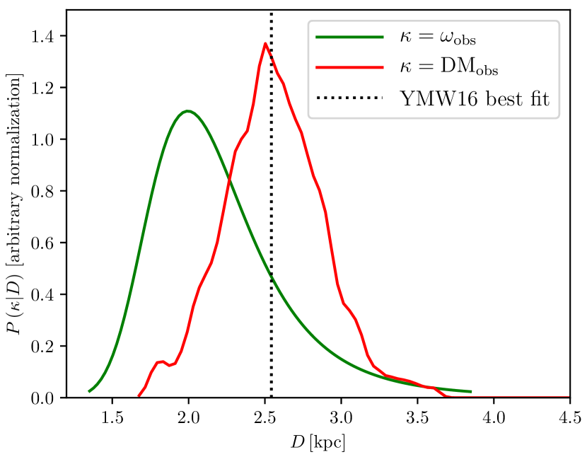
where $n_{e}$ is number density of electrons along the line-of-sight. Whereas the DM for each source is well constrained, $n_{e}(l)$ is a source of large uncertainties for individual sources (Lorimer, 2001) and sometimes the cause of systematic biases (Yao et al., 2017). To date there are three main models for $n_{e}$: TC93 (Taylor & Cordes, 1993), NE2001 (Cordes & Lazio, 2002, used by the majority of past MSP luminosity function analyses), and the recent YMW16 (Yao et al., 2017). Yao et al. (2017) showed that the YMW16 model was less affected by the large errors which typically entered the NE2001 model, particularly at high galactic latitudes, the regime in which NE2001 was shown to have large systematic biases (Roberts, 2011). We assume the YMW16 model as a description of the electron density. The YMW16 model contains 35 free parameters describing a variety of galactic components contributing to the total electron density, for example the scale height of the thick disk. In principle these could all affect the distance calculated to a given source. For each pulsar a PDF is generated for the observed dispersion measure as a function of true distance. We adopt a conservative approach by sampling from all variable parameters and calculating the dispersion measure for each pulsar given a true distance to the source. Gaussian distributions around each parameter are assumed with the central values and $1\sigma$ errors as provided in Table 2 of Yao et al. (2017). We sample $10^{5}$ combinations of parameters and true distances for each pulsar and create a PDF by binning the data in a histogram. An example is provided in Fig. 1. Using this method, we found that the PDF always peaks extremely close to the best fit value from the YMW16 model but there can be quite significant spread, even though most of the parameters in the YMW16 model are quite well constrained.

All code to reproduce the DM-based probability-distribution functions for either the dispersion measure or the distance to an individual pulsar are publicly available at https://github.com/tedwards2412/MSPDist. We provide a python wrapper for the YMW16 electron-density model (Yao et al., 2017) and accompanying code to calculate distance uncertainties.

Figure 1: Probability distribution for the measured parallax and dispersion measure of J1600-3053 given the true distance of the source. PDFs have an arbitrary normalization. The black-dotted line shows the distance corresponding the observed dispersion measure and the best-fit parameters of the YMW model. Varying the parameters of the YMW16 model yields the distribution shown in red. The green line corresponds to the PDF for the parallax.

2.3 Pulsar sample

2.3.1 $\gamma$-ray detected pulsars

In our benchmark analysis we exclusively use the $\gamma$-ray detected MSPs not associated with a globular cluster. All sources have spin periods $\leq 30\mathrm{\,ms}$. Our sample contains 96 sources with confirmed $\gamma$-ray pulsations (see Tab. 4). The source list is compiled using the second pulsar catalog (2PC) (Abdo et al., 2013) and the public list of Fermi-LAT detected $\gamma$-ray pulsars as was available on May 14 2018 . Unless specified otherwise, fluxes are taken from the third Fermi-LAT source catalog (3FGL, Acero et al., 2015). When a pulsar is not present in the 3FGL we also look for fluxes in the second Fermi-LAT source catalog (2FGL, Nolan et al., 2012) and the FL8Y. Similarly, parallax and dispersion measures are obtained from the ATNF catalog (Manchester et al., 2005).

2.3.2 Unassociated sources

The 3FGL contains $3033$ objects with roughly a third still unassociated to a particular source type. Follow-up radio observations of many of the unassociated sources have shown that there could be a large population of pulsars still remaining to be found within the 3FGL. If only a small proportion turn out to be MSPs this population will still tend to dominate the overall data set. We therefore must attempt to take this population into account and see how it could systematically affect our results. We capture the possible effects of the unassociated sources by presenting three scenarios. First, we perform our analysis using only the 96 $\gamma$-ray detected sources. In addition, we perform the same analysis using only the 39 MSPs present in the 2PC. Finally, we combine the 96 $\gamma$-ray detected sources with 69 sources without $\gamma$-ray detected pulsations based on the results from Saz Parkinson et al. (2016). Although some of these 69 sources have unconfirmed associations, we will refer to this sample as unassociated sources for conciseness. These can be found in Table 4 under ’other sources’.

Saz Parkinson et al. (2016) performed a classification analysis of the 3FGL using a variety of Machine Learning tools, the most accurate being Random Forest which achieved $>90\%$ correct associations when trained on $70\%$ of the sample and tested on the remaining $30\%$. For the construction of our unassociated sample, we select all 3FGL unassociated sources and source candidates of any given class that have not been confirmed. We require that each source is classified as a pulsar by either the logistic regression or Random Forest analysis of Saz Parkinson et al. (2016) with over 50% probability. Moreover, we require the same classifier to classify the candidate as an MSP rather than a young pulsar. Finally, we require a detection significance in the 3FGL or FL8Y of $\geq 10\sigma$, similar to the list in Table 6 of Saz Parkinson et al. (2016) to optimize the chances of the classification being correct. We note a few of the prime candidates in this table have since been discovered as $\gamma$-ray MSPs, including the two recent detections by Clark et al. (2018).

2.4 Parameter scan

We efficiently scan the parameter space using the Bayesian nested sampling package MultiNest (Feroz et al., 2009; Buchner et al., 2014). For the low-dimensional problems at hand, MultiNest is accurate and requires a computationally feasible number of likelihood calculations to accurately map the posterior distribution. In addition it is able to handle multi-modal distributions and degeneracies in the parameter space, the latter being a problem we are likely to encounter when considering particular configurations of luminosity functions, such as PL with a maximum luminosity cut-off. The results presented in Sec. 3 use nlive$\,=500$.

For each model the Bayesian evidence is computed (e.g.  Trotta, 2008)

$$\mathcal{Z}=P\left(\mathcal{D}\right)=\int\mathcal{L}\left(\mathbf{\Theta}\right)\mathcal{\pi}(\mathbf{\Theta})d\mathbf{\Theta},$$ (14)

where $\mathcal{\pi}(\Theta)$ is the prior on each parameter. The Bayes factor is then defined as

$$\begin{split}B_{12}&\equiv\frac{P\left(H_{2}\right|\mathcal{D})}{P\left(H_{1}\right|\mathcal{D})}=\frac{\mathcal{Z}_{2}P(H_{2})}{\mathcal{Z}_{1}P(H_{1})},\end{split}$$ (15)

with $H_{1,2}$ denoting the different models (Trotta, 2008). We choose equal priors for different models, $P(H_{2})/P(H_{1})=1$. Since our models are not nested hypotheses, Bayesian model selection, which does not require this assumption, provides a straightforward comparison of our models. We note that, in contrast to Frequentist analyses, it is here relevant to properly normalize the likelihood functions in order to make the evidence and the Bayes factor informative. The expressions in Eq. 1 and Eq. 4 ensure this.

3 Results

3.1 Model comparison

For each of the three data sets ($\gamma$-ray detected MSPs, MSPs plus MSP candidates from Saz Parkinson et al. (2016) and the 2PC MSPs) we compare multiple models, each characterized by their luminosity function, spatial profile and whether or not we included a bulge population.

In order to interpret the results we use Bayesian model comparison following Kass & Raftery (1995). We compute $2\ln B_{12}$ from Eq. 15 always comparing against a benchmark model ($H_{2}$: BPL, Lorimer). If $2\ln B_{12}\in[0,2]$ there is no preference for $H_{2}$ over $H_{1}$. $2\ln B_{12}>10$ represents strong preference for $H_{2}$. Contrarily, $2\ln B_{12}<0$ indicates $H_{1}$ is preferred over $H_{2}$.

Model	$\ln\mathcal{Z}$	$2\ln B_{12}$
$\gamma$-ray detected pulsars
BPL, Lorimer	2042.0	0.0
BPL, Lorimer, bulge	2041.6	0.8
LN, Lorimer	2040.0	4.0
LN, Lorimer, bulge	2040.0	4.0
PL exp. cutoff, Lorimer	2036.6	10.8
BPL, gaussian	2024.0	36.0
BPL, gaussian, bulge	2023.7	36.6
LN, gaussian	2021.8	40.4
LN, gaussian, bulge	2021.2	41.6
PL, Lorimer	2017.6	48.8
All sources
BPL, Lorimer	3889.6	0.0
BPL, Lorimer, bulge	3889.6	0.0
LN, Lorimer	3888.3	2.6
BPL, gaussian	3875.9	27.4
LN, gaussian	3874.4	30.4
2PC
BPL, Lorimer	789.0	0.0
LN, Lorimer	787.9	2.2
BPL, gaussian	780.0	18.0
LN, gaussian	778.8	20.4

Table 2: Model comparison for the three different datasets analyzed. Each model is characterized by the luminosity function, spatial profile and whether or not we included a bulge population. We show the log of the Bayesian evidence ($\ln\mathcal{Z}$) for each model and the Bayes factor ($B_{12}=2\ln\mathcal{Z}_{2}/\mathcal{Z}_{1}$) with respect to the best-fitting model without bulge (Kass & Raftery, 1995).

The results for the various MultiNest scans performed are shown in Tab. 2. Each dataset is shown separately and models are ordered by decreasing $\mathcal{Z}$. Our default dataset ($\gamma$-ray detected pulsars only) shows that a single power-law parameterization of the luminosity function, regardless of whether it has a hard or super-exponential cutoff, is greatly disfavored. No strong preference is present for either a log-normal or broken power-law parameterization, although the latter performs slightly better. Concerning the spatial profile, the Lorimer disk is strongly preferred over the radial Gaussian profile. No bulge component is required by the data. A small point of caution, in a few cases the evidence of models including the bulge is smaller than of identical models without a bulge component. However, the likelihood for the models including the bulge is higher than that of those where it is not included, which is expected when including additional degrees of freedom. The fact that the evidence goes down with the addition of a new component means that the model without the additional component suffices to describe the data. Given these results, we will henceforth consider the Lorimer disk with a BPL luminosity function and no bulge as our benchmark model and show results for this run. Additional results can be found in Appendix D.

3.2 Parameters

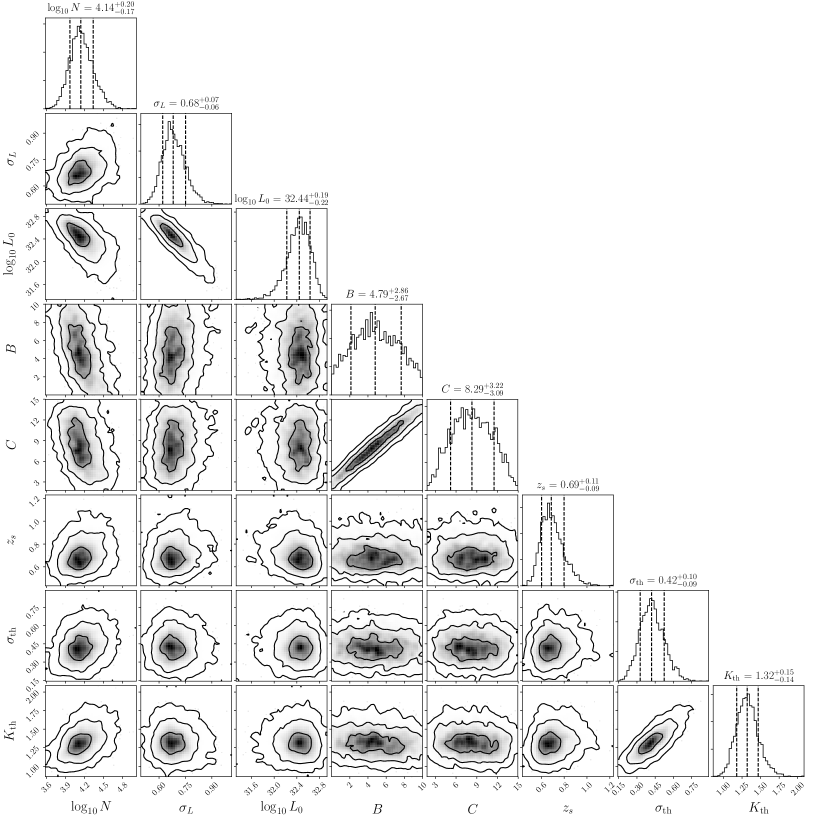
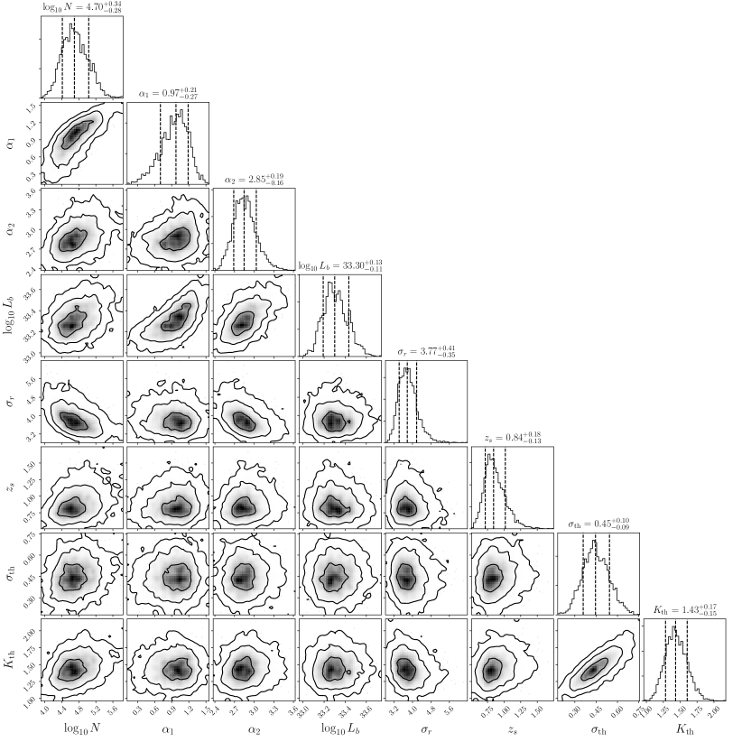
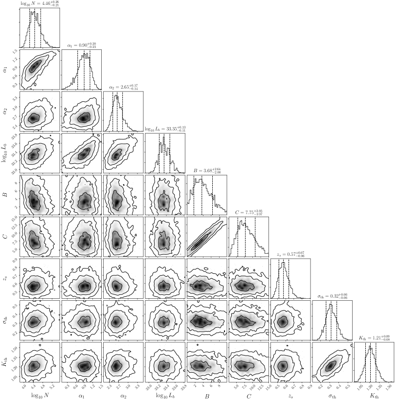
In Fig. 2 we show a corner plot for the parameters of our benchmark model. Contours in the two-dimensional histograms are $1,2$ and $3\sigma$. Dashed-lines in the one-dimensional posterior represent $16,50$ and $84\%$ quantiles. The best fit parameters for our benchmark model and for the log-normal luminosity function with a Lorimer disk are given in Tab. 3.2. Corner plots for other representative models in Tab. 2 are presented in Appendix D.

Figure 2: Corner plot for the parameters of our benchmark model. Contours in the two-dimensional histogram are $1,2$ and $3\sigma$. Dashed-lines in the one-dimensional posterior show the $16,50$ and $84\%$ quantiles. Values above each posterior represent the $50\%$ quantile with $1\sigma$ errors.

Table 3: Best-fit parameters and characteristics for the populations with a broken power-law and log-normal luminosity function and Lorimer-disk spatial profile. Luminosities and fluxes are in the range $0.1-100\mathrm{\,GeV}$.

Parameter	broken power-law	log-normal
Luminosity function
$\log_{10}L_{\mathrm{min}}$	$30$	$30$
$\log_{10}L_{\mathrm{max}}$	$37$	$37$
$\alpha_{1}$	$0.97$	-
$\alpha_{2}$	$2.60$	-
$\log_{10}{L_{b}}$	$33.24$	-
$\log_{10}{L_{0}}$	-	$32.61$
$\sigma_{L}$	-	$0.63$
Spatial profile
$B$	$3.91$	$2.75$
$C$	$7.54$	$5.94$
$z_{s}$	$0.76$	$0.63$
Detection sensitivity
$\sigma_{\mathrm{th}}$	$0.41$	$0.45$
$K_{\mathrm{th}}$	$1.35$	$1.33$
Other characteristics
$\log_{10}{N}$	$4.38$	$4.12$
$\left<L\right>\mathrm{\,[erg\,s^{-1}]}$	$6.2\times 10^{32}$	$1.1\times 10^{33}$
$L_{\mathrm{tot}}\mathrm{\,[erg\,s^{-1}]}$	$1.5\times 10^{37}$	$1.5\times 10^{37}$
$F_{\mathrm{tot}}\mathrm{\,[erg\,cm^{-2}\,s^{-1}]}$	$4.7\times 10^{-9}$	$4.8\times 10^{-9}$
Expected bulge detections	$4.5$	$2.9$

The total number of sources with $L\geq L_{\mathrm{min}}$ is $\sim 2\times 10^{4}$ for our best-fit model. However, it could be as small as $\sim 10^{4}$ or as large as $\sim 10^{5}$. Unlike previous claims (Grégoire & Knödlseder, 2013), we find the $\gamma$-ray MSP population to be compatible with the the expected number of MSPs from population studies using radio pulsars (Cordes & Chernoff, 1997; Lyne et al., 1998; Levin et al., 2013).

Luminosity function

In Fig. 3 we show the luminosity function. The blue solid line displays the total luminosity function, whereas the dashed line shows the luminosity function with the detection efficiency folded in. The grey shaded area corresponds to one or fewer sources at this luminosity.

Orange errorbars show the expectation values derived from the data. Uncertainties in the flux and distance to individual pulsars have been taken into account (see Appendix C.2). Upper limits correspond to an expectation of fewer than one source in the particular bin. In addition, we show the cumulative distribution of the luminosity function in Fig. 4. The data point and errorbars show the median and the 95% containment interval.

Figure 3: Luminosity function ($0.1-100\mathrm{\,GeV}$) of our benchmark model. The blue solid line shows the total luminosity function, whereas the dashed line only shows the expected sources. Orange errorbars are the expectations-values from the data where distance and flux uncertainties have been taken into account (for more details see Appendix C.2). The grey-shaded area corresponds to one or fewer sources.

Figure 4: Similar to Fig. 3, but showing the cumulative distribution. Distance and flux uncertainties for individual pulsars are included in the errorbars, which show the median and 95% containment interval.

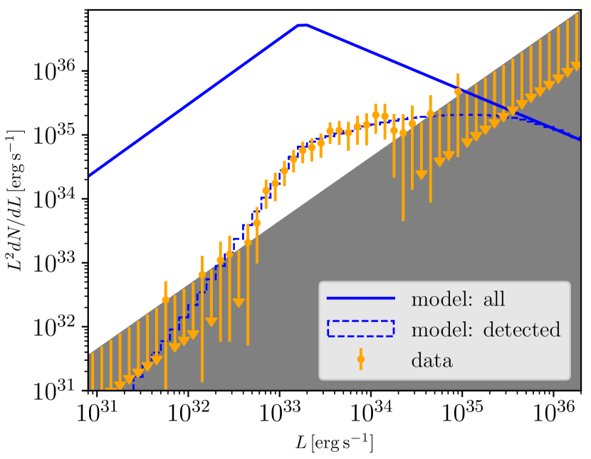
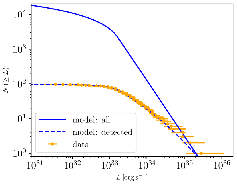
At $\sim 2\times 10^{33}\mathrm{\,erg\,s^{-1}}$ there is a clear turnover. Due to the hard slope at low luminosities ($\alpha_{1}=1.0$) and soft slope at high luminosities ($\alpha_{2}=2.6$) the total flux is dominated by sources somewhat below the break luminosity. There is no indication of any MSPs brighter than $\mathrm{few}\times 10^{35}\mathrm{\,erg\,s^{-1}}$ or dimmer than $\sim 10^{32}\mathrm{\,erg\,s^{-1}}$. This parameterization broadly agrees with the results from Winter et al. (2016).

Spatial profile

Spatial parameters are not very well constrained. The scale height of the disk is $\sim 0.7{\rm\,kpc}$ but has an uncertainty of a factor $\sim 1.5$, in broad agreement with earlier works (e.g.  Story et al., 2007; Levin et al., 2013; Calore et al., 2014; Hooper & Mohlabeng, 2016; Ploeg et al., 2017). The radial parameters of the Lorimer profile are consistent with the distribution derived for the full radio pulsar population (Lorimer, 2003; Lorimer et al., 2006) and with expectations for the MSP population (Lorimer et al., 2015). For the Gaussian profile (see Appendix D), the dispersion is $\sigma_{r}\sim 4\mathrm{\,kpc}$, but is again uncertain by $\sim 25\%$. This result is consistent with the expectations for an old pulsar population Faucher-Giguere & Loeb (2010). Our results for the spatial profile are also in agreement with other analyses of $\gamma$-ray MSPs (Hooper & Mohlabeng, 2016; Ploeg et al., 2017).

Figure 5: Latitude distribution of MSPs. Blue is the expected distribution. Orange data points show the observed distribution.

Figure 6: Same as Fig. 5 but for longitude.

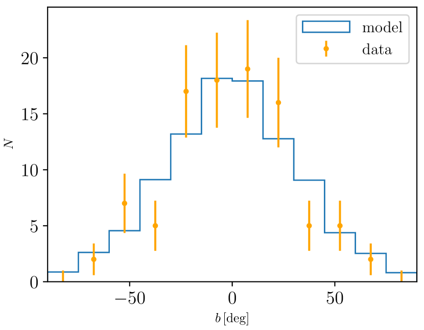
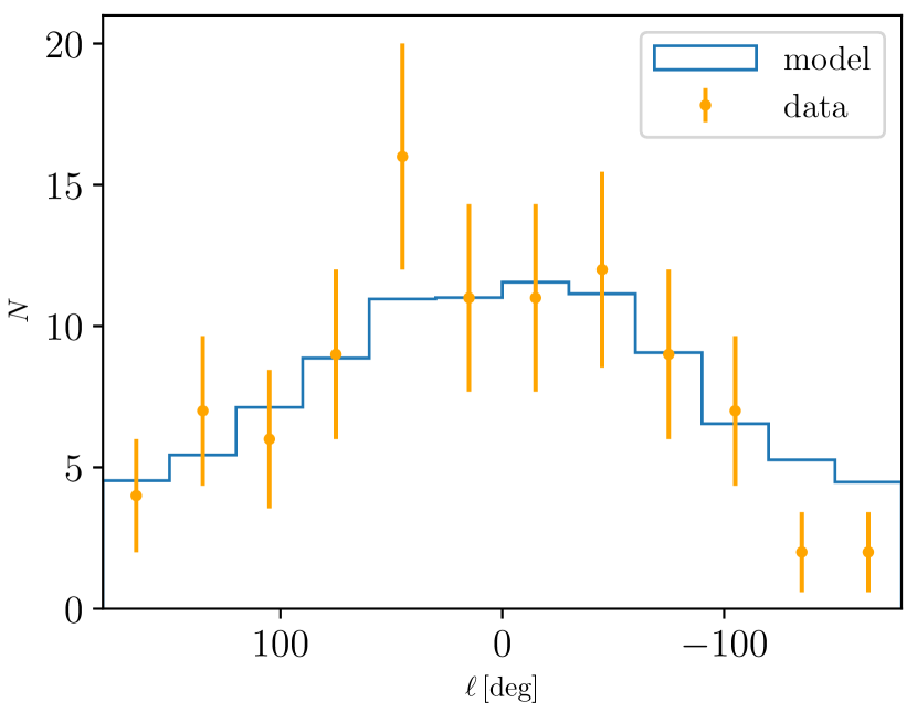
In Figs. 5 and 6 we show the expected (blue) and observed (orange) latitude and longitude distribution of $\gamma$-ray detected MSPs.

Detection sensitivity

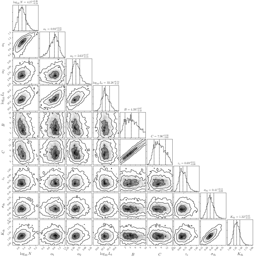
In principle, the parameters $\left\{K_{\mathrm{th}},\sigma_{\mathrm{th}}\right\}$ are nuisance parameters. The positive value of $K_{\mathrm{th}}$ indicates that our detection sensitivity is poorer than the sensitivity map we use (Abdo et al., 2013). However, this is not unexpected since Abdo et al. (2013) derived their map assuming $\gamma$-ray sources with a pulsar spectrum, but did not require pulsations to be detected. We find, for the different datasets, i.e. 2PC, $\gamma$-ray detected pulsars, and including not-yet-identified sources, the values $\left\{K_{\mathrm{th}},\sigma_{\mathrm{th}}\right\}=\left\{2.05,0.64\right\},\left\{1.35,0.41\right\}$, and $\left\{1.19,0.30\right\}$ respectively. Therefore, we see that the detection sensitivity improves with a larger sample which is expected since a larger sample implies either increased exposure, such as when going from the 2PC to the full $\gamma$-ray detected pulsars sample, or a more lenient detection criteria, such as when we include unassociated sources.

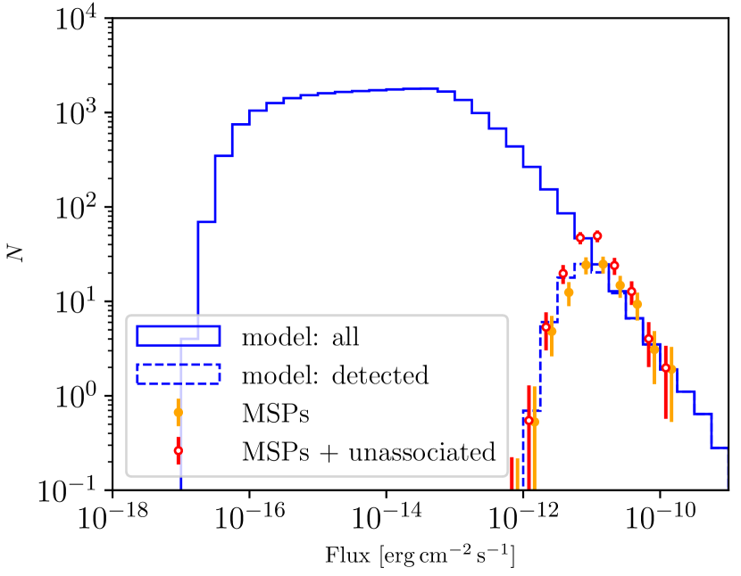
For completeness, we show the flux distribution in Fig. 7. The blue solid line is the total population, whereas the blue dashed line takes into account the detection threshold. As can be seen our analysis suggests the MSP population is flux complete down to $F\gtrsim 10^{-11}\mathrm{\,erg\,cm^{-2}\,s^{-2}}$.

Figure 7: Flux distribution for our benchmark model. The blue solid line is the total MSP population. The dashed blue line takes into account the detection threshold. Orange errorbars are the data including all $\gamma$-ray detected pulsars. Red-open errorbars also include the 69 unassociated sources. Note that the blue-dashed line corresponds to the detection sensitivity derived using only the $\gamma$-ray detected pulsars.

3.3 Total Luminosity and Flux

Given the number of sources and luminosity function we can determine the total luminosity. Since the broken-power law peaks at luminosities of $\sim 10^{33}\mathrm{\,erg\,s^{-1}}$ and has a hard (soft) slope at low (high) luminosities, the total luminosity is fairly insensitive to $L_{\mathrm{min}}$ and $L_{\mathrm{max}}$. The same holds for the log-normal distribution. We find a total luminosity $L_{\mathrm{tot}}=1.5\times 10^{37}\mathrm{\,erg\,s^{-1}}$ and a total flux of $4.7\times 10^{-9}\mathrm{\,erg\,cm^{-2}\,s^{-1}}$. These numbers are uncertain by about a factor $\sim 2$. Given a Milky-Way stellar-disk mass of $5.17\times 10^{10}\mathrm{\,M_{\odot}}$ (Licquia & Newman, 2015) we find that luminosity-per-stellar-mass for the Milky-Way disk is $2.9\times 10^{26}\mathrm{\,erg\,s^{-1}\,M_{\odot}^{-1}}$.

4 Discussion

4.1 Unassociated sources

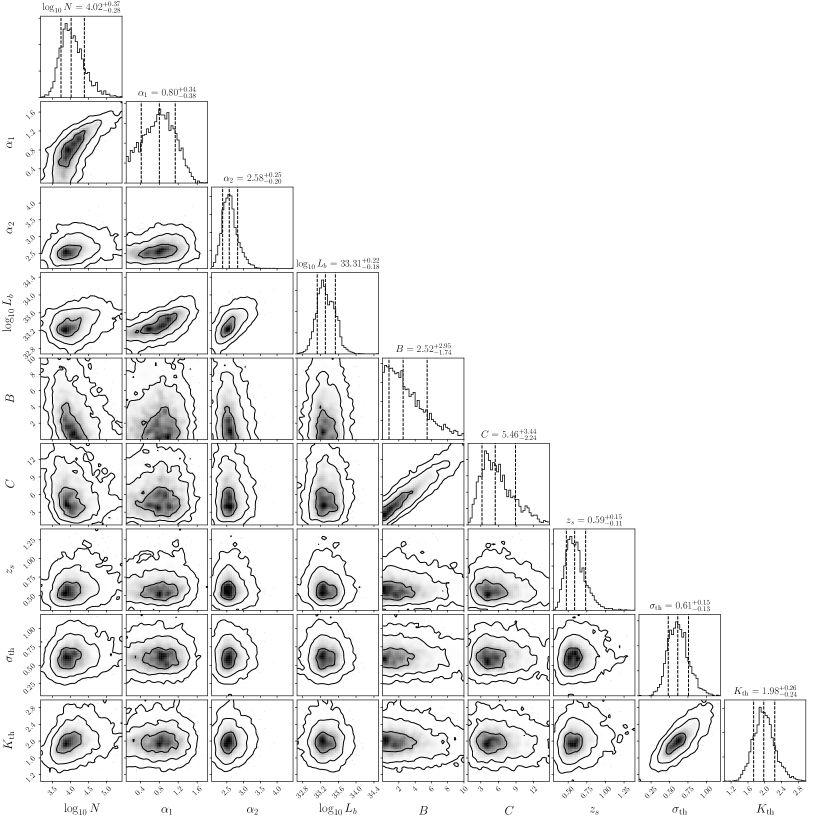
Our default analysis includes 96 $\gamma$-ray detected MSPs. In addition, we performed analyses using only the 39 MSPs from the 2PC (Abdo et al., 2013) and including an additional 69 unassociated sources with selection criteria based on the results of Saz Parkinson et al. (2016). We find consistent results between the three analyses. In particular, as can be seen in Tab. 2, in all cases we find that there is no clear preference for either a broken-power law or a log-normal luminosity-function parameterization. On the other hand, the Lorimer profile is always preferred over the Gaussian disk. Moreover, the inferred parameters agree within errors between different datasets, but get more tightly constrained by larger datasets (see Figs 2, 12 and 13).

This leads us to the somewhat surprising conclusion that for the purpose of our analysis there is no strong bias when including only $\gamma$-ray detected MSPs in the analysis. A priori this is not obvious, since all but one source have radio counterparts which could lead to a selection bias which cannot be efficiently accounted for in the detection sensitivity. Moreover, for all but one of the unassociated sources we do not have distance priors. This analysis however shows that we can derive consistent constraints whether or not distance information is included (also see Hooper & Mohlabeng (2016)).

In the future, it would be interesting to include a larger sample of likely pulsar candidates in order to constrain the luminosity function down to lower fluxes. In particular, without radio counterpart, it is difficult to confirm $\gamma$-ray pulsations in blind searches (Clark et al., 2018). One possibility would be an update of the work by Saz Parkinson et al. (2016) using a larger source catalog. In addition, Ajello et al. (2017) propose a potentially powerful technique which classifies unassociated sources as likely pulsar candidates and which uses a customized detection efficiency.

4.2 Implications for the Galactic Center Excess

We tested for the presence of a bulge MSP population by including an additional component in our analysis (Sect. 2), but find no evidence for the presence of such a population (Sect. 3). This analysis assumes that bulge MSPs follow the same luminosity function as disk MSPs. Using the same assumption and the observed GCE intensity we can also estimate how many MSPs from the bulge should have been detected. We use a GCE intensity of $2.3\times 10^{-9}\mathrm{\,erg\,cm^{-2}\,s^{-1}}$ (Bartels et al., 2017) and distance to the GCE of $R_{\odot}=8.5\mathrm{\,kpc}$ to normalize the bulge population. Using the best-fit detection efficiency and luminosity function of our benchmark model we estimate that $4.5$ sources should have been detected. Within the 95% containment interval of the full posterior the number of bulge MSP detections ranges from being fewer than one to more than a dozen. Using the dataset that includes unassociated sources, this number goes up to $5.5$. Similar numbers are obtained for the log-normal luminosity function. We therefore agree with Ploeg et al. (2017) that the MSP interpretation of the GCE is consistent with the luminosity function derived from MSPs in the Galactic disk.

We find that opposite conclusions are driven by the high-luminosity tail of the luminosity function. At the distance of the GC mostly sources with luminosities $\gtrsim 2\times 10^{34}\mathrm{\,erg\,s^{-1}}$ can be detected. Hooper & Mohlabeng (2016) find relatively more bright sources ($\geq 10^{34}\mathrm{\,erg\,s^{-1}}$), and thus a higher number of expected bulge detections, compared to this work and Ploeg et al. (2017). Similarly, the MSP population in globular clusters has about an order-of-magnitude higher mean luminosity than what we derive for the disk (Hooper & Linden, 2016). The treatment of the flux threshold only has a mild impact. Here and in Ploeg et al. (2017) both $K_{\mathrm{th}}$ and $\sigma_{\mathrm{th}}$ are left free in the fit. However, Hooper & Mohlabeng (2016) fix $\sigma_{\mathrm{th}}=0.9$, which is larger than our best-fit value. Although this leads to a larger acceptance of dim sources, the detection probabilities at $\gtrsim 3\times 10^{34}\mathrm{\,erg\,s^{-1}}$ are very similar.

It should be mentioned that all but one of the $\gamma$-ray detected MSPs have radio counterparts. It is notoriously difficult to detect MSPs in radio near the Galactic Center due to the large scatter broadening of pulsed emission (e.g.  Calore et al., 2016). Since we apply a detection threshold based on $\gamma$-ray flux this does not directly take into account the decreasing sensitivity of radio searches with increasing distance. Consequently, if bulge MSPs are present in our full sample it is not unlikely that they are all unassociated sources. In the near future, the radio sensitivity for searches of bulge MSPs should increase significantly, allowing for the detection of this component in radio (Calore et al., 2016).

If the GCE originates from MSPs in the disk we find a bulge-to-disk ($B/D$) luminosity (flux) ratio of $B/D\sim 1.3\,(0.5$). The ratio of luminosity-to-stellar mass in the bulge is $2.2\times 10^{27}\mathrm{\,erg\,s^{-1}\,M_{\odot}^{-1}}$ compared to $2.9\times 10^{26}\mathrm{\,erg\,s^{-1}\,M_{\odot}^{-1}}$ in the disk. Therefore, the bulge appears to host approximately eight times more MSPs per unit stellar mass than the disk, consistent with the results from Bartels et al. (2017).

4.3 Completeness

We discuss the completeness we obtain from our analysis, i.e. the number of detected sources over the total number of sources in the disk, and compare it to the results of Winter et al. (2016). Although Winter et al. (2016) find a comparable parameterization of the luminosity function, their normalization and therefore total luminosity is about a factor $7$ larger than what we find (Winter et al., 2016; Eckner et al., 2017). This difference can be ascribed to the fact that our analysis yields a larger completeness by about a factor $\sim 10$ at the peak of the luminosity function ($L\sim 10^{33}\mathrm{\,erg\,s^{-1}}$). It should be taken into account that we use a larger sample of MSPs, 96 versus 66 in Winter et al. (2016). Naively rescaling by this ratio still leaves a factor $\sim 7$ higher completeness.

We find the reason for the difference in completeness to be twofold. First, Winter et al. (2016) estimate completeness by performing a Monte-Carlo (MC) simulation. They randomly draw pulsars at a given luminosity and assign it a position by drawing from a Lorimer profile with $B=0$, $C=2.8$ and $z_{s}=0.6$ (Story et al., 2007; Grégoire & Knödlseder, 2013; Winter et al., 2016). In fact, $C$ and $z_{s}$ are themselves also drawn from log-normal distribution. This profile is consistent with our best-fit value at $\sim 2\sigma$. We compare the impact this has on the completeness by running a MC simulation drawing sources at different luminosities and assigning them spatial positions based on the distribution assumed in Winter et al. (2016) and our benchmark distribution. With the spatial profile from Winter et al. (2016) the MSPs are on average slightly further away compared to our benchmark spatial profile. Consequently, the flux received from each source is about a factor $\sim 2$ dimmer, which so happens to also result in a loss of completeness by a factor $\sim 2$. This is displayed Fig. 8 as the difference between the green and red lines with the same linestyle. Second, the detection threshold applied by Winter et al. (2016) is based on latitude dependent flux threshold in Fig. 17 from Abdo et al. (2013), whereas we use the map in Fig. 16 of that same work. In our MC simulation we also compare these two detection sensitivities. In Fig. 8 this is shown by the difference between the solid (our detection sensitivity) and dashed (sensitivity threshold from Winter et al. (2016)) lines of the same color. We find that our sensitivity function yields a larger completeness. Finally, we note that in our MC simulation the red solid line corresponds to our benchmark model and the green solid line to our reproduction of the completeness from Winter et al. (2016), with their spatial distribution and flux threshold. In the bottom panel we show the ratio of the red-solid line (our work) over the green-dashed line (our MC reproduction of Winter et al., 2016, which agrees very well).

Figure 8: Top panel: Comparison of completeness between this work (solid red line) and Winter et al. (2016) (black dotted line). The dark (light) grey band shows the 68% (95%) containment interval of the completeness obtained in this work. Color and line style indicate spatial distribution and flux threshold respectively. Red (green) use the spatial distribution from this work (Winter et al. (2016)). The solid (dashed) lines use the flux threshold from this work (Winter et al. (2016)). The green dashed line shows our reproduction of the MC simulation of Winter et al. (2016), using their spatial distribution and flux sensitivity. Bottom panel: ratio of the red-solid over the green-dashed line.

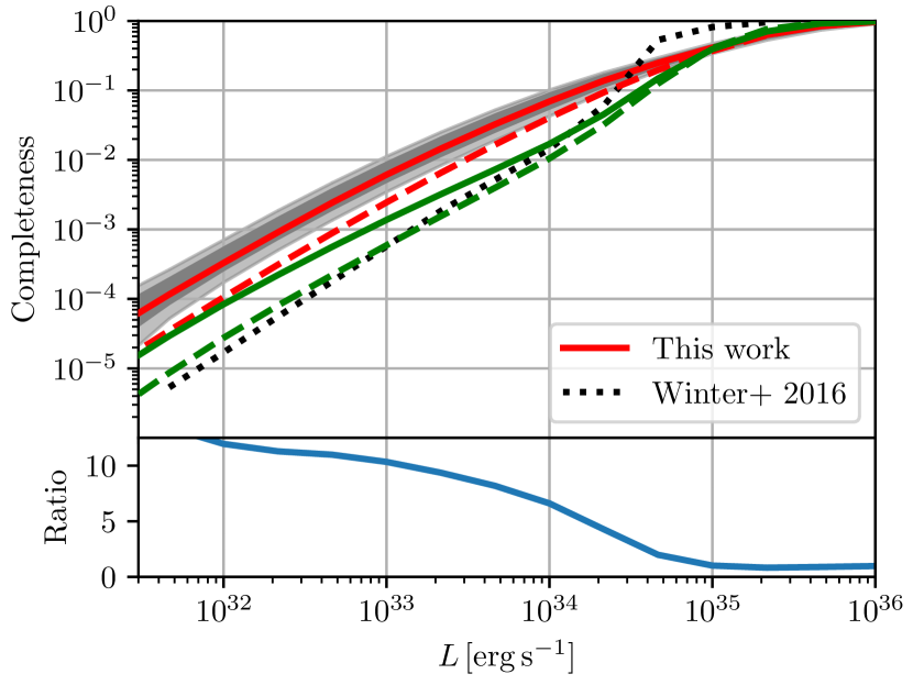
A merit of our analysis is that it is fully self-consistent in that we model the spatial-distribution, luminosity function and flux sensitivity simultaneously. Therefore, we consider the grey band in Fig. 8 to be the most trustworthy representation of the completeness. It shows the 68% and 95% containment interval of the completeness for our benchmark model. We construct it by sampling spatial and flux-sensitivity parameters from the full MultiNest posterior and consecutively running a MC simulation to estimate the completeness for each point.

The estimated completeness at the peak of the luminosity function has a large impact on the derived ratio of emission per unit stellar mass and therefore the expected unresolved flux. Any conclusions that relies directly on the completeness by estimating the luminosity of MSPs in a given environment by applying the luminosity-per-stellar mass from the disk is affected by this uncertainty. With our estimate of the completeness we expect MSPs from the disk to contribute $\mathcal{O}(1\%)$ to the total $\gamma$-ray flux from $1$–$10\mathrm{\,GeV}$, where the MSP spectrum is most pronounced (McCann, 2015). Moreover, studies of dwarf spheroidal galaxies (Winter et al., 2016), Andromeda (Eckner et al., 2017) and the Galactic Bulge (Macias et al., 2018; Bartels et al., 2017) are also affected by our estimated completeness.

5 Conclusion

We have performed a Bayesian-unbinned likelihood analysis and – for the first time in this context – done Bayesian model comparison in order to constrain the properties of the Galactic population of $\gamma$-ray MSPs, self-consistently taking into account various sources of uncertainties. We used a sample of $96$ $\gamma$-ray detected MSPs, but verified that our results remain similar under the inclusion of an additional $69$ well-motivated MSP candidates. In order to deal with distance uncertainties we developed a novel method to construct PDFs for the distance to individual pulsars and the distance proxies. We use the YMW16 electron-density model to construct a PDF for the dispersion measure given the true distance to a pulsar by sampling from the model its $35$ free parameters. We therefore take into account the uncertainties on the derived parameters within the electron density model (Yao et al., 2017). Distance and flux uncertainties were then marginalized over. The normalization and variance of the flux-detection threshold were treated as free parameters in our analysis. Results for different parameterizations of the luminosity function and spatial profile are compared by computing Bayes factors.

We find that a Lorimer-disk profile is preferred over a disk with a Gaussian radial profile, although the parameters are only loosely constrained. There is clear evidence for a turnover in the luminosity function, ruling out a single power-law parameterization (with hard or super-exponential cutoff). Instead, both a broken-power-law and a log-normal function provide good fits to the luminosity function.

Our analysis suggests the presence of $\sim 2\times 10^{4}$ MSPs in the Galactic disk. However, within uncertainties this number could be as large as $\sim 10^{5}$. These numbers are in agreement with the expected MSP population derived using radio catalogs (Cordes & Chernoff, 1997; Lyne et al., 1998; Levin et al., 2013).

Contrary to previous claims (Hooper et al., 2013; Cholis et al., 2015; Hooper & Mohlabeng, 2016), we find the MSP interpretation of the GCE to be fully compatible with the characteristics of the disk MSPs. Therefore, we agree with the findings of Yuan & Zhang (2014); Petrović et al. (2015); Ploeg et al. (2017). Our characterization of the luminosity function and detection sensitivity suggest that if the luminosity function of the bulge MSP population is identical to that of the disk MPS, and if 100% of the GCE is due to MSPs, only a handful of sources should have been detected from the bulge, whereas in the past larger numbers were suggested. We explicitly tested for the presence of a bulge component in our analysis, but find that we currently lack sensitivity to place interesting constraints on the bulge population of MSPs. In the future, an extension of the work by Saz Parkinson et al. (2016) or a dedicated analysis to characterize unassociated sources as likely pulsars (Ajello et al., 2017) can be potentially powerful methods to constrain the bulge population.

At the peak of the luminosity function we find a higher detection completeness than previous work (Winter et al., 2016). Consequently, our luminosity-per-stellar-mass ratio of $\sim 3\times 10^{26}\mathrm{\,erg\,s^{-1}\,M_{\odot}^{-1}}$ is significantly smaller than what has been derived in other works (Winter et al., 2016; Macias et al., 2018; Eckner et al., 2017). It should be mentioned that the completeness suffers from considerable uncertainties due to its dependence on the detection sensitivity, spatial profile and luminosity function.

The results presented in this work have direct implications for the detectability of a diffuse disk MSP component due to unresolved sources, their contribution to the isotropic $\gamma$-ray background (Faucher-Giguere & Loeb, 2010; Siegal-Gaskins et al., 2011; Calore et al., 2014), the bulge-to-disk ratio of MSPs (Macias et al., 2018; Bartels et al., 2017), the expected emission from dwarf galaxies (Winter et al., 2016), and the detectability of MSPs in external Galaxies such as M31 (Eckner et al., 2017).

Although the properties of the galactic disk MSP population are the main topic of this paper, the methods we describe can be applied directly to any population of astrophysical sources where unassociated sources are present and distances uncertainties are large, a situation commonly found in population analyses.

Appendix A Millisecond pulsar sample

In Table 4 we show the source list used in this work. The full list is available at http://github.com/tedwards2412/MSPDist. We separated the table in $\gamma$-ray detected pulsars and unassociated sources. For each source we give the position, $\gamma$-ray flux ($0.1-100\mathrm{\,GeV}$), dispersion measure and/or parallax if available. Finally, the catalogs in which the sources appear are given.

Table 4: Millisecond pulsar sample separated into $\gamma$-ray detected MSPs and MSP candidates from Saz Parkinson et al. (2016) (see text for details). The different columns provide respectively: the name of the source, Galactic longitude and latitude in degrees, $\gamma$-ray flux in the range $0.1-100\mathrm{\,GeV}$, the dispersion measure and/or parallax from that ATNF (Manchester et al., 2005) if available, and finally a reference to the relevant catalogs.

Name	$\ell$	$b$	Flux	DM	Parallax	Catalogs
	$\left[\mathrm{deg}\right]$	$\left[\mathrm{deg}\right]$	$\left[10^{-12}\mathrm{\,erg\,cm^{-2}\,s^{-1}}\right]$	$\left[\mathrm{cm^{-3}\,pc}\right]$	$\left[\mathrm{mas}\right]$
$\gamma$-ray pulsars (96)
J0023+0923	111.5	-52.9	$7.28\pm 0.81$	14.33	$0.93\pm 0.16$	1,2,3,4,5
J0030+0451	113.1	-57.6	$60.68\pm 1.51$	4.34	$3.08\pm 0.09$	1,2,3,4,5
J0034-0534	111.5	-68.1	$18.04\pm 1.02$	13.77	*	1,2,3,4,5
J0101-6422	301.2	-52.7	$12.45\pm 0.85$	11.93	*	1,2,3,4,5
J0102+4839	124.9	-14.2	$16.76\pm 1.39$	53.50	*	1,2,3,5
J0218+4232	139.5	-17.5	$48.14\pm 1.80$	61.25	$0.16\pm 0.09$	1,2,3,4,5
J0248+4230	144.9	-15.3	$5.21\pm 0.81$	48.2	*	2,4,5
J0251+26	153.9	-29.5	$6.87\pm 0.99$	20.00	*	2,3,4,5
J0308+74	131.7	14.2	$14.57\pm 0.79$	6.35	*	2,3,5
J0318+0253	178.4	-43.6	$5.71\pm 0.74$	26.	*	2,3,4,5
J0340+4130	153.8	-11.0	$22.24\pm 1.33$	49.59	$0.7\pm 0.5$	1,2,3,4,5
J0437-4715	253.4	-42.0	$17.87\pm 0.88$	2.64	$6.37\pm 0.09$	1,2,3,4,5
J0533+67	144.8	18.2	$9.57\pm 0.89$	57.40	*	2,3,5
J0605+37	174.2	8.0	$6.88\pm 0.95$	21.00	*	2,3,5
J0610-2100	227.7	-18.2	$11.48\pm 1.07$	60.67	*	1,2,3,4,5
J0613-0200	210.4	-9.3	$33.57\pm 1.64$	38.78	$0.93\pm 0.2$	1,2,3,4,5
J0614-3329	240.5	-21.8	$110.80\pm 2.36$	37.05	*	1,2,3,4,5
J0621+25	187.1	5.1	$11.04\pm 1.50$	83.60	*	2,3,4
J0737-3039A	245.2	-4.5	$4.00\pm 1.00$	48.92	*	5
J0740+6620	149.7	29.6	$4.77\pm 0.68$	14.96	$2.3\pm 0.7$	2,4,5
J0751+1807	202.8	21.1	$13.04\pm 0.97$	30.25	$0.82\pm 0.17$	1,2,3,4,5
J0931-1902	251.0	23.0	$3.00\pm 0.86$	41.49	$1.2\pm 0.9$	2,4,5
J0955-61	283.7	-5.7	$8.24\pm 1.27$	160.70	*	2,5
J1012-4235	274.2	11.2	$7.48\pm 1.12$	71.60	*	2,3,4,5
J1023+0038	243.4	45.8	$5.35\pm 0.97$	14.32	$0.731\pm 0.022$	3,4
J1024-0719	251.7	40.5	$3.58\pm 0.52$	6.48	$0.8\pm 0.3$	1,2,3,4,5
J1035-6720	290.4	-7.8	$25.94\pm 1.47$	84.16	*	2,3,4,5
J1036-8317	298.9	-21.5	$5.78\pm 0.95$	27.00	*	2,4,5
J1124-3653	284.1	22.8	$13.16\pm 1.09$	44.90	*	1,2,3,5
J1125-5825	291.8	2.6	$14.51\pm 2.66$	124.79	*	1,2,3,4,5
J1137+7528	129.1	40.8	$2.28\pm 0.59$	29.1702	*	2,4,5
J1142+0119	267.6	59.4	$6.24\pm 0.82$	19.20	*	2,3,5
J1207-5050	295.9	11.4	$7.89\pm 1.16$	50.60	*	2,3,4,5
J1227-4853	299.0	13.8	$41.36\pm 1.67$	43.42	*	2,3,4,5
J1231-1411	295.5	48.4	$102.86\pm 2.12$	8.09	*	1,2,3,4,5
J1301+0833	310.8	71.3	$10.63\pm 0.97$	13.20	*	2,3,4,5
J1302-32	305.6	29.8	$11.30\pm 1.13$	26.20	*	2,3,5
J1311-3430	307.7	28.2	$64.69\pm 1.89$	37.84	*	2,3,4,5
J1312+0051	314.9	63.2	$16.50\pm 1.10$	15.30	*	2,3,5
J1431-4715	320.1	12.3	$6.41\pm 0.95$	59.35	*	4,5
J1446-4701	322.5	11.4	$12.55\pm 1.30$	55.83	*	1,2,3,4,5
J1455-3330	330.8	22.5	$2.15\pm 0.50$	13.57	$0.99\pm 0.22$	4,5
J1513-2550	338.8	27.0	$7.03\pm 0.98$	46.86	*	2,3,4,5
J1514-4946	325.2	6.8	$42.81\pm 2.12$	31.05	*	1,2,3,4,5
J1536-4948	328.2	4.8	$87.43\pm 3.05$	38.00	*	2,3,5
J1543-5149	327.9	2.7	$21.83\pm 2.60$	50.93	*	2,4,5
J1544+4937	79.2	50.2	$3.58\pm 0.64$	23.23	*	2,4,5
J1552+5437	85.6	47.2	$4.53\pm 0.64$	22.90	*	2,4,5
J1600-3053	344.1	16.5	$6.16\pm 1.07$	52.33	$0.5\pm 0.08$	1,2,3,4,5
J1614-2230	352.6	20.2	$23.37\pm 1.49$	34.92	$1.5\pm 0.1$	1,2,3,4,5
J1622-0315	10.8	30.7	$10.15\pm 1.28$	21.4	*	2,3,4,5
J1628-3205	347.4	11.5	$12.12\pm 1.48$	42.10	*	2,3,4,5
J1630+37	60.2	43.3	$6.86\pm 1.01$	14.10	*	2,3,5
J1640+2224	41.0	38.3	$2.59\pm 0.45$	18.46	$0.66\pm 0.07$	4,5
J1658-5324	334.9	-6.6	$20.32\pm 1.99$	30.81	*	1,2,3,4,5
J1713+0747	28.8	25.2	$9.41\pm 1.25$	15.92	$0.81\pm 0.03$	1,2,3,4,5
J1730-2304	3.2	6.0	$12.97\pm 2.38$	9.62	$1.19\pm 0.27$	4,5
J1732-5049	340.0	-9.4	$8.52\pm 1.34$	56.84	*	2,4,5
J1741+1351	37.9	21.6	$5.68\pm 1.06$	24.20	$0.56\pm 0.13$	1,2,3,4,5
J1744-1134	14.8	9.2	$39.16\pm 2.18$	3.14	$2.53\pm 0.07$	1,2,3,4,5
J1744-7619	317.1	-22.5	$22.50\pm 1.31$	*	*	2,3,4,5
J1745+1017	34.9	19.3	$10.56\pm 1.48$	23.97	*	2,3,4,5
J1747-4036	350.2	-6.4	$15.97\pm 1.79$	152.96	*	1,2,3,4,5
J1805+06	33.4	13.0	$5.51\pm 0.99$	65.00	*	2,3,4,5
J1810+1744	44.6	16.8	$22.38\pm 1.37$	39.70	*	1,2,3,4,5
J1811-2405	6.9	-2.5	$21.79\pm 4.30$	60.60	*	2,4
J1816+4510	72.9	24.8	$12.13\pm 0.93$	38.89	*	2,3,4,5
J1832-0836	23.0	0.2	$15.27\pm 2.99$	28.19	*	4,5
J1843-1113	22.0	-3.4	$19.81\pm 2.80$	59.96	$0.69\pm 0.33$	2,4,5
J1855-1436	20.4	-7.6	$7.85\pm 1.00$	109.2	*	4,5
J1858-2216	13.6	-11.4	$8.33\pm 1.09$	26.60	*	1,2,3,5
J1902-5105	345.6	-22.4	$21.47\pm 1.16$	36.25	*	1,2,3,4,5
J1902-70	324.4	-26.5	$12.28\pm 0.99$	19.50	*	2,3,5
J1909+21	53.7	5.8	$7.01\pm 1.10$	62.00	*	4,5
J1921+0137	37.8	-5.9	$15.92\pm 1.92$	104.9	*	2,3,4,5
J1939+2134	57.5	-0.3	$9.18\pm 3.32$	71.02	$0.22\pm 0.08$	1,4,5
J1946-5403	343.9	-29.6	$11.29\pm 0.92$	23.70	*	2,3,4,5
J1959+2048	59.2	-4.7	$17.91\pm 1.54$	29.12	*	1,2,3,4,5
J2017+0603	48.6	-16.0	$34.97\pm 1.69$	23.92	$0.4\pm 0.3$	1,2,3,4,5
J2017-1614	27.3	-26.2	$10.40\pm 1.20$	25.4380	*	2,3,4,5
J2042+0246	49.0	-23.0	$3.61\pm 0.55$	9.2694	*	2,4,5
J2043+1711	61.9	-15.3	$30.22\pm 1.41$	20.76	$0.64\pm 0.08$	1,2,3,4,5
J2047+1053	57.1	-19.6	$3.56\pm 0.58$	34.60	*	1,2,3,5
J2051-0827	39.2	-30.5	$3.18\pm 0.52$	20.73	*	1,2,4,5
J2052+1218	59.1	-20.0	$6.53\pm 1.04$	42.00	*	2,4,5
J2124-3358	10.9	-45.4	$39.40\pm 1.39$	4.60	$2.4\pm 0.4$	1,2,3,4,5
J2129-0429	48.9	-36.9	$10.50\pm 1.06$	16.90	*	2,3,4,5
J2205+6015	103.7	3.8	$7.50\pm 1.52$	157.6	*	4,5
J2214+3000	86.9	-21.7	$33.00\pm 1.24$	22.55	$2.3\pm 0.7$	1,2,3,4,5
J2215+5135	99.9	-4.2	$13.75\pm 1.14$	69.20	*	1,2,3,4,5
J2234+0944	76.3	-40.4	$8.28\pm 1.01$	17.8	$1.3\pm 0.5$	2,3,4,5
J2241-5236	337.4	-54.9	$30.97\pm 1.22$	11.41	*	1,2,3,4,5
J2256-1024	59.2	-58.2	$7.66\pm 0.78$	13.80	*	2,3,4,5
J2302+4442	103.4	-14.0	$38.10\pm 1.40$	13.73	*	1,2,3,4,5
J2310-0555	69.7	-57.9	$3.48\pm 0.56$	15.5139	*	2,4,5
J2339-0533	81.3	-62.5	$30.06\pm 1.39$	8.72	*	2,3,4,5
other sources (69)
J0039.3+6256	121.6	0.1	$9.11\pm 1.14$	*	*	2,3,4
J0212.1+5320	134.9	-7.6	$17.14\pm 1.56$	*	*	2,3,4
J0238.0+5237	138.8	-6.9	$11.60\pm 1.21$	*	*	2,3,4
J0312.1-0921	191.5	-52.4	$5.23\pm 0.84$	*	*	2,3,4
J0336.1+7500	133.1	15.5	$9.97\pm 1.04$	*	*	2,3,4
J0401.4+2109	171.4	-23.3	$6.27\pm 1.09$	*	*	3,4
J0523.3-2528	228.2	-29.8	$19.91\pm 1.24$	*	*	2,3,4
J0542.5-0907c	213.4	-19.4	$13.64\pm 1.81$	*	*	3,4
J0545.6+6019	152.5	15.7	$7.87\pm 0.95$	*	*	2,3,4
J0737.2-3233	246.8	-5.5	$13.83\pm 1.52$	*	*	2,3,4
J0744.1-2523	241.3	-0.7	$23.86\pm 1.78$	*	*	2,3,4
J0744.8-4028	254.6	-8.0	$9.40\pm 1.36$	*	*	3,4
J0758.6-1451	234.0	7.6	$7.30\pm 1.06$	*	*	2,3,4
J0802.3-5610	269.9	-13.2	$13.01\pm 1.18$	*	*	2,3,4
J0826.3-5056	267.4	-7.4	$10.66\pm 1.59$	*	*	3,4
J0838.8-2829	250.6	7.8	$12.74\pm 1.20$	*	*	2,3,4
J0933.9-6232	282.2	-7.9	$12.27\pm 1.06$	*	*	2,3,4
J0953.7-1510	251.9	29.6	$5.85\pm 0.71$	*	*	2,3,4
J0954.8-3948	269.8	11.5	$18.29\pm 1.23$	*	*	2,3,4
J0957.6+5523	158.6	47.9	$95.86\pm 2.73$	*	*	2,3,4
J1119.9-2204	276.5	36.1	$16.85\pm 1.03$	*	*	2,3,4
J1136.1-7411	297.8	-12.1	$11.18\pm 1.18$	*	*	2,3,4
J1207.6-4537	295.0	16.6	$4.17\pm 0.93$	*	*	3,4
J1208.0-6901	299.0	-6.5	$7.50\pm 1.25$	*	*	3,4
J1225.9+2953	185.2	83.8	$8.70\pm 0.97$	*	*	2,3
J1306.4-6043	304.8	2.1	$35.12\pm 2.50$	*	*	2,3,4
J1325.2-5411	307.9	8.4	$10.75\pm 1.65$	*	*	2,3,4
J1329.8-6109	307.6	1.4	$16.47\pm 2.39$	*	*	2,3,4
J1400.2-2413	322.4	36.0	$5.82\pm 0.99$	*	*	2,3,4
J1400.5-1437	326.9	45.0	$9.36\pm 1.09$	4.93	$3.6\pm 1.1$	2,3,4
J1412.3-6635	310.9	-5.0	$8.21\pm 1.46$	*	*	3,4
J1458.7-2120	338.6	32.6	$7.05\pm 1.05$	*	*	2,3,4
J1539.2-3324	338.8	17.5	$11.56\pm 1.03$	*	*	2,3,4
J1544.6-1125	356.2	33.0	$13.54\pm 1.40$	*	*	2,3,4
J1600.3-5810	325.8	-3.9	$5.50\pm 1.40$	*	*	3,4
J1616.8-5343	330.5	-2.2	$26.48\pm 2.62$	*	*	2,3,4
J1624.2-3957	341.1	6.6	$13.09\pm 2.53$	*	*	3,4
J1625.1-0021	13.9	31.8	$18.38\pm 1.26$	*	*	2,3,4
J1630.2-1052	4.9	24.8	$6.71\pm 1.32$	*	*	2,3,4
J1641.5-5319	333.3	-4.6	$18.42\pm 2.24$	*	*	2,3,4
J1653.6-0158	16.6	24.9	$33.71\pm 1.83$	*	*	2,3,4
J1702.8-5656	332.4	-9.2	$32.04\pm 1.66$	*	*	2,3,4
J1717.6-5802	332.6	-11.5	$12.39\pm 1.30$	*	*	2,3,4
J1722.7-0415	18.5	17.5	$12.33\pm 2.08$	*	*	2,3,4
J1730.6-0357	19.8	16.0	$6.44\pm 1.25$	*	*	2,3,4
J1740.5-2642	1.3	2.1	$16.77\pm 2.51$	*	*	3,4
J1743.9-1310	13.3	8.5	$8.23\pm 1.79$	*	*	3,4
J1748.5-3912	351.5	-5.8	$16.26\pm 1.94$	*	*	3,4
J1749.7-0305	23.0	12.2	$12.84\pm 1.88$	*	*	3,4
J1753.6-4447	347.1	-9.4	$9.36\pm 1.28$	*	*	2,3,4
J1759.2-3848	352.9	-7.4	$8.92\pm 1.69$	*	*	2,3,4
J1808.3-3357	358.1	-6.7	$8.72\pm 1.44$	*	*	2,3,4
J1823.2-4722	347.1	-15.2	$4.82\pm 1.01$	*	*	3,4
J1827.7+1141	40.8	10.5	$7.57\pm 1.31$	*	*	2,3,4
J1830.8-3136	2.4	-9.8	$6.77\pm 1.35$	*	*	2,3,4
J1908.8-0130	33.6	-4.6	$7.12\pm 0.94$	*	*	2,3,4
J1918.2-4110	356.8	-22.2	$21.61\pm 1.86$	*	*	2,3,4
J1950.2+1215	50.7	-7.1	$16.13\pm 1.75$	*	*	2,3,4
J2004.4+3338	70.7	1.2	$43.07\pm 2.79$	*	*	2,3,4
J2006.6+0150	43.4	-15.8	$4.17\pm 1.02$	*	*	3,4
J2026.8+2813	68.8	-5.8	$7.66\pm 1.50$	*	*	3,4
J2035.0+3634	76.6	-2.3	$12.32\pm 1.82$	*	*	2,3,4
J2039.6-5618	341.2	-37.2	$17.11\pm 1.38$	*	*	2,3,4
J2043.8-4801	351.7	-38.3	$7.35\pm 0.93$	*	*	2,3,4
J2112.5-3044	14.9	-42.4	$19.01\pm 1.39$	*	*	2,3,4
J2117.6+3725	82.8	-8.3	$12.76\pm 1.31$	*	*	2,3,4
J2133.0-6433	328.7	-41.3	$3.97\pm 0.67$	*	*	2,3,4
J2212.5+0703	68.7	-38.6	$9.03\pm 1.03$	*	*	2,3,4
J2250.6+3308	95.7	-23.3	$5.27\pm 0.87$	*	*	3,4

Appendix B Coordinate transformation

B.1 Disk profile

The number density of MSPs in the disk is parametrized by a cylindrically-symmetric profile. However, observations of MSPs only provide a location on the sky and sometimes distance information. In order to test a particular spatial profile against observations it is useful to convert the number density distribution of MSPs into a probability of finding a source at Galactic coordinates ($\ell,b$) and at a particular distance $D$, $P(\ell,b,D)$ (this function is differential in $\ell$, $b$ and $D$, and normalized to one).

The disk profile is centered on the Galactic center. As a first step, it is useful to convert the cylindrical coordinates into Cartesian coordinates, with the Galactic center at origin:

$$\begin{split}x_{\mathrm{GC}}(r,z,\theta)&=r\cos\theta\\ y_{\mathrm{GC}}(r,z,\theta)&=r\sin\theta\\ z_{\mathrm{GC}}(r,z,\theta)&=z.\end{split}$$ (B1)

We define the Sun to be at $(x_{\mathrm{GC}},y_{\mathrm{GC}},z_{\mathrm{GC}})=(r_{\odot},0,0)$. A simple translation suffices to move the sun to the origin. We refer to this heliocentric-coordinate system with $(x,y,z)$. The coordinate system with $(\ell,b,D)$ is related to the Cartesian coordinates through:

$$\begin{split}x_{\mathrm{GC}}(\ell,b,D)&=r_{\odot}-D\cos(\ell)\cos(b)\\ y_{\mathrm{GC}}(\ell,b,D)&=D\sin(\ell)\cos(b)\\ z_{\mathrm{GC}}(b,D)&=D\sin(b).\end{split}$$ (B2)

With this information we can calculate the relevant Jacobians to perform the coordinate transformation, which for simplicity we perform in two steps to obtain

$$P(\ell,b,D)=\overbrace{\left|\frac{\partial(x,y,z)}{\partial(\ell,b,D)}\right|}^{=D^{2}\cos(b)}\overbrace{\left|\frac{\partial(r,z,\theta)}{\partial(x,y,z)}\right|}^{=1/r}P(r,z,\theta).$$ (B3)

Note that the Jacobian for the transformation of cylindrical to Cartesian coordinates cancels the presence of the same term in $P(r,z,\theta)$ described in the main text, Sec. 2.1.2.

B.2 Bulge profile

The coordinate transformation for the bulge profile is analogous to that of the disk described in Sect. B.1, with the only difference that we now start from spherical instead of cylindrical coordinates. In this case,

$$\left|\frac{\partial(r,\theta,\phi)}{\partial(x,y,z)}\right|=r^{-1}\sin^{-1}\phi.$$ (B4)

Appendix C Details about model likelihoods

C.1 Derivation of the Likelihood Function

We start with Bayes rule (e.g., Trotta, 2008) with $\mathbf{\Theta}$ being our parameters of interest,

$$P(\mathbf{\Theta}|\mathcal{D})\propto\mathcal{L}(\mathcal{D}|\mathbf{\Theta})\pi(\mathbf{\Theta}),$$ (C1)

where the posterior on the left-hand-side is understood to be normalized to one w.r.t. $\mathbf{\Theta}$. Next, we introduce the unbinned likelihood

$$\mathcal{L}(\mathcal{D}|\mathbf{\Theta})=e^{-\mu(\mathbf{\Theta})}\prod_{k=1}^{3}P(\mathcal{D}_{k}|\mathbf{\Theta}).$$ (C2)

The product arises because we have three independent datasets (e.g.  Hobson et al., 2002), for sources with parallax measurements, sources with dispersion measures, and sources without measurement of a distance proxy. Let us next focus on the case where we have a distance measurement, denoted by $\kappa$, through either parallax or dispersion measure. Also, let us make explicit the dependence of the measured values of the distance proxy and flux on the true distance, flux and their uncertainties ($D,\sigma_{\kappa},F$ and $\sigma_{F}$). We note that measured spatial positions are assumed to correspond to the true values in this work. For a single pulsar, denoted by subscript $i$, we can use conditional probabilities to write

$$\begin{split}P(\ell_{i},b_{i},F_{i},\kappa_{i}|\mathbf{\Theta},D,\sigma_{\kappa},F,\sigma_{F})&=P(\ell_{i},b_{i}|\mathbf{\Theta})P(F_{i}|F,\sigma_{F})P(\kappa_{i}|D,\sigma_{\kappa})\\ P(\ell_{i},b_{i},F_{i},\kappa_{i}|\mathbf{\Theta},\sigma_{\kappa},\sigma_{F})&=\int dFdDP(\ell_{i},b_{i},D,F|\mathbf{\Theta})P(F_{i}|F,\sigma_{F})P(\kappa_{i}|D,\sigma_{\kappa})\\ &=4\pi\int dFdDD^{2}P(\ell_{i},b_{i},D|\mathbf{\Theta})P(L=4\pi D^{2}F|\mathbf{\Theta})P(F_{i}|F,\sigma_{F})P(\kappa_{i}|D,\sigma_{\kappa}).\end{split}$$ (C3)

In the second line we dropped any dependencies on the the spatial position, however, this can be thought of as being included in the uncertainties ($\sigma_{\kappa},\sigma_{F}$). In reality the uncertainties can be a complicated function of the true flux, true distance and spatial position. Introducing these dependencies is beyond the scope of the current work. In practice, we took the uncertainties from the observations, which will implicitly depend on spatial position, distance and/or flux. In the second line we also made use of $P(A)=\int P(A,B)dB$ in order to integrate over distance and flux uncertainties. Finally, in the third line we changed variables from flux to luminosity. Since luminosity and spatial position are independent we can write $P(\ell,b,D,L)=P(\ell,b,D)P(L)$. This reproduces the likelihood in Eq. 4 without the flux threshold which is independent of the above discussion.

C.2 Luminosity Function Measurement Error

In Fig. 3 we show the best-fit luminosity function for our benchmark model and compare it to observations. The data points are expectation values for each bin taking into account the uncertainty in the distance to the sources and on the flux. A description on how to compute the expectation values is given below. We emphasize that this approach is not used for the purpose of statistical inference, but only for the purpose of facilitating a visual comparison between predicted and measured luminosity functions in Fig. 3.

Let us again denote the true luminosity and flux of, and distance to a particular pulsar by $L,F$ and $D$ and measurements with subscript $i$. In this case we have for pulsars with a distance proxy ($\kappa_{i}$):

$$\begin{split}P(L|F_{i},\kappa_{i},\ell,b,\mathbf{\Theta})&=\int dFdDP(L,D,F|F_{i},\kappa_{i},\ell,b,\mathbf{\Theta})\\ &=\int dFdDP(L|D,F)P(F|F_{i},\ell,b)P(D|\kappa_{i},\ell,b,\mathbf{\Theta})\;.\end{split}$$ (C4)

Here $P(L|D,F)=\delta\left(L-4\pi D^{2}F\right)$. $P(F|F_{i})$ is a Gaussian similar to that described in Sect. 2.1.4, but with the true and observed distance interchanged. The probability of a true distance given the observation is given by Eq. 6 in Verbiest et al. (2012) in case of a parallax measurement. When only a dispersion measure is available we derive $P(D|\kappa_{i})$ using a Monte-Carlo similar to the one described in Sect. 2.2.2, but this time obtaining the distance by sampling from $10^{4}$ random realizations of the YMW16 model with the dispersion measure set equal to the measured value. Finally, when neither parallax nor distance information is present we use $P(D|\ell,b,\mathbf{\Theta})$ as given in Sect. 2.1.2. We then obtain the expectation value in a particular bin ($L_{-}\leq L<L_{+}$) through

$$P\left(L_{-}\leq L<L_{+}|F_{i},\kappa_{i},\ell,b\right)=\int_{L_{-}\leq 4\pi D^{2}F}^{4\pi D^{2}F<L_{+}}dFdDP(F|F_{i},\ell,b)P(D|\kappa_{i},\ell,b).$$ (C5)

Contributions from all pulsars are summed to obtain the overall expectation. Although the expectations in general are not integers, errors are treated as Poissonian and so the errorbars correspond to the square-root of the expectation.

Appendix D Results for different models

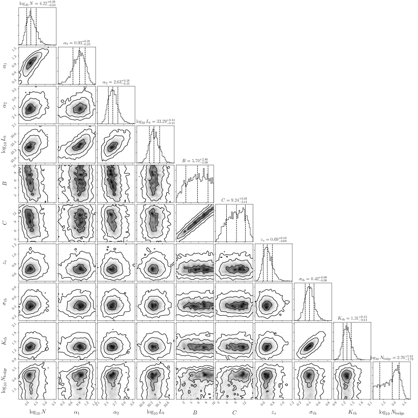
In this section we show corner plots similar to Fig. 2 for a selection of different models considered in the main text. Only changes with respect to the benchmark model are mentioned. In Fig. 9 we show the result for the model with a log-normal luminosity function. Figure 10 contains the results for a model with a Gaussian disk profile. The results for a model including a bulge component is displayed in Fig. 11. Finally, we show the results obtained when using a pulsar sample consisting only of the 2PC MSPs (Fig. 12) and with the addition of unassociated sources (Fig. 13).

Figure 9: Similar to Fig. 2, but for the log-normal luminosity function.

Figure 10: Similar to Fig. 2, but using a Gaussian radial profile for the disk

Figure 11: Similar to Fig. 2, but including an additional bulge component in the center with an identical luminosity function.

Figure 12: Similar to Fig. 2, but using a smaller dataset based on the MSPs in the 2PC (Abdo et al., 2013).

Figure 13: Similar to Fig. 2, but using a larger source sample including unassociated sources selected from Saz Parkinson et al. (2016).

References

- Abazajian (2011) Abazajian, K. N. 2011, The Consistency of Fermi-LAT Observations of the Galactic Center with a Millisecond Pulsar Population in the Central Stellar Cluster, JCAP, 1103, 010
- Abdo et al. (2009a) Abdo, A. A., et al. 2009a, Pulsed Gamma-rays from the millisecond pulsar J0030+0451 with the Fermi Large Area Telescope, Astrophys. J., 699, 1171
- Abdo et al. (2009b) —. 2009b, A Population of Gamma-Ray Millisecond Pulsars Seen with the Fermi Large Area Telescope, Science, 325, 848
- Abdo et al. (2013) —. 2013, The Second Fermi Large Area Telescope Catalog of Gamma-ray Pulsars, Astrophys. J. Suppl., 208, 17
- Acero et al. (2015) Acero, F., et al. 2015, Fermi Large Area Telescope Third Source Catalog, Astrophys. J. Suppl., 218, 23
- Ajello et al. (2017) Ajello, M., et al. 2017, Characterizing the population of pulsars in the inner Galaxy with the Fermi Large Area Telescope, Submitted to: Astrophys. J., arXiv:1705.00009
- Bartels et al. (2018) Bartels, R., Hooper, D., Linden, T., et al. 2018, Comment on ”Characterizing the population of pulsars in the Galactic bulge with the Fermi Large Area Telescope” [arXiv:1705.00009v1], Phys. Dark Univ., 20, 88
- Bartels et al. (2016) Bartels, R., Krishnamurthy, S., & Weniger, C. 2016, Strong support for the millisecond pulsar origin of the Galactic center GeV excess, Phys. Rev. Lett., 116, 051102
- Bartels et al. (2017) Bartels, R., Storm, E., Weniger, C., & Calore, F. 2017, The Fermi-LAT GeV Excess Traces Stellar Mass in the Galactic Bulge, arXiv:1711.04778
- Bhattacharya & van den Heuvel (1991) Bhattacharya, D., & van den Heuvel, E. P. J. 1991, Formation and evolution of binary and millisecond radio pulsars, Phys. Rep., 203, 1
- Buchner et al. (2014) Buchner, J., Georgakakis, A., Nandra, K., et al. 2014, X-ray spectral modelling of the AGN obscuring region in the CDFS: Bayesian model selection and catalogue, Astron. Astrophys., 564, A125
- Calore et al. (2015) Calore, F., Cholis, I., & Weniger, C. 2015, Background Model Systematics for the Fermi GeV Excess, JCAP, 1503, 038
- Calore et al. (2014) Calore, F., Di Mauro, M., & Donato, F. 2014, Diffuse gamma-ray emission from galactic pulsars, Astrophys. J., 796, 1
- Calore et al. (2016) Calore, F., Di Mauro, M., Donato, F., Hessels, J. W. T., & Weniger, C. 2016, Radio detection prospects for a bulge population of millisecond pulsars as suggested by Fermi LAT observations of the inner Galaxy, Astrophys. J., 827, 143
- Caraveo (2014) Caraveo, P. A. 2014, Gamma-ray Pulsar Revolution, Ann. Rev. Astron. Astrophys., 52, 211
- Cholis et al. (2014) Cholis, I., Hooper, D., & Linden, T. 2014, A New Determination of the Spectra and Luminosity Function of Gamma-Ray Millisecond Pulsars, arXiv:1407.5583
- Cholis et al. (2015) —. 2015, Challenges in Explaining the Galactic Center Gamma-Ray Excess with Millisecond Pulsars, JCAP, 1506, 043
- Clark et al. (2018) Clark, C. J., et al. 2018, Einstein@Home discovers a radio-quiet gamma-ray millisecond pulsar, Sc. Adv., 4, eaao7228
- Cognard et al. (2011) Cognard, I., et al. 2011, Discovery of two millisecond pulsars in Fermi sources with the Nancay Radio Telescope, Astrophys. J., 732, 47
- Cordes & Chernoff (1997) Cordes, J. M., & Chernoff, D. F. 1997, Neutron star population dynamics. I: Millisecond pulsars, Astrophys. J., 482, 971
- Cordes & Lazio (2002) Cordes, J. M., & Lazio, T. J. W. 2002, NE2001. 1. A New model for the galactic distribution of free electrons and its fluctuations, arXiv:astro-ph/0207156
- Daylan et al. (2016) Daylan, T., Finkbeiner, D. P., Hooper, D., et al. 2016, The characterization of the gamma-ray signal from the central Milky Way: A case for annihilating dark matter, Phys. Dark Univ., 12, 1
- Eckner et al. (2017) Eckner, C., et al. 2017, Millisecond pulsar origin of the Galactic center excess and extended gamma-ray emission from Andromeda - a closer look, arXiv:1711.05127
- Faucher-Giguere & Loeb (2010) Faucher-Giguere, C. A., & Loeb, A. 2010, The Pulsar Contribution to the Gamma-Ray Background, JCAP, 1001, 005
- Feroz et al. (2009) Feroz, F., Hobson, M. P., & Bridges, M. 2009, MultiNest: an efficient and robust Bayesian inference tool for cosmology and particle physics, Mon. Not. Roy. Astron. Soc., 398, 1601
- Goodenough & Hooper (2009) Goodenough, L., & Hooper, D. 2009, Possible Evidence For Dark Matter Annihilation In The Inner Milky Way From The Fermi Gamma Ray Space Telescope, arXiv:0910.2998
- Gordon & Macias (2013) Gordon, C., & Macias, O. 2013, Dark Matter and Pulsar Model Constraints from Galactic Center Fermi-LAT Gamma Ray Observations, Phys. Rev., D88, 083521, [Erratum: Phys. Rev.D89,no.4,049901(2014)]
- Gorski et al. (2005) Gorski, K. M., Hivon, E., Banday, A. J., et al. 2005, HEALPix - A Framework for high resolution discretization, and fast analysis of data distributed on the sphere, Astrophys. J., 622, 759
- Grégoire & Knödlseder (2013) Grégoire, T., & Knödlseder, J. 2013, Constraining the Galactic millisecond pulsar population using Fermi Large Area Telescope, Astron. Astrophys., 554, A62
- Guillemot et al. (2013) Guillemot, L., Kramer, M., Johnson, T. J., et al. 2013, Fermi LAT pulsed detection of PSR J0737-3039A in the double pulsar system, Astrophys. J., 768, 169
- Hobson et al. (2002) Hobson, M. P., Bridle, S. L., & Lahav, O. 2002, Combining cosmological datasets: hyperparameters and bayesian evidence, Mon. Not. Roy. Astron. Soc., 335, 377
- Hooper et al. (2013) Hooper, D., Cholis, I., Linden, T., Siegal-Gaskins, J., & Slatyer, T. 2013, Pulsars Cannot Account for the Inner Galaxy’s GeV Excess, Phys. Rev., D88, 083009
- Hooper & Linden (2016) Hooper, D., & Linden, T. 2016, The Gamma-Ray Pulsar Population of Globular Clusters: Implications for the GeV Excess, JCAP, 1608, 018
- Hooper & Mohlabeng (2016) Hooper, D., & Mohlabeng, G. 2016, The Gamma-Ray Luminosity Function of Millisecond Pulsars and Implications for the GeV Excess, JCAP, 1603, 049
- Kass & Raftery (1995) Kass, R. E., & Raftery, A. E. 1995, Bayes Factors, Journal of the American Statistical Association, 90, 773. http://www.jstor.org/stable/2291091
- Kuiper et al. (2000) Kuiper, L., Hermsen, W., Verbunt, F., et al. 2000, The Likely detection of pulsed high-energy gamma-ray emission from millisecond pulsar PSR J0218+4232, Astron. Astrophys., 359, 615
- Lee et al. (2016) Lee, S. K., Lisanti, M., Safdi, B. R., Slatyer, T. R., & Xue, W. 2016, Evidence for Unresolved -Ray Point Sources in the Inner Galaxy, Phys. Rev. Lett., 116, 051103
- Levin et al. (2013) Levin, L., et al. 2013, The High Time Resolution Universe Pulsar Survey VIII: The Galactic millisecond pulsar population, Mon. Not. Roy. Astron. Soc., 434, 1387
- Licquia & Newman (2015) Licquia, T. C., & Newman, J. A. 2015, Improved Estimates of the Milky Way’s Stellar Mass and Star Formation Rate From Hierarchical Bayesian Meta-analysis, Astrophys. J., 806, 96
- Lorimer (2001) Lorimer, D. R. 2001, Binary and millisecond pulsars at the new millennium, Living Rev. Rel., 4, 5
- Lorimer (2003) —. 2003, The galactic population and birth rate of radio pulsars, arXiv:astro-ph/0308501, [IAU Symp.218,105(2004)]
- Lorimer et al. (2006) Lorimer, D. R., et al. 2006, The Parkes multibeam pulsar survey: VI. Discovery and timing of 142 pulsars and a Galactic population analysis, Mon. Not. Roy. Astron. Soc., 372, 777
- Lorimer et al. (2015) —. 2015, The Parkes multibeam pulsar survey – VII. Timing of four millisecond pulsars and the underlying spin-period distribution of the Galactic millisecond pulsar population, Mon. Not. Roy. Astron. Soc., 450, 2185
- Lyne et al. (1998) Lyne, A. G., Manchester, R. N., Lorimer, D. R., et al. 1998, The Parkes Southern Pulsar Survey - II. Final results and population analysis, MNRAS, 295, 743
- Macias et al. (2018) Macias, O., Gordon, C., Crocker, R. M., et al. 2018, X-Shaped Bulge Preferred Over Dark Matter for the Galactic Center Gamma-Ray Excess, Nat. Astron., 2, 387
- Manchester et al. (2005) Manchester, R. N., Hobbs, G. B., Teoh, A., & Hobbs, M. 2005, The Australia Telescope National Facility pulsar catalogue, Astron. J., 129, 1993
- McCann (2015) McCann, A. 2015, A stacked analysis of 115 pulsars observed by the Fermi LAT, Astrophys. J., 804, 86
- Nolan et al. (2012) Nolan, P. L., Abdo, A. A., Ackermann, M., et al. 2012, Fermi Large Area Telescope Second Source Catalog, Astrophys. J. Suppl., 199, 31
- Petrović et al. (2015) Petrović, J., Serpico, P. D., & Zaharijas, G. 2015, Millisecond pulsars and the Galactic Center gamma-ray excess: the importance of luminosity function and secondary emission, JCAP, 1502, 023
- Pletsch et al. (2012) Pletsch, H. J., et al. 2012, Binary Millisecond Pulsar Discovery via Gamma-Ray Pulsations, Science, 338, 1314
- Ploeg et al. (2017) Ploeg, H., Gordon, C., Crocker, R., & Macias, O. 2017, Consistency Between the Luminosity Function of Resolved Millisecond Pulsars and the Galactic Center Excess, JCAP, 1708, 015
- Roberts (2011) Roberts, M. S. E. 2011, New Black Widows and Redbacks in the Galactic Field, in American Institute of Physics Conference Series, Vol. 1357, American Institute of Physics Conference Series, ed. M. Burgay, N. D’Amico, P. Esposito, A. Pellizzoni, & A. Possenti, 127–130
- Sanpa-arsa (2016) Sanpa-arsa, S. 2016, PhD thesis, University of Virginia. http://dx.doi.org/10.18130/V36K7P
- Saz Parkinson et al. (2016) Saz Parkinson, P. M., Xu, H., Yu, P. L. H., et al. 2016, Classification and Ranking of Fermi LAT Gamma-ray Sources from the 3FGL Catalog using Machine Learning Techniques, Astrophys. J., 820, 8
- Siegal-Gaskins et al. (2011) Siegal-Gaskins, J. M., Reesman, R., Pavlidou, V., Profumo, S., & Walker, T. P. 2011, Anisotropies in the gamma-ray sky from millisecond pulsars, Mon. Not. Roy. Astron. Soc., 415, 1074
- Story et al. (2007) Story, S. A., Gonthier, P. L., & Harding, A. K. 2007, Population synthesis of radio and gamma-ray millisecond pulsars from the Galactic disk, Astrophys. J., 671, 713
- Taylor & Cordes (1993) Taylor, J. H., & Cordes, J. M. 1993, Pulsar distances and the galactic distribution of free electrons, Astrophys. J., 411, 674
- Trotta (2008) Trotta, R. 2008, Bayes in the sky: Bayesian inference and model selection in cosmology, Contemp. Phys., 49, 71
- Verbiest et al. (2012) Verbiest, J. P. W., Weisberg, J. M., Chael, A. A., Lee, K. J., & Lorimer, D. R. 2012, On Pulsar Distance Measurements and their Uncertainties, Astrophys. J., 755, 39
- Wang et al. (2018) Wang, P., Li, D., Zhu, W., et al. 2018, FAST’s Discovery of a New Millisecond Pulsar (MSP) toward the Fermi-LAT unassociated source 3FGL J0318.1+0252, The Astronomer’s Telegram, 11584
- Winter et al. (2016) Winter, M., Zaharijas, G., Bechtol, K., & Vandenbroucke, J. 2016, Estimating the GeV Emission of Millisecond Pulsars in Dwarf Spheroidal Galaxies, Astrophys. J., 832, L6
- Yao et al. (2017) Yao, J. M., Manchester, R. N., & Wang, N. 2017, A New Electron-density Model for Estimation of Pulsar and FRB Distances, ApJ, 835, 29
- Yuan & Zhang (2014) Yuan, Q., & Zhang, B. 2014, Millisecond pulsar interpretation of the Galactic center gamma-ray excess, JHEAp, 3-4, 1