Scalable Spectral Clustering Using Random Binning Features

Abstract.

Spectral clustering is one of the most effective clustering approaches that capture hidden cluster structures in the data. However, it does not scale well to large-scale problems due to its quadratic complexity in constructing similarity graphs and computing subsequent eigendecomposition. Although a number of methods have been proposed to accelerate spectral clustering, most of them compromise considerable information loss in the original data for reducing computational bottlenecks. In this paper, we present a novel scalable spectral clustering method using Random Binning features (RB) to simultaneously accelerate both similarity graph construction and the eigendecomposition. Specifically, we implicitly approximate the graph similarity (kernel) matrix by the inner product of a large sparse feature matrix generated by RB. Then we introduce a state-of-the-art SVD solver to effectively compute eigenvectors of this large matrix for spectral clustering. Using these two building blocks, we reduce the computational cost from quadratic to linear in the number of data points while achieving similar accuracy. Our theoretical analysis shows that spectral clustering via RB converges faster to the exact spectral clustering than the standard Random Feature approximation. Extensive experiments on 8 benchmarks show that the proposed method either outperforms or matches the state-of-the-art methods in both accuracy and runtime. Moreover, our method exhibits linear scalability in both the number of data samples and the number of RB features.

1. Introduction

Clustering is one of the most fundamental problems in machine learning and data mining tasks. In the past two decades, spectral clustering (SC) (Shi and Malik, 2000; Ng et al., 2002; Von Luxburg, 2007; Chen and Wu, 2017) has shown great promise for learning hidden cluster structures from data. The superior performance of SC roots in exploiting non-linear pairwise similarity between data instances, while traditional methods like K-means heavily rely on Euclidean geometry and thus place limitations on the shape of the clusters (Fowlkes et al., 2004; Yan et al., 2009; Chen and Hero, 2016). However, SC methods are typically not the first choice for large-scale clustering problems since modern datasets exhibit great challenges in both computation and memory consumption for computing the pairwise similarity matrix $\mathbf{W}\in\mathbb{R}^{N\times N}$, where $N$ denotes the number of data points. In particular, given a data matrix $\mathbf{X}\in\mathbb{R}^{N\times d}$ whose underlying data distribution can be represented as $K$ weakly inter-connected clusters, it requires $O(N^{2})$ space to store the matrix and $O(N^{2}d)$ complexity to compute $\mathbf{W}$, and at least takes $O(KN^{2})$ or $O(N^{3})$ complexity to compute $K$ eigenvectors of the corresponding graph Laplacian matrix $\mathbf{L}$, depending on whether an iterative or a direct eigensolver is used. To accelerate SC, many efforts have been devoted to address the following computational bottlenecks: 1) pairwise similarity graph construction of $\mathbf{W}$ from the raw data $\mathbf{X}$, and 2) eigendecomposition of the graph Laplacian matrix $\mathbf{L}$.

A number of methods have been proposed to accelerate the eigendecomposition, e.g., randomized sketching and power method (Gittens et al., 2013; Lin and Cohen, 2010), sequential reduction algorithm toward an early-stop strategy (Chen et al., 2006; Liu et al., 2007), and graph filtering of random signals (Tremblay et al., 2016). However, these approaches only partially reduce the computation cost of the eigendecomposition, since the construction of similarity graph matrix $\mathbf{W}$ still requires quadratic complexity for both computation and memory consumption.

Another family of research is the use of Landmarks or representatives to jointly improve the computation efficiency of the similarity matrix $\mathbf{W}$ and the eigendecomposition of $\mathbf{L}$. One strategy is performing random sampling or K-means on the dataset to select a small number of representative data points and then employing SC on the reduced dataset (Yan et al., 2009; Shinnou and Sasaki, 2008). Another strategy (Sakai and Imiya, 2009; Chen and Cai, 2011; Liu et al., 2013; Li et al., 2016) is approximating the similarity matrix $\mathbf{W}$ by a low rank affinity matrix $\mathbf{Z}\in\mathbb{R}^{N\times R}$, which is computed via either random projection or a bipartite graph between all data points and selected anchor points (Liu et al., 2010). Furthermore, a heuristic that only selects a few nearest anchor points has been applied to build a KNN-based sparse graph similarity matrix. Despite promising results in accelerating SC, these approaches disregard considerable information in the raw data and may lead to degrading clustering performance. More importantly, there is no guarantee that these heuristic methods can approach the results of standard SC.

Another line of research (Fowlkes et al., 2004; Chitta et al., 2012, 2011; Wu et al., 2018a, b) focuses on leveraging various kernel approximation techniques such as Nyström (Williams and Seeger, 2001), Random Fourier (Rahimi and Recht, 2008; Wu et al., 2016; Chen et al., 2016), and random sampling to accelerate similarity matrix construction and the eigendecomposition at the same time. The pairwise similarity (kernel) matrix $\mathbf{W}$ (a weighted fully-connected graph) is then directly approximated by an inner product of the feature matrix $\mathbf{Z}$ computed from the raw data. Although a KNN-based graph construction allows efficient sparse representation, pairwise method takes full advantage of more complete information in the data and takes into account the long-range connections (Fowlkes et al., 2004; Chen et al., 2011). The drawback of pairwise methods is the high computational costs in requiring the similarity between every pair of data points. Fortunately, we present an approximation technique applicable to SC that significantly alleviates this computational bottleneck. As our work focuses on enabling the scalability of SC using RB, the case of robust spectral clustering on noisy data, such as (Bojchevski et al., 2017), could be applied but is beyond the scope of this paper.

In this paper, inspired by recent advances in the fields of kernel approximation and numerical linear algebra (Rahimi and Recht, 2008; Wu et al., 2016; Wu and Stathopoulos, 2015; Wu et al., 2017; Chen et al., 2018), we present a scalable spectral clustering method and theoretic analysis to circumvent the two computational bottlenecks of SC in large-scale datasets. We highlight the following main contributions:

1. We present for the first time the use of Random Binning features (RB) (Rahimi and Recht, 2008; Wu et al., 2016) for scaling up the graph construction of similarity matrix in SC, which is implicitly approximated by the inner product of the RB sparse feature matrix $\mathbf{Z}\in\mathbb{R}^{N\times D}$ derived from the raw dataset, where each row has $nnz(\mathbf{Z}(i,:))=R$. To this end, we reduce the computational complexity of the pairwise graph construction from $O(N^{2}d)$ to $O(NRd)$ and memory consumption from $O(N^{2})$ to $NR$.

2. We further show how to make full use of state-of-the-art near-optimal eigensolver PRIMME (Stathopoulos and McCombs, 2010; Wu et al., 2017) to efficiently compute the eigenvectors of the corresponding graph Laplacian $\mathbf{L}$ without explicit formulation. As a result, the computational complexity of the eigendecomposition is reduced from $O(KN^{2}m)$ to $O(KNRm)$, where $m$ is the number of iterations of the underlying eigensolver.

3. We extend existing analysis of random features to SC from the optimization perspective (Wu et al., 2016), showing a number $R=\Omega(1/(\kappa\epsilon))$ of RB features suffices for the uniform convergence to $\epsilon$ precision of the exact SC.

4. In our extensive experiments on 8 benchmark datasets evaluated by 4 different clustering metrics, the proposed technique either outperforms or matches the state-of-the-art methods in both accuracy and computational time.

5. We corroborate the scalability of our method under two cases: varied number of data samples $N$ and varied number of RB features $R$. In both cases, our method exhibits linear scalability with respect to $N$ or $R$.

2. Spectral Clustering and Random Binning

We briefly introduce the SC algorithms and then illustrate RB, an important building block to our proposed method. Here are some notations we will use throughout the paper.

2.1. Spectral Clustering

Given a set of $N$ data points $[\boldsymbol{x}_{1},\ldots,\boldsymbol{x}_{N}]=\mathbf{X}^{N\times d}$, with $\boldsymbol{x}_{i}\in\mathbb{R}^{d}$, the SC algorithm constructs a similarity matrix $\mathbf{W}\in\mathbb{R}^{N\times N}$ representing an affinity matrix $G=(V,E)$, where the node $\boldsymbol{v}_{i}\in V$ represents the data point $\boldsymbol{x}_{i}$ and the edge $E_{ij}$ represents the similarity between $\boldsymbol{x}_{i}$ and $\boldsymbol{x}_{j}$.

The goal of SC is to use $\mathbf{W}$ to partition $\boldsymbol{x}_{1},\ldots,\boldsymbol{x}_{N}$ into $K$ clusters. There are several variants of SC. Without lose of generality, we consider the widely used normalized spectral clustering (Ng et al., 2002). To fully utilize complete similarity information, we consider a fully connected graph instead of a KNN-based graph for SC. An example similarity (kernel) function is the Gaussian Kernel:

(1) $$k(\boldsymbol{x}_{i},\boldsymbol{x}_{j})=\text{exp}\Big{(}-\frac{\|\boldsymbol{x}_{i}-\boldsymbol{x}_{j}\|^{2}}{2\sigma^{2}}\Big{)}$$

where $\sigma$ is the bandwidth parameter. The normalized graph Laplacian matrix $\mathbf{L}$ is defined as:

(2) $$\mathbf{L}=\mathbf{D}^{-1/2}(\mathbf{D}-\mathbf{W})\mathbf{D}^{-1/2}=\mathbf{I}-\mathbf{D}^{-1/2}\mathbf{W}\mathbf{D}^{-1/2}$$

where $\mathbf{D}\in\mathbb{R}^{N\times N}$ is the degree matrix with each diagonal element $\mathbf{D}_{ii}=\sum_{j=1}^{N}\mathbf{W}_{ij}$. The objective function of normalized SC can be defined as (Shi and Malik, 2000):

(3) $$\min_{\mathbf{U}\in\mathbb{R}^{N\times K},\mathbf{U}^{T}\mathbf{U}=\mathbf{I}}~{}\textnormal{trace}(\mathbf{U}^{T}\mathbf{L}\mathbf{U}),$$

where $\textnormal{trace}(\cdot)$ denotes the matrix trace, $\mathbf{I}$ denotes the identity matrix, and the constraint $\mathbf{U}^{T}\mathbf{U}=\mathbf{I}$ implies orthonormality on the columns of $\mathbf{U}$. We further denote $\mathbf{U}^{*}\in\mathbb{R}^{N\times K}$ as the optimizer of the minimization problem in (3), where the columns of $\mathbf{U}^{*}$ are the $K$ smallest eigenvectors of $\mathbf{L}$. Finally, the K-means method is applied on the rows of $\mathbf{U}^{*}$ to obtain the clusters. The high computational costs of the similarity matrix $O(N^{2}d)$ and the eigendecomposition $O(KN^{2})$ make SC hardly scalable to large-scale problems.

2.2. Random Binning Features

RB features are first introduced in (Rahimi and Recht, 2008) and rediscovered in (Wu et al., 2016) to yield a faster convergence compared to other Random Features methods for scaling up large-scale kernel machine. It considers a feature map of the form

(4) $$k(\boldsymbol{x}_{1},\boldsymbol{x}_{2})=\int_{\boldsymbol{\omega}}p(\boldsymbol{\omega})\boldsymbol{\phi}_{B_{\boldsymbol{\omega}}}(\boldsymbol{x}_{1})^{T}\boldsymbol{\phi}_{B_{\boldsymbol{\omega}}}(\boldsymbol{x}_{2})\;d\boldsymbol{\omega}$$

where a set of bins $B_{\boldsymbol{\omega}}$ defines a random grid that are determined by $\boldsymbol{\omega}=(\omega_{1},u_{1},...,\omega_{d},u_{d})$ drawn from a distribution $p(\boldsymbol{\omega})$, and $(\omega_{i},u_{i})$ represents width and bias in the $i$-th dimension of a grid. Then for any bin $\boldsymbol{b}\in B_{\boldsymbol{\omega}}$, the feature vector $\boldsymbol{\phi}_{B_{\boldsymbol{\omega}}}(\boldsymbol{x})$ has

$$\boldsymbol{\phi}_{\boldsymbol{b}}(\boldsymbol{x}_{i})=1,\;\textit{if}\;\boldsymbol{b}=(\lfloor\frac{\boldsymbol{x}_{i}^{(1)}-u_{1}}{\omega_{1}}\rfloor,...,\lfloor\frac{\boldsymbol{x}_{i}^{(d)}-u_{d}}{\omega_{d}}\rfloor)$$

if the data point $\boldsymbol{x}_{i}$ locates in the bin $\boldsymbol{b}\in B_{\boldsymbol{\omega}}$. Since a data point can only locate in one bin, $\boldsymbol{\phi}_{\boldsymbol{b}}(\boldsymbol{x}_{i})=0$ for any other bins. Note for each grid $B_{\boldsymbol{\omega}}$ the number of bins $|B_{\boldsymbol{\omega}}|$ is countably infinite, therefore $\boldsymbol{\phi}_{B_{\boldsymbol{\omega}}}(\boldsymbol{x})$ has infinite dimensions but only $1$ non-zero entry (at the bin $\boldsymbol{x}$ lies in). Figure 1 illustrates an RB example when the data dimension $d=2$. When two data points $\boldsymbol{x}_{1}$, $\boldsymbol{x}_{2}$ fall in the same bin, the collision probability for this to happen is proportional to the kernel value $k(\boldsymbol{x}_{1},\boldsymbol{x}_{2})$. Note that for a given grid multiple non-empty bins (features) can be produced and thus RB essentially generates a large sparse binary matrix (for more details, please refer to (Wu et al., 2016)).

In practice, in order to obtain a good kernel approximation matrix $\mathbf{Z}$, a simple Monte Carlo method is often leveraged to approximate (4) by averaging over $R$ grids $\{B_{\boldsymbol{\omega}_{i}}\}_{i=1}^{R}$, where each grid’s parameter $\boldsymbol{\omega}_{i}$ is drawn from $p(\boldsymbol{\omega})$. Algorithm 1 summarizes the procedure for generating a number $R$ of RB features from the original dataset $\mathbf{X}$. The resulting feature matrix $\mathbf{Z}\in\mathbb{R}^{N\times D}$, where $D$ is determined jointly by both the number of grids $R$ and the kernel parameter $\sigma$. However, for each row the number of nonzero entries $nnz(\mathbf{Z}(i,:))=R$ and thus the total number of $nnz(\mathbf{Z})=NR$, which is the same as other random feature methods (Wu et al., 2016).

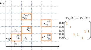
Figure 1. Example of generating RB features when $d=2$.

Algorithm 1 RB Features Generation

1:Input: Given a kernel function $k(\boldsymbol{x}_{i},\boldsymbol{x}_{j})=\prod_{l=1}^{d}k_{l}(|x_{i}^{(l)}-x_{j}^{(l)}|)$. Let $p_{j}(\boldsymbol{\omega})\propto\boldsymbol{\omega}k_{j}^{\prime\prime}(\boldsymbol{\omega})$ be a distribution over $\boldsymbol{\omega}$.

2:Output: RB feature matrix $\mathbf{Z}^{N\times D}$ for raw data $\mathbf{X}$

3:for $j=1,\ldots,R$ do

4:   Draw $\omega_{i}$ from $p_{j}(\boldsymbol{\omega})$ and $u_{i}\in[0,\omega_{i}]$, for $\forall i\in[d]$

5:   Compute feature values $\boldsymbol{z}_{j}(\boldsymbol{x}_{i})$ as the indicator vector of bin index $(\lfloor\frac{\boldsymbol{x}_{i}^{(1)}-u_{1}}{\omega_{1}}\rfloor,...,\lfloor\frac{\boldsymbol{x}_{i}^{(d)}-u_{d}}{\omega_{d}}\rfloor)$, for $\forall i\in[N]$.

6:end for

7:$\mathbf{Z}_{i,:}=\frac{1}{\sqrt{R}}[\boldsymbol{z}_{1}(\boldsymbol{x}_{i});...;\boldsymbol{z}_{D}(\boldsymbol{x}_{i})]$, for $\forall i\in[N]$

3. Scalable Spectral Clustering Using RB Features

In this section, we introduce our proposed scalable SC method, called SC_RB, based on RB and a state-of-the-art sparse eigensolver (PRIMME) to effectively tackle the two computational bottlenecks: 1) Pairwise graph construction; and 2) Eigendecomposition of the graph Laplacian matrix.

3.1. Pairwise graph construction

The first step of SC is to build a similarity graph. A fully connected graph entailing complete similarity information of the original data offers great flexibility in the underlying kernel function to define the affinities between data points. However, constructing a pairwise graph essentially computes a similarity (kernel) matrix between each pair of samples, which is computationally intensive due to its quadratic complexity $O(N^{2}d)$. Thus, we propose to use RB features $\mathbf{Z}$ to approximate the pairwise kernel matrix $\mathbf{W}$, resulting in the following approximate spectral clustering objective:

(5) $$\min_{\mathbf{U}\in\mathbb{R}^{N\times K},\mathbf{U}^{T}\mathbf{U}=\mathbf{I}}~{}\textnormal{trace}(\mathbf{U}^{T}\widehat{\mathbf{L}}\mathbf{U})$$

where

$$\widehat{\mathbf{L}}:=\mathbf{I}-\widehat{\mathbf{D}}^{-1/2}\widehat{\mathbf{W}}\widehat{\mathbf{D}}^{-1/2}=\mathbf{I}-\widehat{\mathbf{D}}^{-1/2}\mathbf{Z}\mathbf{Z}^{T}\widehat{\mathbf{D}}^{-1/2}$$

and $\mathbf{Z}$ is a large sparse $N\times D$ matrix generated from Algorithm 1. To apply RB to SC, it is necessary to compute the degree matrix $\widehat{\mathbf{D}}$, the row sum of $\widehat{\mathbf{W}}$. Luckily, we can compute it without explicitly computing $\mathbf{Z}\mathbf{Z}^{T}$ since

(6) $$\widehat{\mathbf{D}}=\textnormal{diag}(\widehat{\mathbf{W}}\boldsymbol{1})=\textnormal{diag}(\mathbf{Z}(\mathbf{Z}^{T}\boldsymbol{1}))$$

where $\textnormal{diag}(\boldsymbol{x})$ is a diagonal matrix with the vector $\boldsymbol{x}$ on its main diagonal, and $\boldsymbol{1}$ represents a column vector of ones. Therefore, we can simply compute $\widehat{\mathbf{D}}$ by two matrix-vector multiplication without the explicit form of $\widehat{\mathbf{W}}$. With $\widehat{\mathbf{D}}$, we define $\widehat{\mathbf{Z}}=\widehat{\mathbf{D}}^{-1/2}\mathbf{Z}$ and thus we approximate the graph Laplacian matrix with $\widehat{\mathbf{L}}=\mathbf{I}-\widehat{\mathbf{Z}}\widehat{\mathbf{Z}}^{T}$ in linear complexity.

3.2. Effective eigendecomposition using PRIMME

After constructing the pairwise graph implicitly using $\mathbf{Z}$, we compute the largest left singular vectors of $\widehat{\mathbf{Z}}$, which is equivalent to computing the smallest eigenvectors of $\widehat{\mathbf{L}}:=\mathbf{I}-\widehat{\mathbf{Z}}\widehat{\mathbf{Z}}^{T}$ in Equation (5), satisfying

(7) $$\widehat{\mathbf{Z}}\boldsymbol{v}_{i}=\sigma_{i}\boldsymbol{u}_{i},\quad\quad i=1,\ldots,K,\ \ K\ll N,$$

where the singular values are labeled in descending order, $\sigma_{1}\geq\sigma_{2}\geq\ldots\geq\sigma_{K}$. The matrices $\mathbf{U}=[\boldsymbol{u}_{1},\ldots,\boldsymbol{u}_{K}]\in\mathbb{R}^{N\times K}$ and $\mathbf{V}=[\boldsymbol{v}_{1},\ldots,\boldsymbol{v}_{n}]\in\mathbb{R}^{D\times K}$ are the left and right singular vectors respectively, where $\mathbf{U}$ is the low-dimensional embedding associated with $K$ clusters.

However, $\widehat{\mathbf{Z}}$, a weighted RB feature matrix of $\mathbf{Z}$, is a very large sparse matrix of the size $N\times D$, making it a challenging task for any standard SVD solver. Specifically, one has to resort to a powerful iterative sparser eigensolver that is capable to handle two difficulties for large-scale matrix: 1) slow convergence of eigenvalues when the eigenvalue gaps are not well separated, a common case when $N$ is large; 2) low memory footprint yet near-optimal convergence for seeking a small number of eigenpairs.

To overcome these challenges, we leverage current state-of-the-art eigenvalue and SVD solver (Stathopoulos and McCombs, 2010; Wu et al., 2017), named PReconditioned Iterative MultiMethod Eigensolver (PRIMME). It implements two near-optimal eigenmethods GD+K and JDQMR that are default methods for seeking a small portion of extreme eigenpairs under limited memory. Unlike Lanczos methods (like Matlab svds function), these eigenmethods are in the classes of Generalized Davidson, which enjoy benefits for advanced subspace restarting and preconditioning techniques to accelerate the convergence.

Once the left singular vectors $\mathbf{U}$ are obtained, following (Ng et al., 2002), we obtain $\widehat{\mathbf{U}}$ by normalizing each row of $\mathbf{U}$ to unit norm. Then K-means method is applied to the rows of $\widehat{\mathbf{U}}$ to obtain the final $K$ clusters and the binary membership matrix $\mathbf{M}\in\{0,1\}^{N\times K}$.

Algorithm 2 Scalable SC method based on RB

1:Input: Data matrix $\mathbf{X}$, number of clusters $K$, number of girds $R$, kernel parameter $\sigma$.

2:Output: K clusters and membership matrix $\mathbf{M}$

3:Construct a fully connected graph using a sparse feature matrix $\mathbf{Z}\in\mathbb{R}^{N\times D}$ generated by RB using Algorithm 1.

4:Compute degree matrix $\widehat{\mathbf{D}}$ using Equation 6 and obtain $\widehat{\mathbf{Z}}=\widehat{\mathbf{D}}^{-1/2}\mathbf{Z}$ using Equation 5.

5:Compute $K$ largest left singular vectors $\mathbf{U}$ of $\widehat{\mathbf{Z}}$ using state-of-the-art iterative sparse SVD solver (e.g., PRIMME).

6:Obtain the matrix $\widehat{\mathbf{U}}$ from $\mathbf{U}$ by row normalization.

7:Cluster the rows of $\widehat{\mathbf{U}}$ into $K$ clusters using K-means and obtain the corresponding membership matrix $\mathbf{M}$.

Computation analysis. Algorithm 2 summarizes the procedure for the proposed scalable SC method based on RB and PRIMME. Using these two important building blocks, the computational complexity has been substantially reduced from $O(N^{2}d)$ to $O(NRd+NR)$ for computing the feature matrix $\widehat{\mathbf{Z}}$ from RB in pairwise graph construction, and from at least $O(KN^{2}m)$ to $O(KNRm)$ for the subsequent SVD computation, where $m$ is the number of iterations of the underlying SVD solver. At the same time, the memory consumption has been reduced from $O(N^{2})$ to $O(NR)$. In addition to these two key steps, the final K-means also takes $O(NK^{2}t)$, where $t$ is the number of iterations of K-means. Therefore, the total computational complexity and memory consumption are $O(NRd+NKRm+NK^{2}t)$ and $O(NR)$. The linear complexity in the number $N$ of data points render SC scalable to large-scale problems.

4. Theoretical Analysis

The convergence of Random Feature approximation has been studied since it was first proposed in (Rahimi and Recht, 2008), where a sampling approximation analysis was employed to show the convergence of the approximation to exact kernel. Such analysis was adopted by most of its follow-up works. More recently, a new approach of analysis based on infinite-dimensional optimization is proposed in (Yen et al., 2014), which achieves a faster convergence rate than the previous approach, and was employed further in (Wu et al., 2016) to explain the superior convergence of Random Binning Features than other types of random features in the context of classification.

Here we further adapt the analysis in (Wu et al., 2016) to study the convergence of Spectral Clustering under RB approximation. We first recall the well-known connection between SC and kernel $K$-means (Dhillon et al., 2004), stating the equivalence of (3) to the following objective

(8) $$\min_{\mathbf{U}\in\mathbb{R}^{N\times K}:\mathbf{U}^{T}\mathbf{U}=\mathbf{I}}\min_{\mathcal{M}} \frac{1}{2N}\sum_{i=1}^{N}\|\boldsymbol{\phi}(\boldsymbol{x}_{i})-\mathcal{M}\mathbf{U}_{i,:}^{T}\|^{2}$$

where $\boldsymbol{\phi}(.)$ is a possibly infinite-dimensional feature map in (4) from the normalized kernel, $\mathcal{M}$ is the matrix of means with $k$ columns, each of which has the same dimension to the feature map $\boldsymbol{\phi}(.)$. Dropping constants that are neither related to $\mathbf{U}$ nor related to $\mathcal{M}$, the objective (8) becomes

(9) $$f(\mathbf{U},\mathcal{M}):=\frac{1}{N}\sum_{i=1}^{N}-\langle\boldsymbol{\phi}(\boldsymbol{x}_{i}),\mathcal{M}\mathbf{U}_{i,:}^{T}\rangle+\frac{1}{2N}\|\mathcal{M}\mathbf{U}_{i,:}\|^{2}.$$

Let $(\widehat{\mathbf{U}},\widehat{\mathcal{M}})$ be the clustering from the RB approximation:

(10) $$(\widehat{\mathbf{U}},\widehat{\mathcal{M}}):=\underset{\mathbf{U},\mathcal{M}}{\arg\min}\;\frac{1}{N}\sum_{i=1}^{N}-\langle\boldsymbol{z}(\boldsymbol{x}_{i}),\mathcal{M}\mathbf{U}_{i,:}^{T}\rangle+\frac{1}{2N}\|\mathcal{M}\mathbf{U}_{i,:}\|^{2}$$

Let $(\mathbf{U}^{*},\mathcal{M}^{*})$ be the exact minimizer of (9). Our goal is to show that

(11) $$f(\widehat{\mathbf{U}},\widehat{\mathcal{M}})\leq f(\mathbf{U}^{*},\mathcal{M}^{*})+\epsilon$$

as long as the number of Random Binning grids satisfies $R=\Omega(\frac{1}{\kappa\epsilon})$, where $\kappa$ is an estimate of the number of non-empty bins per grid. The quantity $\kappa$ is crucial in the our analysis, as under the same computational budget, RB generates $\kappa$ more features in expectation and converges $\kappa$-times faster than other types of random features. Note the computational cost is not $\kappa$-times more because of the sparse structure of RB—only one of $\kappa$ features is non-zero for each sample $\boldsymbol{x}$. The formal definition of $\kappa$ is as follows.

Definition 0.

Define the collision probability of data $\mathbf{X}$ on bin $b\in B_{\boldsymbol{\delta}}$ as:

(12) $$\nu_{b}:=\frac{|\{n\in[N]\;|\;\phi_{b}=1\}|}{N}.$$

Let $\nu_{\boldsymbol{\delta}}:=\max_{b\in B_{\boldsymbol{\delta}}}\nu_{b}$ be an upper bound on (12), and $\kappa_{\boldsymbol{\delta}}:=1/\nu_{\boldsymbol{\delta}}$ be a lower bound on the number of non-empty bins of grid $B_{\boldsymbol{\delta}}$. Then

(13) $$\kappa:=E_{\boldsymbol{\delta}}[\kappa_{\boldsymbol{\delta}}]\geq 1$$

is the expected number of non-empty bins.

The proof of (11) contains two parts. In the first part, we show that $f(\mathbf{U},\widehat{\mathcal{M}})\leq f(\mathbf{U},\mathcal{M}^{*})+\epsilon$ for any given $\mathbf{U}$. This is obtained from the insight that the RB approximation $\boldsymbol{z}(\boldsymbol{x})$ (from Algorithm 1) is a subset of coordinates from the feature map $\boldsymbol{\phi}(\boldsymbol{x})$. Therefore, $\widehat{\mathcal{M}}$ can be interpreted as a solution obtained from $R$ iterations of Randomized Block Coordinate Descent on $f(\mathbf{U},\mathcal{M})$ w.r.t. $\mathcal{M}$, which results in $R$ non-zero blocks of rows in $\mathcal{M}$.

Theorem 2.

Let $R$ be the number of grids generated by Algorithm 1. For any given $\mathbf{U}$, let $\mathcal{M}^{*}$ and $\widehat{\mathcal{M}}$ be the minimizers of (8) and (10) respectively. We have

(14) $$E[f(\mathbf{U},\widehat{\mathcal{M}})]-f(\mathbf{U},\mathcal{M}^{*})\leq\frac{\|\mathcal{M}^{*}\|_{F}^{2}}{\kappa(R-c)}$$

for $R>c$, where $c$ is a small constant.

Proof.

Let $\mathbf{\Phi}:=[\boldsymbol{\phi}(\boldsymbol{x}_{1}),...,\boldsymbol{\phi}(\boldsymbol{x}_{N})]$. Given $\mathbf{U}$ that satisfies $\mathbf{U}^{T}\mathbf{U}=\mathbf{I}$, the objective $f(\mathbf{U},\mathcal{M})$ can be written as

$$f(\mathbf{U},\mathcal{M}) =\frac{-1}{N}\langle\mathbf{\Phi},\mathcal{M}\mathbf{U}^{T}\rangle+\frac{1}{2N}\textnormal{trace}(\mathcal{M}\mathbf{U}^{T}\mathbf{U}\mathcal{M}^{T})$$

$$=\frac{-1}{N}\langle\mathbf{\Phi}\mathbf{U},\mathcal{M}\rangle+\frac{1}{2N}\|\mathcal{M}\|_{F}^{2}$$

$$=\sum_{k=1}^{K}g(\mathbf{U}_{:,k},\mathcal{M}_{:,k}),$$

where $g(\mathbf{U}_{:,k},\mathcal{M}_{:,k})$ is defined as

(15) $$\frac{1}{N}\sum_{i=1}^{N}-\langle\boldsymbol{\phi}(\boldsymbol{x}_{i})u_{ik},\mathcal{M}_{:,k}\rangle+\frac{1}{2N}\|M_{:,k}\|^{2}.$$

In other words, given $\mathbf{U}$, $f(\mathbf{U},\mathcal{M})$ can be separated as $K$ independent subproblems, each solving a column of $\mathcal{M}$. Let the first term of (15) be the loss function and the second term be the regularizer. Then (15) satisfies the form of a convex, smooth empirical loss minimization problem studied in (Wu et al., 2016). By Theorem 1 of (Wu et al., 2016), the minimizer of (15) satisfies

(16) $$E[g(\mathbf{U}_{:,k},\widehat{\mathcal{M}}_{:,k})]-g(\mathbf{U}_{:,k},\mathcal{M}_{:,k}^{*})\leq\frac{\|\mathcal{M}^{*}_{:,k}\|^{2}}{\kappa(R-c_{k})}$$

with $c_{k}:=\lceil\frac{2\kappa(g(\mathbf{U}_{:,k},\boldsymbol{0})-g(\mathbf{U}_{:,k},\mathcal{M}^{*}_{:,k}))}{\|\mathcal{M}_{:,k}^{*}\|^{2}}\rceil$. Summing (16) over $k=1...K$, we have

$$E[f(\mathbf{U},\widehat{\mathcal{M}})]-f(\mathbf{U},\mathcal{M}^{*})\leq\frac{\|\mathcal{M}^{*}\|_{F}^{2}}{\kappa(R-c)}$$

where $c:=\max_{k=1}^{K}c_{k}$. ∎

Theorem 2 implies that $f(\mathbf{U},\widehat{\mathcal{M}})\leq f(\mathbf{U},\mathcal{M}^{*})+\epsilon$ for

(17) $$R_{RB}\geq\frac{\|\mathcal{M}^{*}\|_{F}^{2}}{\kappa\epsilon}+c.$$

As noted by the earlier work (Wu et al., 2016), this convergence rate is $\kappa$ times faster than that of other Random Features under the same analysis framework. More specifically, if applying Theorem 2 of (Yen et al., 2014) instead of Theorem 1 of (Wu et al., 2016) in the proof of Theorem 2, one would have obtained a $\kappa$-times slower convergence rate for a general Random Feature method that generates a single feature at a time, which requires

$$R_{RF}\geq\frac{\|\mathcal{M}^{*}\|_{F}^{2}}{\epsilon}+c^{\prime}$$

number of features to guarantee an $\epsilon$ suboptimality. This is owing to RB’s ability to generate a block of $\kappa$ expected number of features at a time.

In the second part of the proof, we show that the spectral clustering $\widehat{\mathbf{U}}$ obtained from the RB approximation converges to $\mathbf{U}^{*}$ in the objective.

Theorem 3.

Let $R$ be the number of grids generated by Algorithm 1, and let $\mathbf{U}^{*}$, $\widehat{\mathbf{U}}$ be the spectral clusterings obtained from (8), (10) respectively. We have

(18) $$E[f(\widehat{\mathbf{U}},\widehat{\mathcal{M}})]-f(\mathbf{U}^{*},\mathcal{M}^{*})\leq\epsilon$$

for

$$R\geq\frac{\|\mathcal{M}^{*}\|_{F}^{2}}{\kappa\epsilon}+c$$

where $c$ is a small constant (defined in Theorem 2).

Proof.

Note the problem (10) can be solved with global optimal guarantee by finding minimum eigenvalues and eigenvectors of (5). Therefore, let $\widehat{\mathcal{M}}(\widehat{\mathbf{U}})$, $\widehat{\mathcal{M}}(\mathbf{U}^{*})$ be the minimizers of (10) under $\widehat{\mathbf{U}}$, $\mathbf{U}^{*}$ respectively. We have

(19) $$f(\widehat{\mathbf{U}},\widehat{\mathcal{M}}(\widehat{\mathbf{U}}))\leq f(\mathbf{U}^{*},\widehat{\mathcal{M}}(\mathbf{U}^{*}))$$

by the optimality of $(\widehat{\mathbf{U}},\widehat{\mathcal{M}}(\widehat{\mathbf{U}}))$ under the approximate feature map $\boldsymbol{z}(\boldsymbol{x})$. In addition, from Theorem 2 we have

(20) $$f(\mathbf{U}^{*},\widehat{\mathcal{M}}(\mathbf{U}^{*}))-f(\mathbf{U}^{*},\mathcal{M}^{*})\leq\frac{\|\mathcal{M}^{*}\|_{F}^{2}}{\kappa(R-c)}$$

for $R>c$. Combining (19) and (20) leads to the result. ∎

5. Experiments

We conduct experiments to demonstrate the effectiveness and efficiency of the proposed method, and compare against 8 baselines on 8 benchmarks. Our code is implemented in Matlab and we use C Mex functions for computationally expensive components of RB and of PRIMME eigensolver . All computations are carried out on a linux machine with Intel Xeon CPU at 3.3GHz for a total of 16 cores and 500 GB main memory.

Table 1. Properties of the datasets.

Name	$K$: Classes	$d$: Features	$N$: Samples
pendigits	10	16	10,992
letter	26	16	15,500
mnist	10	780	70,000
acoustic	3	50	98,528
ijcnn1	2	22	126,701
cod_rna	2	8	321,054
covtype-mult	7	54	581,012
poker	10	10	1,025,010

Datasets. As shown in Table 1, we choose 8 datasets from LibSVM (Chang and Lin, 2011), where 5 of them overlap with the datasets used in (Yan et al., 2009; Li et al., 2016; Chen and Cai, 2011). We summarize them as follows:

1) pendigits. A collection of handwritten digit data set consisting of 250 samples from 44 writers where sampled coordination information are used to generate 16 features per sample;

2) letter. A collection of images for 26 capital letters in the English alphabet where 16 character image features are generated;

3) minst. A popular collection of handwritten digit data set distributed by Yann LeCun, where each image is represented by a 784 dimensional vector;

4) acoustic. A collection of time-series data from various sensors in the moving vehicles for measuring the acoustic modality where a 50 dimensional feature vector is generated by using FFT for each time-series;

5) ijcnn1. A collection of time-series data from IJCNN 2001 Challenge, where 22 attributes are generated as a feature vector;

6) cod_rna. A collection of non-coding RNA sequences, where the total 8 features are generated by counting the frequencies of ’A’, ’U’, ’C’ of sequences 1 and 2 as well as the length of the shorter sequence and deltaG_total value;

7) covtype-mult. A collection of samples for predicting the forest cover type from cartographic variables, where the total 54 feature vector is generated for representing a sample;

8) poker. A collection of poker record samples where each hand consisting of five playing cards drawn from a standard deck of 52 generates a feature vector of 10 attributes.

Table 2. Average rank scores comparing SC_RB against others methods using $R=1024$.

Dataset	K-means	SC	KK_RS	KK_RF	SV_RF	SC_LSC	SC_Nys	SC_RF	SC_RB
pendigits	3.00	4.75	2.00	7.75	8.5	1.00	4.75	7.25	5.00
letter	8.50	5.75	5.50	7.50	4.75	3.25	4.75	3.75	1.25
mnist	5.00	4.25	5.00	9.00	8.00	1.00	3.25	6.75	2.75
acoustic	4.75	–	4.25	6.25	5.75	3.50	4.75	5.75	1.00
ijcnn1	4.50	–	5.75	2.00	4.00	6.75	4.75	7.25	1.00
cod_rna	5.75	–	3.50	5.00	7.75	5.50	4.00	2.75	1.75
covtype-mult	3.75	–	5.25	5.75	6.50	2.50	4.75	5.75	1.75
poker	4.33	–	4.00	3.33	4.67	5.67	5.00	4.33	4.67

Table 3. Computational time (seconds) comparing SC_RB against others methods using $R=1024$.

Dataset	K-means	SC	KK_RS	KK_RF	SV_RF	SC_LSC	SC_Nys	SC_RF	SC_RB
pendigits	0.8	25.0	10.7	10.4	1.0	7.6	2.5	1.4	1.8
letter	5.9	171.4	17.1	36.9	8.9	27.1	14.6	10.0	7.7
mnist	278.1	2661	79.1	312.4	22.6	25.5	31.0	20.5	25.9
acoustic	10.2	–	34.7	83.7	6.3	16.7	20.1	7.0	10.7
ijcnn1	4.2	–	44.2	89.6	5.1	9.9	18.5	5.5	34.7
cod_rna	6.7	–	88.2	190.0	8.6	8.9	46.8	13.0	24.2
covtype-mult	60.7	–	180.2	220.0	40.5	181.1	99.1	41.5	1593
poker	102.4	–	363.1	5812	254.5	337.4	340.6	293.3	538.4

Baselines. We compare against 8 random feature based SC or approximation SC methods:

1) SC_Nys (Fowlkes et al., 2004): a fast SC method based on Nyström method;

2) SC_LSC (Chen and Cai, 2011): approximate SC for KNN-based bipartite graph between raw data and anchor points selected by K-means;

3) SV_RF (Chitta et al., 2012): fast kernel K-means using singular vectors of the RF feature matrix (approximating similarity matrix $\mathbf{W}$);

4) SC_RF: we modify SV_RF method to become a fast SC method based on RF feature matrix (approximating Laplacian matrix $\mathbf{L}$);

5) KK_RF (Chitta et al., 2012): another kernel K-means approximation method directly using the RF feature matrix;

6) KK_RS (Chitta et al., 2011): an approximate Kernel K-means by a random sampling approach;

7) SC (Ng et al., 2002): Exact SC method;

8) K-means (Hartigan and Wong, 1979): standard K-means method applied on original dataset.

Evaluation metrics. We use 4 commonly used clustering metrics for cluster quality evaluation, which has been advocated and discussed in (Zaki et al., 2014). Let $\{\mathcal{C}_{k}\}_{k=1}^{K}$ and $\{\mathcal{C}^{\prime}_{k}\}_{k=1}^{K}$ denote the $K$ clusters found by a clustering algorithm and the true cluster labels, respectively. The considered clustering metrics are:

1) Normalized mutual information (NMI):

$$\textnormal{NMI}=\frac{2\cdot I(\{\mathcal{C}_{k}\},\{\mathcal{C}^{\prime}_{k}\})}{|H(\{\mathcal{C}_{k}\})+H(\{\mathcal{C}^{\prime}_{k}\})|},$$

where $I$ is the mutual information between $\{\mathcal{C}_{k}\}_{k=1}^{K}$ and $\{\mathcal{C}^{\prime}_{k}\}_{k=1}^{K}$, and $H$ is the entropy of clusters.

2) Rand index (RI):

$$\textnormal{RI}=\frac{TP+TN}{TP+TN+FP+FN},$$

where $TP$, $TN$, $FP$ and $FN$ represent true positive, true negative, false positive, and false negative decisions, respectively.

3) F-measure (FM):

$$\textnormal{FM}=\frac{1}{K}\sum_{k=1}^{K}\textnormal{F-measure}_{k},$$

where $\textnormal{F-measure}_{k}=\frac{2\cdot PREC_{k}\cdot RECALL_{k}}{PREC_{k}+RECALL_{k}}$, and $PREC_{k}$ and $RECALL_{k}$ are the precision and recall values for cluster $\mathcal{C}_{k}$.

4) Accuracy (Acc):

$$\textnormal{Acc}=\frac{1}{N}\sum_{i=1}^{N}\delta(\{\mathcal{C}_{k}\}_{k=1}^{K},\{\mathcal{C}^{\prime}_{k}\}_{k=1}^{K})$$

where $N$ is the total number of samples and the best mapping function $\delta(x,y)$ is the delta function that equals 1 if $x=y$ and equals 0 otherwise between cluster labels $\{\mathcal{C}_{k}\}_{k=1}^{K}$ and the true labels $\{\mathcal{C}^{\prime}_{k}\}_{k=1}^{K}$ for each sample.

These metrics are all scaled between 0 and 1, and higher value means better clustering.

Average rank score. To combine multiple clustering metrics for performance evaluation of different SC methods, we adopt the methodology proposed in (Yang and Leskovec, 2015) and use the average rank score of all clustering metrics as the final performance metric. Therefore, lower average rank score means better clustering performance.

Parameter selection. We use the RBF kernel for all similarity (Kernel) based methods on all datasets, where the kernel parameter $\sigma$ is obtained through cross-validation within typical range [0.01 100]. All methods use the same kernel parameters to promote a fair comparison. For other parameters, we use the recommended settings in the literature.

5.1. Clustering accuracy and computational time on all datasets

Setup. We first compare against 8 aforementioned baselines in terms of both average rank score and computational time. We use the methodology proposed in (Yang and Leskovec, 2015) to compute the average ranking score among 4 different metrics NMI, RI, FM, and Acc. Although the rank $R$ has different meanings in each method but similar effects on the performance, we choose $R=1024$ for all methods to promote a fair comparison. In addition, we use PRIMME_SVDS to accelerate SVD decomposition for all methods except SC_LSC. For the final step of SC, we use Matlab’s internal K-means function with 10 replicates. All methods use same random seeds so the difference caused by randomness is minimized.

Results. Table 2 shows that SC_RB consistently outperforms or matches state-of-the-art SC methods in terms of average ranking score on 5 out of 8 datasets (except pendigits, mnist, poker). The first highlight in the table is that SC_LSC has quite good performance in the majority of datasets, especially for pendigits and mnist, owing to the sparse low rank approximation using AnchorGraph technique (Liu et al., 2010). However, we would like to point out that in SC_LSC the similarity matrix is built on a KNN-based graph, which is essentially different from other SC methods which use a fully connected graph. This explains why SC_LSC has even better performance than the exact SC method in these two datasets. For poker, all methods have very close numbers in four different metrics, which leads to quite similar average ranking score for all methods. Secondly, the SC type methods such as SC_Nys, SC_RF, and SC_RB generally achieve better ranking scores compared to similarity-based on methods such as KK_RF and SV_RF. This is because the SC type methods are built on a Normalized Cuts formulation that yields a better performance guarantee in terms of the graph clustering. Finally, the improved performance of SC_RB in the majority of datasets stems from the fact that it directly approximate a pairwise similarity matrix, which utilizes all information from the raw data. Its faster convergence allows it to retrieve more information with a similar rank $R$ compared to other methods.

Table 3 illustrates that SC_RB can achieve similar computational time to the other methods despite of a very large sparse matrix generated from RB, due to an important factor - near-optimal eigensolver PRIMME. One should not be surprised that the empirical runtime of various scalable SC methods has relatively large range of differences. It is because that the constant factor in the computation complexity may vary with different datasets but the total computational costs are still bounded by $O(NRd+KNRm+NK^{2}t)$. This constant factor typically depends on different characteristics of various datasets and specific method. For instance, KK_RF often needs more computational time than other methods since it needs firstly compute a dense feature matrix $Z$ of $N\times R$ size and applied K-means directly on $Z$. When $R$ is relatively large, the computation of K-means requiring $NRKt$ complexity may start dominating the total complexity, which is observed in the Table 3. Similarly, the computational time on covtype-mult with SC_RB is substantially heavier than those of other methods since the eigenvalues of the corresponding Laplacian matrix is very clustered making the number of iterations $m$ much more than the usual (typically 10 - 100 iterations) in other cases. Nevertheless, both complexity analysis and empirical runtime corroborate that SC_RB is computationally as efficient as other random features based SC methods and approximation Kernel K-means methods in most of cases.

5.2. Effects of RB on runtime and convergence

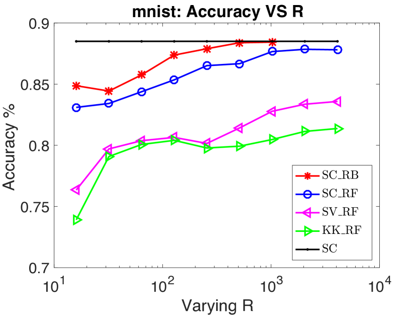
(a) Accuracy (Acc)

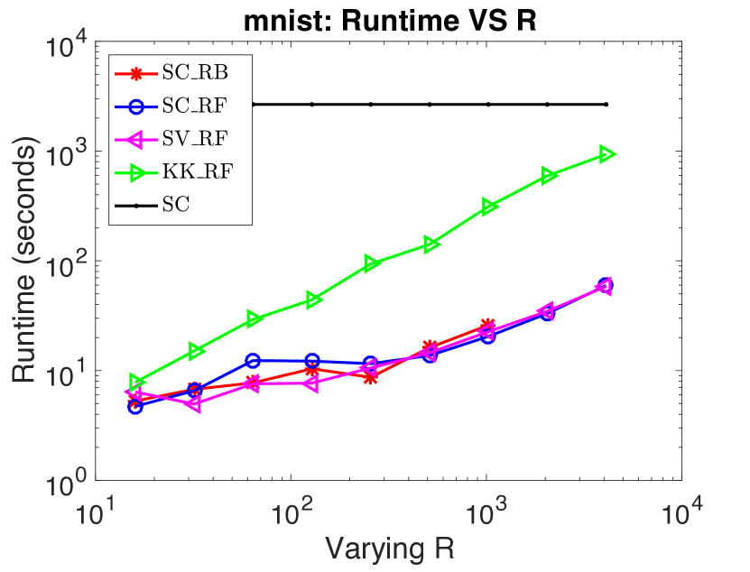
(b) Runtime

Figure 2. Clustering accuracy and runtime when varying $R$ on mnist for random features based SC methods.

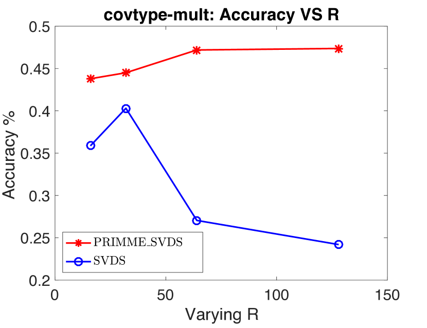
(a) Accuracy (Acc)

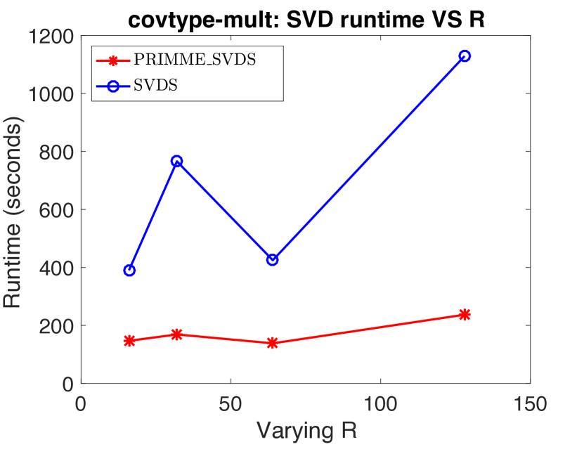
(b) Runtime

Figure 3. Clustering accuracy and runtime when varying $R$ on covtype-mult using PRIMME_SVDS and Matlab SVDS.

Setup. The first goal here is to investigate the scalability of SC_RB over the vanilla SC method in terms of runtime while achieving the similar performance. The second goal is to study the behavior of various scalable SC and approximate Kernel K-means methods based on different random features. We limit our comparisons among two random features (RF and RB) based SC or Kernel K-means type methods. We choose the mnist dataset since it has been widely studied for convergence analysis of approximation in the literature (Chitta et al., 2012; Chen and Cai, 2011; Li et al., 2016). We report runtime and commonly used Accuracy (Acc) as our measurement metric when varying the rank $R$ from 16 to 4096 (except SC_RB from 16 to 1024).

Results. We investigate how the performance of different methods changes when the number $R$ of random features (RF and RB) increases from 16 to 4096. Fig. 2(b) illustrates that despite a large sparse feature matrix generated by RB, the computational time of SC_RB is orders of magnitudes less expensive compared to that of exact SC, and is comparable to other SC methods based on RF features. This is the desired feature of SC_RB that it can achieve higher accuracy than other efficient SC methods without comprising the computation time. As shown in Fig. 2(a), we can see that the clustering accuracy (Acc) of all methods generally converge to that of exact SC but with different convergence rates. More importantly, SC_RB yields faster convergence compared to other scalable SC methods based on RF features, which confirms our analysis in Theorem 3. For instance, SC_RB with $R=1024$ has already reached the same accuracy as the exact SC method while SC_RF converges relatively slower to the exact SC and get close to SC with $R=4096$. Interestingly, SV_RF and KK_RF are not competitive in Accuracy, indicating that approximating the graph Laplacian matrix $L$ is more beneficial than these that approximating the similarity matrix $W$ in some cases.

5.3. Effects of SVD solvers on runtime

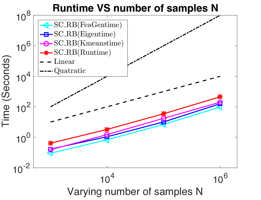
(a) Size of Poker (1M)

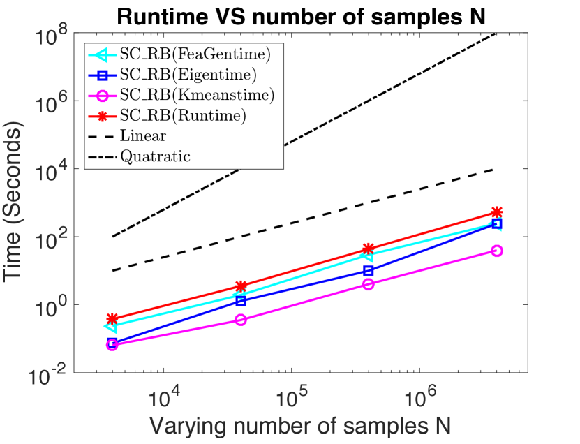
(b) Size of SUSY (4M)

Figure 4. Linear scalability of SC_RB when varying the number of samples $N$. Linear and quadratic complexity are also plotted for easy comparisons.

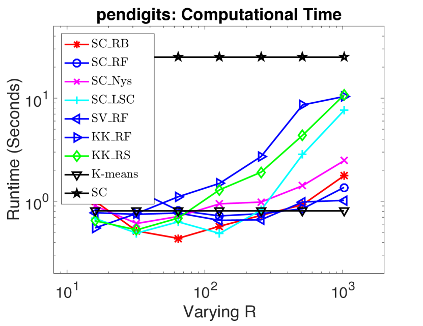
(a) pendigits

(b) letter

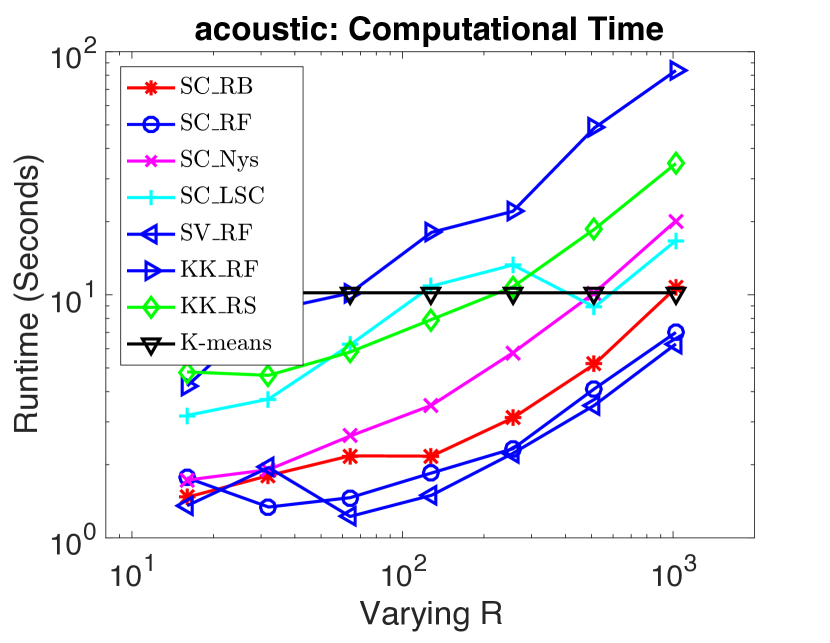
(c) acoustic

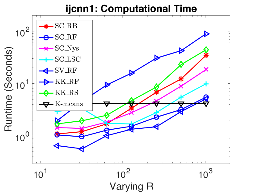
(d) ijcnn1

Figure 5. Scalability of SC_RB and other methods on 4 datasets when varying the number of latent features $R$.

Setup. We perform experiments to study the effects of various SVD solvers on runtime for SC_RB. We choose the covtype-mult dataset due to two reasons: 1) RB generates a very large sparse matrix $\mathbf{Z}$ having the size of half millions in the number of data points and tens of millions in the number of sparse features, which challenges any existing SVD solver in a single machine; 2) the convergence of iterative eigensolver largely depends on the well-separation of the desired eigenvalues. Unfortunately, the gap between the largest eigenvalues of covtype-mult is very small $O(1E-5)$, making it a difficult eigenvalue problem. We compare PRIMME_SVDS with Matlab SVDS function, a widely used SVD solver routine in the research community. We also set stopping tolerance 1E-5 to yield faster convergence for both solvers. We vary $R$ for SC_RB from 16 to 128 and record the Accuracy (Acc) and Runtime (in Seconds) as our performance metrics for this set of experiment.

Results. Fig. 3 shows how the accuracy (Acc) and runtime changes for SC_RB using these two different SVD solvers when varying the rank $R$ on covtype-mult dataset. Interestingly, SC_RB with PRIMME_SVDS delivers more consistent accuracy than that with SVDS. This may be because Matlab SVDS function has a difficult time to converge to multiple very close singular values, showing an warning message ”reach default maximum iterations”. However, as shown in Fig. 3(b), less accurate singular triplets (from Matlab SVDS) takes significantly more computational time compared to PRIMME_SVDS, especially when $R$ increases. In contrast, the computational time of eigendecomposition using PRIMME_SVDS changes slowly with increased $R$. Thanks to the power of PRIMME, the proposed SC_RB could achieve good clustering performance based on high-quality singular vectors while managing attractable computational time for very large sparse matrices.

5.4. Scalability of SC_RB when varying the number of data samples $N$

Setup. Our goal in this experiment is to assess the scalability of SC_RB when varying the number of data samples $N$ on poker dataset and another large dataset SUSY . We vary the number of data samples in the range of $N=[100\ \ 1,000,000]$ on poker and $N=[4000\ \ 4,000,000]$ on the synthetic dataset. We use the same hyperparameters as the previous experiments and fix $R=256$. Since RB can be easily parallelized, we accelerate its computation using 4 threads. Matlab also automatically parallelize the matrix-vector operations for other solvers. We report the runtime for generating random binning feature matrix, computing partial eigendecomposition using state-of-the-art eigensolver (Stathopoulos and McCombs, 2010; Wu et al., 2017), performing K-means, and the overall runtime, respectively.

Results. Figure 4 clearly shows that SC_RB indeed scales linearly with the increase in the number of data samples. Note that even for large datasets consisting of millions of samples, the computation time of SC_RB is still less than 500 seconds. These results suggest that: (i) SC_RB exhibits linear scalability in $N$ and is comtenant of handling large datasets in a reasonable time frame; (ii) with the state-of-the-art eigensolver (Wu et al., 2017), the complexity of computing a few of eigenvectors for spectral clustering is indeed linearly proportional to the matrix size $N$.

The key factor that contributes to the competitive computation time and linear scalability of SC_RB in the data size $N$ is that we take into account the end-to-end spectral clustering pipeline consisting of the build blocks, RB generation, eigensolver and K-means, and our approach ensures each component takes a similar (linear) computation complexity, as analyzed in Section 3.

5.5. Scalability of SC_RB when varying the number of RB features $R$

Setup. We further investigate the scalablity of various random-feature-based, sampling-based SC methods and approximate Kernel K-means methods when varying the latent feature size $R$. One of our goal is to investigate whether the latent matrix rank $R$ is linearly proportional to $N$. If this is true, then the total complexity of an approximation method is still bounded by $O(N^{2})$, which is an unfavorable property for large-scale data. Therefore, we study the computational time of 8 baselines when varying $R$ from 16 to 1024 on 4 datasets. The other settings are same as before.

Results. Figure 5 shows that the computation of SC_RB is as efficient as other approximation methods. There are several comments worth making here. First, compared to the quadratic complexity of exact SC in Figures 5(a) and 5(b), various approximation methods except KK_RF require much less computational time. It means that the total complexity of various methods are respecting to $O(NR)$ where $R$ could be somehow treated as a constant as long as $R$ is significantly smaller than $N$. Remarkably, Figures 5(c) and 5(d) show that most of approximation methods including SC_RB can even behave as efficient as K-means on the original dataset. Obviously, most of these methods exhibit clear linear relation with $R$, indicating that these methods are not tightly associated with $N$. In other words, if the low rank $R$ in any method is respecting with $N$, then the total complexity of the method is proportional to $O(N^{2})$, which should yield non-linear scalability respecting to $R$. The only exception is the KK_RF method, which consistently requires much more runtime compared to other methods, making it less attractable than other methods.

6. Conclusion

In this paper, we have presented a scalable end-to-end spectral clustering method based on RB features (SC_RB) for overcoming two computational bottlenecks - similarity graph construction and eigendecomposition of the graph Laplacian. By leveraging RB features, the pairwise similarity matrix can be approximated implicitly by the inner product of the RB feature matrix, which significantly reduces the computational complexity from quadratic to linear in terms of the number of data samples. We further show how to effectively and directly apply SVD on the weighted RB feature matrix and introduce a state-of-the-art sparse SVD solver to efficiently manage the SVD computation for a very large sparse matrix. Our theoretical analysis shows that by drawing $R$ grids with at least $\kappa$ number of non-empty bins per grid, SC_RB can guarantee convergence to exact spectral clustering with a rate of $O(1/(\kappa R))$ under the same pairwise graph construction process, which is much faster than other Random Features based SC methods. Our extensive experiments on 8 benchmarks over 4 performance metrics demonstrate that SC_RB either outperforms or matches 8 baselines in both accuracy and computational time, and corroborate that SC_RB indeed exhibits linear scalability in terms of the number of data samples and the number of RB features.

References

- (1)
- Bojchevski et al. (2017) Aleksandar Bojchevski, Yves Matkovic, and Stephan Günnemann. 2017. Robust Spectral Clustering for Noisy Data: Modeling Sparse Corruptions Improves Latent Embeddings. In ACM SIGKDD International Conference on Knowledge Discovery and Data Mining. 737–746.
- Chang and Lin (2011) Chih-Chung Chang and Chih-Jen Lin. 2011. LIBSVM: a library for support vector machines. ACM transactions on intelligent systems and technology (TIST) 2, 3 (2011), 27.
- Chen et al. (2006) Bo Chen, Bin Gao, Tie-Yan Liu, Yu-Fu Chen, and Wei-Ying Ma. 2006. Fast spectral clustering of data using sequential matrix compression. In European Conference on Machine Learning. Springer, 590–597.
- Chen et al. (2016) Jie Chen, Lingfei Wu, Kartik Audhkhasi, Brian Kingsbury, and Bhuvana Ramabhadrari. 2016. Efficient one-vs-one kernel ridge regression for speech recognition. In Acoustics, Speech and Signal Processing (ICASSP), 2016 IEEE International Conference on. IEEE, 2454–2458.
- Chen and Hero (2016) Pin-Yu Chen and Alfred O Hero. 2016. Phase transitions and a model order selection criterion for spectral graph clustering. arXiv preprint arXiv:1604.03159 (2016).
- Chen and Wu (2017) Pin-Yu Chen and Lingfei Wu. 2017. Revisiting Spectral Graph Clustering with Generative Community Models. In Data Mining (ICDM), 2017 IEEE International Conference on. IEEE, 51–60.
- Chen et al. (2018) Pin-Yu Chen, Baichuan Zhang, and Mohammad Al Hasan. 2018. Incremental eigenpair computation for graph Laplacian matrices: theory and applications. Social Network Analysis and Mining 8, 1 (2018), 4.
- Chen et al. (2011) Wen-Yen Chen, Yangqiu Song, Hongjie Bai, Chih-Jen Lin, and Edward Y Chang. 2011. Parallel spectral clustering in distributed systems. IEEE transactions on pattern analysis and machine intelligence 33, 3 (2011), 568–586.
- Chen and Cai (2011) Xinlei Chen and Deng Cai. 2011. Large Scale Spectral Clustering with Landmark-Based Representation.. In AAAI, Vol. 5. 14.
- Chitta et al. (2011) Radha Chitta, Rong Jin, Timothy C Havens, and Anil K Jain. 2011. Approximate kernel k-means: Solution to large scale kernel clustering. In Proceedings of the 17th ACM SIGKDD international conference on Knowledge discovery and data mining. ACM, 895–903.
- Chitta et al. (2012) Radha Chitta, Rong Jin, and Anil K Jain. 2012. Efficient kernel clustering using random fourier features. In Data Mining (ICDM), 2012 IEEE 12th International Conference on. IEEE, 161–170.
- Dhillon et al. (2004) Inderjit S Dhillon, Yuqiang Guan, and Brian Kulis. 2004. Kernel k-means: spectral clustering and normalized cuts. In Proceedings of the tenth ACM SIGKDD international conference on Knowledge discovery and data mining. ACM, 551–556.
- Fowlkes et al. (2004) Charless Fowlkes, Serge Belongie, Fan Chung, and Jitendra Malik. 2004. Spectral grouping using the Nyström method. IEEE transactions on pattern analysis and machine intelligence 26, 2 (2004), 214–225.
- Gittens et al. (2013) Alex Gittens, Prabhanjan Kambadur, and Christos Boutsidis. 2013. Approximate spectral clustering via randomized sketching. Ebay/IBM Research Technical Report (2013).
- Hartigan and Wong (1979) John A Hartigan and Manchek A Wong. 1979. Algorithm AS 136: A k-means clustering algorithm. Journal of the Royal Statistical Society. Series C (Applied Statistics) 28, 1 (1979), 100–108.
- Li et al. (2016) Yeqing Li, Junzhou Huang, and Wei Liu. 2016. Scalable Sequential Spectral Clustering.. In AAAI. 1809–1815.
- Lin and Cohen (2010) Frank Lin and William W Cohen. 2010. Power iteration clustering. In Proceedings of the 27th international conference on machine learning (ICML-10). 655–662.
- Liu et al. (2013) Jialu Liu, Chi Wang, Marina Danilevsky, and Jiawei Han. 2013. Large-scale spectral clustering on graphs. In Proceedings of the Twenty-Third international joint conference on Artificial Intelligence. AAAI Press, 1486–1492.
- Liu et al. (2007) Tie-Yan Liu, Huai-Yuan Yang, Xin Zheng, Tao Qin, and Wei-Ying Ma. 2007. Fast large-scale spectral clustering by sequential shrinkage optimization. Advances in Information Retrieval (2007), 319–330.
- Liu et al. (2010) Wei Liu, Junfeng He, and Shih-Fu Chang. 2010. Large graph construction for scalable semi-supervised learning. In Proceedings of the 27th international conference on machine learning (ICML-10). 679–686.
- Ng et al. (2002) Andrew Y Ng, Michael I Jordan, and Yair Weiss. 2002. On spectral clustering: Analysis and an algorithm. In Advances in neural information processing systems. 849–856.
- Rahimi and Recht (2008) Ali Rahimi and Benjamin Recht. 2008. Random features for large-scale kernel machines. In Advances in neural information processing systems. 1177–1184.
- Sakai and Imiya (2009) Tomoya Sakai and Atsushi Imiya. 2009. Fast Spectral Clustering with Random Projection and Sampling.. In MLDM. Springer, 372–384.
- Shi and Malik (2000) Jianbo Shi and Jitendra Malik. 2000. Normalized cuts and image segmentation. IEEE Transactions on pattern analysis and machine intelligence 22, 8 (2000), 888–905.
- Shinnou and Sasaki (2008) Hiroyuki Shinnou and Minoru Sasaki. 2008. Spectral Clustering for a Large Data Set by Reducing the Similarity Matrix Size.. In LREC.
- Stathopoulos and McCombs (2010) Andreas Stathopoulos and James R McCombs. 2010. PRIMME: preconditioned iterative multimethod eigensolver—methods and software description. ACM Transactions on Mathematical Software (TOMS) 37, 2 (2010), 21.
- Tremblay et al. (2016) Nicolas Tremblay, Gilles Puy, Rémi Gribonval, and Pierre Vandergheynst. 2016. Compressive spectral clustering. In International Conference on Machine Learning. 1002–1011.
- Von Luxburg (2007) Ulrike Von Luxburg. 2007. A tutorial on spectral clustering. Statistics and computing 17, 4 (2007), 395–416.
- Williams and Seeger (2001) Christopher KI Williams and Matthias Seeger. 2001. Using the Nyström method to speed up kernel machines. In Advances in neural information processing systems. 682–688.
- Wu et al. (2017) Lingfei Wu, Eloy Romero, and Andreas Stathopoulos. 2017. PRIMME_SVDS: A high-performance preconditioned SVD solver for accurate large-scale computations. SIAM Journal on Scientific Computing 39, 5 (2017), S248–S271.
- Wu and Stathopoulos (2015) Lingfei Wu and Andreas Stathopoulos. 2015. A preconditioned hybrid svd method for accurately computing singular triplets of large matrices. SIAM Journal on Scientific Computing 37, 5 (2015), S365–S388.
- Wu et al. (2016) Lingfei Wu, Ian EH Yen, Jie Chen, and Rui Yan. 2016. Revisiting random binning features: Fast convergence and strong parallelizability. In Proceedings of the 22nd ACM SIGKDD International Conference on Knowledge Discovery and Data Mining. ACM, 1265–1274.
- Wu et al. (2018a) Lingfei Wu, Ian En-Hsu Yen, Fangli Xu, Pradeep Ravikuma, and Michael Witbrock. 2018a. D2KE: From Distance to Kernel and Embedding. arXiv preprint arXiv:1802.04956 (2018).
- Wu et al. (2018b) Lingfei Wu, Ian En-Hsu Yen, Jinfeng Yi, Fangli Xu, Qi Lei, and Michael Witbrock. 2018b. Random Warping Series: A Random Features Method for Time-Series Embedding. In International Conference on Artificial Intelligence and Statistics. 793–802.
- Yan et al. (2009) Donghui Yan, Ling Huang, and Michael I Jordan. 2009. Fast approximate spectral clustering. In Proceedings of the 15th ACM SIGKDD international conference on Knowledge discovery and data mining. ACM, 907–916.
- Yang and Leskovec (2015) Jaewon Yang and Jure Leskovec. 2015. Defining and evaluating network communities based on ground-truth. Knowledge and Information Systems 42, 1 (2015), 181–213.
- Yen et al. (2014) Ian En-Hsu Yen, Ting-Wei Lin, Shou-De Lin, Pradeep K Ravikumar, and Inderjit S Dhillon. 2014. Sparse random feature algorithm as coordinate descent in hilbert space. In Advances in Neural Information Processing Systems. 2456–2464.
- Zaki et al. (2014) Mohammed J Zaki, Wagner Meira Jr, and Wagner Meira. 2014. Data mining and analysis: fundamental concepts and algorithms. Cambridge University Press.