Physics of Pair Producing Gaps in Black Hole Magnetospheres

Abstract

In some low-luminosity accreting supermassive black hole systems, the supply of plasma in the funnel region can be a problem. It is believed that a local region with unscreened electric field can exist in the black hole magnetosphere, accelerating particles and producing high energy gamma-rays that can create $e^{\pm}$ pairs. We carry out time-dependent self-consistent 1D PIC simulations of this process, including inverse Compton scattering and photon tracking. We find a highly time-dependent solution where a macroscopic gap opens quasi-periodically to create $e^{\pm}$ pairs and high energy radiation. If this gap is operating at the base of the jet in M87, we expect an intermittency on the order of a few $r_{g}/c$, which coincides with the time scale of the observed TeV flares from the same object. For Sagittarius A* the gap electric field can potentially grow to change the global magnetospheric structure, which may explain the lack of a radio jet at the center of our galaxy.

1 Introduction

Black holes can be powerful engines for active galactic nuclei (AGN), galactic superluminal sources, gamma-ray bursts, and other energetic phenomena. It has been shown that the rotational energy of a Kerr black hole can be electromagnetically extracted to launch powerful jets (Blandford & Znajek, 1977; McKinney et al., 2012). However, the process relies on the field being frozen into the plasma, and if matter from the accretion disk cannot easily cross the field line to enter the jet, some mechanism of plasma supply in the jet funnel is needed (e.g., Blandford & Znajek, 1977; Beskin et al., 1992; Hirotani & Okamoto, 1998).

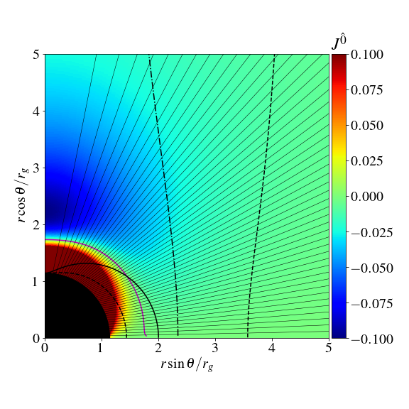
Figure 1: Force-free split monopole solution around a Kerr black hole with spin $a=0.99$, in Boyer-Lindquist coordinates. The color map shows the charge density $J^{\hat{0}}$ as measured by ZAMO. Thin black lines—contours of the flux function $\Psi$; black solid line—ergosphere; black dashed lines—light surfaces; black dash-dotted line—stagnation surface; magenta line—$J^{\hat{0}}=0$.

Consider a nearly force-free, steady monopolar magnetosphere around a Kerr black hole (Figure 1). Particles moving in the strong magnetic field with Larmor radius $r_{L}\ll r_{g}\equiv GM/c^{2}$ slide along the field line like beads on a wire. Because of the existence of two light surfaces, particles are flung outward to infinity through the outer light surface and flung inward towards the event horizon through the inner light surface. In between there is a stagnation surface, located at the maximum of an effective potential. The nature of the particle motion indicates that even if the magnetosphere is initially filled with plasma, particles will inevitably leak out from the two light surfaces. When the plasma density becomes too low to conduct the current required by a force-free magnetosphere, the rotation induced electric field will have a parallel component that cannot be screened, forming a gap and accelerating particles to high enough energies, which then produce high energy photons through inverse Compton (IC) or synchrotron/curvature processes and initiate a pair cascade that replenishes the plasma, restoring the magnetosphere to near force-free.

The charge and current densities required to maintain a force-free magnetosphere have a few important properties for the monopole solution: (1) the poloidal current is constant along the flux tube; (2) the 4-current is spacelike everywhere; (3) there exists a null surface where the zero angular momentum observer(ZAMO) measured charge density $J^{\hat{0}}=0$ (Figure 1). The null surface has been regarded as a point of separation of the plasma since if $J^{\hat{k}}$ has the same sign as the slope of $J^{\hat{0}}$, and the plasma is charge-separated, then the current is conducted by opposite charges moving away from the null surface, opening a vacuum region where parallel electric field can grow (e.g. Cheng et al., 1986; Beskin et al., 1992; Hirotani & Okamoto, 1998). Meanwhile, the stagnation surface has also been considered to be a place for the gap to form (Broderick & Tchekhovskoy, 2015). Whether there is a preferred gap location has yet to be tested using kinetic simulations.

The magnetospheric gap has also been invoked to explain the fast $\gamma$-ray variability observed from some AGN (Levinson & Rieger, 2011; Aleksić et al., 2014; Broderick & Tchekhovskoy, 2015; Aharonian et al., 2017; Katsoulakos & Rieger, 2018). However, so far in the literature the gap physics has been treated based on over-simplified vacuum models. In this work, we will focus on the low luminosity regime (such that MeV photons from the disk are not enough to produce the necessary charges), and study the microphysics and dynamics of the gap using radiative PIC simulations.

2 Numerical setup

We would like to model the physical system described in section 1 using the simplest physics possible while capturing all the salient features, namely the existence of a null surface, a stagnation point, and two light surfaces. Spacetime correction to the equations of motion for particles and fields are responsible for these effects, while the magnitude of these corrections are actually small compared with the electromagnetic forces. Therefore we model the flux tube using a flat space model while trying to capture these features using different means.

In the flat spacetime model, we simply have 1D Maxwell equations (e.g., Chen & Beloborodov, 2013; Timokhin & Arons, 2013):

$$\frac{\partial E_{r}}{\partial t}=4\pi(j_{B}-j_{r}),\qquad\frac{\partial E_{r}}{\partial r}=4\pi(\rho-\rho_{\mathrm{co}}).$$ (1)

where we take the background $j_{B}$ to be constant and use a spatial profile of $\rho_{\mathrm{co}}$ similar to the GR background charge density. See the third row of Figure 2 for the background charge and current density profiles.

We include the effect of the light surfaces in 1D using a model inspired by the light cylinder effect of a rotating neutron star. Consider the classic Michel monopole solution (Michel, 1973):

$$\boldsymbol{B}=\frac{\mu}{r^{2}}\,\hat{\boldsymbol{r}}+B_{\phi}\,\hat{\boldsymbol{\phi}},\quad B_{\phi}=-\frac{\Omega r\sin\theta}{c}B_{r}=\beta_{\phi}B_{r}.$$ (2)

The field lines form an Archimedean spiral and become mostly toroidal outside the light cylinder where $\Omega r\sin\theta=c$, or $\beta_{\phi}=-1$. The field line rotates at an angular velocity of $\Omega$, and for any particles outside the light cylinder, the corotation velocity is superluminal. The particle compensates by sliding along the field line outwards; the total velocity is always less than $c$.

We can easily derive the equation for the 1D constrained motion of a particle along a monopolar field line:

$$\frac{dp_{r}}{dt} =mc\frac{\beta_{\phi}\Omega\sin\theta}{\gamma}\left(\frac{\gamma-p_{r}/mc}{1+\beta_{\phi}^{2}}\right)^{2}+qE_{r},$$ (3)

$$\frac{dr}{dt} =v_{r}=c\frac{p_{r}/\gamma mc+\beta_{\phi}^{2}}{1+\beta_{\phi}^{2}},$$ (4)

where $p_{r}$ is the canonical momentum and

$$\gamma=\sqrt{(p_{r}/mc)^{2}+1+\beta_{\phi}^{2}}$$ (5)

is the Lorentz factor of the particle. One can immediately see that no matter the value of $p_{r}$, $|p_{r}/\gamma mc|<1$, so when $\beta_{\phi}^{2}\geq 1$, $v_{r}>0$ and the particle is only allowed to move in one direction. In our numerical simulations we model the light surfaces in exactly the same way. We assume a profile for $\beta_{\phi}$ that is linear and antisymmetric across the center of the simulation box, reaching $\pm 1$ at the light surfaces which are located at 0.05 and 0.95 of the simulation box. This way the inner light surface is simply a mirror of the outer light surface; the mid point of the box will be our “stagnation surface”.

We use a simplified version of the code Aperture developed by the author Alex Chen as a part of his PhD thesis (Chen, 2017). The code only evolves the 1D equations listed above, but keeping the charge-conserving current deposit scheme proposed by Esirkepov (2001). This ensures that Gauss’s law is satisfied at all times if it is satisfied initially, so we only need to evolve the first of equation (1). Comparison between background and numerical values of $\rho$ and $j$ in the third row of Figure 2 confirms excellent charge conservation over time.

2.1 Choice of units and scales

In our flat spacetime model we take the background current density $j_{B}$ to be constant, which naturally defines a plasma frequency and skin depth:

$$\omega_{p}=\sqrt{\frac{4\pi ej_{B}}{mc}},\qquad\lambda_{p}=\frac{c}{\omega_{p}}.$$ (6)

Thus we measure time using $\omega_{p}^{-1}$ and length using $\lambda_{p}$. Also choosing $j_{B}$ as the unit of current, the electric field will be measured by

$$E_{0}=\frac{4\pi j_{B}}{\omega_{p}},\qquad\frac{eE_{0}\lambda_{p}}{mc^{2}}=1.$$ (7)

which simply means that $\tilde{E}=1$ corresponds to a voltage drop of $mc^{2}$ over a single $\lambda_{p}$, where the tilde denotes a dimensionless quantity. In this set of units, naturally we have the unit of energy being $mc^{2}$ and momentum being $mc$. We define pair multiplicity as $\mathcal{M}=(n_{+}+n_{-})ec/j_{B}$.

The profile of $\rho_{\mathrm{co}}$ adds another parameter since it varies on the length scale of $r_{g}$. The computational domain needs to accommodate several $r_{g}$ since we would like to include both light surfaces. For the physical systems we are interested in, e.g. M87, $\lambda_{p}/r_{g}$ is on the order of $10^{-8}$ (Table 1). It is extremely difficult to have such scale separation in a PIC simulation. Therefore we rescale this ratio, keeping $r_{g}\gg\lambda_{p}$, and develop a semi-analytical model to infer what would happen at physical parameters.

2.2 Mechanism for pair production

The dominant mechanism for pair production in the black hole magnetosphere is the collision of high energy photons with the low-energy photons from the disk. The high energy photons come mostly from IC scattering of the background soft photons by energetic leptons. We carry out the full radiative transfer including IC scattering and the subsequent photon-photon collision assuming both happen on the same background photon field. We assume a soft photon spectral distribution of $I(\epsilon)=\epsilon dN/d\epsilon=I_{0}(\epsilon/\epsilon_{\mathrm{min}})^{-\alpha}$ which cuts off at $\epsilon_{\mathrm{min}}$ and extends up to $\sim 0.1$ MeV. We use the Monte Carlo method to sample the photon energy from a single IC event, then compute its free path by drawing from an exponential distribution with a mean $\ell_{\gamma\gamma}$. We track this photon until it is converted to an $e^{\pm}$ pair at the end of its free path. When the photon is not energetic enough to convert within the box, we do not track it, but still cool the particle as if it emitted the photon.

The mean free path $\ell_{\gamma\gamma}$ is energy dependent. The smallest mean free path occurs when $\tilde{E}_{\mathrm{ph}}\tilde{\epsilon}_{\mathrm{min}}\sim 2$ where $\ell_{\gamma\gamma}\approx 5\ell_{\mathrm{IC}}$, and $\ell_{\mathrm{IC}}$ is the characteristic IC mean free path in Thomson regime, $\ell_{\mathrm{IC}}=1/n_{s}\sigma_{T}=\alpha/I_{0}\sigma_{T}$. For lower photon energy, $\ell_{\gamma\gamma}$ increases:

$$\ell_{\gamma\gamma}(E_{\mathrm{ph}})\approx 5\ell_{\mathrm{IC}}\left(\frac{\tilde{E}_{\mathrm{ph}}\tilde{\epsilon}_{\mathrm{min}}}{2}\right)^{-\alpha}$$ (8)

The modeling of the IC process introduces several new numerical parameters: the spectral index $\alpha$, the peak soft photon energy $\epsilon_{\mathrm{min}}$, and a characteristic free path for IC scattering $\ell_{\mathrm{IC}}$. $\epsilon_{\mathrm{min}}$ sets the energy scale of the discharge, while $\ell_{\mathrm{IC}}$ puts a new length scale into the problem. The inferred characteristic values of these parameters are listed in Table 1. In our rescaling of the problem we focus on the optically thick regime, and ensure parameter ordering $\lambda_{p}\ll\ell_{\mathrm{IC}}\ll r_{g}$.

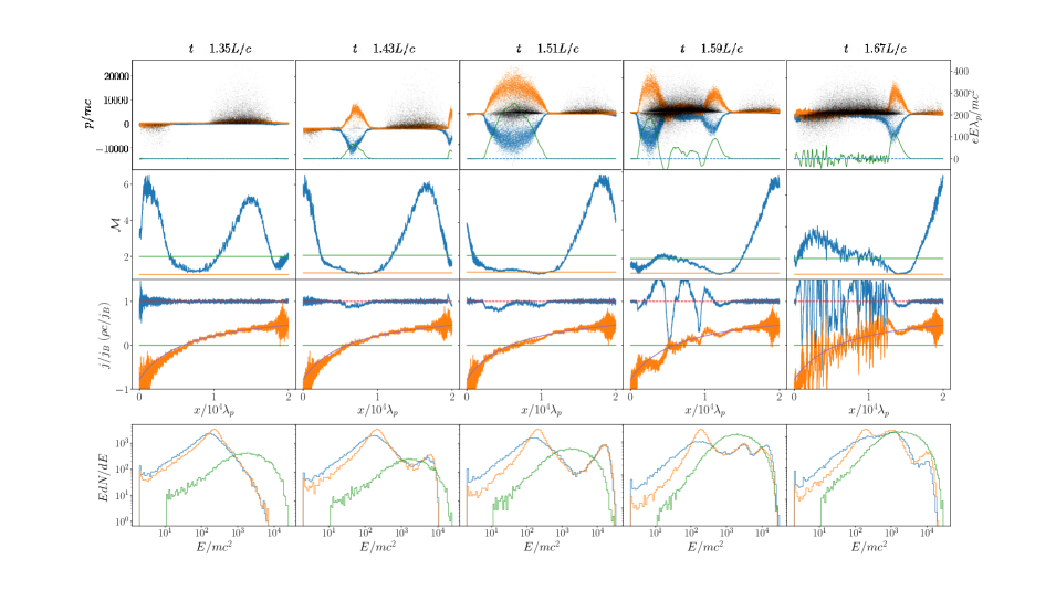
Figure 2: Time evolution of the gap. From left to right are snapshots at labeled times, where $L$ is the size of the box. The 4 panels from top to bottom are: 1) Phase space plots for electrons (blue), positrons (orange), and photons (black). The green line is electric field and its scale is on the right. 2) Pair multiplicity $\mathcal{M}$. Orange and green lines mark $\mathcal{M}=1$ and $2$ respectively. 3) Current $j$ (blue) and charge density $\rho$ (orange) and their background values. 4) Spectrum of electrons (blue), positrons (orange), and photons (green).

3 Time-dependent gap in 1D

3.1 Simulation results

We start from a plasma-filled initial condition where $E=0$ and $\rho=\rho_{\mathrm{co}}$. The initial pair multiplicity is 2, and all particles start at rest. Initially small plasma-scale electric field develops to help the current to flow, but since the box is leaky on both ends, plasma multiplicity drops over time. This happens fastest where $d\rho_{\mathrm{co}}/dx$ is largest. When $\mathcal{M}\lesssim 1$, an electric gap opens locally to accelerate particles to high Lorentz factors, and subsequently initiate pair creation, screening this gap, and launching macroscopic bunches of pair plasma to both directions. Screening of the electric field creates oscillations similar to those described by Levinson et al. (2005). Eventually when the pairs are advected out of the light surfaces and multiplicity drops again, the same cycle is initiated. In the full length of one simulation, we are able to see several cycles of the gap formation. We also tried starting with a vacuum electric field, but obtained the same solution.

Figure 2 shows one such gap cycle, where we used $\alpha=1.2$, $\ell_{\mathrm{IC}}=10\lambda_{p}$, $r_{g}/\lambda_{p}\sim 10^{4}$, and $\tilde{\epsilon}_{\mathrm{min}}=10^{-6}$. It is the third time the gap develops in the simulation. As multiplicity drops from the previous cycle of pair creation, the system tries to maintain a macroscopic region as large as possible with $\mathcal{M}\gtrsim 1$ by drawing plasma from the side. When plasma flow can not sustain this state, a gap opens quickly over the whole region where $\mathcal{M}\sim 1$. As a result, in all our simulations the gap size $h\sim r_{g}$, and depends weakly on all parameters. The gap shown develops around the null surface, but it is not a guaranteed feature. It tends to develop wherever local multiplicity drops below unity, which can be anywhere due to plasma flow and delayed conversion of photons.

The photon spectrum shown in Figure 2 is not to be confused with the observable one. Due to limits of computational power, we only track photons that convert to pairs within the box, so the shown spectrum should be interpreted more as an absorption spectrum. In fact, most of the dissipated power in the gap goes into radiation that leaves the box, only a small fraction of it converting into $e^{\pm}$ pairs. The peak multiplicity from the gap is usually $\mathcal{M}\sim 10$.

There are two well-defined spectral peaks for the particle energy shown in Figure 2. When the gap is screened, the low energy peak is a spectral break where the IC cooling becomes ineffective, $\ell_{\mathrm{cool,IC}}\sim L$. When the gap is open, another spectral peak arises at higher energy. These are the primary particles accelerated in the gap, and the peak energy $\gamma_{p}$ is controlled by the gap electric field and IC cooling.

3.2 Physics of the gap

Consider a region in the magnetosphere where plasma multiplicity $\mathcal{M}=1$ and $j=j_{B}$ at $t=0$. Electrons and positrons have to be counter streaming at speed of light to provide the current, so the number density of each species evolves as

$$n_{\pm}(x,t)=\frac{j_{B}\pm\rho_{\mathrm{co}}(x\mp ct)c}{2ec},$$ (9)

Assuming $\rho_{\mathrm{co}}$ varies linearly across this region with a slope $k=d\rho_{\mathrm{co}}/dx\sim j_{B}/r_{g}c$, we see that the current decreases over time if $kj_{B}>0$:

$$j(t)=en_{+}(x,t)c+en_{-}(x,t)c\approx j_{B}-kc^{2}t.$$ (10)

In particular, the time scale for the decrease of current depends on the spatial scale over which $\rho_{\mathrm{co}}$ varies. As a result, the electric field at the center of the gap increases as $t^{2}$

$$E_{\parallel}=\frac{1}{2}kc^{2}t^{2}.$$ (11)

The gap starts to be screened when enough photons emitted by the primary particles convert to pairs within the gap. During the characteristic time $t$, a primary particle goes through a number of

$$N(\epsilon)=\frac{ct}{\ell_{\mathrm{IC}}}\left(\frac{\epsilon}{\epsilon_{\mathrm{min}}}\right)^{-\alpha}$$ (12)

scatterings with target photons of energy $\epsilon$ ($\geq\epsilon_{\mathrm{min}}$), generating $\gamma$-rays at energy $E_{\rm ph}=2\gamma_{p}^{2}\epsilon$ (applicable when $\gamma_{p}\tilde{\epsilon}\lesssim 0.1$). Among these $\gamma$-rays, a number of $\kappa$ convert to pairs within time $t$:

$$\kappa=N(\epsilon)\frac{ct}{\ell_{\gamma\gamma}(E_{\rm ph})}=\frac{c^{2}t^{2}}{5\ell_{\mathrm{IC}}^{2}}\left(\gamma_{p}^{2}\tilde{\epsilon}_{\mathrm{min}}^{2}\right)^{\alpha},$$ (13)

which turns out to be independent of $\epsilon$. For the gap to be screened, $\kappa$ needs to be on the order of $1-10$ (we find that $\kappa\sim 10$ reproduces well the results of our production runs). For most parameter regimes of interest, when the screening happens the primary particles have short enough cooling lengths such that the electrostatic acceleration is balanced by the IC loss, so $\gamma_{p}$ is determined by $E_{\parallel}$ through

$$eE_{\parallel}=\frac{4}{3}\gamma_{p}^{2}\frac{\alpha}{\alpha-1}\frac{\epsilon_{\mathrm{min}}}{\ell_{\mathrm{IC}}}.$$ (14)

Using Equations (11)(13)(14), we can then obtain the peak electric field

$$\frac{E_{\parallel}}{E_{0}}=\left(\frac{5\kappa\ell_{\mathrm{IC}}^{2}}{8\pi\lambda_{p}r_{g}}\left(\frac{3(\alpha-1)}{4\alpha}\frac{\ell_{\mathrm{IC}}}{\lambda_{p}}\tilde{\epsilon}_{\mathrm{min}}\right)^{-\alpha}\right)^{\frac{1}{\alpha+1}},$$ (15)

and $\gamma_{p}$ can be calculated from Equation (14). From $E_{\parallel}$, and gap size $h\sim r_{g}$, we can estimate the maximum gap power

$$L_{\rm gap}\sim E_{\parallel}j_{B}r_{g}^{3}\sim\frac{E_{\parallel}}{B}L_{\rm jet}.$$ (16)

We expect most of this power to be radiated away in gamma-rays.

Figure 3 shows that for all runs below the Klein-Nishina regime, there is good agreement between the analytical model and the measured scaling from the simulations. However, the above calculation no longer holds well if primary particle energy approaches the Klein-Nishina regime: $\gamma_{p}\gtrsim 0.1/\tilde{\epsilon}_{\mathrm{min}}$, which happens at relatively small optical depth $\tau_{0}=r_{g}/\ell_{\mathrm{IC}}\lesssim$ a few hundred. In that case, IC cooling becomes less efficient and our argument for radiation balanced acceleration breaks down. We expect $\gamma_{p}$ and the gap power to be much higher than our model would predict, which is what we see in the simulations. The gaps in this regime tend to be larger, but are still screened quasi-periodically as long as $\tau_{0}>$ a few.

In the limit where $\ell_{\mathrm{IC}}\gtrsim r_{g}$ or $\tau_{0}\lesssim 1$, we found that it is increasingly difficult to screen the gap, which develops to encompass the whole domain. Particles are accelerated into deep Klein-Nishina regime where $\gamma_{p}\gg 1/\tilde{\epsilon}_{\mathrm{min}}$, and $E_{\parallel}\gtrsim B$. In this limit we expect significant changes of the magnetospheric structure due to the gap, possibly killing the jet structure, and 1D approximation we employed in this paper is no longer appropriate.

3.3 Scaling to real systems

Table 1: Parameters for M87 and Sgr A*

	M87	Sgr A*
$M\;(M_{\odot})$	$6.6\times 10^{9}$	$(4.3\pm 0.4)\times 10^{6}$
$r_{g}\;({\rm cm})$	$10^{15}$	$6.4\times 10^{11}$
$L_{s}/L_{\rm Edd}$	$10^{-6}$	$10^{-9}$
$B$ (G)	200	30
$n_{\rm GJ}\;({\rm cm}^{-3})$	$5\times 10^{-4}$	$0.1$
$\lambda_{p}/r_{g}$	$2\times 10^{-8}$	$2.6\times 10^{-6}$
$u_{s}\;({\rm erg\,cm^{-3}})$	0.1	0.15
$n_{s}\;({\rm cm^{-3}})$	$10^{13}$	$2\times 10^{13}$
$\epsilon_{\mathrm{min}}$ (meV)	1.2	1.2
$\epsilon_{\mathrm{min}}/m_{e}c^{2}$	$2.3\times 10^{-9}$	$2.3\times 10^{-9}$
$\alpha$	1.2	1.25
$\ell_{\mathrm{IC}}/r_{g}$	$1.5\times 10^{-4}$	$0.12$
$E_{\parallel}/E_{0}$	$1.8\times 10^{3}$	$2.9\times 10^{4}$
$E_{\parallel}/B$	$3.6\times 10^{-5}$	0.075
$\gamma_{p}$	$2.7\times 10^{7}$	$3\times 10^{8}$
$L_{\rm gap}\;({\rm erg\,s^{-1}})$	$3.6\times 10^{39}$	$4\times 10^{34}$

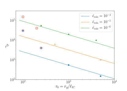
Figure 3: Scaling of primary particle Lorentz factor $\gamma_{p}$ with optical depth and soft photon peak $\epsilon_{\mathrm{min}}$. Lines are our analytical predictions (equations (14) and (15)). Triangles, crosses, and dots are runs with $\tilde{\epsilon}_{\mathrm{min}}=10^{-6}$, $10^{-5}$, $10^{-4}$ respectively, and should be compared with corresponding colored lines. All simulations are run with $\alpha=1.2$ and $r_{g}/\lambda_{p}=10^{4}$. The red-circled points are above $0.1/\tilde{\epsilon}_{\mathrm{min}}$, close to Klein-Nishina regime, and our analytical model is no longer applicable.

The most relevant systems where the spark gap might exist are low luminosity AGN like M87 and Sgr A*. We list the physical parameters inferred from observation in Table 1, as well as predictions from our physical model. The observational parameters are based on Broderick & Tchekhovskoy (2015). For M87 we expect it to be well described by our model, and indeed the predicted $\gamma_{p}\sim 3\times 10^{7}$ is well below the KN regime. The typical gamma-ray photons that are produced by these primary particles will be in the range of $0.1$ to a few TeV; most of them will escape the outer light surface. This coincides with the observed energy range of the TeV flares from M87 (Abramowski et al., 2012). Our time-dependent gap model also predicts time variability of several $r_{g}/c$, which for M87 would be about $\sim$day, again coinciding with the observed time scale of the flares. However, the total gap power predicted by our model is at best only consistent with the quiescent state, and too low for the flares. Whether this mechanism can explain the origin of M87 flares will be investigated in a future paper.

For Sgr A* however, $\gamma_{p}>0.1/\tilde{\epsilon}_{\mathrm{min}}$, and we are in the Klein-Nishina regime. In this case we expect the actual primary particle energy to be higher, and $L_{\mathrm{gap}}$ might become comparable to $L_{\mathrm{jet}}$. As a result, the simplistic 1D approximation we adopted in this paper is no longer applicable, as this gap should be able to significantly affect the global magnetosphere structure. This potentially can explain the lack of an apparent jet structure from the center of our galaxy. To properly treat this regime a global magnetospheric simulation will be needed.

4 Discussion

We have presented self-consistent 1D simulations of pair cascade in a magnetized plasma within the black hole magnetosphere. Informed by the numerical results we developed a semi-analytical model for the electric gap, providing an estimate for gap power in systems that are optically thick to inverse Compton scattering.

Traditionally the study of the discharge problem in the BH magnetosphere were often based on a vacuum gap model around the null surface, drawing analogy to the outer gap model in pulsar magnetospheres (e.g. Ptitsyna & Neronov, 2016; Ford et al., 2017). We have shown through numerical simulations that the physical conditions for such models are never realized: the domain never tolerates a local vacuum region, nor a static gap. Electric field develops to accelerate leptons as soon as the local multiplicity drops below unity, initiating the process of pair discharge. Moreover, the gap can develop anywhere depending on plasma flow, not necessarily at the null surface.

We did not include the GR correction to the particle equations of motion. Instead, the GR effect is entirely captured by the varying background charge density $\rho_{\mathrm{co}}$, and the presence of an inner light surface. Without GR both features will be absent. We think this is an appropriate simplification that allows us to focus on the electrodynamics and microphysics. A proper general relativistic set of equations could in principle be implemented, as was recently done by Levinson & Cerutti (2018). However, they report an overall quasi-steady state which is different from what we observe. We believe the main differences are the treatment of light surfaces, and they focus on a low optical depth regime $r_{g}/\ell_{\mathrm{IC}}\lesssim 10$. The logical extension of the results in this paper is to look at how the global structure of the magnetosphere will interact with the gap, especially when the gap power becomes comparable to the jet power.

References

- Abramowski et al. (2012) Abramowski, A., Acero, F., Aharonian, F., et al. 2012, ApJ, 746, 151
- Aharonian et al. (2017) Aharonian, F. A., Barkov, M. V., & Khangulyan, D. 2017, ApJ, 841, 61
- Aleksić et al. (2014) Aleksić, J., Ansoldi, S., Antonelli, L. A., et al. 2014, Science, 346, 1080
- Beskin et al. (1992) Beskin, V. S., Istomin, Y. N., & Parev, V. I. 1992, Soviet Ast., 36, 642
- Blandford & Znajek (1977) Blandford, R. D., & Znajek, R. L. 1977, MNRAS, 179, 433
- Broderick & Tchekhovskoy (2015) Broderick, A. E., & Tchekhovskoy, A. 2015, ApJ, 809, 97
- Chen (2017) Chen, A. Y. 2017, PhD thesis, Columbia University
- Chen & Beloborodov (2013) Chen, A. Y., & Beloborodov, A. M. 2013, ApJ, 762, 76
- Cheng et al. (1986) Cheng, K. S., Ho, C., & Ruderman, M. 1986, ApJ, 300, 500
- Esirkepov (2001) Esirkepov, T. Z. 2001, Computer Physics Communications, 135, 144
- Ford et al. (2017) Ford, A. L., Keenan, B. D., & Medvedev, M. V. 2017, ArXiv e-prints, arXiv:1706.00542 [astro-ph.HE]
- Hirotani & Okamoto (1998) Hirotani, K., & Okamoto, I. 1998, ApJ, 497, 563
- Katsoulakos & Rieger (2018) Katsoulakos, G., & Rieger, F. M. 2018, ApJ, 852, 112
- Levinson & Cerutti (2018) Levinson, A., & Cerutti, B. 2018, ArXiv e-prints, arXiv:1803.04427 [astro-ph.HE]
- Levinson et al. (2005) Levinson, A., Melrose, D., Judge, A., & Luo, Q. 2005, ApJ, 631, 456
- Levinson & Rieger (2011) Levinson, A., & Rieger, F. 2011, ApJ, 730, 123
- McKinney et al. (2012) McKinney, J. C., Tchekhovskoy, A., & Blandford, R. D. 2012, MNRAS, 423, 3083
- Michel (1973) Michel, F. C. 1973, ApJ, 180, L133
- Ptitsyna & Neronov (2016) Ptitsyna, K., & Neronov, A. 2016, A&A, 593, A8
- Timokhin & Arons (2013) Timokhin, A. N., & Arons, J. 2013, MNRAS, 429, 20