Abstract

This paper investigates a novel algorithmic approach to data representation based on kernel methods. Assuming that the observations lie in a Hilbert space $\mathcal{X}$, the introduced Kernel Autoencoder (KAE) is the composition of mappings from vector-valued Reproducing Kernel Hilbert Spaces (vv-RKHSs) that minimizes the expected reconstruction error. Beyond a first extension of the auto-encoding scheme to possibly infinite dimensional Hilbert spaces, KAE further allows to autoencode any kind of data by choosing $\mathcal{X}$ to be itself a RKHS. A theoretical analysis of the model is carried out, providing a generalization bound, and shedding light on its connection with Kernel Principal Component Analysis. The proposed algorithms are then detailed at length: they crucially rely on the form taken by the minimizers, revealed by a dedicated Representer Theorem. Finally, numerical experiments on both simulated data and real labeled graphs (molecules) provide empirical evidence of the KAE performances.

1 INTRODUCTION

As experienced by any practitioner, data representation is critical to the application of Machine Learning, whatever the targeted task, supervised or unsupervised. An answer to this issue consists in feature engineering, a step that requires time-consuming interactions with domain experts. To overcome these limitations, Representation Learning (RL) (Bengio et al.,, 2013) aims at building automatically new features in an unsupervised fashion. Recent applications to neural nets pre-training, image denoising and semantic hashing have renewed a strong interest in RL, now a proper research field. Among successful RL approaches, mention has to be made of Autoencoders (AEs) (Vincent et al.,, 2010), and their generative variant, Deep Boltzman Machines (Salakhutdinov and Hinton,, 2009).

AEs attempt to learn a pair of encoding/decoding functions under structural constraints so as to capture the most important properties of the data (Alain and Bengio,, 2014). If they have mostly been studied under the angle of neural networks (Baldi,, 2012) and deep architectures (Vincent et al.,, 2010), the concepts underlying AEs are very general and go beyond neural implementations. In this work, we develop a general framework inspired from AEs, and based on Operator-Valued Kernels (OVKs) (Senkene and Tempel’man,, 1973) and vector-valued Reproducing Kernel Hilbert Spaces (vv-RKHSs). Mainly developed for supervised learning, OVKs provide a nonparametric way to tackle complex output prediction problems (Álvarez et al.,, 2012), including multi-task regression, structured output prediction (Brouard et al., 2016b, ), or functional regression (Kadri et al.,, 2016). This work is a first contribution to combine OVKs with AEs, enlarging the latters’ applicability scope - so far restricted to $\mathbb{R}^{d}$ - to any data described by a similarity matrix.

We start from the simplest formulation in which a Kernel Autoencoder (KAE) is a pair of encoding/decoding functions lying in two different vv-RKHSs, and whose composition approximates the identity function. This approach is further extended to a general framework involving the composition of an arbitrary number of mappings, defined and valued on Hilbert spaces. A crucial application of KAEs arises if the input space is itself a RKHS: it allows to perform autoencoding on any type of data, by first mapping it to the RKHS, and then applying a KAE. The solutions computation, even in infinite dimensional spaces, is made possible by a Representer Theorem and the use of the kernel trick. This unlocks new applications on structured objects for which feature vectors are missing or too complex (e.g. in chemoinformatics).

Kernelizing an AE criterion has also been proposed by Gholami and Hajisami, (2016). But their approach differs from ours in many key aspects: it is restricted to AEs with 2 layers and composed of linear maps only; it relies on semi-supervised information; it comes with no theoretical analysis, and within a hashing perspective solely. Despite a similar title, the work by Kampffmeyer et al., (2017) has no connection with ours. Authors use standard AEs, and regularize the learning by aligning the latent code with some predetermined feature map. In the experimental section, we implement autoencoding on graphs, which cannot be done by means of standard AEs. Graph AEs (Kipf and Welling,, 2016) do not autoencode graphs, but $\mathbb{R}^{d}$ points with an additive graph characterizing the data structure.

The rest of the article is structured as follows. The novel kernel-based framework for RL is detailed in Section 2. A generalization bound and a strong connection with Kernel PCA are established in Section 3, whereas Section 4 describes the algorithmic approach based on a Representer Theorem. Illustrative numerical experiments are displayed in Section 5, while concluding remarks are collected in Section 6. Finally, technical details are deferred to the Supplementary Material.

2 THE KERNEL AUTOENCODER

In this section, we introduce a general framework for building AEs based on vv-RKHSs. Here and throughout the paper, the set of bounded linear operators mapping a vector space $E$ to itself is denoted by $\mathcal{L}(E)$, and the set of mappings from a set $A$ to an ensemble $B$ by $\mathcal{F}(A,B)$. The adjoint of an operator $M$ is denoted by $M^{*}$. Finally, $\llbracket n\rrbracket$ denotes the set $\{1,\ldots,n\}$ for any integer $n\in\mathbb{N}^{*}$.

2.1 Background on vv-RKHSs

Vv-RKHSs allow to cope with the approximation of functions from an input set $\mathcal{X}$ to some output Hilbert space $\mathcal{Y}$ (Senkene and Tempel’man,, 1973; Caponnetto et al.,, 2008). Vv-RKHS can be defined from an OVK, which extends the classic notion of positive definite kernel. An OVK is a function $\mathcal{K}\colon\mathcal{X}\times\mathcal{X}\to\mathcal{L}(\mathcal{Y})$, that satisfies the following two properties (Micchelli and Pontil,, 2005):

$$\forall(x,x^{\prime})\in\mathcal{X}\times\mathcal{X},\qquad\mathcal{K}(x,x^{\prime})=\mathcal{K}(x^{\prime},x)^{*},$$

and $\forall n\in\mathbb{N}^{*},\forall~{}\{(x_{i},y_{i})\}_{1\leq i\leq n}\in(\mathcal{X}\times\mathcal{Y})^{n},$

$$\sum_{1\leq i,j\leq n}\langle y_{i},\mathcal{K}(x_{i},x_{j})y_{j}\rangle_{\mathcal{Y}}\geq 0.$$

A simple example of OVK is the separable kernel such that: $\forall~{}(x,x^{\prime})\in\mathcal{X}\times\mathcal{X},$ $\mathcal{K}(x,x^{\prime})=k(x,x^{\prime})A$, where $k$ is a positive definite scalar-valued kernel, and $A$ is a positive semi-definite operator on $\mathcal{Y}$. Its relevance for multi-task learning has been highlighted for instance by Micchelli and Pontil, (2005).

Let $\mathcal{K}$ be an OVK, and for $x\in\mathcal{X}$, let $K_{x}\colon y\in\mathcal{Y}\mapsto K_{x}y\in\mathcal{F}(X,Y)$ the linear operator such that:

$$\forall x^{\prime}\in\mathcal{X},~{}(K_{x}y)(x^{\prime})=\mathcal{K}(x^{\prime},x)y.$$

Then, there is a unique Hilbert space $\mathcal{H}_{\mathcal{K}}\subset\mathcal{F}(\mathcal{X},\mathcal{Y})$ called the vv-RKHS associated to $\mathcal{K}$, with inner product $\langle\cdot,\cdot\rangle_{\mathcal{H}_{\mathcal{K}}}$ and norm $\lVert\cdot\rVert_{\mathcal{H}_{\mathcal{K}}}$, such that $\forall x\in\mathcal{X}$:

• $K_{x}$ spans the space $\mathcal{H}_{K}$ ($\forall y\in\mathcal{Y}\colon K_{x}y\in\mathcal{H}_{K}$)

• $K_{x}$ is bounded for the uniform norm

• $\forall f\in\mathcal{H},~{}f(x)=K_{x}^{*}f$ (i.e. reproducing property)

2.2 Input Output Kernel Regression

Now, let us assume that the output space $\mathcal{Y}$ is chosen itself as a RKHS, say $\mathcal{H}$, associated to the positive definite scalar-valued kernel $k:\mathcal{Z}\times\mathcal{Z}\to\mathbb{R}$, with $\mathcal{Z}$ a non-empty set. Working in the vv-RKHS $\mathcal{H}_{\mathcal{K}}$ associated to an OVK $\mathcal{K}:\mathcal{X}\times\mathcal{X}\to\mathcal{L}(\mathcal{H})$ opens the door to a large family of learning tasks where the output set $\mathcal{Z}$ can be a set of complex objects such as nodes in a graph, graphs (Brouard et al., 2016a, ) or functions (Kadri et al.,, 2016). Following the work of Brouard et al., 2016b , we refer to these methods as Input Output Kernel Regression (IOKR). IOKR has been shown to be of special interest in case of Ridge Regression, where closed-form solutions are available besides classical gradient descent algorithms. Note that in a general supervised setting, learning a function $f\in\mathcal{H}_{\mathcal{K}}$ is not sufficient to provide a prediction in the output set, and a pre-image problem has to be solved. In sections 2.5 and 4.3, a similar idea is applied at the last layer of our KAE, allowing for auto-encoding non-vectorial data while avoiding complex pre-image problems.

2.3 The 2-layer Kernel Autoencoder (KAE)

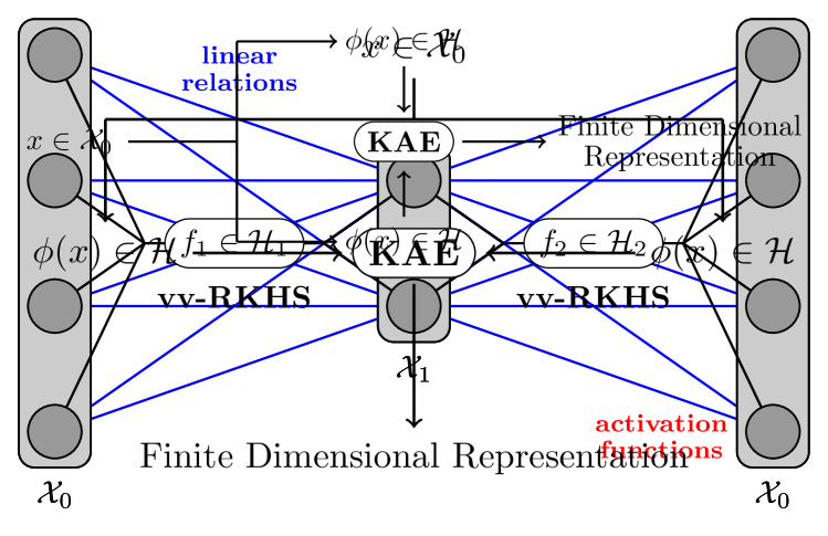
Figure 1: Standard and Kernel 2-layer Autoencoders

Let $S=(x_{1},\;\ldots,\;x_{n})$ denote a sample of $n$ independent realizations of a random vector $X$, valued in a separable Hilbert space $(\mathcal{X}_{0},\;\|\cdot\|_{\mathcal{X}_{0}})$ with unknown probability distribution $P$, and such that there exists $M<+\infty,\|X\|_{\mathcal{X}_{0}}\leq M$ almost surely. On the basis of the training sample $S$, we are interested in constructing a pair of encoding/decoding mappings $\left(f:\mathcal{X}_{0}\rightarrow\mathcal{X}_{1},\;g:\mathcal{X}_{1}\rightarrow\mathcal{X}_{0}\right)$, where $(\mathcal{X}_{1},\;\|\cdot\|_{\mathcal{X}_{1}})$ is the (Hilbert) representation space. Just as for standard AEs, we regard as good internal representations the ones that allow for an accurate recovery of the original information in expectation. The problem to be solved states as follows:

$$\min_{\begin{subarray}{c}(f,g)\in\mathcal{H}_{1}\times\mathcal{H}_{2}\\ \|f\|_{\mathcal{H}_{1}}\leq s,~{}\|g\|_{\mathcal{H}_{2}}\leq t\end{subarray}}\epsilon(f,g)\coloneqq\mathbb{E}_{X\sim P}\left\|X-g\circ f(X)\right\|^{2}_{\mathcal{X}_{0}},$$ (1)

where $\mathcal{H}_{1}$ and $\mathcal{H}_{2}$ are two vv-RKHSs, and $s$ and $t$ two positive constants. $\mathcal{H}_{1}$ is associated to an OVK $\mathcal{K}_{1}:\mathcal{X}_{0}\times\mathcal{X}_{0}\rightarrow\mathcal{L}(\mathcal{X}_{1})$, while $\mathcal{H}_{2}$ is associated to $\mathcal{K}_{2}:\mathcal{X}_{1}\times\mathcal{X}_{1}\rightarrow\mathcal{L}(\mathcal{X}_{0})$. Figure 1 illustrates the parallel and differences between standard and kernel 2-layer Autoencoders.

Following the Empirical Risk Minimization (ERM) paradigm, the true risk (1) is replaced by its empirical version

$$\hat{\epsilon}_{n}(f,g)\coloneqq\frac{1}{n}\sum_{i=1}^{n}||x_{i}-g\circ f(x_{i})||^{2}_{\mathcal{X}_{0}},$$ (2)

and a penalty term $\Omega(f,g)\coloneqq\lambda\|f\|_{\mathcal{H}_{1}}^{2}+\mu\|g\|_{\mathcal{H}_{2}}^{2}$ is added instead of the norm constraints (see Theorem 1). Solutions to the following regularized ERM problem shall be referred to as 2-layer KAE:

$$\min_{(f,g)\in\mathcal{H}_{1}\times\mathcal{H}_{2}}\hat{\epsilon}_{n}(f,g)+\Omega(f,g).$$ (3)

2.4 The Multi-layer KAE

Like for standard AEs, the model previously described can be directly extended to more than 2 layers. Let $L\geq 3$, and consider a collection of Hilbert spaces $\mathcal{X}_{0},\;\ldots,\;\mathcal{X}_{L}$, with $\mathcal{X}_{L}=\mathcal{X}_{0}$. For $0\leq l\leq L-1$, the space $\mathcal{X}_{l}$ is supposed to be endowed with an OVK $\mathcal{K}_{l+1}:\mathcal{X}_{l}\times\mathcal{X}_{l}\rightarrow\mathcal{L}\left(\mathcal{X}_{l+1}\right)$, associated to a vv-RKHS $\mathcal{H}_{l+1}\subset\mathcal{F}(\mathcal{X}_{l},\mathcal{X}_{l+1})$. We then want to minimize $\epsilon(f_{1},\ldots,f_{L})$ over $\prod_{l=1}^{L}\mathcal{H}_{l}$. Setting $\Omega(f_{1},\ldots,f_{L})\coloneqq\sum_{l=1}^{L}\lambda_{l}\|f_{l}\|_{\mathcal{H}_{L}}^{2}$ allows for a direct extension of (3):

$$\min_{f_{l}\in\mathcal{H}_{l}}~{}\frac{1}{n}\sum_{i=1}^{n}\left\|x_{i}-f_{L}\circ\ldots\circ f_{1}(x_{i})\right\|^{2}_{\mathcal{X}_{0}}+\sum_{l=1}^{L}\lambda_{l}\|f_{l}\|_{\mathcal{H}_{l}}^{2}.$$ (4)

2.5 The General Hilbert KAE and the $\text{K}^{2}$AE

Figure 2: Autoencoding any data thanks to $\text{K}^{2}$AE

So far, and up to the regularization term, the main difference between standard and kernel AEs is the function space on which the reconstruction criterion is optimized: respectively neural functions or RKHS ones. But what should also be highlighted is that RKHS functions are valued in general Hilbert spaces, while neural functions are restricted to $\mathbb{R}^{d}$. As shall be seen in section 4.3, this enables KAEs to handle data from infinite dimensional Hilbert spaces (e.g. function spaces), what standard AEs are unable to do. To our knowledge, this first extension of the autoencoding scheme is novel.

But even more interesting is the possible extension when the input/output Hilbert space is chosen to be itself a RKHS. Indeed, let $\mathcal{X}_{0}$ denote now any set (without the Hilbert assumption). In the spirit of IOKR, let us first map $x\in\mathcal{X}_{0}$ to the RKHS $\mathcal{H}$ associated to some scalar kernel $k$, and its canonical feature map $\phi$. Since the $\phi(x_{i})^{\prime}s$ are by definition valued in a Hilbert, KAE can be applied. This way, we have extended the autoencoding paradigm to any set, and finite dimensional representations can be extracted from all types of data. Again, such extension is novel to our knowledge. Figure 2 depicts the procedure, referred to as $\text{K}^{2}$AE, since the new criterion is a kernelization of the KAE that reads:

$$\frac{1}{n}\sum_{i=1}^{n}\left\|\phi(x_{i})-f_{L}\circ\ldots\circ f_{1}(\phi(x_{i}))\right\|^{2}_{\mathcal{H}}+\sum_{l=1}^{L}\lambda_{l}\|f_{l}\|_{\mathcal{H}_{l}}^{2}.$$ (5)

3 THEORETICAL ANALYSIS

It is the purpose of this section to investigate theoretical properties of the introduced model, its capacity to be learnt from training data with a controlled generalization error, and the connection between $\text{K}^{2}$AE and Kernel PCA (KPCA) namely.

3.1 Generalization Bound

While the algorithmic formulation aims at minimizing the regularized risk (3), the subsequent theoretical analysis focuses on the constrained problem (1). Theorem 1 relates the solutions from the two approaches to each other, so that bounds derived in the latter setting also apply to numerical solutions of the first one.

Theorem 1.

Let $V:\mathcal{H}_{1}\times\ldots\times\mathcal{H}_{L}\rightarrow\mathbb{R}$ be an arbitrary function. Consider the two problems:

$$\min_{f_{l}\in\mathcal{H}_{l}}~{}\left\{V(f_{1},\ldots,f_{L})+\sum_{l=1}^{L}\lambda_{l}\|f_{l}\|_{\mathcal{H}_{l}}^{2}\right\},$$ (6)

$$\min_{\begin{subarray}{c}f_{l}\in\mathcal{H}_{l}\\ \|f_{l}\|_{\mathcal{H}_{l}}\leq s_{l}\end{subarray}}~{}V(f_{1},\ldots,f_{L}).$$ (7)

Then, for any $(\lambda_{1},\;\ldots,\;\lambda_{L})\in\mathbb{R}_{+}^{L}$, there exists $(s_{1},\;\ldots,\;s_{L})\in\mathbb{R}_{+}^{L}$ such that any (respectively, local) solution to problem (6) is also a (respectively, local) solution to problem (7).

Refer to Section A.1 for the proof and a discussion on the converse statement.

In order to establish generalization bound results for empirical minimizers in the present setting, we now define two key quantities involved in the proof, i.e. Rademacher and Gaussian averages for classes of Hilbert-valued functions.

Definition 2.

Let $\mathcal{X}$ be any measurable space, and $H$ a separable Hilbert space. Consider a class $\mathcal{C}$ of measurable functions $h:\mathcal{X}\rightarrow H$. Let $\bm{\sigma}_{1},\;\ldots,\;\bm{\sigma}_{n}$ be $n\geq 1$ independent $H$-valued Rademacher variables and define:

$$\widehat{\mathscr{R}}_{n}(\mathcal{C}(S))=\mathbb{E}_{\bm{\sigma}}\left[\sup_{h\in\mathcal{C}}\frac{1}{n}\sum_{i=1}^{n}\left\langle\bm{\sigma}_{i},h(x_{i})\right\rangle_{H}\right].$$

If $H=\mathbb{R}$, it is the classical Rademacher average (see e.g. Mohri et al., (2012) p.34), while, when $H=\mathbb{R}^{p}$, it corresponds to the expectation of the supremum of the sum of the Rademacher averages over the $p$ components of $h$ (see Definition 2.1 in Maurer and Pontil, (2016)). If $H$ is an infinite dimensional Hilbert space with countable orthonormal basis $(e_{k})_{k\in\mathbb{N}}$, we have:

$$\widehat{\mathscr{R}}_{n}(\mathcal{C}(S))=\mathbb{E}_{\bm{\sigma}}\left[\sup_{h\in\mathcal{C}}\frac{1}{n}\sum_{i=1}^{n}\sum_{k=1}^{\infty}\sigma_{i,k}\left\langle h(x_{i}),e_{k}\right\rangle_{H}\right].$$

The Gaussian counterpart of $\widehat{\mathscr{R}}_{n}(\mathcal{C}(S))$, obtained by replacing Rademacher random variables/processes with standard $H$-valued Gaussian ones, is denoted by $\widehat{\mathscr{G}}_{n}(\mathcal{C}(S))$ throughout the paper.

For the sake of simplicity, results in the rest of the subsection are derived in the 2-layer case solely, with $\mathcal{X}_{1}$ finite dimensional (i.e. $\mathcal{X}_{1}=\mathbb{R}^{p}$), although the approach remains valid for deeper architectures.

Let $\mathcal{H}_{1,s}\coloneqq\left\{f\in\mathcal{H}_{1}:\|f\|_{\mathcal{H}_{1}}\leq s\right\}$, and similarly $\mathcal{H}_{2,t}\coloneqq\left\{g\in\mathcal{H}_{2}:\|g\|_{\mathcal{H}_{2}}\leq t,\sup_{y\in\mathbb{R}^{p}}\|g(y)\|_{\mathcal{X}_{0}}\leq M\right\}$. We shall use the notation $\mathcal{H}_{s,t}\subset\mathcal{F}(\mathcal{X}_{0},\mathcal{X}_{0})$ to mean the space of composed functions $\mathcal{H}_{1,s}\circ\mathcal{H}_{2,t}\coloneqq\left\{h\in\mathcal{F}(\mathcal{X}_{0},\mathcal{X}_{0}):\exists(f,g)\in\mathcal{H}_{1,s}\times\mathcal{H}_{2,t},~{}h=g\circ f\right\}$. To simplify the notation, $\epsilon$ (and $\hat{\epsilon}_{n}$) may be abusively considered as a functional with one or two arguments: $\epsilon(f,g)=\epsilon(g\circ f)=\mathbb{E}_{X\sim P}\left\|X-g\circ f(X)\right\|_{\mathcal{X}_{0}}^{2}$. Finally, let $\hat{h}_{n}$ denote the minimizer of $\hat{\epsilon}_{n}$ over $\mathcal{H}_{s,t}$, and $\epsilon^{*}$ the infimum of $\epsilon$ on the same functional space.

Assumption 3.

There exists $K<+\infty$ such that:

$$\forall x\in\mathcal{X}_{0},\;\;\text{{Tr}}\big{(}\mathcal{K}_{1}(x,x)\big{)}\leq Kp.$$

Assumption 4.

There exists $L<+\infty$ such that for all $y,\;y^{\prime}$ in $\mathbb{R}^{p}$:

$$\text{{Tr}}\big{(}\mathcal{K}_{2}(y,y)-2\mathcal{K}_{2}(y,y^{\prime})+\mathcal{K}_{2}(y^{\prime},y^{\prime})\big{)}\leq L^{2}~{}\|y-y^{\prime}\|_{\mathbb{R}^{p}}^{2}.$$

Theorem 5.

Let $\mathcal{K}_{1}$ and $\mathcal{K}_{2}$ be OVKs satisfying Assumptions 3 and 4 respectively. Then, there exists a universal constant $C_{0}<+\infty$ such that, for any $0<\delta<1$, we have with probability at least $1-\delta$:

$$\epsilon(\hat{h}_{n})-\epsilon^{*}\leq C_{0}LMst\sqrt{\frac{Kp}{n}}+24M^{2}\sqrt{\frac{\log(2)/\delta}{2n}}.$$

The proof relies on a Rademacher bound, which is in turn upper bounded using Corollary 4 in Maurer, (2016), an extension of Theorem 2 in Maurer, (2014) proved in the Supplementary Material, and several intermediary results derived from the stipulated assumptions. Technical details are deferred to Section A.2.

Attention should be paid to the fact that constants in Theorem 5 appear in a very interpretable fashion: the less spread the input (the smaller the constant $M$), the more restrictive the constraints on the functions (the smaller $K$, $L$, $s$ and $t$), and the smaller the internal dimension $p$, the sharper the bound.

3.2 $\text{K}^{2}$AE and Kernel PCA: a Connection

Just as Bourlard and Kamp, (1988) have shown a mere equivalence between PCA and standard 2-layer AEs, a similar link can be established between 2-layer $\text{K}^{2}$AE and Kernel PCA (Schölkopf et al.,, 1997, 1998). Throughout the analysis, a 2-layer $\text{K}^{2}$AE is considered, with decomposable kernels made of linear scalar kernels and identity operators. Also, there is no penalization (i.e. $\lambda_{1}=\lambda_{2}=0$). We want to autoencode data into $\mathbb{R}^{p}$, after a first embedding through the feature map $\phi$, like in (5).

3.2.1 Finite Dimensional Feature Map

Let us assume first that $\phi$ is valued in $\mathbb{R}^{d}$, with $p<d<n$. Let $\Phi=(\phi(x_{1}),\ldots,\phi(x_{n}))^{\top}\in\mathbb{R}^{n\times d}$ denote the matrix storing the $\phi(x_{i})^{\top}$ to autoencode in rows. Note that $K_{\phi}=\Phi\Phi^{\top}\in\mathbb{R}^{n\times n}$ corresponds to the Gram matrix associated to $\phi$. As shall be seen in Theorem 6, the optimal $f$ and $g$ have a specific form, so that they only depend on two coefficient matrices, $A\in\mathbb{R}^{n\times p}$ and $B\in\mathbb{R}^{n\times d}$ respectively. Equipped with this notation, one has: $Y=f_{A}(\Phi)=\Phi\Phi^{\top}A\in\mathbb{R}^{n\times p}$, and $\widetilde{\Phi}=g_{B}(Y)=YY^{\top}B\in\mathbb{R}^{n\times d}$. Without penalization, the goal is then to minimize in $A$ and $B$:

$$\|\Phi-\widetilde{\Phi}\|_{\text{Fr}}^{2}.$$ (8)

$\widetilde{\Phi}$ being at most of rank $p$, we know from Eckart-Young Theorem that the best possible $\widetilde{\Phi}$ is given by $\Phi^{*}=U\Sigma_{p}V^{\top}$, where $\left(U\in\mathbb{R}^{n\times d},\Sigma\in\mathbb{R}^{d\times d},V^{\top}\in\mathbb{R}^{d\times d}\right)$ is the thin Singular Value Decomposition (SVD) of $\Phi$ such that $\Phi=U\Sigma V^{\top}$, and $\Sigma_{p}$ is equal to $\Sigma$, but with the $d-p$ smallest singular values zeroed.

Let us now prove that there exists a couple of matrices $(A^{*},B^{*})$ such that $g_{B^{*}}\circ f_{A^{*}}(\Phi)=\Phi^{*}$. One can verify that $(A^{*}=U_{p}{\overline{\Sigma}_{p}}^{-3/2},B^{*}=UV^{\top})$, with $U_{p}\in\mathbb{R}^{n\times p}$ storing only the $p$ largest eigenvectors of $K_{\phi}$, and $\overline{\Sigma}_{p}\in\mathbb{R}^{p\times p}$ the $p\times p$ top left block of $\Sigma_{p}$, satisfy it. Finally, the optimal encoding returned is $Y^{*}=f_{A^{*}}(\Phi)=\left(\sqrt{\sigma_{1}}u_{1},\ldots,\sqrt{\sigma_{p}}u_{p}\right)$, with $u_{1},\ldots,u_{p}$ the $p$ largest eigenvectors of $K_{\phi}$, while the KPCA’s new representation is $\left(\sigma_{1}u_{1},\ldots,\sigma_{p}u_{p}\right)$. Precisely, this $1/\sqrt{\sigma_{i}}$ rescaling may be seen as a KPCA whitening, and the encoding returned by KAE is actually known as the Kernel PCA Map (see e.g. Section 2.2.6 in Smola and Schölkopf, (1998)). Notice also that the algorithmic resolution of Problem (8) under different structural constraints (low rank assumption, sparsity) is studied in Smola and Schölkopf, (2000).

We have shown that a specific instance of $\text{K}^{2}$AE can be solved explicitly using a SVD, and that the optimal coding returned is close to the one output by KPCA.

3.2.2 Infinite Dimensional Feature Map

Let us assume now that $\phi$ is valued in a general Hilbert space $\mathcal{H}$. $\Phi$ is now seen as the linear operator from $\mathcal{H}$ to $\mathbb{R}^{n}$ such that $\forall\alpha\in\mathcal{H},~{}\Phi\alpha=\left(\left\langle\alpha,\phi(x_{1})\right\rangle_{\mathcal{H}},\ldots,\left\langle\alpha,\phi(x_{n})\right\rangle_{\mathcal{H}}\right)\in\mathbb{R}^{n}$. Since Theorem 1 makes no assumption on the dimensionality, everything stated in the finite dimensional scenario applies, except that $B\in\mathcal{L}(\mathcal{H},\mathbb{R}^{n})$, and that we minimize the Hilbert-Schmidt norm: $\|\Phi-\widetilde{\Phi}\|_{HS}^{2}$. We then need an equivalent of Eckart-Young Theorem. It still holds since its proof only requires the existence of an SVD for any operator, which is granted in our case since we deal with compact operators (they have finite rank $n$). The end of the proof is analogous to the finite dimensional case.

4 THE KAE ALGORITHMS

This section describes at length the algorithms we propose to solve problems (4) and (5). They raise two major issues as their objective functions are non-convex, and their search spaces are infinite dimensional. However, this last difficulty is solved by Theorem 6.

4.1 A Representer Theorem

Theorem 6.

Let $L_{0}\in\llbracket L\rrbracket$, and $V:\mathcal{X}_{L_{0}}^{n}\times\mathbb{R}_{+}^{L_{0}}\rightarrow\mathbb{R}$ a function of $n+L_{0}$ variables, strictly increasing in each of its $L_{0}$ last arguments. Suppose that $(f_{1}^{*},\ldots,f_{L_{0}}^{*})$ is a solution to the optimization problem:

$$\min_{f_{l}\in\mathcal{H}_{l}}V\Big{(} (f_{L_{0}}\circ\ldots\circ f_{1})(x_{1}),\ldots,(f_{L_{0}}\circ\ldots\circ f_{1})(x_{n}),$$

$$\left\|f_{1}\right\|_{\mathcal{H}_{1}},\ldots,\left\|f_{L_{0}}\right\|_{\mathcal{H}_{L_{0}}}\Big{)}.$$

Let ${x_{i}^{*}}^{(l)}\coloneqq f_{l}^{*}\circ\ldots\circ f_{1}^{*}(x_{i})$, with ${x_{i}^{*}}^{(0)}\coloneqq x_{i}$. Then, $\exists\left(\varphi_{1,1}^{*},\ldots,\varphi_{1,n}^{*},\ldots,\varphi_{L_{0},n}^{*}\right)\in\mathcal{X}_{1}^{n}\times\ldots\times\mathcal{X}_{L_{0}}^{n}:$

$$\forall~{}l\in\llbracket L_{0}\rrbracket,\quad f_{l}^{*}(\cdot)=\sum_{i=1}^{n}\mathcal{K}_{l}\left(~{}\cdot~{},{x_{i}^{*}}^{(l-1)}\right)\varphi_{l,i}^{*}.$$

Proof.

Refer to Section A.3 ∎

This Theorem exhibits a very specific structure for the minimizers, as each layer’s support vectors are the images of the original points by the previous layer.

4.2 Finite Dimension Case

In this section, let us assume that $\mathcal{X}_{l}=\mathbb{R}^{d_{l}}$ for $l\in\llbracket L\rrbracket$. The objective function of (4), viewed as a function of $(f_{L}\circ\ldots\circ f_{1})(x_{1}),\ldots,(f_{L}\circ\ldots\circ f_{1})(x_{n}),\|f_{1}\|_{\mathcal{H}_{1}},\ldots,\|f_{L}\|_{\mathcal{H}_{L}}$ satisfies the condition on $V$ involved in Theorem 6. After applying it (with $L_{0}=L$), problem (4) boils down to the problem of finding the $\varphi_{l,i}^{*}$’s, which are finite dimensional. This crucial observation shows that our problem can be solved in a computable manner. However, its convexity still cannot be ensured (see Section A.4).

The objective only depending on the $\varphi_{l,i}$’s, problem (4) can be approximately solved by Gradient Descent (GD). We now specify the gradient derivation in the decomposable OVKs case, i.e. for any layer $l$ there exists a scalar kernel $k_{l}$ and $A_{l}\in\mathcal{L}(X_{l})$ positive semidefinite such that $\mathcal{K}_{l}(x,x^{\prime})=k_{l}(x,x^{\prime})A_{l}$. All detailed computations can be found in Appendix B. Let $\Phi_{l}\coloneqq(\varphi_{l,1},\ldots,\varphi_{l,n})^{\top}\in\mathbb{R}^{n\times d_{l}}$ storing the coefficients $\varphi_{l,i}$ in rows, and $K_{l}\in\mathbb{R}^{n\times n}$ such that $\left[K_{l}\right]_{i,i^{\prime}}=k_{l}\Big{(}x_{i}^{(l-1)},x_{i^{\prime}}^{(l-1)}\Big{)}$. Let $(l_{0},i_{0})\in\llbracket L\rrbracket\times\llbracket n\rrbracket$, the gradient of the distortion term reads:

$$\Bigg{(}\nabla_{\varphi_{l_{0},i_{0}}} ~{}\frac{1}{n}\sum_{i=1}^{n}\|x_{i}-f_{L}\circ\ldots\circ f_{1}(x_{i})\|_{\mathcal{X}_{0}}^{2}\Bigg{)}^{\top}$$ (9)

$$= ~{}-\frac{2}{n}\sum_{i=1}^{n}\left(x_{i}-{x_{i}}^{(L)}\right)^{\top}\textbf{Jac}_{{x_{i}}^{(L)}}(\varphi_{l_{0},i_{0}}).$$

On the other hand, $\|f_{l}\|_{\mathcal{H}_{l}}^{2}$ may be rewritten as:

$$\|f_{l}\|_{\mathcal{H}_{l}}^{2}=\sum_{i,i^{\prime}=1}^{n}k_{l}\left({x_{i}}^{(l-1)},{x_{i^{\prime}}}^{(l-1)}\right)\left\langle\varphi_{l,i},A_{l}\varphi_{l,i^{\prime}}\right\rangle_{\mathcal{X}_{l}},$$ (10)

so that it may depend on $\varphi_{l_{0},i_{0}}$ in two ways: 1) if $l_{0}=l$, there is a direct dependence of the second quadratic term, 2) but note also that for $l_{0}<l$, the $\varphi_{l_{0},i}$ have an influence on the ${x_{i}}^{(l-1)}$ and so on the first term. This remark leads to the following formulas:

$$\nabla_{\Phi_{l}}~{}\|f_{l}\|_{\mathcal{H}_{l}}^{2}=2~{}K_{l}\Phi_{l}A_{l},$$ (11)

with $\nabla_{\Phi_{l}}F\coloneqq\left((\nabla_{\varphi_{l,1}}F)^{\top},\dots,(\nabla_{\varphi_{l,n}}F)^{\top}\right)^{\top}\in\mathbb{R}^{n\times d_{l}}$ storing the gradients of any real-valued function $F$ with respect to the $\varphi_{l,i}$ in rows. And when $l_{0}<l$:

$$\Big{(}\nabla_{\varphi_{l_{0},i_{0}}}\|f_{l}\|_{\mathcal{H}_{l}}^{2}\Big{)}^{\top}=2\sum_{i,i^{\prime}=1}^{n}\bigg{\{}$$ (12)

$$[N_{l}]_{i,i^{\prime}}\left(\nabla^{(1)}k_{l}\left({x_{i}}^{(l-1)},{x_{i^{\prime}}}^{(l-1)}\right)\right)^{\top}\textbf{Jac}_{{x_{i}}^{(l-1)}}(\varphi_{l_{0},i_{0}})\bigg{\}},$$

where $\nabla^{(1)}k_{l}\left(x,x^{\prime}\right)$ denotes the gradient of $k_{l}(\cdot,\cdot)$ with respect to the $1^{st}$ coordinate evaluated in $\left(x,x^{\prime}\right)$, and $N_{l}$ the $n\times n$ matrix such that $[N_{l}]_{i,i^{\prime}}=\left\langle\varphi_{l,i}~{},~{}A_{l}~{}\varphi_{l,i^{\prime}}\right\rangle_{\mathcal{X}_{l}}$. Again, assuming the matrices $\textbf{Jac}_{{x_{i}}^{(L)}}(\varphi_{l_{0},i_{0}})$ are known, the norm part of the gradient is computable. Combining expressions (9), (11) and (12) using the linearity of the gradient leads readily to the complete formula.

If $n$, $L$, and $p$ denote respectively the number of samples, the number of layers, and the size of the largest latent space, the algorithm complexity is no more than $\mathcal{O}(n^{2}Lp)$ for objective evaluation, and $\mathcal{O}(n^{3}L^{2}p^{3})$ for gradient derivation. Hence, it appears natural to consider stochastic versions of GD. But as shown by equation (12), the norms gradients involve the computation of many Jacobians. Selecting a mini-batch does not affect these terms, which are the most time consuming. Thus, the expected acceleration due to stochasticity must not be so important. Nevertheless, a doubly stochastic scheme where both the points on which the objective is evaluated, as well as the coefficients to be updated, are chosen randomly at each iteration, might be of high interest since it would dramatically decrease the number of Jacobians computed. However, this approach goes beyond the scope of this paper, and is left for future work.

4.3 General Hilbert Space Case

In this section, $\mathcal{X}_{0}$ (and so $\mathcal{X}_{L}$) are supposed to be infinite dimensional. Despite this relaxation, KAEs remains computable. As Theorem 6 makes no assumption on the dimensionality of $\mathcal{X}_{0}$, it can be applied. The only difference is that coefficients $\varphi_{L,i}$’s $\in\mathcal{X}_{L}^{n}$ are infinite dimensional, preventing from the use of a global GD. But assuming the $\varphi_{L,i}$’s to be fixed, a GD can still be performed on the $\varphi_{l,i}$’s, $l\in\llbracket L-1\rrbracket$. On the other hand, if one assumes these coefficients fixed, the optimal $\varphi_{L,i}$’s are the solutions to a Kernel Ridge Regression (KRR). Consequently, a hybrid approach alternating GD and KRR is considered. Two issues remain to be addressed: 1) how to compute the KRR in $\mathcal{X}_{L}$, 2) how to propagate the gradients through $\mathcal{X}_{L}$.

From now, $A_{L}$ is assumed to be the identity operator. If the $\varphi_{l,i}$’s, $l\in\llbracket L-1\rrbracket$ are fixed, then the best $\varphi_{L,i}$’s shall satisfy (Micchelli and Pontil,, 2005) for all $i\in\llbracket n\rrbracket$:

$$\sum_{i^{\prime}=1}^{n}\left(\mathcal{K}_{L}\left({x_{i}}^{(L-1)},{x_{i^{\prime}}}^{(L-1)}\right)+n\lambda_{L}\delta_{ii^{\prime}}\right)\varphi_{L,i^{\prime}}=x_{i}.$$ (13)

In particular, the computation of $N_{L}$ becomes explicit (Section B.5) as long as we know the dot products $\left\langle x_{j},x_{j^{\prime}}\right\rangle_{\mathcal{X}_{0}}$. In the case of the $\text{K}^{2}$AE, these dot products are the input Gram matrix $K_{in}$. Let $N_{\text{KRR}}$ be the function that computes $N_{L}$ from the $\varphi_{l,i}$’s, $l\in\llbracket L-1\rrbracket$, and $K_{in}$. What is remarkable is that knowing $N_{L}$ (and not each $\varphi_{L,i}$ individually) is enough to propagate the gradient through the infinite dimensional layer.

Indeed, let us assume now that $N_{L}$ is fixed. All spaces but $\mathcal{X}_{L}$ remaining finite dimensional, changes in the gradients only occur where the last layer is involved, namely for the distortion and for $\|f_{L}\|_{\mathcal{H}_{L}}^{2}$. As for the gradients of $\|f_{L}\|_{\mathcal{H}_{L}}^{2}$, equation (12) remain true. If $N_{L}$ is given, there is no difficulty. As for the distortion, the use of the differential (see Section B.6) gives:

$${\nabla_{\varphi_{l_{0},i_{0}}}\left\|x_{i}-x_{i}^{(L)}\right\|_{\mathcal{X}_{0}}^{2}}^{\top}=-2\sum_{i^{\prime}=1}^{n}\bigg{\{}$$ (14)

$$\Big{\langle}x_{i}-x_{i}^{(L)},\varphi_{L,i^{\prime}}\Big{\rangle}_{\mathcal{X}_{L}}\left(\nabla_{\varphi_{l_{0},i_{0}}}k_{L}\left(x_{i}^{(L-1)},x_{i^{\prime}}^{(L-1)}\right)\right)^{\top}\bigg{\}}.$$

It is a direct extension of (9), where $\textbf{Jac}_{{x_{i}}^{(L)}}(\varphi_{l_{0},i_{0}})$, has been replaced using the definition of ${x_{i}}^{(L)}$. Using again (13), $\langle x_{i}-x_{i}^{(L)},\varphi_{L,i^{\prime}}\rangle_{\mathcal{X}_{L}}$ can be rewritten as $n\lambda_{L}\left\langle\varphi_{L,i},\varphi_{L,i^{\prime}}\right\rangle_{\mathcal{X}_{L}}=n\lambda_{L}[N_{L}]_{i,i^{\prime}}$, and infinite dimensional objects are dealt with. The crux of the algorithm is that infinite dimensional coefficients $\varphi_{L,i}$’s are never computed, but only their scalar products. Not knowing the $\varphi_{L,i}$’s is of no importance, as we are interested in the encoding function, which does not rely on them. Let $T$ be a number of epochs, and $\gamma_{t}$ a step size rule, the approach is summarized in Algorithm 1.

input : Gram matrix $K_{in}$

init : $\Phi_{1}=\Phi_{1}^{init},\ldots,\Phi_{L-1}=\Phi_{L-1}^{init},$

$N_{L}=N_{KRR}\left(\Phi_{1},\ldots,\Phi_{L-1},K_{in}\right)$

for epoch $t$ from $1$ to $T$ do

       // inner coefficients gradient update

       for layer $l$ from $1$ to $L-1$ do

             $\Phi_{l}=\Phi_{l}-\gamma_{t}~{}\nabla_{\Phi_{l}}\left(\hat{\epsilon}_{n}+\Omega~{}|~{}N_{L},K_{in}\right)$

      // outer coefficient dot products update

       $N_{L}=N_{KRR}\left(\Phi_{1},\ldots,\Phi_{L-1},K_{in}\right)$

return $\Phi_{1},\ldots,\Phi_{L-1}$

Algorithm 1 General Hilbert KAE and $\text{K}^{2}$AE

5 NUMERICAL EXPERIMENTS

Numerical experiments have been run in order to assess the ability of KAEs to provide relevant data representations. We used decomposable OVKs with the identity operator as $A$, and the Gaussian kernel as $k$. First, we present insights on the interesting properties of the KAEs via a 2D example. Then, we describe more involved experiments on the NCI dataset to measure the power of KAEs.

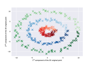
(a) 2D Input Data

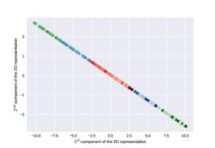
(b) AE Reconstruction

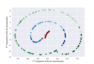
(c) KAE Reconstruction

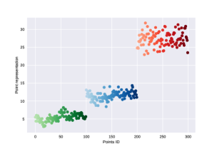
(d) 1D Representation (5 it.)

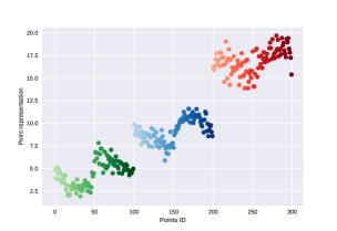
(e) 1D Representation (20 it.)

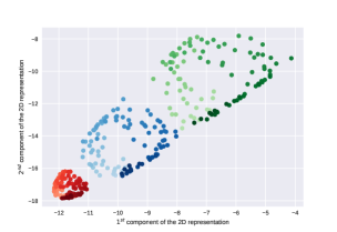
(f) 2D Re-Representation

Figure 3: KAE Performance on Noisy Concentric Circles

5.1 Behavior on a 2D problem

Let us first consider three noisy concentric circles such as in Figure 3(a). Although the main strength of KAEs is to perform autoencoding on complex data (Section 2.5), they can still be applied on real-valued points. Figures 3(b) and 3(c) show the reconstructions obtained after fitting respectively a 2-1-2 standard and kernel AE. Since the latent space is of dimension 1, the 2D reconstructions are manifolds of the same dimension, hence the curve aspect. What is interesting though is that the KAE learns a much more complex manifold than the standard AE. Due to its linear limitations (the nonlinear activation functions did not help much in this case), the standard AE returns a line, far from the original data, while the KAE outputs a more complex manifold, much closer to the initial data.

Apart from a good reconstruction, we are interested in finding representations with attractive properties. The 1D feature found by the previous KAE is interesting, as it is a discriminative one with respect to the original clusters: points from different circles are mapped around different values (Figure 3(d)). Interestingly, after a few iterations, some variability is introduced around these cluster values, so that all codes shall not be mapped back to the same point (Figure 3(e)).

Finally, a KAE with 1 hidden layer of size 2 gives the internal representation shown in Figure 3(f). This new 2D representation has a disentangling effect: the circle structure is kept so as to preserve the intra-cluster specificity, while the inter-cluster differentiation is ensured by the circles’ dissociation. These visual 2D examples give interesting insights on the good properties of the KAE representations: discrimination, disentanglement (see further experiments in Section C.1).

5.2 Representation Learning on Molecules

Table 1: NMSEs on Molecular Activity for Different Types of Cancer

	KRR	KPCA 10 + RF	KPCA 50 + RF	$\text{K}^{2}$AE 10 + RF	$\text{K}^{2}$AE 50 + RF
Cancer 01	0.02978	0.03279	0.03035	0.03097	0.02808
Cancer 02	0.03004	0.03194	0.02978	0.03099	0.02775
Cancer 03	0.02878	0.03155	0.02914	0.02989	0.02709
Cancer 04	0.03003	0.03274	0.03074	0.03218	0.02924
Cancer 05	0.02954	0.03185	0.02903	0.03065	0.02754
Cancer 06	0.02914	0.03258	0.03083	0.03134	0.02838
Cancer 07	0.03113	0.03468	0.03207	0.03257	0.03018
Cancer 08	0.02899	0.03162	0.02898	0.03065	0.02770
Cancer 09	0.02860	0.02992	0.02804	0.02872	0.02627
Cancer 10	0.02987	0.03291	0.03111	0.03170	0.02910

We now present an application of KAEs in the context of chemoinformatics. The motivation is triple. First, such complex data cannot be handled by standard AEs. Second, kernel methods being prominent in the field, data are often stored as Gram matrices, suiting perfectly our framework. Third, finding a compressed representation of a molecule is a problem of highest interest in Drug Discovery. We considered two different problems, one supervised, one unsupervised.

As for the supervised one, we exploited the dataset of Su et al., (2010) from the NCI-Cancer database: it consists in a Gram matrix comparing 2303 molecules by the mean of a Tanimoto kernel (a linear path kernel built using the presence or absence of sequences of atoms in the molecule), as well as the molecules activities in the presence of 59 types of cancer. The dataset containing no vectorial representations of the molecules (but only Gram matrices), only kernel methods were possible to benchmark. As a good representation is supposed to facilitate ulterior learning tasks, we assess the goodness of the representations through the regression scores obtained by Random Forests (RFs) from scikit-learn (Pedregosa et al.,, 2011) fed with it.

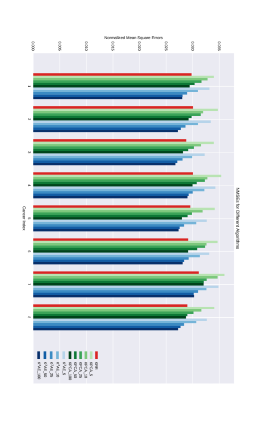
Figure 8: Performance of the Different Strategies on 8 Cancers

2-layer $\text{K}^{2}$AEs with respectively 5, 10, 25, 50 and 100 internal dimension were run, as well as Kernel Principal Component Analyses (KPCAs) with the same number of components. Finally, these representations were given as inputs to RFs. KRR was also added to the comparison. The Normalized Mean Squared Errors (NMSEs), averaged on 10 runs, for 5 strategies and on the first 10 cancers are stored in Table 1 (the complete results are available in Section C.2). A visualization with all strategies is also proposed in Figure 8. Clearly, methods combining a data representation step followed by a prediction one performs better. But the good performance of our approach should not be attributed to the use of RFs only, since the same strategy run with KPCA leads to worse results. Indeed, the $\text{K}^{2}$AE 50 + RF strategy outperforms all other procedures on all problems, managing to extract compact and useful feature vectors from the molecules.

Table 2: MSREs on Test Metabolites

Dimension	AE (sigmoid)	AE (relu)	KAE
5	99.81	96.62	76.38
10	87.36	84.02	65.76
25	72.31	68.77	51.63
50	63.00	58.29	40.72
100	55.43	48.63	36.27

The data for the unsupervised problem is taken from Brouard et al., 2016a . It is composed of two sets (a train set of size 5579, and a test set of size 1395), each one containing metabolites under the form of 4136-long binary vectors (called fingerprints), as well as a Gram matrix comparing them. 2-layer standard AEs from Keras (Chollet et al.,, 2015) with sigmoid and relu activation functions, and 2-layer KAEs with internal layer of size 5, 10, 25, 50 and 100, were trained. In absence of a supervised task, we measured the Mean Squared Reconstruction Errors (MSREs) induced on the test set, and stored them in Table 2. Again, the KAE approach shows a systematic improvement.

6 CONCLUSION

We introduce a new framework for AEs, based on vv-RKHSs and OVKs. The use of RKHS functions enables KAEs to handle data from possibly infinite dimensional Hilbert spaces, and then to extend the autoencoding scheme to any kind of data. A generalization bound and a strong connection to KPCA are established, while the underlying optimization problem is tackled by a Representer Theorem and the kernel trick. Beyond a detailed description, the behavior of the algorithm is carefully studied on simulated data, and yields relevant performances on graph data, that standard AEs are typically unable to handle. Further research may consider a semi-supervised approach, that would ideally tailor the representation according to the future targeted.

Acknowledgment

This work has been funded by the Industrial Chair Machine Learning for Big Data from Télécom ParisTech, Paris, France.

Appendix A TECHNICAL PROOFS

A.1 Proof of Theorem 1

Let $(\lambda_{1},\;\ldots,\;\lambda_{L})\in\mathbb{R}_{+}^{L}$ and $(f_{1}^{*},\;\ldots,\;f_{L}^{*})$ a solution to problem (6). Let $s_{l}=\|f_{l}^{*}\|_{\mathcal{H}_{l}}^{2}~{}\forall~{}l\in\llbracket L\rrbracket$. We shall prove that $(f_{1}^{*},\;\ldots,\;f_{L}^{*})$ is also a solution to problem (7) for this choice of $(s_{1},\ldots,s_{L})$. Consider $(f_{1},\;\ldots,\;f_{L})$ satisfying problem (7)’s constraints. $\forall~{}l\in\llbracket L\rrbracket,~{}\|f_{l}\|_{\mathcal{H}_{l}}^{2}\leq s_{l}=\|f_{l}^{*}\|_{\mathcal{H}_{l}}^{2}$. Hence, we have $\sum_{l=1}^{L}\lambda_{l}\|f_{l}\|_{\mathcal{H}_{l}}^{2}\leq\sum_{l=1}^{L}\lambda_{l}\|f_{l}^{*}\|_{\mathcal{H}_{l}}^{2}$. On the other hand, by definition of the $f_{l}^{*}$’s, it holds :

$$V(f_{1},\ldots,f_{L})+\sum_{l=1}^{L}\lambda_{l}\|f_{l}\|_{\mathcal{H}_{l}}^{2}~{}\geq~{}V(f_{1}^{*},\ldots,f_{L}^{*})+\sum_{l=1}^{L}\lambda_{l}\|f_{l}^{*}\|_{\mathcal{H}_{l}}^{2}.$$

Thus, we necessarily have: $V(f_{1},\ldots,f_{d})~{}\geq~{}V(f_{1}^{*},\ldots,f_{d}^{*})$.

A similar argument can be used for local solutions, details are left to the reader. ∎

Although this result may appear rather simple, we thought it was worth mentioning as our setting is particularly unfriendly: the objective function $V$ is not assumed to be convex, and the variables $f_{l}$ are infinite dimensional. As a consequence, in absence of additional assumptions the converse statement (that solutions to problem (7) are also solutions to problem (6) for a suitable choice of $\lambda_{l}$’s) is not guaranteed. The proof indeed rely on the existence of Lagrangian multipliers, which has been shown when the variables are finite dimensional (KKT conditions), or when the objective function is assumed to be convex (Bauschke et al.,, 2011), but is not ensured in our case.

A.2 Proof of Theorem 5

The technical proof is structured as follows.

A.2.1 Standard Rademacher Generalization Bound

Let loss $\ell$ denote the squared norm on $\mathcal{X}_{0}$: $\forall x\in\mathcal{X}_{0},\ell(x)=\|x\|_{\mathcal{X}_{0}}^{2}$. Notice that, on the set considered, the mapping $\ell$ is $2M$-Lipschitz, and: $\ell(x_{i}-h(x_{i}))-\ell(x_{i^{\prime}}-h(x_{i^{\prime}}))\leq 4M^{2}$. Hence, by applying McDiarmid’s inequality, together with standard arguments in the statistical learning literature (symmetrization/randomization tricks, see e.g. Theorem 3.1 in Mohri et al., (2012)), one may show that, for any $\delta\in(0,1)$, we have with probability at least $1-\delta$:

$$\frac{1}{2}\left(\epsilon(\hat{h}_{n})-\epsilon^{*}\right)\leq\sup_{h\in\mathcal{H}_{s,t}}|\epsilon(h)-\hat{\epsilon}_{n}(h)|\leq 2\widehat{\mathscr{R}}_{n}\Big{(}\big{(}\ell\circ(\text{id}-\mathcal{H}_{s,t})\big{)}(S)\Big{)}+12M^{2}\sqrt{\frac{\ln\frac{2}{\delta}}{2n}}.$$ (15)

The subsequent results shall provide tools to bound the quantity $\widehat{\mathscr{R}}_{n}\Big{(}\big{(}\ell\circ(\text{id}-\mathcal{H}_{s,t})\big{)}(S)\Big{)}$ properly.

A.2.2 Operations on the Rademacher Average

As a first go, we state a preliminary lemma that establishes a comparison between Rademacher and Gaussian averages.

Lemma 7.

We have: $\forall n\geq 1$,

$$\widehat{\mathscr{R}}_{n}(\mathcal{C}(S))\leq\sqrt{\frac{\pi}{2}}~{}\widehat{\mathscr{G}}_{n}(\mathcal{C}(S)).$$

Proof.

The proof is based on the fact that $\gamma_{i,k}$ and $\sigma_{i,k}\left|\gamma_{i,k}\right|$ have the same distribution, combined with Jensen’s inequality. See also Lemma 4.5 in Ledoux and Talagrand, (1991). ∎

Hence, the application of the lemma above yields:

$$\widehat{\mathscr{R}}_{n}\Big{(}\big{(}\ell\circ(\text{id}-\mathcal{H}_{s,t})\big{)}(S)\Big{)} \leq 2\sqrt{2}M~{}\widehat{\mathscr{R}}_{n}\Big{(}\big{(}\text{id}-\mathcal{H}_{s,t}\big{)}(S)\Big{)},$$ (16)

$$\leq 2\sqrt{2}M~{}\left[\widehat{\mathscr{R}}_{n}\Big{(}\{\text{id}\}(S)\Big{)}+\widehat{\mathscr{R}}_{n}\Big{(}\mathcal{H}_{s,t}(S)\Big{)}\right],$$ (17)

$$\leq 2\sqrt{2}M~{}\widehat{\mathscr{R}}_{n}\Big{(}\mathcal{H}_{s,t}(S)\Big{)},$$ (18)

$$\widehat{\mathscr{R}}_{n}\Big{(}\big{(}\ell\circ(\text{id}-\mathcal{H}_{s,t})\big{)}(S)\Big{)} \leq 2\sqrt{\pi}M~{}\widehat{\mathscr{G}}_{n}\Big{(}\mathcal{H}_{s,t}(S)\Big{)},$$ (19)

where (16) directly results from Corollary 4 in Maurer, (2016) (observing that, even if they do not take their values in $\ell_{2}(\mathbb{N})$ but in the separable Hilbert space $\mathcal{X}_{0}$, the functions $h(x)$ can replaced by the square-summable sequence $\left(\left\langle h(x),e_{k}\right\rangle\right)_{k\in\mathbb{N}}$) and (19) is a consequence of Lemma 7.

It now remains to bound $\widehat{\mathscr{G}}_{n}\Big{(}\mathcal{H}_{s,t}(S)\Big{)}$ using an extension of a result established in Maurer, (2014) and applying to classes of functions valued in $\mathbb{R}^{m}$ only, while functions in $\mathcal{H}_{s,t}$ are Hilbert-valued.

A.2.3 Extension of Maurer’s Chain Rule

The result stated below extends Theorem 2 in Maurer, (2014) to the Hilbert-valued situation.

Theorem 8.

Let $H$ be a Hilbert space, $X$ a $H$-valued Gaussian random vector, and $f:H\rightarrow\mathbb{R}$ a $L$-Lipschitz mapping. We have:

$$\forall t>0,\qquad\mathbb{P}\Big{(}\left|f(X)-\mathbb{E}f(X)\right|>t\Big{)}\leq\exp\left(-\frac{2t^{2}}{\pi^{2}L^{2}}\right).$$

Proof.

It is a direct extension of Corollary 2.3 in Pisier, (1986), which states the result for $H=\mathbb{R}^{N}$ only, observing that the proof given therein actually makes no use of the assumption of finite dimensionality of $H$, and thus remains valid in our case. Up to constants, it can also be viewed an extension of Theorem 4 in Maurer, (2014). ∎

We now introduce quantities involved in the rest of the analysis, see Definition 1 in Maurer, (2014).

Definition 9.

Let $Y\subset\mathbb{R}^{n}$, $H$ be a Hilbert space, $Z\subset H$, and $\gamma$ be a $H$-valued standard Gaussian variable/process. We set:

$$D(Y)=\sup_{y,y^{\prime}\in Y}\|y-y^{\prime}\|_{\mathbb{R}^{n}},$$

$$G(Z)=\sup_{z\in Z}\mathbb{E}_{\gamma}\left[\left\langle\gamma,z\right\rangle_{H}\right].$$

If $\mathcal{H}$ a class of functions from $Y$ to $H$, we set:

$$L(\mathcal{H},Y)=\sup_{h\in\mathcal{H}}~{}\sup_{y,y^{\prime}\in Y,~{}y\neq y^{\prime}}\frac{\|h(y)-h(y^{\prime})\|_{H}}{\|y-y^{\prime}\|_{\mathbb{R}^{n}}},$$

$$R(\mathcal{H},Y)=\sup_{y,y^{\prime}\in Y,~{}y\neq y^{\prime}}\mathbb{E}_{\bm{\gamma}}\left[\sup_{h\in\mathcal{H}}\frac{\left\langle\bm{\gamma},h(y)-h(y^{\prime})\right\rangle_{H}}{\|y-y^{\prime}\|_{\mathbb{R}^{n}}}\right].$$

The next result establishes useful relationships between the quantities introduced above.

Theorem 10.

Let $Y\subset\mathbb{R}^{n}$ be a finite set, $H$ a Hilbert space and $\mathcal{H}$ a finite class of functions $h:Y\rightarrow H$. Then, there are universal constants $C_{1}$ and $C_{2}$ such that, for any $y_{0}\in Y$:

$$G(\mathcal{H}(Y))\leq C_{1}L(\mathcal{H},Y)G(Y)+C_{2}R(\mathcal{H},Y)D(Y)+G(\mathcal{H}(y_{0})).$$

Proof.

This result is a direct extension of Theorem 2 in Maurer, (2014) for $H$-valued functions. The only part in the proof depending on the dimensionality of $H$ is Theorem 4 in the same paper, whose extension to any Hilbert space in Theorem 8 is proved in the present paper. Indeed, considering $X_{y}=(\sqrt{2}/\pi L(F,Y))\sup_{f\in F}\left\langle\gamma,f(y)\right\rangle$ (using the same notation as in Maurer, (2014) allows to finish the proof like in the finite dimensional case. ∎

Let $\mathcal{H}_{1,s}^{\prime}$ be the set of functions from $(\mathcal{X}_{0})^{n}$ to $\mathbb{R}^{np}$ that take as input $S=(x_{1},\ldots,x_{n})$ and return $(f(x_{1}),\ldots,f(x_{n}))$, $f\in\mathcal{H}_{1,s}$. Let $Y=\mathcal{H}_{1,s}^{\prime}(S)\subset\mathbb{R}^{np}$, and $H=(\mathcal{X}_{0})^{n}$, which is a Hilbert space. Let $\mathcal{H}=\mathcal{H}_{2,t}^{\prime}$ be the set of functions from $\mathbb{R}^{np}$ to $(\mathcal{X}_{0})^{n}$ that take as input $(y_{1},\ldots,y_{n})$ and return $(g(y_{1}),\ldots,g(y_{n}))$, $g\in\mathcal{H}_{2,t}$. Finally, let $y_{0}=(0_{\mathbb{R}^{p}},\ldots,0_{\mathbb{R}^{p}})$ (it actually belongs to $\mathcal{H}_{1,s}^{\prime}(S)$ since the null function is in $\mathcal{H}_{1,s}^{\prime}$). Theorem 10 entails that:

$$G\Big{(}\mathcal{H}_{2,t}^{\prime}\big{(}\mathcal{H}_{1,s}^{\prime}(S)\big{)}\Big{)}\leq C_{1}L\Big{(}\mathcal{H}_{2,t}^{\prime},\mathcal{H}_{1,s}^{\prime}(S)\Big{)}G\Big{(}\mathcal{H}_{1,s}^{\prime}(S)\Big{)}+C_{2}R\Big{(}\mathcal{H}_{2,t}^{\prime},\mathcal{H}_{1,s}^{\prime}(S)\Big{)}D\Big{(}\mathcal{H}_{1,s}^{\prime}(S)\Big{)}+G\Big{(}\mathcal{H}_{2,t}^{\prime}(0)\Big{)},$$ (20)

and

$$\widehat{\mathscr{G}}_{n}\Big{(}\mathcal{H}_{s,t}(S)\Big{)}\leq C_{1}L\Big{(}\mathcal{H}_{2,t}^{\prime},\mathcal{H}_{1,s}^{\prime}(S)\Big{)}\widehat{\mathscr{G}}_{n}\Big{(}\mathcal{H}_{1,s}(S)\Big{)}+\frac{C_{2}}{n}R\Big{(}\mathcal{H}_{2,t}^{\prime},\mathcal{H}_{1,s}^{\prime}(S)\Big{)}D\Big{(}\mathcal{H}_{1,s}^{\prime}(S)\Big{)}+\frac{1}{n}G\Big{(}\mathcal{H}_{2,t}^{\prime}(0)\Big{)}.$$ (21)

We now bound each term appearing on the right-hand side.

Bounding $L\Big{(}\mathcal{H}_{2,t}^{\prime},\mathcal{H}_{1,s}^{\prime}(S)\Big{)}$. Consider the following hypothesis, denoting by $\|.\|_{*}$ the operator norm of any bounded linear operator.

Assumption 11.

There exists a constant $L<+\infty$ such that: $\forall(y,y^{\prime})\in\mathbb{R}^{p}$,

$$\big{\|}\mathcal{K}_{2}(y,y)-2\mathcal{K}_{2}(y,y^{\prime})+\mathcal{K}_{2}(y^{\prime},y^{\prime})\big{\|}_{*}\leq L^{2}~{}\|y-y^{\prime}\|_{\mathbb{R}^{p}}^{2}.$$

This assumption is not too much compelling since it is enough for $\mathcal{K}_{2}$ to be the sum of $M$ decomposable kernels $k_{m}(\cdot,\cdot)A_{m}$ such that the scalar feature maps $\phi_{m}$ are $L_{m}$-Lipschitz (the feature map of the Gaussian kernel with bandwidth $1/(2\sigma^{2})$ has Lipschitz constant $1/\sigma$ for instance), and the $A_{m}$ operators have finite operator norms $\sigma_{m}$. Indeed, we would have then: $\forall z\in\mathcal{X}_{0}$,

$$\left\|\Big{(}\mathcal{K}_{2}(y,y)-2\mathcal{K}_{2}(y,y^{\prime})+\mathcal{K}_{2}(y^{\prime},y^{\prime})\Big{)}z\right\|_{\mathcal{X}_{0}} =\left\|\left(\sum_{m=1}^{M}\|\phi_{m}(y)-\phi_{m}(y^{\prime})\|^{2}A_{m}\right)z\right\|_{\mathcal{X}_{0}},$$

$$\leq\sum_{m=1}^{M}\|\phi_{m}(y)-\phi_{m}(y^{\prime})\|^{2}\sigma_{m}~{}\|z\|_{\mathcal{X}_{0}},$$

$$\left\|\Big{(}\mathcal{K}_{2}(y,y)-2\mathcal{K}_{2}(y,y^{\prime})+\mathcal{K}_{2}(y^{\prime},y^{\prime})\Big{)}z\right\|_{\mathcal{X}_{0}} \leq\left(\sum_{m=1}^{M}L_{m}^{2}\sigma_{m}\right)\|y-y^{\prime}\|_{\mathbb{R}^{p}}^{2}~{}\|z\|_{\mathcal{X}_{0}},$$

$$\left\|\mathcal{K}_{2}(y,y)-2\mathcal{K}_{2}(y,y^{\prime})+\mathcal{K}_{2}(y^{\prime},y^{\prime})\right\|_{*} \leq\left(\sum_{m=1}^{M}L_{m}^{2}\sigma_{m}\right)\|y-y^{\prime}\|_{\mathbb{R}^{p}}^{2}.$$

Let $\mathcal{K}_{2}$ satisfy 11, $g\in\mathcal{H}_{2,t}^{\prime}$ and $(\bm{y},\bm{y^{\prime}})\in\mathbb{R}^{np}$. We have

$$\left\|g(\bm{y})-g(\bm{y^{\prime}})\right\|_{(\mathcal{X}_{0})^{n}}^{2} =\sum_{i=1}^{n}\left\|g(y_{i})-g(y_{i}^{\prime})\right\|_{\mathcal{X}_{0}}^{2},$$ (22)

$$=\sum_{i=1}^{n}\left\langle g(y_{i})-g(y_{i}^{\prime}),g(y_{i})-g(y_{i}^{\prime})\right\rangle_{\mathcal{X}_{0}},$$ (23)

$$=\sum_{i=1}^{n}\left\langle{\mathcal{K}_{2}}_{y_{i}}(g(y_{i})-g(y_{i}^{\prime})),g\right\rangle_{\mathcal{H}_{2}}-\left\langle{\mathcal{K}_{2}}_{y_{i}^{\prime}}(g(y_{i})-g(y_{i}^{\prime})),g\right\rangle_{\mathcal{H}_{2}},$$ (24)

$$\leq\|g\|_{\mathcal{H}_{2}}\sum_{i=1}^{n}~{}\left\|{\mathcal{K}_{2}}_{y_{i}}(g(y_{i})-g(y_{i}^{\prime}))-{\mathcal{K}_{2}}_{y_{i}^{\prime}}(g(y_{i})-g(y_{i}^{\prime}))\right\|_{\mathcal{H}_{2}},$$ (25)

$$\leq t~{}\sum_{i=1}^{n}~{}\sqrt{\left\langle g(y_{i})-g(y_{i}^{\prime}),\big{(}\mathcal{K}_{2}(y_{i},y_{i})-2\mathcal{K}_{2}(y_{i},y_{i}^{\prime})+\mathcal{K}_{2}(y_{i}^{\prime},y_{i}^{\prime})\big{)}(g(y_{i})-g(y_{i}^{\prime}))\right\rangle_{\mathcal{X}_{0}}},$$ (26)

$$\leq Lt~{}\sum_{i=1}^{n}~{}\left\|g(y_{i})-g(y_{i}^{\prime})\right\|_{\mathcal{X}_{0}}\|y_{i}-y_{i}^{\prime}\|_{\mathbb{R}^{p}},$$ (27)

$$\left\|g(\bm{y})-g(\bm{y^{\prime}})\right\|_{(\mathcal{X}_{0})^{n}}^{2} \leq Lt~{}\left\|g(\bm{y})-g(\bm{y^{\prime}})\right\|_{(\mathcal{X}_{0})^{n}}\left\|\bm{y}-\bm{y^{\prime}}\right\|_{\mathbb{R}^{np}},$$ (28)

$$\left\|g(\bm{y})-g(\bm{y^{\prime}})\right\|_{(\mathcal{X}_{0})^{n}} \leq Lt~{}\left\|\bm{y}-\bm{y^{\prime}}\right\|_{\mathbb{R}^{np}},$$ (29)

where (24) results from the reproducing property in vv-RKHSs (see Eq. (2.1) in Micchelli and Pontil, (2005)), (25) follows from Cauchy-Schwarz inequality, (26) is again a consequence of the reproducing property (Eq. (2.3) in Micchelli and Pontil, (2005)), (27) can be deduced from 11 and (28) is a consequence of Cauchy-Schwarz inequality as well. Hence, we finally have:

$$L\Big{(}\mathcal{H}_{2,t}^{\prime},\mathcal{H}_{1,s}^{\prime}(S)\Big{)}\leq L\Big{(}\mathcal{H}_{2,t}^{\prime},\mathbb{R}^{np}\Big{)}\leq Lt.$$ (30)

Bounding $\widehat{\mathscr{G}}_{n}\Big{(}\mathcal{H}_{1,s}^{\prime}(S)\Big{)}$. Consider the assumption below.

Assumption 12.

There exists a constant $K<+\infty$ such that: $\forall x\in\mathcal{X}_{0}$,

$$\text{{Tr}}\Big{(}\mathcal{K}_{1}(x,x)\Big{)}\leq Kp.$$

This assumption is mild as well, since the sum of $M$ decomposable kernels $k_{m}(\cdot,\cdot)A_{m}$ such that the scalar kernels are bounded by $\kappa_{m}$ (as $X$ is supposed to be bounded, any continuous kernel is valid). Indeed, we have: $\forall x\in\mathcal{X}_{0}$,

$$\textbf{Tr}\Big{(}\mathcal{K}_{1}(x,x)\Big{)}=\sum_{m=1}^{M}k_{m}(x,x)~{}\textbf{Tr}(A_{m})\leq\left(\sum_{m=1}^{M}\kappa_{m}\|A_{m}\|_{\infty}\right)p.$$

Let the OVK $\mathcal{K}_{1}$ satisfy 12 and be such that $\mathcal{H}_{1}$ is separable. We then know that there exists $\Phi\in\mathcal{L}(\ell_{2}(\mathbb{N}),\mathbb{R}^{p})$ such that: $\forall(x,x^{\prime})\in\mathcal{X}_{0},~{}\mathcal{K}_{1}(x,x^{\prime})=\Phi(x)\Phi^{*}(x^{\prime})$ and $\forall f\in\mathcal{H}_{1},\exists u\in\ell_{2}(\mathbb{N})$ such that $f(\cdot)=\Phi(\cdot)u,~{}~{}\|f\|_{\mathcal{H}_{1}}=\|u\|_{\ell_{2}}$ (see Micchelli and Pontil, (2005)). We have:

$$n~{}\widehat{\mathscr{G}}_{n}\Big{(}\mathcal{H}_{1,s}^{\prime}(S)\Big{)} =\mathbb{E}_{\bm{\gamma}}\left[\sup_{f\in\mathcal{H}_{1,s}}\sum_{i=1}^{n}\left\langle\bm{\gamma}_{i},f(x_{i})\right\rangle_{\mathbb{R}^{p}}\right],$$ (31)

$$=\mathbb{E}_{\bm{\gamma}}\left[\sup_{\|u\|_{\ell_{2}}\leq s}\sum_{i=1}^{n}\sum_{k=1}^{p}\gamma_{i,k},\left\langle\Phi(x_{i})u,e_{k}\right\rangle_{\mathbb{R}^{p}}\right],$$ (32)

$$=\mathbb{E}_{\bm{\gamma}}\left[\sup_{\|u\|_{\ell_{2}}\leq s}\left\langle u,\sum_{i=1}^{n}\sum_{k=1}^{p}\gamma_{i,k}\Phi^{*}(x_{i})e_{k}\right\rangle_{\ell_{2}}\right],$$ (33)

$$\leq s~{}\mathbb{E}_{\bm{\gamma}}\left[\left\|\sum_{i=1}^{n}\sum_{k=1}^{p}\gamma_{i,k}\Phi^{*}(x_{i})e_{k}\right\|_{\ell_{2}}\right],$$ (34)

$$\leq s~{}\sqrt{\mathbb{E}_{\bm{\gamma}}\left[\left\|\sum_{i=1}^{n}\sum_{k=1}^{p}\gamma_{i,k}\Phi^{*}(x_{i})e_{k}\right\|_{\ell_{2}}^{2}\right]},$$ (35)

$$\leq s~{}\sqrt{\sum_{i=1}^{n}\sum_{k=1}^{p}\left\langle\mathcal{K}(x_{i},x_{i})e_{k},e_{k}\right\rangle_{\mathbb{R}^{p}}},$$ (36)

$$\leq s~{}\sqrt{\sum_{i=1}^{n}\textbf{Tr}\Big{(}\mathcal{K}_{1}(x_{i},x_{i})\Big{)}},$$ (37)

$$n~{}\widehat{\mathscr{G}}_{n}(\mathcal{H}_{1,s}^{\prime}(S)) \leq s\sqrt{nKp},$$ (38)

where (34) follows from Cauchy-Schwarz inequality, (35) from Jensen’s inequality, (36) results from the orthogonality of the Gaussian variables introduced and (38) from 12. Finally, we have:

$$\widehat{\mathscr{G}}_{n}\Big{(}\mathcal{H}_{1,s}^{\prime}(S)\Big{)}\leq s\sqrt{\frac{Kp}{n}}.$$ (39)

Bounding $R\Big{(}\mathcal{H}_{2,t}^{\prime},\mathcal{H}_{1,s}^{\prime}(S)\Big{)}$. Consider the following hypothesis.

Assumption 13.

There exists a constant $L<+\infty$ such that: $\forall(y,y^{\prime})\in\mathbb{R}^{p}$,

$$\text{{Tr}}\Big{(}\mathcal{K}_{2}(y,y)-2\mathcal{K}_{2}(y,y^{\prime})+\mathcal{K}_{2}(y^{\prime},y^{\prime})\Big{)}\leq L^{2}~{}\|y-y^{\prime}\|_{\mathbb{R}^{p}}^{2}.$$

Suppose that the OVK $\mathcal{K}_{2}$ is the sum of $M$ decomposable kernels $k_{m}(\cdot,\cdot)A_{m}$ such that the scalar feature maps $\phi_{m}$ are $L_{m}$-Lipschitz and the $A_{m}$ operators are trace class. Then, we have: $\forall(y,y^{\prime})\in\mathbb{R}^{p}$,

$$\textbf{Tr}\Big{(}\mathcal{K}_{2}(y,y)-2\mathcal{K}_{2}(y,y^{\prime})+\mathcal{K}_{2}(y^{\prime},y^{\prime})\Big{)}=\sum_{m=1}^{M}\|\phi_{m}(y)-\phi_{m}(y^{\prime})\|^{2}~{}\textbf{Tr}(A_{m})\leq\left(\sum_{m=1}^{M}L_{m}^{2}\textbf{Tr}(A_{m})\right)\|y-y^{\prime}\|_{\mathbb{R}^{p}}^{2}.$$

Note also that 13 is stronger than 11, since $\|A\|_{*}\leq\textbf{Tr}(A)$ for any trace class operator $A$.

Let the OVK $\mathcal{K}_{2}$ satisfy 13 and be such that $\mathcal{H}_{2}$ is separable. We then know that there exists $\Psi\in\mathcal{L}(\ell_{2}(\mathbb{N}),\mathcal{X}_{0})$ such that $\forall(y,y^{\prime})\in\mathbb{R}^{p},~{}\mathcal{K}_{2}(y,y^{\prime})=\Psi(y)\Psi^{*}(y^{\prime})$ and $\forall g\in\mathcal{H}_{2},\exists v\in\ell_{2}(\mathbb{N})$ such that $g(\cdot)=\Psi(\cdot)v,~{}~{}\|g\|_{\mathcal{H}_{2}}=\|v\|_{\ell_{2}}$. We have:

$$\mathbb{E}_{\bm{\gamma}}\left[\sup_{g\in\mathcal{H}_{2,t}}\left\langle\bm{\gamma}_{i},g(\bm{y}-g(\bm{y^{\prime}})\right\rangle_{\mathcal{X}_{0}^{n}}\right] =\mathbb{E}_{\bm{\gamma}}\left[\sup_{g\in\mathcal{H}_{2,t}}\sum_{i=1}^{n}\sum_{k=1}^{\infty}\gamma_{i,k}\left\langle(\Psi(y_{i})-\Psi(y^{\prime}_{i}))v,e_{k}\right\rangle_{\mathcal{X}_{0}}\right],$$ (40)

$$=\mathbb{E}_{\bm{\gamma}}\left[\sup_{g\in\mathcal{H}_{2,t}}\left\langle\sum_{i=1}^{n}\sum_{k=1}^{\infty}\gamma_{i,k}(\Psi^{*}(y_{i})-\Psi^{*}(y^{\prime}_{i}))e_{k},v\right\rangle_{\ell_{2}}\right],$$ (41)

$$\leq t~{}\sqrt{\mathbb{E}_{\bm{\gamma}}\left\|\sum_{i=1}^{n}\sum_{k=1}^{\infty}\gamma_{i,k}(\Psi^{*}(y_{i})-\Psi^{*}(y^{\prime}_{i}))e_{k}\right\|_{\ell_{2}}^{2}},$$ (42)

$$\leq t~{}\sqrt{\sum_{i=1}^{n}\textbf{Tr}\Big{(}\mathcal{K}_{2}(y_{i},y_{i})-2\mathcal{K}_{2}(y_{i},y^{\prime}_{i})+\mathcal{K}_{2}(y_{i}^{\prime},y_{i}^{\prime})\Big{)}},$$ (43)

$$\mathbb{E}_{\bm{\gamma}}\left[\sup_{g\in\mathcal{H}_{2,t}}\left\langle\bm{\gamma}_{i},g(\bm{y}-g(\bm{y^{\prime}})\right\rangle_{\mathcal{X}_{0}^{n}}\right] \leq tL~{}\|\bm{y}-\bm{y^{\prime}}\|_{\mathbb{R}^{np}},$$ (44)

where only 13 and arguments previously involved have been used. Finally, we get:

$$R\Big{(}\mathcal{H}_{2,t}^{\prime},\mathcal{H}_{1,s}^{\prime}(S)\Big{)}\leq R\Big{(}\mathcal{H}_{2,t}^{\prime},\mathbb{R}^{np}\Big{)}\leq tL.$$ (45)

Bounding $D\Big{(}\mathcal{H}_{1,s}^{\prime}(S)\Big{)}$. Consider the assumption below.

Assumption 14.

There exists $\kappa<+\infty$ such that: $\forall x\in S$,

$$\left\|\mathcal{K}_{1}(x,x)\right\|_{*}\leq\kappa^{2}.$$

This assumption is easily fulfilled, since $X$ is almost surely bounded. Indeed, any ov-kernel which is the (finite) sum of decomposable kernels with continuous scalar kernels fulfills it. Note also that it is a weaker assumption than 12, since one could choose $\kappa=\sqrt{Kp}$.

Let $\mathcal{K}_{1}$ satisfy 14 and $(\bm{y},\bm{y^{\prime}})\in\mathcal{H}_{1,s}^{\prime}(S)$. There exists $(f,f^{\prime})\in\mathcal{H}_{1,s}$ such that $\bm{y}=(f(x_{1}),\ldots,f(x_{n}))$ and $\bm{y^{\prime}}=(f^{\prime}(x_{1}),\ldots,f^{\prime}(x_{n}))$. We have:

$$\left\|\bm{y}-\bm{y^{\prime}}\right\|_{\mathbb{R}^{np}}^{2} =\sum_{i=1}^{n}\left\|f(x_{i})-f^{\prime}(x_{i})\right\|_{\mathbb{R}^{p}}^{2},$$ (46)

$$\leq\sum_{i=1}^{n}\left(\left\|f(x_{i})\right\|_{\mathbb{R}^{p}}+\left\|f^{\prime}(x_{i})\right\|_{\mathbb{R}^{p}}\right)^{2},$$ (47)

$$\leq\sum_{i=1}^{n}\left(\left\|f\right\|_{\mathcal{H}_{1}}\left\|\mathcal{K}_{1}(x_{i},x_{i})\right\|_{*}^{1/2}+\left\|f^{\prime}\right\|_{\mathcal{H}_{1}}\left\|\mathcal{K}_{1}(x_{i},x_{i})\right\|_{*}^{1/2}\right)^{2},$$ (48)

$$\left\|\bm{y}-\bm{y^{\prime}}\right\|_{\mathbb{R}^{np}}^{2} \leq 4\kappa^{2}s^{2}n,$$ (49)

where (48) follows from Eq. (f) of Proposition 2.1 in Micchelli and Pontil, (2005). Finally, we get:

$$D\Big{(}\mathcal{H}_{1,s}^{\prime},S\Big{)}\leq 2\kappa s\sqrt{n}.$$ (50)

Bounding $G\Big{(}\mathcal{H}_{2,t}^{\prime}(0)\Big{)}$. We introduce the following assumption.

Assumption 15.

$\mathcal{K}_{2}(0,0)$ is trace class.

Then, using the same arguments as for (37), we get:

$$n~{}G\Big{(}\mathcal{H}_{2,t}^{\prime}(0)\Big{)}\leq t\sqrt{n~{}\textbf{Tr}\Big{(}\mathcal{K}_{2}(0,0)\Big{)}},\text{\qquad or \qquad}G\Big{(}\mathcal{H}_{2,t}^{\prime}(0)\Big{)}\leq t\sqrt{\frac{\textbf{Tr}\big{(}\mathcal{K}_{2}(0,0)\big{)}}{n}}.$$ (51)

Rather than shifting the kernel $\widetilde{\mathcal{K}}_{2}(y,y^{\prime})=\mathcal{K}_{2}(y,y^{\prime})-\mathcal{K}_{2}(0,0)$, one could consider that 15 is always satisfied. In addition, we have $\textbf{Tr}\Big{(}\widetilde{\mathcal{K}}_{2}(0,0)\Big{)}=0$ and consequently $G\Big{(}\mathcal{H}_{2,t}^{\prime}(0)\Big{)}\leq 0$.

A.2.4 Final Argument

Now, combining inequalities (15), (19), (21), (30), (39), (45), (50) and defining $C_{0}\coloneqq 8\sqrt{\pi}(C_{1}+2C_{2})$, for any $\delta\in(0,1)$, we have with probability at least $1-\delta$:

$$\epsilon(\hat{h}_{n})-\epsilon^{*}\leq C_{0}LMst\sqrt{\frac{Kp}{n}}+24M^{2}\sqrt{\frac{\ln\frac{2}{\delta}}{2n}}.$$

∎

A.3 Proof of Theorem 6

Lemma 16.

See Theorem 3.1 in Micchelli and Pontil, (2005). Let $\mathcal{X}$ be a measurable space, $\mathcal{Y}$ a real Hilbert space with inner product $\left\langle\cdot,\cdot\right\rangle_{\mathcal{Y}}$, $\mathcal{K}:\mathcal{X}\times\mathcal{X}\rightarrow\mathcal{L}(\mathcal{Y})$ an operator-valued kernel, $\mathcal{H}\subset\mathcal{F}(\mathcal{X},\mathcal{Y})$ the corresponding vv-RKHS, with inner product $\langle\cdot,\cdot\rangle_{\mathcal{H}}$. We have the reproducing property : $\langle y,f(x)\rangle_{\mathcal{Y}}=\langle\mathcal{K}_{x}y,f\rangle_{\mathcal{H}}$, with the notation $\mathcal{K}_{x}y=\mathcal{K}(\cdot,x)y:\mathcal{X}\rightarrow\mathcal{Y}$. Suppose also that the linear functionals $L_{x_{i}}f=f(x_{i}),f\in\mathcal{H},i\in\llbracket n\rrbracket$ are linearly independent. Then the unique solution to the variational problem:

$$\min_{f\in\mathcal{H}}\Big{\{}\|f\|_{\mathcal{H}}^{2}:f(x_{i})=y_{i},~{}i\in\llbracket n\rrbracket\Big{\}},$$

is given by :

$$\hat{f}=\sum_{i=1}^{n}\mathcal{K}_{x_{i}}c_{i},$$

where $\{c_{i},~{}i\in\llbracket n\rrbracket\}\subset\mathcal{Y}^{n}$ is the unique solution of the linear system of equations :

$$\sum_{i=1}^{n}\mathcal{K}(x_{k},x_{i})c_{i}=y_{k},\qquad k\in\llbracket n\rrbracket.$$

Proof.

Let $f\in\mathcal{H}$ such that $f(x_{i})=y_{i}~{}~{}\forall~{}i\in\llbracket n\rrbracket$, and set $g=f-\hat{f}$. We have :

$$\|f\|_{\mathcal{H}}^{2}=\|\hat{f}\|_{\mathcal{H}}^{2}+\|g\|_{\mathcal{H}}^{2}+2\langle\hat{f},g\rangle_{\mathcal{H}}.$$

Observe also that :

$$\langle\hat{f},g\rangle_{\mathcal{H}}=\left\langle\sum_{i=1}^{n}\mathcal{K}_{x_{i}}c_{i},g\right\rangle_{\mathcal{H}}=\sum_{i=1}^{n}\langle\mathcal{K}_{x_{i}}c_{i},g\rangle_{\mathcal{H}}=\sum_{i=1}^{n}\langle c_{i},g(x_{i})\rangle_{\mathcal{Y}}=0.$$

Finally, we have :

$$\|f\|_{\mathcal{H}}^{2}=\|\hat{f}\|_{\mathcal{H}}^{2}+\|g\|_{\mathcal{H}}^{2}\geq\|\hat{f}\|_{\mathcal{H}}^{2}.$$

∎

Proof of Theorem 6.

We shall use the following shortcut notation:

$$\xi(f_{1}^{*},\ldots,f_{L_{0}}^{*},\mathcal{S})\coloneqq V\Big{(}(f_{L_{0}}\circ\ldots\circ f_{1})(x_{1}),\ldots,(f_{L_{0}}\circ\ldots\circ f_{1})(x_{n}),\left\|f_{1}\right\|_{\mathcal{H}_{1}},\ldots,\left\|f_{L_{0}}\right\|_{\mathcal{H}_{L_{0}}}\Big{)}.$$

Let $l_{0}\in\llbracket L_{0}\rrbracket$. Let $g_{l_{0}}\in\mathcal{H}_{l_{0}}$ such that :

$$g_{l_{0}}\left({x_{i}^{*}}^{(l_{0}-1)}\right)=f_{l_{0}}^{*}\left({x_{i}^{*}}^{(l_{0}-1)}\right),\qquad\forall~{}i\in\llbracket n\rrbracket.$$

By definition, we have :

$$\xi(f_{1}^{*},\ldots,f_{l_{0}}^{*},\ldots,f_{L_{0}}^{*},\mathcal{S})\leq\xi(f_{1}^{*},\ldots,g_{l_{0}},\ldots,f_{L_{0}}^{*},\mathcal{S}),$$

thus we necessarily have :

$$\|f_{l_{0}}^{*}\|_{\mathcal{H}_{l_{0}}}^{2}\leq\|g_{l_{0}}\|_{\mathcal{H}_{l_{0}}}^{2}.$$

Therefore $f_{l_{0}}^{*}$ is a solution to the problem :

$$\min_{f\in\mathcal{H}_{l_{0}}}\left\{~{}\|f\|_{\mathcal{H}_{l_{0}}}^{2}:f\left({x_{i}^{*}}^{(l_{0}-1)}\right)=f_{l_{0}}^{*}\left({x_{i}^{*}}^{(l_{0}-1)}\right),~{}i\in\llbracket n\rrbracket~{}\right\}.$$

From Lemma 16, there exists $\left(\varphi_{l_{0},1}^{*},\ldots,\varphi_{l_{0},n}^{*}\right)\in\mathcal{X}_{l_{0}}^{n}$, such that :

$$f_{l_{0}}^{*}(\cdot)=\sum_{i=1}^{n}\mathcal{K}_{l_{0}}\left(~{}\cdot~{},{x_{i}^{*}}^{(l_{0}-1)}\right)\varphi_{l_{0},i}^{*}.$$

∎

A.4 Non-convexity of the Problem

A.4.1 Functional Setting

We prove that problem (3) is not convex by showing that the objective function $(f,g)\mapsto\hat{\epsilon}_{n}(g\circ f)+\Omega(f,g)$ is not. We denote this application by $\mathcal{O}$ and suppose it is. If it were convex, one would have :

$$\mathcal{O}\left(\kappa(f,g)+(1-\kappa)(f^{\prime},g^{\prime})\right)~{}\leq~{}\kappa\mathcal{O}(f,g)+(1-\kappa)\mathcal{O}(f^{\prime},g^{\prime}),$$ (52)

for any $\kappa\in[0,1]$ and any functions $f,f^{\prime},g,g^{\prime}\in\mathcal{H}_{1}^{2}\times\mathcal{H}_{2}^{2}$. Now, consider the particular case where we want to encode a single point ($n=1$) from $\mathcal{X}_{0}=\mathbb{R}$ to $\mathcal{X}_{1}=\mathbb{R}$, using one single hidden layer ($L=2$). Let $x_{1}=1$, and assume that both kernels are linear : $\mathcal{K}_{1}(x,x^{\prime})=xx^{\prime}$, $\mathcal{K}_{2}(y,y^{\prime})=yy^{\prime}$. $f:x\mapsto\mathcal{K}_{1}(x,x_{1})\varphi=\varphi x$ and $f^{\prime}:x\mapsto\mathcal{K}_{1}(x,x_{1})\varphi^{\prime}=\varphi^{\prime}x$ are elements of $\mathcal{H}_{1}$ for any coefficients $\varphi,\varphi^{\prime}$. In the same way, $g:y\mapsto\mathcal{K}_{2}(y,f(x_{1}))\psi=\psi f(1)y$ and $g^{\prime}:y\mapsto\mathcal{K}_{2}(y,f^{\prime}(x_{1}))\psi^{\prime}=\psi^{\prime}f^{\prime}(1)y$ are elements of $\mathcal{H}_{2}$ for any $\psi,\psi^{\prime}\in\mathbb{R}^{2}$.

Therefore, $\mathcal{O}(f,g)$ depends only on $\varphi$ and $\psi$. Let $\mathcal{P}$ denote the application from $\mathbb{R}^{2}$ to $\mathbb{R}$ such that $\mathcal{O}(f,g)=\mathcal{P}(\varphi,\psi)$. Then, one has also $\mathcal{O}(f^{\prime},g^{\prime})=\mathcal{P}(\varphi^{\prime},\psi^{\prime})$. And finally, it holds :

$$\mathcal{O}\left(\kappa(f,g)+(1-\kappa)(f^{\prime},g^{\prime})\right) =\mathcal{O}\left(\kappa f+(1-\kappa)f^{\prime},\kappa g+(1-\kappa)g^{\prime})\right),$$

$$=\mathcal{P}\left(\kappa\varphi+(1-\kappa)\varphi^{\prime},\kappa\psi+(1-\kappa)\psi^{\prime})\right),$$

$$\mathcal{O}\left(\kappa(f,g)+(1-\kappa)(f^{\prime},g^{\prime})\right) =\mathcal{P}\left(\kappa(\varphi,\psi)+(1-\kappa)(\varphi^{\prime},\psi^{\prime})\right).$$

So if (52) were true, in particular it would be true for the specific $f,f^{\prime},g,g^{\prime}$ functions we just defined. Hence, the following would hold for any $\varphi,\varphi^{\prime},\psi,\psi^{\prime}\in\mathbb{R}^{4}$ :

$$\mathcal{P}\left(\kappa(\varphi,\psi)+(1-\kappa)(\varphi^{\prime},\psi^{\prime})\right)~{}\leq~{}\kappa\mathcal{P}(\varphi,\psi)+(1-\kappa)\mathcal{P}(\varphi^{\prime},\psi^{\prime}).$$

This is exactly the convexity of $\mathcal{P}$ in $(\varphi,\psi)$. So the convexity of the objective function in the functional setting (problem (3)) implies the convexity of the objective function in the parametric setting (obtained after application of Theorem 6). In the following section we show that the latest does not even hold, which allows to conclude that neither problem is convex.

A.4.2 Parametric Setting

As a reminder, we have :

$$f(x)=\mathcal{K}_{1}(x,x_{1})\varphi=\varphi x,\qquad f(1)=\varphi,$$

$$g(y)=\mathcal{K}_{2}(y,f(x_{1}))\psi=\varphi\psi y, g(f(1))=\varphi^{2}\psi.$$

Our problem reads :

$$\min_{\varphi\in\mathbb{R},~{}\psi\in\mathbb{R}}~{}~{}\mathcal{P}(\varphi,\psi)\overset{def}{=}\left(1-\varphi^{2}\psi\right)^{2}+\lambda\varphi^{2}+\mu\psi^{2},$$

or equivalently :

$$\min_{\varphi\in\mathbb{R},~{}\psi\in\mathbb{R}}~{}~{}1+\lambda\varphi^{2}+\mu\psi^{2}-2\varphi^{2}\psi+\varphi^{4}\psi^{2}.$$

Let us find the critical points and analyze them. We have :

$$\frac{\partial\mathcal{P}}{\partial\varphi}(\varphi,\psi) = 2\lambda\varphi-4\varphi\psi+4\varphi^{3}\psi^{2},$$

$$\frac{\partial\mathcal{P}}{\partial^{2}\varphi}(\varphi,\psi) = 2\lambda-4\psi+12\varphi^{2}\psi^{2},$$

$$\frac{\partial\mathcal{P}}{\partial\psi}(\varphi,\psi) = 2\mu\psi-2\varphi^{2}+2\varphi^{4}\psi,$$

$$\frac{\partial\mathcal{P}}{\partial^{2}\psi}(\varphi,\psi) = 2\mu+2\varphi^{4},$$

$$\frac{\partial\mathcal{P}}{\partial\varphi\partial\psi}(\varphi,\psi) = -4\varphi+8\varphi^{3}\psi.$$

The two following equivalence relationships hold true:

$$\frac{\partial\mathcal{P}}{\partial\varphi}(\varphi^{*},\psi^{*}) =\left(2\lambda-4\psi^{*}+4{\varphi^{*}}^{2}{\psi^{*}}^{2}\right)\varphi^{*}=0 \Leftrightarrow\qquad\varphi^{*}=0\text{~{}~{}or~{}~{}}{\varphi^{*}}^{2}=\frac{2\psi^{*}-\lambda}{2{\psi^{*}}^{2}},\qquad\qquad$$

$$\frac{\partial\mathcal{P}}{\partial\psi}(\varphi^{*},\psi^{*}) =2\mu\psi^{*}-2{\varphi^{*}}^{2}+2{\varphi^{*}}^{4}\psi^{*}=0 \Leftrightarrow\qquad\psi^{*}=\frac{{\varphi^{*}}^{2}}{{\varphi^{*}}^{4}+\mu}.$$

Obviously, the point $(\varphi^{*},\psi^{*})=(0,0)$ is always critical. Notice that :

$$\textbf{Hess}_{(0,0)}\mathcal{P}=\left(\begin{matrix}2\lambda&0\\ 0&2\mu\end{matrix}\right)\succ 0.$$

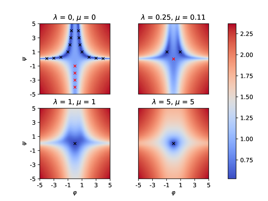
Figure 4: Heatmaps of $\mathcal{P}$ for different values of $\lambda$ and $\mu$

Thus $(0,0)$ is a local minimum and $\mathcal{P}(0,0)=1$. To prove that it is not a global minimizer, it is enough to find a couple $(\varphi,\psi)$ such that $\mathcal{P}(\varphi,\psi)<1$. For example $\mathcal{P}(1,1)=\lambda+\mu$. As soon as $\lambda+\mu<1$, the objective $\mathcal{P}$ is not invex, and a fortiori non-convex.

Figure 4 shows the heatmaps of $\mathcal{P}$ with respect to $\varphi$ and $\psi$ for different regularization settings. Note that in the non-regularized setting ($\lambda=\mu=0$), every point $(0,\psi)$ with $\psi<0$ is a local minimizer but not a global one. They are represented by red crosses. On the other hand, we have also an infinite number of global minima, namely every couple satisfying $\varphi^{2}\psi=1$. See the black crosses on the top left figure. When the regularization parameters remain small enough, $(0,0)$ is a local minimizer but not a global one (top right figure). Finally, the higher the regularization, the smoother the objective, even if convexity can never be verified (bottom figures).

Appendix B Gradient Derivation Details

B.1 Detail of Equation (10)

$$\|f_{l}\|_{\mathcal{H}_{l}}^{2} =\left\langle f_{l},f_{l}\right\rangle_{\mathcal{H}_{l}},$$

$$=\left\langle\sum_{i=1}^{n}\mathcal{K}_{l}\left(~{}.~{},{x_{i}}^{(l-1)}\right)\varphi_{l,i}~{},~{}\sum_{i^{\prime}=1}^{n}\mathcal{K}_{l}\left(~{}.~{},{x_{i^{\prime}}}^{(l-1)}\right)\varphi_{l,i^{\prime}}\right\rangle_{\mathcal{H}_{l}},$$

$$=\sum_{i,i^{\prime}=1}^{n}\left\langle\mathcal{K}_{l}\left(~{}.~{},{x_{i}}^{(l-1)}\right)\varphi_{l,i}~{},~{}\mathcal{K}_{l}\left(~{}.~{},{x_{i^{\prime}}}^{(l-1)}\right)\varphi_{l,i^{\prime}}\right\rangle_{\mathcal{H}_{l}},$$

$$=\sum_{i,i^{\prime}=1}^{n}\left\langle\varphi_{l,i}~{},~{}\mathcal{K}_{l}\left({x_{i}}^{(l-1)},{x_{i^{\prime}}}^{(l-1)}\right)\varphi_{l,i^{\prime}}\right\rangle_{\mathcal{X}_{l}},$$

$$\|f_{l}\|_{\mathcal{H}_{l}}^{2} =\sum_{i,i^{\prime}=1}^{n}k_{l}\left({x_{i}}^{(l-1)},{x_{i^{\prime}}}^{(l-1)}\right)\left\langle\varphi_{l,i}~{},~{}A_{l}~{}\varphi_{l,i^{\prime}}\right\rangle_{\mathcal{X}_{l}}.$$

∎

B.2 Detail of Equation (12)

$$\Big{(}\nabla_{\varphi_{l_{0},i_{0}}}~{}\|f_{l}\|_{\mathcal{H}_{l}}^{2}\Big{)}^{\top} =\sum_{i,i^{\prime}=1}^{n}[N_{l}]_{i,i^{\prime}}\left(\nabla_{\varphi_{l_{0},i_{0}}}~{}k_{l}\left({x_{i}}^{(l-1)},{x_{i^{\prime}}}^{(l-1)}\right)\right)^{\top},$$

$$=\sum_{i,i^{\prime}=1}^{n}[N_{l}]_{i,i^{\prime}}~{}\bigg{[}~{}\left(\nabla^{(1)}k_{l}\left({x_{i}}^{(l-1)},{x_{i^{\prime}}}^{(l-1)}\right)\right)^{\top}\textbf{Jac}_{{x_{i}}^{(l-1)}}(\varphi_{l_{0},i_{0}})$$

$$\phantom{=\sum_{i,i^{\prime}=1}^{n}[N_{l}]_{i,i^{\prime}}~{}\bigg{[}~{}}+\left(\nabla^{(2)}k_{l}\left({x_{i}}^{(l-1)},{x_{i^{\prime}}}^{(l-1)}\right)\right)^{\top}\textbf{Jac}_{{x_{i^{\prime}}}^{(l-1)}}(\varphi_{l_{0},i_{0}})~{}\bigg{]},$$

$$=\sum_{i,i^{\prime}=1}^{n}[N_{l}]_{i,i^{\prime}}\left(\nabla^{(1)}k_{l}\left({x_{i}}^{(l-1)},{x_{i^{\prime}}}^{(l-1)}\right)\right)^{\top}\textbf{Jac}_{{x_{i}}^{(l-1)}}(\varphi_{l_{0},i_{0}})$$

$$\phantom{=}+\sum_{i^{\prime},i=1}^{n}[N_{l}]_{i^{\prime},i}\left(\nabla^{(1)}k_{l}\left({x_{i^{\prime}}}^{(l-1)},{x_{i}}^{(l-1)}\right)\right)^{\top}\textbf{Jac}_{{x_{i^{\prime}}}^{(l-1)}}(\varphi_{l_{0},i_{0}}),$$

$$\Big{(}\nabla_{\varphi_{l_{0},i_{0}}}~{}\|f_{l}\|_{\mathcal{H}_{l}}^{2}\Big{)}^{\top} =2\sum_{i,i^{\prime}=1}^{n}[N_{l}]_{i,i^{\prime}}\left(\nabla^{(1)}k_{l}\left({x_{i}}^{(l-1)},{x_{i^{\prime}}}^{(l-1)}\right)\right)^{\top}\textbf{Jac}_{{x_{i}}^{(l-1)}}(\varphi_{l_{0},i_{0}}),$$

where $\nabla^{(1)}k_{l}\left(x,x^{\prime}\right)$ (respectively $\nabla^{(2)}k_{l}\left(x,x^{\prime}\right)$) denotes the gradient of $k_{l}(\cdot,\cdot)$ with respect to the $1^{st}$ (respectively $2^{nd}$) coordinate evaluated in $\left(x,x^{\prime}\right)$. ∎

B.3 Detail of Jacobians Computation

All previously written gradients involve Jacobian matrices. Their computation is to be detailed in this subsection. First note that $\textbf{Jac}_{{x_{i}}^{(l)}}(\varphi_{l_{0},i_{0}})$ only makes sense if $l_{0}\leq l$. Indeed, ${x_{i}}^{(l)}$ is completely independent from $\varphi_{l_{0},i_{0}}$ otherwise. Let us first detail ${x_{i}}^{(l)}$ and use the linearity of the Jacobian operator :

$$\textbf{Jac}_{{x_{i}}^{(l)}}(\varphi_{l_{0},i_{0}})=\sum_{i^{\prime}=1}^{n}\textbf{Jac}_{k_{l}\left({x_{i}}^{(l-1)},{x_{i^{\prime}}}^{(l-1)}\right)A_{l}~{}\varphi_{l,i^{\prime}}}(\varphi_{l_{0},i_{0}}).$$

Just as in the norm gradient case (see Section 4.2), there are two different outputs depending on whether $l=l_{0}$ (this gives an initialization), or $l>l_{0}$ (this leads to a recurrence formula).

Own Jacobian $(l=l_{0})$ :

$$\textbf{Jac}_{{x_{i}}^{(l)}}(\varphi_{l,i_{0}}) =\sum_{i^{\prime}=1}^{n}\textbf{Jac}_{k_{l}\left({x_{i}}^{(l-1)},{x_{i^{\prime}}}^{(l-1)}\right)A_{l}~{}\varphi_{l,i^{\prime}}}(\varphi_{l,i_{0}}),$$

$$=\sum_{i^{\prime}=1}^{n}k_{l}\left({x_{i}}^{(l-1)},{x_{i^{\prime}}}^{(l-1)}\right)\textbf{Jac}_{A_{l}~{}\varphi_{l,i^{\prime}}}(\varphi_{l,i_{0}}),$$

$$\textbf{Jac}_{{x_{i}}^{(l)}}(\varphi_{l,i_{0}}) =[K_{l}]_{i,i_{0}}~{}A_{l}.$$

Higher Jacobian $(l>l_{0})$ :

$$\textbf{Jac}_{{x_{i}}^{(l)}}(\varphi_{l_{0},i_{0}}) =\sum_{i^{\prime}=1}^{n}\textbf{Jac}_{k_{l}\left({x_{i}}^{(l-1)},{x_{i^{\prime}}}^{(l-1)}\right)A_{l}~{}\varphi_{l,i^{\prime}}}(\varphi_{l_{0},i_{0}}),$$

$$=\sum_{i^{\prime}=1}^{n}A_{l}~{}\varphi_{l,i^{\prime}}\left(\nabla_{\varphi_{l_{0},i_{0}}}~{}k_{l}\left({x_{i}}^{(l-1)},{x_{i^{\prime}}}^{(l-1)}\right)\right)^{\top},$$

$$=A_{l}\sum_{i^{\prime}=1}^{n}\varphi_{l,i^{\prime}}\bigg{[}~{}\left(\nabla^{(1)}k_{l}\left({x_{i}}^{(l-1)},{x_{i^{\prime}}}^{(l-1)}\right)\right)^{\top}\textbf{Jac}_{{x_{i}}^{(l-1)}}(\varphi_{l_{0},i_{0}})$$

$$\phantom{=A_{l}\sum_{i^{\prime}=1}^{n}\varphi_{l,i^{\prime}}\bigg{[}~{}}+\left(\nabla^{(1)}k_{l}\left({x_{i^{\prime}}}^{(l-1)},{x_{i}}^{(l-1)}\right)\right)^{\top}\textbf{Jac}_{{x_{i^{\prime}}}^{(l-1)}}(\varphi_{l_{0},i_{0}})~{}\bigg{]},$$

$$=~{}~{}A_{l}\left[\sum_{i^{\prime}=1}^{n}\varphi_{l,i^{\prime}}\left(\nabla^{(1)}k_{l}\left({x_{i}}^{(l-1)},{x_{i^{\prime}}}^{(l-1)}\right)\right)^{\top}\right]\textbf{Jac}_{{x_{i}}^{(l-1)}}(\varphi_{l_{0},i_{0}})$$

$$~{}~{}+A_{l}\left[\sum_{i^{\prime}=1}^{n}\varphi_{l,i^{\prime}}\left(\nabla^{(1)}k_{l}\left({x_{i^{\prime}}}^{(l-1)},{x_{i}}^{(l-1)}\right)\right)^{\top}\textbf{Jac}_{{x_{i^{\prime}}}^{(l-1)}}(\varphi_{l_{0},i_{0}})\right],$$

$$\textbf{Jac}_{{x_{i}}^{(l)}}(\varphi_{l_{0},i_{0}}) =A_{l}\Bigg{[}\Phi_{l}^{\top}\Delta_{l}\left({x_{i}}^{(l-1)}\right)\textbf{Jac}_{{x_{i}}^{(l-1)}}(\varphi_{l_{0},i_{0}})$$

$$~{}~{}~{}~{}~{}~{}~{}~{}~{}~{}~{}+\sum_{i^{\prime}=1}^{n}\varphi_{l,i^{\prime}}\left(\nabla^{(1)}k_{l}\left({x_{i^{\prime}}}^{(l-1)},{x_{i}}^{(l-1)}\right)\right)^{\top}\textbf{Jac}_{{x_{i^{\prime}}}^{(l-1)}}(\varphi_{l_{0},i_{0}})\Bigg{]},$$

with $\Delta_{l}(x)\coloneqq\left(\left(\nabla^{(1)}k_{l}\left(x,{x_{1}}^{(l-1)}\right)\right)^{\top},\ldots,\left(\nabla^{(1)}k_{l}\left(x,{x_{n}}^{(l-1)}\right)\right)^{\top}\right)^{\top}$ the $n\times d_{l-1}$ matrix storing the $\nabla^{(1)}k_{l}\left(x,{x_{i}}^{(l-1)}\right)$ in rows. These matrices are computed on Section B.4 (especially for $x={x_{i}}^{(l-1)})$. Assuming these quantities are known, we have an expression of $\textbf{Jac}_{{x_{i}}^{(l)}}(\varphi_{l_{0},i_{0}})$ that only depends on the $\textbf{Jac}_{{x_{i^{\prime}}}^{(l-1)}}(\varphi_{l_{0},i_{0}})$. Thus we can unroll the recurrence until $l=l_{0}$ and, using the previous subsection, compute $\textbf{Jac}_{{x_{i}}^{(l)}}(\varphi_{l_{0},i_{0}})$ for every couple $(l,l_{0})$ such that $l>l_{0}$.

An interesting remark can be made on the two-terms structure of the Jacobians. Indeed, the first term corresponds to the chain rule on ${x_{i}}^{(l)}=f_{l}\left({x_{i}}^{(l-1)}\right)$ assuming that $f_{l}$ is constant : $\frac{\partial f_{l}\left({x_{i}}^{(l-1)}\right)}{\partial\varphi_{l_{0},i_{0}}}=\frac{\partial f_{l}\left({x_{i}}^{(l-1)}\right)}{\partial{x_{i}}^{(l-1)}}\cdot\frac{\partial{x_{i}}^{(l-1)}}{\partial\varphi_{l_{0},i_{0}}}$ (notation abuse on $\partial$ in order to preserve understandability). On the contrary, the second term corresponds to a chain rule assuming that ${x_{i}}^{(l-1)}$ does not vary with $\varphi_{l_{0},i_{0}}$, but that $f_{l}$ does, through the influence of $\varphi_{l_{0},i_{0}}$ on the supports of $f_{l}$, namely the ${x_{i^{\prime}}}^{(l-1)}$.

B.4 Detail of the $\Delta_{l}$ Matrices Computation

In this section we derive the quantities $\nabla^{(1)}k_{l}\left({x_{i}}^{(l-1)},{x_{i^{\prime}}}^{(l-1)}\right)$ and more specifically the matrices $\Delta_{l}\left({x_{i}}^{(l-1)}\right)$ for $l\in\llbracket L\rrbracket$ and $i\in\llbracket n\rrbracket$. Note that all previously computed quantities are independent from the kernel chosen. Actually, the $\Delta_{l}\left({x_{i}}^{(l-1)}\right)$ matrices encapsulate all the kernel specificity of the algorithm. Thus, tailoring a new algorithm by changing the kernels only requires computing the new $\Delta_{l}$ matrices. This flexibility is a key asset of our approach, and more generally a crucial characteristic of kernel methods. In the following, we describe the $\Delta_{l}$ derivation for two popular kernels : the Gaussian and the polynomial ones.

Gaussian kernel :

$$\nabla^{(1)}k_{l}(x,x^{\prime})=\nabla_{x}\Big{(}\exp\left(-\gamma_{l}\|x-x^{\prime}\|_{\mathcal{X}_{l-1}}^{2}\right)\Big{)}=-2\gamma_{l}~{}e^{-\gamma_{l}\|x-x^{\prime}\|_{\mathcal{X}_{l-1}}^{2}}~{}(x-x^{\prime}).$$

$$\Delta_{l}\left({x_{i}}^{(l-1)}\right) =\bigg{[}\left(\nabla^{(1)}k_{l}\left({x_{i}}^{(l-1)},{x_{1}}^{(l-1)}\right)\right)^{\top},\ldots,\left(\nabla^{(1)}k_{l}\left({x_{i}}^{(l-1)},{x_{n}}^{(l-1)}\right)\right)^{\top}\bigg{]}^{\top},$$

$$=-2\gamma_{l}\bigg{[}e^{-\gamma_{l}\left\|{x_{i}}^{(l-1)}-{x_{1}}^{(l-1)}\right\|_{\mathcal{X}_{l-1}}^{2}}\left({x_{i}}^{(l-1)}-{x_{1}}^{(l-1)}\right)^{\top},\ldots$$

$$\phantom{=-2\gamma_{l}\bigg{[}}\ldots,e^{-\gamma_{l}\left\|{x_{i}}^{(l-1)}-{x_{n}}^{(l-1)}\right\|_{\mathcal{X}_{l-1}}^{2}}\left({x_{i}}^{(l-1)}-{x_{n}}^{(l-1)}\right)^{\top}\bigg{]}^{\top},$$

$$\Delta_{l}\left({x_{i}}^{(l-1)}\right) =-2\gamma_{l}~{}\tilde{K}_{l,i}\circ\left(\tilde{X}_{i}^{(l-1)}-X^{(l-1)}\right),$$

where :

• $X^{(l-1)}\coloneqq\left(\left({x_{1}}^{(l-1)}\right)^{\top},\ldots,\left({x_{n}}^{(l-1)}\right)^{\top}\right)^{\top}\in\mathbb{R}^{n\times d_{l-1}}$ stores the level $l-1$ representations of the $x_{i}$’s in rows

• $\tilde{X}_{i}^{(l-1)}\coloneqq\left(\left({x_{i}}^{(l-1)}\right)^{\top},\ldots,\left({x_{i}}^{(l-1)}\right)^{\top}\right)^{\top}\in\mathbb{R}^{n\times d_{l-1}}$ stores the level $l-1$ representation of $x_{i}$ $n$ times in rows

• $\tilde{K}_{l,i}\in\mathbb{R}^{n\times n}$ is the $k_{l}$ Gram matrix between $X^{(l-1)}$ and $\tilde{X}_{i}^{(l-1)}$ (i.e. $[\tilde{K}_{l,i}]_{s,t}=k_{l}\left({x_{i}}^{(l-1)},{x_{t}}^{(l-1)}\right)$)

• $\circ$ denotes the Hadamard (termwise) product for two matrices of the same shape

In practice, it is important to note that computing the $\Delta_{l}$ matrices with the Gaussian kernel needs not new calculations, but only uses already computed quantities : the level $l-1$ representations and their Gram matrix.

Polynomial kernel :

$$\nabla^{(1)}k_{l}(x,x^{\prime})=\nabla_{x}~{}\Big{(}\left(a\left\langle x,x^{\prime}\right\rangle+b\right)^{c}\Big{)}=ca\Big{(}\left(a\left\langle x,x^{\prime}\right\rangle+b\right)^{c-1}\Big{)}x^{\prime}.$$

$$\Delta_{l}\left({x_{i}}^{(l-1)}\right) =\bigg{[}\left(\nabla^{(1)}k_{l}\left({x_{i}}^{(l-1)},{x_{1}}^{(l-1)}\right)\right)^{\top},...~{},\left(\nabla^{(1)}k_{l}\left({x_{i}}^{(l-1)},{x_{n}}^{(l-1)}\right)\right)^{\top}\bigg{]}^{\top},$$

$$=ca\bigg{[}\left(a\left\langle{x_{i}}^{(l-1)},{x_{1}}^{(l-1)}\right\rangle+b\right)^{c-1}\left({x_{1}}^{(l-1)}\right)^{\top},\ldots$$

$$\qquad\quad\ldots,\left(a\left\langle{x_{i}}^{(l-1)},{x_{n}}^{(l-1)}\right\rangle+b\right)^{c-1}\left({x_{n}}^{(l-1)}\right)^{\top}\bigg{]}^{\top},$$

$$\Delta_{l}\left({x_{i}}^{(l-1)}\right) =ca~{}\left(\tilde{K}_{l,i}\right)^{\frac{c-1}{c}}\circ X^{(l-1)},$$

where we keep the notations introduced in the Gaussian kernel example for $X^{(l-1)}$, $\tilde{K}_{l,i}$ and $\circ$. Note that the exponent on $\tilde{K}_{l,i}$ must be understood as a termwise power, and not a matrix multiplication power.

In practice, it is important to note that computing the $\Delta_{l}$ matrices with the polynomial kernel only requires a slight and cheap new calculation : putting the - already computed - Gram matrix at layer $l-1$ to the termwise power $(c-1)/c$.

B.5 Detail of $N_{L}$ Computation

$$\left\langle x_{j},x_{j^{\prime}}\right\rangle_{\mathcal{X}_{0}} =\Bigg{\langle}\sum_{i=1}^{n}\left(\mathcal{K}_{L}\left(x_{j}^{(L-1)},x_{i}^{(L-1)}\right)+n\lambda_{L}\delta_{ij}\right)\varphi_{L,i}~{},$$

$$\quad\quad\sum_{i^{\prime}=1}^{n}\left(\mathcal{K}_{L}\left(x_{j^{\prime}}^{(L-1)},x_{i^{\prime}}^{(L-1)}\right)+n\lambda_{L}\delta_{i^{\prime}j^{\prime}}\right)\varphi_{L,i^{\prime}}\Bigg{\rangle}_{\mathcal{X}_{0}},$$

$$=\sum_{i,i^{\prime}=1}^{n}\Bigg{\langle}\left(k_{L}\left(x_{j}^{(L-1)},x_{i}^{(L-1)}\right)+n\lambda_{L}\delta_{ij}\right)\varphi_{L,i}~{},$$

$$\qquad\qquad~{}~{}\left(k_{L}\left(x_{j^{\prime}}^{(L-1)},x_{i^{\prime}}^{(L-1)}\right)+n\lambda_{L}\delta_{i^{\prime}j^{\prime}}\right)\varphi_{L,i^{\prime}}\Bigg{\rangle}_{\mathcal{X}_{0}},$$

$$\left\langle x_{j},x_{j^{\prime}}\right\rangle_{\mathcal{X}_{0}} =\sum_{i,i^{\prime}=1}^{n}\left(k_{L}\left(x_{j}^{(L-1)},x_{i}^{(L-1)}\right)+n\lambda_{L}\delta_{ij}\right)$$

$$\qquad\quad~{}~{}\left(k_{L}\left(x_{j^{\prime}}^{(L-1)},x_{i^{\prime}}^{(L-1)}\right)+n\lambda_{L}\delta_{i^{\prime}j^{\prime}}\right)\left\langle\varphi_{L,i},\varphi_{L,i^{\prime}}\right\rangle_{\mathcal{X}_{0}}.$$ (53)

As a reminder, $N_{L}$ denotes the matrix such that $[N_{L}]_{i,i^{\prime}}=\left\langle\varphi_{L,i},\varphi_{L,i^{\prime}}\right\rangle_{\mathcal{X}_{0}}$. Let $K_{in}$ denote the input Gram matrix such that $[K_{in}]_{j,j^{\prime}}=\left\langle x_{j},x_{j^{\prime}}\right\rangle_{\mathcal{X}_{0}}$. Finally, following notations of Section 4.2 for $K_{L}$, and denoting $I_{n}$ the identity matrix on $\mathbb{R}^{n}$, equation (B.5) may be rewritten as:

$$[K_{in}]_{j,j^{\prime}}=\sum_{i,i^{\prime}=1}^{n}[K_{L}+n\lambda_{L}I_{n}]_{j,i}[N_{L}]_{i,i^{\prime}}[K_{L}+n\lambda_{L}I_{n}]_{i^{\prime},j},$$

or equivalently:

$$K_{in}=(K_{L}+n\lambda_{L}I_{n})~{}N_{L}~{}(K_{L}+n\lambda_{L}I_{n}),$$

so that the computation of the desired linear products $\left\langle\varphi_{L,i},\varphi_{L,i^{\prime}}\right\rangle_{\mathcal{X}_{0}}$ becomes straightforward:

$$N_{L}=(K_{L}+n\lambda_{L}I_{n})^{-1}~{}K_{in}~{}(K_{L}+n\lambda_{L}I_{n})^{-1}.$$ (54)

B.6 Detail of Equation (14)

Since $\mathcal{X}_{L}$ is now infinite dimensional, $\textbf{Jac}_{x_{i}^{L}}(\varphi_{l_{0},i_{0}})$ makes no more sense. Nevertheless, $\varphi_{l,i}$ remains finite dimensional, and the distortion a scalar: a gradient does exist. One is just forced to use the differential of $\|x_{i}-f_{L}\circ\ldots\circ f_{1}(x_{i})\|_{\mathcal{X}_{0}}^{2}$ to make it appear. As a reminder, the chain rule for the differentials reads : $d(g\circ f)(x)=dg(f(x))\circ df(x)$. Let us apply it with $g(\cdot)=\|\cdot\|_{\mathcal{X}_{0}}^{2}$ and $f:\varphi_{l_{0},i_{0}}\mapsto x_{i}-x_{i}^{(L)}$. Let $h\in\mathcal{X}_{l_{0}}$ and $h^{\prime}\in\mathcal{X}_{0}$, we have:

$$\Big{(}dg(y)\Big{)}(h^{\prime})=2\left\langle y,h^{\prime}\right\rangle_{\mathcal{X}_{0}}.$$

$$\Big{(}df(\varphi_{l_{0},i_{0}})\Big{)}(h) =\left(d\left(x_{i}-\sum_{i^{\prime}=1}^{n}k_{L}\left[x_{i}^{(L-1)},x_{i^{\prime}}^{(L-1)}\right]\varphi_{L,i^{\prime}}\right)(\varphi_{l_{0},i_{0}})\right)(h),$$

$$=-\sum_{i^{\prime}=1}^{n}\left(d\left(k_{L}\left[x_{i}^{(L-1)},x_{i^{\prime}}^{(L-1)}\right]\varphi_{L,i^{\prime}}\right)(\varphi_{l_{0},i_{0}})\right)(h),$$

$$=-\sum_{i^{\prime}=1}^{n}\left(d\left(k_{L}\left[x_{i}^{(L-1)},x_{i^{\prime}}^{(L-1)}\right]\right)(\varphi_{l_{0},i_{0}})\right)(h)~{}\varphi_{L,i^{\prime}},$$

$$\Big{(}df(\varphi_{l_{0},i_{0}})\Big{)}(h) =-\sum_{i^{\prime}=1}^{n}\left\langle\nabla_{\varphi_{l_{0},i_{0}}}k_{L}\left(x_{i}^{(L-1)},x_{i^{\prime}}^{(L-1)}\right),h\right\rangle_{\mathcal{X}_{l_{0}}}\varphi_{L,i^{\prime}}.$$

Combining both expressions with $y=x_{i}-x_{i}^{(L)}$ gives:

$$\Big{(}d(\|x_{i}-f_{L}\circ\ldots\circ f_{1}(x_{i})\|_{\mathcal{X}_{0}}^{2})(\varphi_{l_{0},i_{0}})\Big{)}(h) =\Big{(}d(g\circ f)(\varphi_{l_{0},i_{0}})\Big{)}(h),$$

$$=\Big{(}dg\left(x_{i}-x_{i}^{(L)}\right)\Big{)}\circ\Big{(}df(\varphi_{l_{0},i_{0}})\Big{)}(h),$$

$$=2\left\langle x_{i}-x_{i}^{(L)},-\sum_{i^{\prime}=1}^{n}\left\langle\nabla_{\varphi_{l_{0},i_{0}}}k_{L}\left(x_{i}^{(L-1)},x_{i^{\prime}}^{(L-1)}\right),h\right\rangle_{\mathcal{X}_{l_{0}}}\varphi_{L,i^{\prime}}\right\rangle_{\mathcal{X}_{0}},$$

$$=-2\sum_{i^{\prime}=1}^{n}\left\langle\nabla_{\varphi_{l_{0},i_{0}}}k_{L}\left(x_{i}^{(L-1)},x_{i^{\prime}}^{(L-1)}\right),h\right\rangle_{\mathcal{X}_{l_{0}}}\left\langle x_{i}-x_{i}^{(L)},\varphi_{L,i^{\prime}}\right\rangle_{\mathcal{X}_{0}},$$

$$\Big{(}d(\|x_{i}-f_{L}\circ\ldots\circ f_{1}(x_{i})\|_{\mathcal{X}_{0}}^{2})(\varphi_{l_{0},i_{0}})\Big{)}(h) =\left\langle-2\sum_{i^{\prime}=1}^{n}\left\langle x_{i}-x_{i}^{(L)},\varphi_{L,i^{\prime}}\right\rangle_{\mathcal{X}_{0}}\nabla_{\varphi_{l_{0},i_{0}}}k_{L}\left(x_{i}^{(L-1)},x_{i^{\prime}}^{(L-1)}\right),h\right\rangle_{\mathcal{X}_{l_{0}}}.$$

A direct identification leads to equation (14). ∎

B.7 Solutions to Equations (13) and Test Distortion

Since we have assumed that $A_{L}$ is the identity operator on $\mathcal{X}_{L}$, equations (13) simplify to:

$$\forall~{}i\in\llbracket n\rrbracket,\qquad\sum_{i^{\prime}=1}^{n}W_{i,i^{\prime}}~{}\varphi_{L,i^{\prime}}=x_{i},$$ (55)

where $W=K_{L}+n\lambda_{L}I_{n}$. It is then easy to show that the

$$\varphi_{L,i^{\prime}}=\sum_{i=1}^{n}\left[W^{-1}\right]_{i^{\prime},i}~{}x_{i}\qquad\forall~{}i^{\prime}\in\llbracket n\rrbracket$$

are solutions to equations (55) and therefore to equations (13). Note that using this expansion directly leads to equation (54). But more interestingly, this new writing allows for computing the distortion on a test set. Indeed, let $x\in\mathcal{X}_{0}$, one has:

$$\left\|x-f_{L}\circ\ldots\circ f_{1}(x)\right\|_{\mathcal{X}_{0}}^{2} =\left\|x-f_{L}\left(x^{(L-1)}\right)\right\|_{\mathcal{X}_{0}}^{2},$$

$$=\left\|x\right\|_{\mathcal{X}_{0}}^{2}+\left\|f_{L}\left(x^{(L-1)}\right)\right\|_{\mathcal{X}_{0}}^{2}-2\left\langle x,f_{L}\left(x^{(L-1)}\right)\right\rangle_{\mathcal{X}_{0}},$$

$$=\left\|x\right\|_{\mathcal{X}_{0}}^{2}+\left\|\sum_{i=1}^{n}k_{L}\left(x^{(L-1)},x_{i}^{(L-1)}\right)\varphi_{L,i}\right\|_{\mathcal{X}_{0}}^{2}-2\left\langle x,\sum_{i=1}^{n}k_{L}\left(x^{(L-1)},x_{i}^{(L-1)}\right)\varphi_{L,i}\right\rangle_{\mathcal{X}_{0}},$$

$$=\left\|x\right\|_{\mathcal{X}_{0}}^{2}+\sum_{i,j=1}^{n}k_{L}\left(x^{(L-1)},x_{i}^{(L-1)}\right)k_{L}\left(x^{(L-1)},x_{j}^{(L-1)}\right)\left\langle\varphi_{L,i},\varphi_{L,j}\right\rangle_{\mathcal{X}_{0}}$$

$$\phantom{=~{}}-2\sum_{i=1}^{n}k_{L}\left(x^{(L-1)},x_{i}^{(L-1)}\right)\left\langle x,\varphi_{L,i}\right\rangle_{\mathcal{X}_{0}},$$

$$\left\|x-f_{L}\circ\ldots\circ f_{1}(x)\right\|_{\mathcal{X}_{0}}^{2} =\left\|x\right\|_{\mathcal{X}_{0}}^{2}+\sum_{i,j=1}^{n}k_{L}\left(x^{(L-1)},x_{i}^{(L-1)}\right)k_{L}\left(x^{(L-1)},x_{j}^{(L-1)}\right)\left\langle\varphi_{L,i},\varphi_{L,j}\right\rangle_{\mathcal{X}_{0}}$$

$$\phantom{=~{}}-2\sum_{i,j=1}^{n}k_{L}\left(x^{(L-1)},x_{i}^{(L-1)}\right)\left[W^{-1}\right]_{i,j}\left\langle x,x_{j}\right\rangle_{\mathcal{X}_{0}}.$$

Just like in Section 4.3 and Section B.5, knowing the scalar products in $\mathcal{X}_{0}$ is the only thing we need to compute the test distortion (all other quantities are finite dimensional and thus computable).

Appendix C Additional Experiments

C.1 2D Data

Figure 5 gives a look on the algorithm behavior on 1D data. Results on 1D data are displayed and analyzed here as they are easily understandable. Indeed, one dimension of the plot (the $x$ axis) is used to display the original 1D points (the crosses), while their representations (the $f(x_{i})$) vary along the $y$ axis. As soon as the original point or the representation needs more than 1 dimension to be plotted, a 2D plot lacks of dimensions to correctly display the behavior of the algorithm. Original data (to be represented) are sampled from 2 Gaussian distributions, of standard deviation 0.1, and with expected value 0 and 2 respectively.

Figure 5(a) and Figure 5(b) show the evolution of the encoding / decoding functions along the iterations of the algorithm. From the initial yellow representation function, obtained by uniform weights, the algorithm learns the black function, which seems satisfying in two ways. First, the representations of the two clusters are easily separable. Points from the first blue cluster (i.e. drawn from the Gaussian centered at 0) have positive representations, while points from the red one (i.e. drawn from the Gaussian centered at 2) have negative ones. If computed in a clustering purpose, the representation thus gives an easy criterion to distinguish the two clusters. Second, in order to be able to reconstruct any point, one must observe variability within each cluster. This way, the reconstruction function can easily reassign every point. On the contrary, the yellow representation function represents all points by almost the same value, which leads necessarily to a uniform (and bad) reconstruction.

Figure 5(c) shows another 1D representation of the two clusters, while Figure 5(d) shows a 2D encoding of these points. Interestingly, the two components of the 2D representation are highly correlated. This can be interpreted as the fact that a 2D descriptor is over-parameterizing a 1D point.

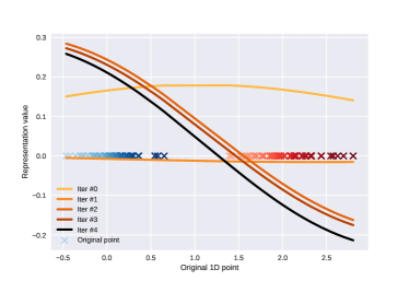
(a) Encoding evolution during fitting

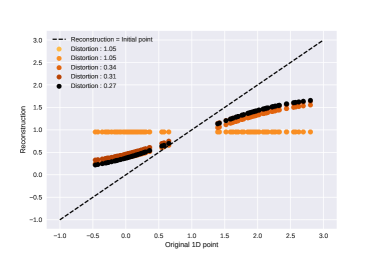
(b) Decoding evolution during fitting

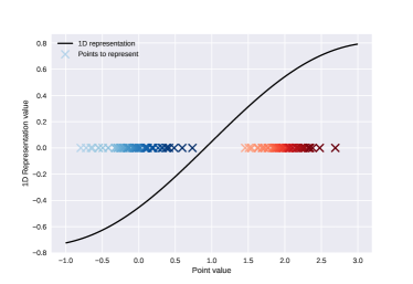
(c) 1D Gaussian clusters and 1D representation

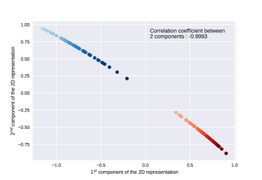
(d) 2D representation of the clusters

Figure 5: Algorithm behavior on 1D data

Figure 6 shows the algorithm’s behavior on Gaussian clusters. Whenever original points and their representations cannot be displayed on the same graph (i.e. when whether the original data or its representation is of dimension more than 2), the colormap helps linking them. In Figure 6(a), the original 2D data are plotted, while Figure 6(b) shows their 1D representations. The colormap has been established according to the value of this representation. First, the two clusters remain well separated in the representation space (positive/negative representations). But what is really interesting is how they are separated. The lighter the blue points are, the most negative representation they have, or in other terms, the most certain they are to be in the blue cluster. Similarly, the darker the red points are, the most positive representation they have. When looking at these points on Figure 6(a), one sees that it matches the distribution: light blue points are the most distant from the red cluster, and conversely for the dark red ones. The algorithm has found the direction that discriminates the two clusters. Similar results are shown for 3 Gaussian clusters on Figure 6(c) and Figure 6(d).

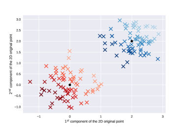
(a) 2D Gaussian clusters

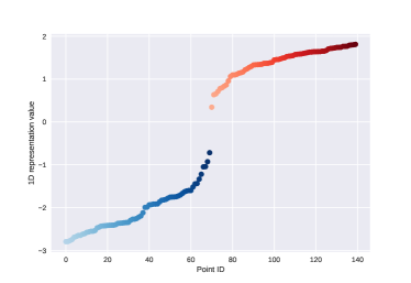
(b) 1D representation of the clusters

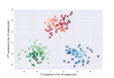
(c) 2D Gaussian clusters (3)

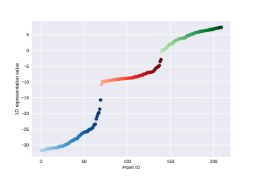
(d) 1D representation of the clusters

Figure 6: Algorithm behavior on Gaussian clusters

Finally, Figure 7 shows the algorithm’s behavior on the so called two moons dataset. 2D original points (Figure 7(a) and Figure 7(c), colored differently according to the representation on their right) are first mapped to a 1D representation (Figure 7(b)). Just as for the 3 concentric circles example, this 1D representation is discriminative, also with intra-cluster variability in order to reconstruct properly. The 2D re-representation on Figure 7(d) shows again the disentangling properties of the KAE.

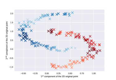
(a) Two moons dataset, colored w.r.t. its 1D representation

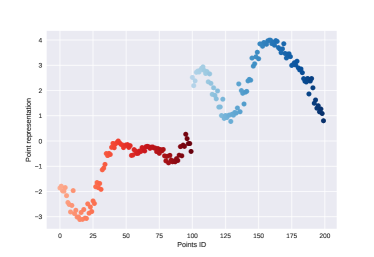
(b) 1D representation of the 2 moons

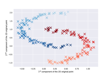
(c) Two moons dataset, colored w.r.t. its 2D representation

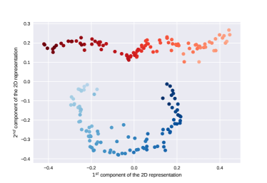
(d) 2D representation of the 2 moons

Figure 7: Algorithm behavior on the 2 moons dataset

C.2 NCI Data

C.2.1 All strategies on 8 cancers graph

C.3 5 strategies on 59 cancers table

Table 3: NMSEs on Molecular Activity for Different Types of Cancer

	KRR	KPCA 10 + RF	KPCA 50 + RF	$\text{K}^{2}$AE 10 + RF	$\text{K}^{2}$AE 50 + RF
Cancer 01	0.02978	0.03279	0.03035	0.03097	0.02808
Cancer 02	0.03004	0.03194	0.02978	0.03099	0.02775
Cancer 03	0.02878	0.03155	0.02914	0.02989	0.02709
Cancer 04	0.03003	0.03274	0.03074	0.03218	0.02924
Cancer 05	0.02954	0.03185	0.02903	0.03065	0.02754
Cancer 06	0.02914	0.03258	0.03083	0.03134	0.02838
Cancer 07	0.03113	0.03468	0.03207	0.03257	0.03018
Cancer 08	0.02899	0.03162	0.02898	0.03065	0.02770
Cancer 09	0.02860	0.02992	0.02804	0.02872	0.02627
Cancer 10	0.02987	0.03291	0.03111	0.03170	0.02910
Cancer 11	0.03035	0.03258	0.03095	0.03188	0.02900
Cancer 12	0.03178	0.03461	0.03153	0.03253	0.02983
Cancer 13	0.03069	0.03338	0.03104	0.03162	0.02857
Cancer 14	0.03046	0.03340	0.03102	0.03135	0.02862
Cancer 15	0.02910	0.03221	0.03066	0.03131	0.02806
Cancer 16	0.02956	0.03220	0.02958	0.03060	0.02779
Cancer 17	0.03004	0.03413	0.03140	0.03145	0.02869
Cancer 18	0.02954	0.03195	0.03005	0.03108	0.02805
Cancer 19	0.03003	0.03211	0.03079	0.03178	0.02832
Cancer 20	0.02911	0.03179	0.03041	0.03085	0.02769
Cancer 21	0.02963	0.03275	0.03023	0.03152	0.02837
Cancer 22	0.03075	0.03391	0.03089	0.03263	0.02958
Cancer 23	0.03006	0.03286	0.02983	0.03109	0.02760
Cancer 24	0.03075	0.03398	0.03112	0.03242	0.02894
Cancer 25	0.02977	0.03307	0.03054	0.03159	0.02824
Cancer 26	0.03083	0.03358	0.03132	0.03206	0.02959
Cancer 27	0.03083	0.03347	0.03116	0.03230	0.02974
Cancer 28	0.03061	0.03256	0.03116	0.03185	0.02918
Cancer 29	0.03056	0.03360	0.03147	0.03181	0.02892
Cancer 30	0.03099	0.03288	0.03100	0.03181	0.02906
Cancer 31	0.03082	0.03361	0.03161	0.03242	0.02986
Cancer 32	0.03233	0.03562	0.03300	0.03422	0.03158
Cancer 33	0.03065	0.03208	0.03045	0.03142	0.02909
Cancer 34	0.03326	0.03668	0.03423	0.03486	0.03183
Cancer 35	0.03292	0.03587	0.03393	0.03450	0.03146
Cancer 36	0.03068	0.03389	0.03122	0.03249	0.02925
Cancer 37	0.03023	0.03310	0.03061	0.03130	0.02878
Cancer 38	0.03100	0.03487	0.03156	0.03327	0.02974
Cancer 39	0.02989	0.03288	0.03149	0.03148	0.02865
Cancer 40	0.03166	0.03525	0.03201	0.03352	0.03010
Cancer 41	0.03139	0.03501	0.03203	0.03316	0.03025
Cancer 42	0.03010	0.03251	0.03013	0.03072	0.02807
Cancer 43	0.03042	0.03324	0.03062	0.03144	0.02806
Cancer 44	0.02838	0.03045	0.02821	0.02927	0.02679
Cancer 45	0.02910	0.03085	0.02895	0.02970	0.02651
Cancer 46	0.02969	0.03258	0.02996	0.03111	0.02834
Cancer 47	0.03148	0.03438	0.03346	0.03286	0.03056
Cancer 48	0.03272	0.03640	0.03397	0.03425	0.03197
Cancer 49	0.03305	0.03392	0.03329	0.03334	0.03148
Cancer 50	0.03229	0.03637	0.03300	0.03404	0.03155
Cancer 51	0.02943	0.03188	0.03028	0.03072	0.02857
Cancer 52	0.03309	0.03420	0.03252	0.03335	0.03130
Cancer 53	0.03170	0.03340	0.03105	0.03170	0.02843
Cancer 54	0.03189	0.03439	0.03164	0.03345	0.03036
Cancer 55	0.03082	0.03339	0.03146	0.03207	0.02892
Cancer 56	0.03026	0.03327	0.03041	0.03185	0.02901
Cancer 57	0.02962	0.03237	0.02990	0.03162	0.02855
Cancer 58	0.02883	0.03200	0.02978	0.03058	0.02783
Cancer 59	0.02936	0.03208	0.02914	0.03032	0.02750

References

- Alain and Bengio, (2014) Alain, G. and Bengio, Y. (2014). What regularized auto-encoders learn from the data-generating distribution. J. Mach. Learn. Res., 15(1):3563–3593.
- Álvarez et al., (2012) Álvarez, M. A., Rosasco, L., and Lawrence, N. D. (2012). Kernels for vector-valued functions: A review. Foundations and Trends in Machine Learning, 4(3):195–266.
- Baldi, (2012) Baldi, P. (2012). Autoencoders, unsupervised learning, and deep architectures. In Proceedings of ICML Workshop on Unsupervised and Transfer Learning, pages 37–49.
- Bauschke et al., (2011) Bauschke, H. H., Combettes, P. L., et al. (2011). Convex analysis and monotone operator theory in Hilbert spaces, volume 408. Springer.
- Bengio et al., (2013) Bengio, Y., Courville, A., Vincent, P., and Umanità, V. (2013). Representation learning: a review and new perspectives. IEEE transactions on pattern analysis and machine intelligence, 35(8):1798–1828.
- Bourlard and Kamp, (1988) Bourlard, H. and Kamp, Y. (1988). Auto-association by multilayer perceptrons and singular value decomposition. Biological cybernetics, 59(4):291–294.
- (7) Brouard, C., Shen, H., Dührkop, K., d’Alché-Buc, F., Böcker, S., and Rousu, J. (2016a). Fast metabolite identification with input output kernel regression. Bioinformatics, 32(12):28–36.
- (8) Brouard, C., Szafranski, M., and d’Alché-Buc, F. (2016b). Input output kernel regression: Supervised and semi-supervised structured output prediction with operator-valued kernels. Journal of Machine Learning Research, 17:176:1–176:48.
- Caponnetto et al., (2008) Caponnetto, A., Micchelli, C. A., , M., and Ying, Y. (2008). Universal multitask kernels. Journal of Machine Learning Research, 9:1615–1646.
- Chollet et al., (2015) Chollet, F. et al. (2015). Keras, https://keras.io.
- Gholami and Hajisami, (2016) Gholami, B. and Hajisami, A. (2016). Kernel autoencoder for semi-supervised hashing. In Applications of Computer Vision (WACV), 2016 IEEE Winter Conference on, pages 1–8. IEEE.
- Kadri et al., (2016) Kadri, H., Duflos, E., Preux, P., Canu, S., Rakotomamonjy, A., and Audiffren, J. (2016). Operator-valued kernels for learning from functional response data. Journal of Machine Learning Research, 17:20:1–20:54.
- Kampffmeyer et al., (2017) Kampffmeyer, M., Løkse, S., Bianchi, F. M., Jenssen, R., and Livi, L. (2017). Deep kernelized autoencoders. In Scandinavian Conference on Image Analysis, pages 419–430. Springer.
- Kipf and Welling, (2016) Kipf, T. N. and Welling, M. (2016). Variational graph autoencoders. NIPS Workshop on Bayesian Deep Learning.
- Ledoux and Talagrand, (1991) Ledoux, M. and Talagrand, M. (1991). Probability in Banach Spaces: Isoperimetry and Processes. Springer Science & Business Media.
- Maurer, (2014) Maurer, A. (2014). A chain rule for the expected suprema of gaussian processes. In Algorithmic Learning Theory: 25th International Conference, ALT 2014, Bled, Slovenia, October 8-10, 2014, Proceedings, volume 8776, page 245. Springer.
- Maurer, (2016) Maurer, A. (2016). A vector-contraction inequality for rademacher complexities. In International Conference on Algorithmic Learning Theory, pages 3–17. Springer.
- Maurer and Pontil, (2016) Maurer, A. and Pontil, M. (2016). Bounds for vector-valued function estimation. arXiv preprint arXiv:1606.01487.
- Micchelli and Pontil, (2005) Micchelli, C. A. and Pontil, M. (2005). On learning vector-valued functions. Neural computation, 17(1):177–204.
- Mohri et al., (2012) Mohri, M., Rostamizadeh, A., and Talwalkar, A. (2012). Foundations of Machine Learning. MIT press.
- Pedregosa et al., (2011) Pedregosa, F. et al. (2011). Scikit-learn: Machine learning in Python. Journal of Machine Learning Research, 12:2825–2830.
- Pisier, (1986) Pisier, G. (1986). Probabilistic methods in the geometry of banach spaces. In Probability and analysis, pages 167–241. Springer.
- Salakhutdinov and Hinton, (2009) Salakhutdinov, R. and Hinton, G. (2009). Deep boltzmann machines. In van Dyk, D. and Welling, M., editors, Proceedings of the Twelth International Conference on Artificial Intelligence and Statistics, volume 5 of Proceedings of Machine Learning Research, pages 448–455. PMLR.
- Schölkopf et al., (1997) Schölkopf, B., Smola, A., and Müller, K.-R. (1997). Kernel principal component analysis. In International conference on artificial neural networks, pages 583–588. Springer.
- Schölkopf et al., (1998) Schölkopf, B., Smola, A., and Müller, K.-R. (1998). Nonlinear component analysis as a kernel eigenvalue problem. Neural computation, 10(5):1299–1319.
- Senkene and Tempel’man, (1973) Senkene, E. and Tempel’man, A. (1973). Hilbert spaces of operator-valued functions. Lithuanian Mathematical Journal, 13(4):665–670.
- Smola and Schölkopf, (1998) Smola, A. J. and Schölkopf, B. (1998). Learning with kernels, volume 4. Citeseer.
- Smola and Schölkopf, (2000) Smola, A. J. and Schölkopf, B. (2000). Sparse greedy matrix approximation for machine learning.
- Su et al., (2010) Su, H., Heinonen, M., and Rousu, J. (2010). Structured output prediction of anti-cancer drug activity. In Dijkstra, T., Tsivtsivadze, E., Marchiori, E., and Heskes, T., editors, Pattern Recognition in Bioinformatics - 5th IAPR International Conference, PRIB 2010, Proceedings, volume 6282 of Lecture Notes in Computer Science, pages 38–49. Springer.
- Vincent et al., (2010) Vincent, P., Larochelle, H., Lajoie, I., Bengio, Y., and Manzagol, P.-A. (2010). Stacked denoising autoencoders: Learning useful representations in a deep network with a local denoising criterion. J. Mach. Learn. Res., 11:3371–3408.