Particle-based simulations of reaction-diffusion processes with Aboria

Abstract

Mathematical models of transport and reactions in biological systems have been traditionally written in terms of partial differential equations (PDEs) that describe the time evolution of population-level variables. In recent years, the use of stochastic particle-based models, which keep track of the evolution of each organism in the system, has become widespread. These models provide a lot more detail than the population-based PDE models, for example by explicitly modelling particle-particle interactions, but bring with them many computational challenges. In this paper we overview Aboria, a powerful and flexible C++ library for the implementation of numerical methods for particle-based models. We demonstrate the use of Aboria with a commonly used model in mathematical biology, namely cell chemotaxis. Cells interact with each other and diffuse, biased by extracellular chemicals, that can be altered by the cells themselves. We use a hybrid approach where particle-based models of cells are coupled with a PDE for the concentration of the extracellular chemical.

1 Introduction

Biology has recently experienced a revolution through the development of new, quantitative, measurement techniques. As an example, super-resolution microscopy allows biomolecules to be localised, counted and distinguished (Betzig et al, 2006). Traditional modelling approaches using partial differential equations (PDEs) for population-level variables (concentrations, densities) are unable to capture and explain some of the particle-level (for example, molecule- or cell-level) features that we are now obtaining from experiments. This is why a more detailed modelling approach, namely particle-based or agent-based models that describe the behaviour of each organism, is now increasingly used by the mathematical biology community. Computer simulations are ideal for studying the dynamical mechanisms arising from the interplay of these particles, filling in the details that cannot be resolved experimentally, and testing/generating biological hypothesis. These simulations comprise algorithms for particle-based stochastic reaction-diffusion processes that track individual particles and are computationally expensive.

The computational requirements of particle-based models, such as the efficient calculation of interactions between particles, are challenging to implement in a way that scales well with the number of particles, uniform and non-uniform particle distributions, different spatial dimensions and periodicity. The majority of existing software is typically designed to suit a particular application, and therefore tends not to be sufficiently generic that can be used to implement these computationally challenging routines, and so they are reimplemented again and again in each software package.

The primary class of software for particle-based methods is geared towards molecular dynamics simulations, such as the hugely popular GROMACS (Abraham et al, 2015), or OpenMM (Eastman et al, 2012) packages. These generally include sophisticated neighbour searching and evaluation of long-range forces, but do not include the possibility of reactions between particles, a vital component of many biological models. On the other hand, the biochemical simulator package Smoldyn (Andrews and Bray, 2004) implements both unimolecular and bimolecular reactions using the Smoluchowski method, but has limited capabilities to implement interactions between particles and transport mechanisms other than unbiased Brownian motion.

Aboria is a C++ library for the numerical implementation of particle-based models (Robinson and Bruna, 2017). Aboria aims to provide a general purpose library that allows the user complete control to define whatever interactions they wish on a given particle set, while implementing efficiently the difficult algorithmic aspects of particle-based methods, such as neighbourhood searches and the calculation of long-range forces. It is agnostic to any particular numerical method, for example it does not contain any particular molecular dynamics or Smoluchowski dynamics algorithms, but instead provides the user with computational tools that allow them to implement these algorithms in a customised fashion. It is thus especially suitable for the implementation of novel particle-based methods, or hybrid models that couple particle-based models with continuum PDE models. In particular, Aboria gives the user:

1. A container class to store a particle set with a position and unique id for each particle, as well as any number of user-defined variables associated to each particle with arbitrary types (for example, to store a velocity, a force, or the particle size).

2. The ability to embed each particle set within an $n$-dimensional hypercube with arbitrary periodicity. The underlying data structure can be a cell list, kd-tree or hyper oct-tree. The data structure can be chosen to suit the particular application.

3. Flexible neighbourhood queries that return iterators, and can use any integer $p$-norm distance measure (for example, the Euclidean distance is given by $p=2$, the Chebyshev distance is given by $p=\infty$).

4. The ability to calculate long-range forces between $N$ particles efficiently (that is, in $O(N)$) using the black-box fast multipole method (Fong and Darve, 2009). This method can be used for any long-range force that is well-approximated by a low-order polynomial for large distances between particles (the computational cost of the model scales with the degree of the polynomial).

5. An easy to use embedded Domain Specific Language (eDSL) expressing a wide variety of particle-particle interactions. For specialised cases which cannot be easily expressed by this symbolic eDSL, Aboria also provides a low-level interface based on the C++ Standard Template Library (Stroustrup, 2013).

The aim of this paper is to demonstrate how Aboria can be used to implement many features of particle-based models common in mathematical biology. These include heterogeneous particle populations, interactions between particles, volume exclusion, biased transport, reactions, and proliferation. We showcase the many features of the Aboria library through a well-known model in mathematical biology, namely cell chemotaxis. In Sect. 2 we detail the mathematical model for chemotaxis. Then in Sect. 3 we show a step-by-step implementation of the model with Aboria. Finally, we show how to output and analyse the data using Python in Sect. 4.

2 Model for chemotaxis

As our guiding example, we consider chemotactic cell migration with volume exclusion. In particular, we study a population of $N$ cells divided into two sub-populations (types $\alpha$ and $\beta$) and a diffusing attractive chemical substance that is produced by cells of type $\alpha$ and consumed by cells of type $\beta$. Cells move around in a two-dimensional domain $\Omega$ due to Brownian motion, biased by gradients in the concentration of the chemical in the case of type $\beta$ cells. Cells can also undergo reactions that change their type from chemical producers to chemical consumers. Volume exclusion can be modelled by either point particles with a short-range repulsive interaction potential $u$ (so that cells are allowed to deform if in close contact) or hard-sphere particles that are not allowed to overlap. To make the example as broad as possible, we take a hybrid modelling approach whereby the cells are modelled discretely using particle-based models for Brownian motion, while the chemical is represented by its concentration $c$ using a reaction-diffusion PDE. Hybrid models of chemotaxis have been considered in Guo et al (2008); Dallon and Othmer (1997); Franz and Erban (2013); Newman and Grima (2004); McLennan et al (2012).

Let ${\bf X}_{i}(t)$ denote the position of the $i$th particle in $\Omega\subset\mathbb{R}^{2}$. Let $S_{\alpha}(t)$ denote the set of cells of type $\alpha$ and $S_{\beta}(t)$ denote the set of cells of type $\beta$ at time $t$. For each particle, the motion through space is described by a stochastic differential equation (SDE). For $i\in S_{\alpha}(t)$,

$$\mathrm{d}{\bf X}_{i}(t)=\sqrt{2D_{\alpha}}\mathrm{d}{\bf W}_{i}(t)-\sum_{j\neq i}\nabla_{i}u(\|{\bf X}_{i}(t)-{\bf X}_{j}(t)\|)\mathrm{d}t,$$ (1a)

where $D_{\alpha}$ is the diffusion coefficient of cells of type $\alpha$, and $\nabla_{i}$ denotes the gradient with respect to ${\bf X}_{i}$. For $i\in S_{\beta}(t)$

$$\mathrm{d}{\bf X}_{i}(t)=\sqrt{2D_{\beta}}\mathrm{d}{\bf W}_{i}(t)+\chi\nabla c({\bf X}_{i}(t),t)\mathrm{d}t-\sum_{j\neq i}\nabla_{i}u(\|{\bf X}_{i}(t)-{\bf X}_{j}(t)\|)\mathrm{d}t.$$ (1b)

Here $D_{\beta}$ is the diffusion coefficient of cells of type $\beta$, $\chi$ denotes the chemotactic sensitivity of the cells (taken to be constant) and $c({\bf x},t)$ is the concentration of chemical at position ${\bf x}$ and time $t$. The interaction potential $u$ may be a soft potential incorporating effects such as size exclusion by cells and cell-cell adhesion. Typical examples are a Morse potential (D’Orsogna et al, 2006; Middleton et al, 2014), an exponential potential (Bruna et al, 2017), or a Lennard-Jones potential (Jeon et al, 2010). Alternatively, the interaction between cells may be modelled as a singular hard-sphere potential so that cells are not allowed to overlap each other, for example assuming cells have diameter $\epsilon$ and taking $u(r)=+\infty$ for $r<\epsilon$, $u(r)=0$ otherwise would impose that $\|{\bf X}_{i}(t)-{\bf X}_{j}(t)\|\geq\epsilon$ for all $t$ (Bruna and Chapman, 2012). Also, cells can change type according to the following reactions:

$$\alpha\xrightarrow{r_{\alpha}}\beta,\qquad\beta\xrightarrow{r_{\beta}(c)}\alpha.$$ (1c)

Cells of type $\alpha$ change to type $\beta$ with constant rate $r_{\alpha}$, whereas cells of type $\beta$ change type with rate $r_{\beta}(c(X_{\beta}(t),t))$, where $X_{\beta}(t)$ is the position of the type $\beta$ cell (that is, the rate may depend on the chemical concentration at the location of the cell).

Finally, cells of type $\alpha$ secrete chemoattractant at a constant rate $k_{\alpha}$, while cells of type $\beta$ consume it at a constant rate $k_{\beta}$. The chemical diffuses with a diffusion constant $D_{c}$ and degrades with rate $\gamma$. The chemical concentration $c({\bf x},t)$ evolves according to the PDE

$$\partial_{t}c=D_{c}\nabla^{2}c+k_{\alpha}\rho_{\alpha}^{\delta}({\bf x},t)-k_{\beta}\rho_{\beta}^{\delta}({\bf x},t)c-\gamma c,$$ (1d)

where $\rho_{\alpha}^{\delta}$ and $\rho_{\beta}^{\delta}$ denote the random measures for the density of cells of type $\alpha$ and $\beta$, respectively,

$$\rho_{\alpha}^{\delta}({\bf x},t)=\sum_{i\in S_{\alpha}(t)}\delta({\bf x}-{\bf X}_{i}(t)),\quad\rho_{\beta}^{\delta}({\bf x},t)=\sum_{i\in S_{\beta}(t)}\delta({\bf x}-{\bf X}_{i}(t)).$$ (1e)

The SDEs (1a) and (1b) and the PDE (1d) are complemented with suitable initial conditions and either periodic or no-flux boundary conditions).

The numerical implementation of model (1) is challenging for several reasons. In the remainder of this section we go through each of the problems one faces. In addition to the points below, it is worth keeping in mind that generally we are interested in statistical averages of the simulations (in order to compare them with, for example, experiments or continuum PDE models). As a result, it is crucial that the simulation method is implemented efficiently, exploiting parallelisation and other algorithms to speed up the simulation.

2.1 Time-stepping for diffusion and reactions

The standard way to numerically integrate the SDEs (1a) and (1b) is to use a fixed time-step $\Delta t$ and a Euler–Maruyama discretisation. For (1a), this reads

$${\bf X}_{i}(t+\Delta t)={\bf X}_{i}(t)+\sqrt{2D_{\alpha}\Delta t}\xi_{i}-\sum_{j\neq i}\nabla_{i}u(\|{\bf X}_{i}(t)-{\bf X}_{j}(t)\|)\Delta t,$$ (2)

where $\xi_{i}$ is a two-dimensional normally distributed random variable with zero mean and unit variance. Reactions (1c) can also be simulated using a fixed time-step. For example, if $N_{\alpha}(t)$ is the number of $\alpha$-type cells at time $t$, then the first reaction occurs during $[t,t+\Delta t)$ if $\zeta<N_{\alpha}(t)r_{\alpha}\Delta t$, where $\zeta$ is a uniformly distributed random number, $\zeta\sim U(0,1)$.

The downside of the fixed time-stepping approach to simulating reactions is that: (i) the time-step must be chosen to ensure that $N_{\alpha}(t)r_{\alpha}\Delta t\ll 1$, which imposes a restriction on the size of $\Delta t$; (ii) choosing such a small $\Delta t$ means that in most time-steps no reactions will take place. Hence, lots of random numbers $\zeta$ need to be generated before the reaction takes place (Erban et al, 2007); (iii) there is an exact and more efficient simulation algorithm, the Gillespie algorithm (Gillespie, 1977). The Gillespie algorithm computes the time $t+\Delta t$ that the next reaction will occur as $\Delta t=\ln(1/\zeta)/(N_{\alpha}(t)r_{\alpha})$, where $\zeta\sim U(0,1)$ again.

In lattice-based models for reaction-diffusion processes, space is discretised into a regular lattice and diffusion is represented as jumps between neighbouring lattices, and can be treated a reaction events. This implies that both reactions and diffusion can be implemented using the same framework, the Gillespie algorithm being the obvious choice. In contrast, off-lattice Brownian motion models such as (1a) and (1b) do not fit this framework and are naturally implemented with a fixed time-step approach (2). As a result, the simulation algorithm is either of fixed time-step $\Delta t$ for both processes, where $\Delta t$ is small enough to resolve diffusion, reactions, and interactions well (see Subsec. 2.2), or fixed time-step for the cell position updates and variable time-step for the cell number updates.

2.2 Cell-cell interactions

Pairwise interactions between $N$ particles will generally lead to an $O(N^{2})$ loop to compute the interaction terms in (1a) and (1b) at every time-step $\Delta t$. If the interaction potential $u$ is short ranged, it is convenient to use neighbourhood searches as we only need to evaluate the distances and forces between particles that are close enough. This reduces the computational cost to $O(aN)$, where $a$ is the typical number of particles in the neighbourhood of one particle.

For long-range forces, neighbourhood searches do not help as every particle interacts significantly with every other particle. However, in many commonly used interactions forces (for example, electrostatics, gravitational) the interactions between well-spaced clusters of particles can be efficiently approximated by means of the fast multipole method (FMM) (Greengard and Rokhlin, 1987), which also leads to a total computational cost of $O(N)$. Aboria implements a version of the black-box FMM (Fong and Darve, 2009), which uses Chebyshev interpolation to approximate the interaction of well-separated clusters. Since the present chemotaxis model uses short-range interactions (to represent cell volume exclusion), we do not discuss the FMM further in this paper. For more information of Aboria’s FMM capabilities, the reader is referred to the documentation.

Interactions between particles also require a careful choice of $\Delta t$ so that they are well resolved. If $\Delta t$ is too large, interactions between Brownian steps might be missed. A good rule of thumb is that the mean relative displacement (ignoring any drift terms) between two particles with diffusion coefficients $D_{i}$ and $D_{j}$ respectively, $\sqrt{2(D_{i}+D_{j})\Delta t}$, should be less than the range of the interaction potential (equal to the sum of the particles’ radii in the case of a hard-sphere interaction). It is not uncommon for short-range potentials to be singular or very steep at the origin. In these cases, the scheme (2) may not resolve well the original SDE (1a) unless the time-step $\Delta t$ is prohibitively small (so that the drift term in (2) does not send particles very far apart, possibly missing other interactions on the way). An alternative to the explicit Euler–Maruyama scheme (2) is to use an implicit scheme with better convergence properties, or the so-called tamed Euler scheme (Hutzenthaler et al, 2012), which modifies the drift term of (1a), $f_{i}(\vec{X}(t))=\sum_{j\neq i}\nabla_{i}u(\|{\bf X}_{i}(t)-{\bf X}_{j}(t)\|)$, where $\vec{X}=({\bf X}_{1},\dots,{\bf X}_{N})$, so that it is uniformly bounded by one:

$${\bf X}_{i}(t+\Delta t)={\bf X}_{i}(t)+\sqrt{2D_{\alpha}\Delta t}\xi_{i}-\frac{f_{i}(\vec{X}(t))\Delta t}{1+\|f_{i}(\vec{X}(t))\|\Delta t}.$$ (3)

This scheme coincides with the Euler–Maruyama scheme (2) up to order $\Delta t$ and it is just as simple to implement, but it has the advantage of allowing larger simulation time-steps for (1a) with repulsive potentials singular at the origin.

In the case of a hard-sphere interaction potential, there are several options to implement the collisions between particles (see Bruna, 2012, p. 33). One option is to update particle positions according to (2) and correct any overlap at time $t+\Delta t$ by moving particles apart in the direction along the line joining the two particle centres. Namely, if the distance between two particles is $d_{ij}=\|{\bf X}_{i}(t+\Delta t)-{\bf X}_{j}(t+\Delta t)\|<(\epsilon_{i}+\epsilon_{j})/2$, where $\epsilon_{i}$ is the diameter of the $i$th particle, then the particles are moved apart a distance $2d_{p}$, where $d_{p}=(\epsilon_{i}+\epsilon_{j})/2-d_{ij}$ is the distance that particles have penetrated each other illegally. Note that we use twice this distance to account for the fact that particles would have collided and moved apart by $d_{p}$ (moving them apart only by $d_{p}$ would make them be exactly in contact). The way the total update distance is distributed among particles depends on the mean travelled distance of each particle and their diffusion coefficients. If the particles are of the same type, then the distance is shared equally among them. If instead one particle is immobile (suppose it is a fixed obstacle), then the total displacement is imposed on the other particle. In general, if the particles have diffusion coefficients $D_{i}$ and $D_{j}$, the $i$th particle takes $D_{i}/(D_{i}+D_{j})$ of the displacement, and the rest goes to particle $j$.

Another method to implement hard-sphere collisions is known as the elastic collision method (Scala et al, 2007). It consists of an event-driven algorithm between Brownian time-steps of length $\Delta t$, whereby each Brownian particle is attributed a “velocity” $V_{i}(t)=({\bf X}_{i}(t+\Delta t)-{\bf X}_{i}(t))/\Delta t$ and collisions between all particles in the interval $[t,t+\Delta t)$ are predicted and treated using a standard event-driven method for ballistic dynamics. On the one hand, this method predicts rather than corrects collisions, and it is therefore more accurate than the first one. This implies that one may take larger steps $\Delta t$. On the other hand, the event-driven method is computationally more intensive and is more complex to implement.

2.3 Spatial matching between discrete and continuous variables

The hybrid model (1) combines two modelling frameworks: a particle-based approach for the cells, equations (1a) and (1b), and a continuum approach for the chemical concentration, (1d). This means that we have to consider each part of the model separately and establish a way to match them in space.

One approach is that taken by Newman and Grima (2004), where the chemical concentration $c({\bf x},t)$ is found by formally integrating equation (1d) along the cell paths. Assuming $\Omega=\mathbb{R}^{2}$, the result is

$$c({\bf x},t)=\int_{0}^{t}\int_{\mathbb{R}^{2}}G_{\gamma}({\bf x}-{\bf x}^{\prime},t-t^{\prime})\left[k_{\alpha}\rho_{\alpha}^{\delta}({\bf x}^{\prime},t^{\prime})-k_{\beta}\rho_{\beta}^{\delta}({\bf x}^{\prime},t^{\prime})\right]\mathrm{d}x^{\prime}\mathrm{d}t^{\prime},$$ (4)

where $\rho_{\alpha}^{\delta}$ and $\rho_{\alpha}^{\delta}$ are given in (1e) and $G_{\gamma}$ is the Green’s function for the chemical diffusion equation in $\mathbb{R}^{2}$,

$$G_{\gamma}({\bf x},t)=(4\pi D_{c}t)^{-1}\exp\left(-\frac{\|{\bf x}\|^{2}}{4D_{c}t}-\gamma t\right).$$ (5)

Since we have an explicit expression for the chemical concentration in the whole space, the chemical gradient in (1b) and the chemical concentration in the reaction rate in (1c) can be evaluated exactly. In particular, the gradient in (1b) can be written as

$$\nabla c({\bf X}_{i}(t),t)=\int_{0}^{t}\Big{[}\sum_{j\in S_{\alpha}(t^{\prime})}k_{\alpha}\nabla G_{\gamma}({\bf X}_{i}(t)-{\bf X}_{j}(t^{\prime}),t-t^{\prime})\\ -\sum_{j\in S_{\beta}(t^{\prime})}k_{\beta}\nabla G_{\gamma}({\bf X}_{i}(t)-{\bf X}_{j}(t^{\prime}),t-t^{\prime})\Big{]}\mathrm{d}t^{\prime}.$$ (6)

Therefore, this approach requires the history of the cell positions ${\bf X}_{i}(t)$ only, and no explicit evaluation of the chemical concentration (unless $c$ is required as a simulation output, in which case one uses (4)). One major drawback of this approach is that it only works when the domain $\Omega$ is the whole space, and therefore it may not be applicable in many cases.

The alternative approach is to discretise and integrate the chemical concentration on a grid, for example using a finite-differences method. This approach works for bounded domains, but it has the disadvantage that it requires spatial matching between the discrete and continuum variables. Specifically, the particles can be positioned at an arbitrary point inside the domain, while the chemical concentration is only calculated at grid points ${\bf p}_{1},\dots,{\bf p}_{L}\in\Omega$. Then we have a two-way matching to do: interpolate the concentration at the off-grid particle positions to simulate (1b) and (1c), and generate estimates for the cell densities $\rho_{\alpha}^{\delta}$ and $\rho_{\beta}^{\delta}$ at the points ${\bf p}_{l}$ to integrate (1d).

The approximation of $c({\bf x},t)$ and $\nabla c({\bf x},t)$ at points ${\bf X}_{i}(t)$ can be done using a variety of interpolation methods, such as linear or spline interpolation. Since the grid points ${\bf p}_{l}$ on which $c$ is computed are chosen beforehand to provide a good approximation of $c$, they will generally also form a good set of interpolating points (Franz and Erban, 2013).

The interpolation of the cell densities $\rho_{\alpha}^{\delta}$ and $\rho_{\beta}^{\delta}$ from the cell positions ${\bf X}_{i}$ to the grid points ${\bf p}_{l}$, necessary to update $c({\bf p}_{l},t)$ according to (1d), is slightly more delicate. A basic approach would be to “shift” the delta function from ${\bf X}_{i}$ to its closest grid point ${\bf p}_{l}$, so that $\rho_{\alpha}^{\delta}({\bf p}_{l},t)$ is a count of the number of $\alpha$-type cells in the neighbourhood of ${\bf p}_{l}$. However, this is quite a crude approximation to make, rendering the more accurate approaches in the discretisation of the equations or the interpolation of $c$ a waste of effort. This is why the standard approach is to obtain a continuous approximation of the density, or density estimate, and then evaluate it at the grid points ${\bf p}_{l}$. One way to achieve this is to use a particle-in-cell method with piecewise linear polynomials as done by Dallon and Othmer (1997). They use a square lattice and the mass of a delta function at ${\bf X}_{i}$ is distributed among the four nearest grid points proportionally to their distances. Another way is to use a kernel density estimation, which is generally used to estimate the probability density of a random process from a large number of iterations (for details see Franz and Erban, 2013). The estimate of the density of type $\alpha$ cells is found as

$$\rho_{\alpha}({\bf x},t)=\sum_{i\in S_{\alpha}(t)}K_{h}({\bf x}-{\bf X}_{i}(t))=K_{h}({\bf x})\ast\rho_{\alpha}^{\delta}({\bf x},t),$$ (7)

where $\ast$ is the spatial convolution, and $K_{h}({\bf x})$ denotes a kernel of bandwidth $h$, $K_{h}({\bf x})=h^{-2}K({\bf x}/h)$, taken to be a continuous, symmetric and normalised function. The idea is that, as the bandwidth parameter $h\to 0$, the estimate $\rho_{\alpha}$ approximates the sum of delta functions in $\rho_{\alpha}^{\delta}$. The Gaussian kernel, $K({\bf x})=(2\pi)^{-1}\exp(-\|{\bf x}\|^{2}/2)$, is one of the most commonly used kernels for density estimation. In the context of hybrid modelling, the Gaussian kernel density estimation was used in Franz et al (2013); McLennan et al (2012).

The earliest hybrid models for chemotaxis modelled cells as point particles. Accordingly, the formulation of (1d) with Dirac deltas was considered to be the exact model, and the kernel density estimation its approximation. However, if the actual size of cells is taken into account, it makes sense to assume that the cells consume or degrade chemical all along their shape, and not only in the centre. In this case, the bandwidth parameter $h$ can be thought of the lengthscale of the cell (for example, $h$ can be related to the hard-sphere diameter when cells are modelled as hard bodies), independent of the grid spacing for the chemical (McLennan et al, 2012).

3 Model implementation with Aboria

We consider an example in a square domain, $\Omega=[-L/2,L/2]^{2}$, with no-flux boundary conditions. Cells interact with each other via a soft short-range repulsive potential $u(r)=\exp(-r/\epsilon)$, with $\epsilon=0.01$. Initially there are the same number of particles of each type, $N_{\alpha}=N_{\beta}$, and $N=N_{\alpha}+N_{\beta}$. Cells of type $\alpha$ are distributed according to a two-dimensional normal centred at the origin and $\sigma=0.1$. Cells of type $\beta$ are uniformly distributed in the whole domain. Initially there is no chemical in the domain.

3.1 Particle set with two types of particles

We define three Aboria variables: type to refer to the cell type (type=true for cells of type $\alpha$, and type=false for cells of type $\beta$), concentration for the concentration of $c$ at the location of the particle, and drift to store the two-dimensional drift vector $\chi\nabla c$ (using an Aboria vdouble2 type, representing a two-dimensional vector). We then define the particle set type, given by Particles_t, which contains the Aboria variables and has a spatial dimension of two (specified by the second template argument). For convenience, we also define position as the Particles_t::position subclass (we will use this later on):

⬇

ABORIA_VARIABLE(conc, double, "conc");

ABORIA_VARIABLE(drift, vdouble2, "drift");

ABORIA_VARIABLE(starting, vdouble2, "starting_position");

ABORIA_VARIABLE(next_position, vdouble2, "next␣position");

ABORIA_VARIABLE(type, uint8_t, "type");

typedef Particles<std::tuple<type, drift, conc, starting, next_position>, 2>

Particles_t;

typedef typename Particles_t::position position;

Finally we create particles, an instance of Particles_t, containing $N$ particles, and initialise the random seed of the set based on a unique sample number sample:

⬇

Particles_t particles(N);

particles.set_seed(N * sample);

In Aboria there are two ways to access and operate on particles, either in low-level language or a high-level symbolic language. We show how these two approaches work when initialising the positions of the $N$ particles. The low-level approach uses the standard C++ random library to generate the gaussian and normal distributions, and loops over the particles to set their positions. We define min and max as vectors representing respectively the lower and upper boundaries for each dimension, min $=(-L/2,-L/2)$ and max$=(L/2,L/2)$:

⬇

std::uniform_real_distribution<double> uniform(min[0], max[0]);

std::normal_distribution<double> normal(0, 0.1 * (max[0] - min[0]));

for (size_t i = 0; i < N; ++i) {

get<type>(particles)[i] = i < Na;

auto &gen = get<generator>(particles)[i];

if (get<type>(particles)[i]) {

get<position>(particles)[i] = vdouble2(normal(gen), normal(gen));

} else {

get<position>(particles)[i] = vdouble2(uniform(gen), uniform(gen));

}

}

For the high-level symbolic approach, we define symbolic objects x and typ, representing the position and type variables (and others that we will use later on). We also define two Aboria random number generators; normal for normally distributed numbers, and uni for uniformly distributed numbers. Finally, we also create a label object k associated to the particle set. This label performs a similar function to the $i$ subscript for the variable ${\bf X}_{i}(t)$ in Eq. 2. All operations involving k are implicitly performed over the entire particle set.

⬇

Symbol<position> x;

Symbol<type> typ;

VectorSymbolic<double, 2> vector;

Normal normal;

Uniform uni;

Label<0, Particles_t> k(particles);

Then the high-level initialisation of the positions of particles (assuming that the type variable has already been set) is:

⬇

const double sigma = 0.1 * (max[0] - min[0]);

const double width = max[0]-min[0];

x[k] = if_else(typ[k]

, sigma * vector(normal[k], normal[k])

, width * vector(uni[k], uni[k]) + min);

The advantage of the high-level approach is that we can directly write expressions which are meant to be evaluated over the whole particle set. However, as it implements a custom eDSL, it is by definition limited to operations that can be expressed by this language. For example, the interaction between the chemical grid and the individual particles cannot be expressed with this DSL. Therefore, for the remainder of this paper we will proceed by implementing the model using the lower level interface.

Finally, we initialise the spatial search data structure, providing it with lower (min) and upper (max) bounds for the domain, and setting non-periodic boundary conditions (periodic in this case is false):

⬇

particles.init_neighbour_search(min, max, vbool2::Constant(periodic));

This subdivides the computational domain into square cells of equal size. The default cell side length is such that, if particles were uniformly distributed in the domain, then there would be on average ten particles per cell. However, it is also possible to specify a desired side length as a forth parameter (to make it equal, for example, to a cut-off distance for the calculation of interaction forces).

3.2 Equation of motion of cells

Here we explain how to implement the SDEs (1a) and (1b). For simplicity, in this section we are going to assume that the chemical drift $\chi\nabla c$ in (1b) is fixed and already stored in the drift variable within each $\beta$-particle. To implement the interaction force between two particles ${\bf X}_{i}$ and ${\bf X}_{j}$, we use the euclidean_search function in Aboria, which returns an iterator j that iterates through all the particles within a certain radius (cutoff) of a given point. For each potential pair of particles, the iterator j can provide the shortest vector between $i$ and $j$ (normally ${\bf X}_{j}-{\bf X}_{i}$, but not always for periodic simulations), and we use this vector to evaluate the interaction force between $i$ and $j$:

⬇

for (auto j = euclidean_search(particles.get_query(),

get<position>(i), cutoff);

j != false; ++j) {

const double r = j.dx().norm();

if (r > 0.0) {

get<next_position>(i) += -inter * (dt / epsilon) *

std::exp(-r / epsilon) *

(j.dx() / r);

}

}

Note that we increment the variable next_position, rather than position, as this interaction loop uses the particle positions and therefore cannot update them until the loop is complete.

Now we can implement both the drift and the Brownian diffusion of a particle using the stored drift variable, as well as a random number generator that is stored in the variable generator. We will use the standard C++ normal distribution (the normal variable) to generate two normally distributed random numbers used for the diffusion:

⬇

auto &gen = get<generator>(i);

const auto D = get<type>(i) ? Da : Db;

get<next_position>(i) +=

dt * get<drift>(i) +

std::sqrt(2 * D * dt) * vdouble2(normal(gen), normal(gen));

The no-flux boundary conditions are enforced by reflections if the particles end up outside the domain:

⬇

for (size_t d = 0; d < 2; ++d) {

if (get<next_position>(i)[d] < min[d]) {

get<next_position>(i)[d] =

-L - get<next_position>(i)[d];

} else if (get<next_position>(i)[d] > max[d]) {

get<next_position>(i)[d] = L - get<next_position>(i)[d];

}

}

3.3 Hard-sphere interactions

In the previous subsection, we showed how to implement soft interactions between particles. Below we show an example of the update of x if, instead of using an interaction potential, we want to model cells as hard spheres of diameter epsilon. Using the first of the two hard-sphere collision algorithms discussed, the new particle positions are obtained using:

⬇

for (auto j = euclidean_search(particles.get_query(), get<position>(i),

epsilon); j != false; ++j) {

const double r = j.dx().norm();

if (r > 0.0) {

const double D = get<type>(i) ? Da : Db;

get<next_position>(i) +=

-(2 * D / (Da + Db)) * (epsilon/r - 1) * j.dx();

}

}

3.4 Reactions between cells

The reactions (1c) to change type between cells are implemented as follows:

⬇

const double reaction_propensity =

(get<type>(i) ? ra : rb * get<conc>(i)) * dt;

get<type>(i) ^= uniform(gen) < reaction_propensity;

If the type variable is true ($\alpha$ cell), then the cell changes type if $u<r_{\alpha}\Delta t$, where $u\sim U(0,1)$. If instead type is false ($\beta$ cell), then the reaction takes place if $u<r_{\beta}c({\bf X}_{i}(t),t)\Delta t$. In our implementation, the chemical concentration at the position of the $i$th particle is saved in the conc variable (we explain in the next section how this is updated).

3.5 Chemical concentration field

The chemical is modelled by its continuum concentration rather than individual particles. For this reason, instead of using an Aboria Particles_t set to describe it, we use a standard C++ linear algebra library. We take the computational domain for the chemical to be equal to that of the cells, that is, $\Omega$. We discretise the domain in $N_{c}$ grid points, ${\bf p}_{l}$, in each direction, and integrate the PDE (1d) for the chemical using finite differences (second-order centred differences in space, and forward Euler in time). Vector is a vector type of length $N_{c}^{2}$ used to create instances c for the discretised chemical concentration $c$, rhoalpha for the $\alpha$-type cell density estimate $\rho_{\alpha}$, and rhobeta for the $\beta$-type cell density estimate $\rho_{\beta}$. Vector2 is a matrix type of size $N_{c}^{2}\times 2$ to store the gradient of the chemical concentration $\nabla c$. Finally, SparseMatrix is a sparse matrix type of size $N_{c}^{2}\times N_{c}^{2}$ that is used to store the various finite differences discretisation matrices: D2 stores $I-\Delta tD^{2}_{xy}$, where $D^{2}_{xy}$ is the discrete Laplacian and $\Delta t$ is the time-step, and D1x and D1y that perform the first derivatives with respect to the horizontal and vertical coordinates, respectively:

⬇

Vector c;

Vector rhoalpha;

Vector rhobeta;

Vector2 grad_c;

SparseMatrix D2;

SparseMatrix D1x;

SparseMatrix D1y;

Then we define the Gaussian kernel $K_{\epsilon}$ to estimate the cell densities $\rho_{\alpha}$ and $\rho_{\beta}$, rescaled with $\epsilon$ (the cell diameter) since we assume cells produce/consume chemical using receptors that are distributed over their bodies (McLennan et al, 2012):

⬇

const double kernel_scale1 = 1.0 / (2.0 * PI * std::pow(epsilon, 2));

const double kernel_scale2 = 1.0 / (2.0 * std::pow(epsilon, 2));

auto Kbw = [&](const vdouble2 &dx) {

return kernel_scale1 * std::exp(-dx.squaredNorm() * kernel_scale2);

};

We approximate the chemical concentration and the cell density estimates at the grid points. The position of the grid point ${\bf p}_{0}$ closest to the left bottom corner of the computational domain is ${\bf p}_{0}=(-L/2,-L/2)$ and, as mentioned above, is stored as min. The code below computes the discretised cell density estimates, finding the cells of a given type that are within a cutoff distance of the grid point ${\bf p}_{l}$ where we want to compute rhoalpha and rhobeta at. Then we evaluate the kernel $K_{\epsilon}$ at ${\bf p}_{l}-{\bf X}_{i}(t)$ and add it to the corresponding vector and grid position:

⬇

rhoalpha.setZero();

rhobeta.setZero();

for (int k = 0; k < Nc; ++k) {

for (int l = 0; l < Nc; ++l) {

const vdouble2 rgrid = min + vint2(k, l) * hc;

const int ind_linear = k * Nc + l;

for (auto i =

euclidean_search(particles.get_query(), rgrid, cutoff);

i != false; ++i) {

if (get<type>(*i)) {

rhoalpha(ind_linear) += Kbw(i.dx());

} else {

rhobeta(ind_linear) += Kbw(i.dx());

}

}

}

}

We implement (1d) to update the chemical concentration vector c using:

⬇

c = D2 * c +

dt * (ka * rhoalpha - kb * c.cwiseProduct(rhobeta) - gam * c);

Then we calculate the concentration gradient grad_c like so:

⬇

grad_c.col(0) = chi * D1x * c; // drift in x-direction

grad_c.col(1) = chi * D1y * c; // drift in y-direction

3.6 Spatial matching from regular grid for the chemical to particle positions

Finally, we need to convert the continuum variables $c$ and $\nabla c$ (which in the numerical simulation are approximated at regular grid points) to the positions of $\beta$-type cells, so that we can evaluate the drift in (1b) and the reaction rate $r_{\beta}(c)$ in (1c). To do that, we use linear interpolation:

⬇

if (get<type>(i)) {

get<drift>(i) = vdouble2(0, 0);

get<conc>(i) = 0;

} else {

auto &x = get<position>(i);

const vint2 ind = Aboria::floor((x - min) / hc);

// linear index to access fx, fy

const int ind_linear = ind[0] * Nc + ind[1];

// interpolate gradient

const vdouble2 x_low = ind * hc + min;

get<drift>(i) = vdouble2(

grad_c(ind_linear, 0) +

(grad_c(ind_linear + Nc, 0) - grad_c(ind_linear, 0)) *

(x[0] - x_low[0]) * Nc,

grad_c(ind_linear, 1) +

(grad_c(ind_linear + 1, 1) - grad_c(ind_linear, 1)) *

(x[1] - x_low[1]) * Nc);

get<conc>(i) = c[ind_linear] +

(c[ind_linear + Nc] - c[ind_linear]) *

(x[0] - x_low[0]) * Nc +

(c[ind_linear + 1] - c[ind_linear]) *

(x[1] - x_low[1]) * Nc;

}

4 Simulation results: output and analysis of data

While the C++ language is ideal for implementing fast simulations with low memory overhead, the Python language is generally preferred for plotting, and pre- and post-processing of simulation data. Thankfully, there are many tools that enable wrapping of C++ code in Python, and we will make use of one of these, Boost Python, to enable us to call our simulation code from Python.

The main difficulty in wrapping C++ code in Python is transferring data between the two languages. In our case, we only need to transfer data to Python for post-processing and plotting. We can use the Boost NumPy extension to wrap a Numpy array around a Aboria variable given in the template argument V.

⬇

template <typename V>

p::object get_particle_vector() {

using data_t = typename V::value_type::value_type;

const size_t N = V::value_type::size;

np::dtype dt = np::dtype::get_builtin<data_t>();

p::tuple shape = p::make_tuple(particles.size(), N);

p::tuple stride = p::make_tuple(sizeof(data_t) * N, sizeof(data_t));

p::object own;

return np::from_data(

reinterpret_cast<double *>(get<V>(particles).data()), dt, shape,

stride, own);

}

Note that no copying of data occurs in this function, the new Numpy array that is returned from the function simply wraps the data so that it can be easily accessed in Python. This function assumes that the Aboria variable is a vector type (e.g. position), but we can easily write another function to wrap a scalar variable (e.g. type). Note also that we can write a very similar function to transfer the grid data to Python as well (see the full code in the Supplementary Material for all three of these functions).

Now that we can transfer data, we need a C++ object with which we can interact in Python. Thus we will create a Simulation class to store our data, with functions like integrate() and get_positions() that will allow us to either integrate the simulation forward in time, or obtain internal variables for plotting:

⬇

class Simulation {

const double PI = boost::math::constants::pi<double>();

const double epsilon = 0.01; // interaction range

// other simulation constants go here....

Particles_t particles;

Vector c;

// other data objects go here....

public:

// create a Simulation object, with a ‘sample‘ seed to

// initialise the random number generator

Simulation(const size_t sample);

// integrate the simulation forward in time by ‘time‘

void integrate(const double time);

// return the particle positions as a numpy array

p::object get_positions() {

return get_particle_vector<position>();

}

// other data access functions go here...

};

Now we can use Boost Python to wrap our Simulation class and enable it to be used from Python:

⬇

using namespace boost::python;

BOOST_PYTHON_MODULE(chemo) {

numpy::initialize();

class_<Simulation>("Simulation", init<size_t, int>())

.def("integrate", &Simulation::integrate)

.def("get_positions", &Simulation::get_positions)

// other data access functions here...

;

}

After this we need to compile the code we gave generated thus far. For the example code included with this paper we have used the CMake build system (see the CMakeLists.txt file included in the Supplementary Material for details of how this is done). After compilation we are left with a final library file named chemo (with an extension that depends on the particular operating systems you are using) that we can use in Python like so:

⬇

import chemo

import matplotlib.pyplot as plt

sim = chemo.Simulation(1)

sim.integrate(0.05)

positions = sim.get_positions()

the_type = sim.get_type()

plt.scatter(positions[:, 0], positions[:, 1], c=the_type, lw=0)

plt.show()

The above listing simple integrates the simulation until $T_{f}=0.05$, and then creates a scatter plot of the cells coloured by their type. This simulation consists of a single sample, and creating new simulation objects with a different initial seed (in the code above the sample seed is set to 1) will result in a different random realisation.

In order to gain a complete picture of the dynamics we need to run multiple samples, and average the results. However, now that our simulation code is running in Python, we can use its high-level features and libraries to do this relatively easily. For example, we can use Python’s standard multiprocessing library to run many simulations in parallel, average the particle positions by calculating histograms using Numpy’s histogram2d function, cache the results of the simulations to disk using Python pickle, and finally plot the results using matplotlib. We will not explain these facilities in detail here, but instead refer readers to the external documentation links provided, and to the Supplementary Material for a full code listing in paper_plots.py showing how this might be done.

The generated figures from paper_plots.py are plotted in Figure 1, showing the averaged histograms for the $\alpha$ and $\beta$ particle types, as well as the averaged distribution of the chemical concentration $c$. The upper row shows the diffusion of $\alpha$ particles from an initial Gaussian profile becoming increasingly spread out over the domain. The middle row shows the diffusion of $\beta$ particles from an initial uniform gradient. As the simulation proceeds the $\alpha$ particles produce the chemical in the centre of the domain, and soon the chemotactic gradient term results in $\beta$ particles becoming clustered in the middle of the domain. The influence of the no-flux boundary conditions is seen as a build-up of $\beta$ particles near all four boundaries.

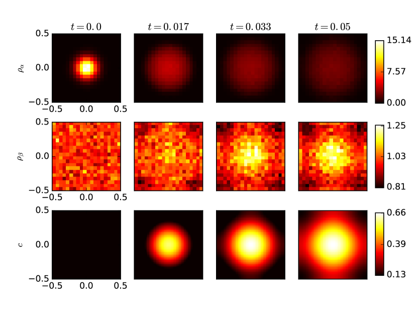
Figure 1: Visualisation of the simulation at times $t=0,T_{f}/3,2T_{f}/3$ and $t=T_{f}=0.05$, averaged over 2000 random realisations. (Top row) Histograms of the $\alpha$ particle density $\rho_{\alpha}$ normalised by $N_{\alpha}$. (Middle row) Histograms of the $\beta$ particle density $\rho_{\beta}$ normalised by $N_{\beta}$. (Bottom row) Chemical concentration $c$. Parameters used: $N_{\alpha}(0)=N_{\beta}(0)=100,\epsilon=0.02,r_{\alpha}=10,r_{\beta}=0,D_{\alpha}=0.1,D_{\beta}=1,D_{c}=1,k_{\alpha}=0.1,k_{\beta}=0.03,\Delta t=\frac{(0.23\epsilon)^{2}}{4D_{\beta}},N_{c}=52$.

Figure 2 shows the number of $\alpha$ and $\beta$ particles, as well as the total number of all particles. This shows the dominant conversion of $\beta$ particles to $\alpha$, as well as the conservation of $N_{\alpha}+N_{\beta}$ over time.

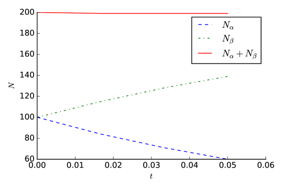
Figure 2: The evolution in time of the number of particles in each species, $N_{\alpha}$ and $N_{\beta}$, as well as the total number of particles $N_{\alpha}+N_{\beta}$. Results averaged over 2000 random realisations of the simulation.

Once we have the simulation framework established, we can begin conducting numerical experiments, altering the domain, parameters, initial distributions or behaviours of particles in order to explore different chemotactic behaviours, or taking advantage of the transparency of numerical simulation by measuring different quantities of interest. For example, in order to explore the average mean squared displacement for the $\alpha$ and $\beta$ particles we might wish to run another experiment using periodic boundary conditions, and track the total displacement of an individual particle from its initial position. We can do this by defining a new variable starting:

⬇

ABORIA_VARIABLE(starting, vdouble2, "starting_position");

and then initialising it to the starting position of each particle at the beginning of the simulation.

⬇

for (size_t i = 0; i < N; ++i) {

get<starting>(particles)[i] = get<position>(particles)[i];

}

Instead of the no-flux boundary conditions that we implemented previously (in Section 3.2), we will use periodic boundary conditions. Note that setting the periodic argument of init_neighbour_search to true (see Section 3.1) will cause particles that cross the periodic boundary to be automatically moved to the opposite boundary. We will counteract this by updating starting whenever a particle will cross the periodic boundary, so that the particle displacement thus far is preserved.

⬇

for (size_t d = 0; d < 2; ++d) {

if (get<next_position>(i)[d] < min[d]) {

get<starting>(i)[d] += L;

} else if (get<next_position>(i)[d] >= max[d]) {

get<starting>(i)[d] -= L;

}

}

Once we have our new variable in place we can simply calculate the mean squared displacement (MSD) of each particle by comparing its current position to the starting variable. We can use our Python wrapper to obtain both of these variables and calculate the MSD as a post-processing step.

Figure 3 shows the MSD for three different scenarios: (1) $N_{\alpha}=100,N_{\beta}=0$, (2) $N_{\alpha}=0,N_{\beta}=100$, and (3) $N_{\alpha}=50,N_{\beta}=50$. In all three the chemical gradient was set to be a constant by setting the chemical diffusion, production and consumption to zero ($D_{c}=0,k_{\alpha}=0,k_{\beta}=0$), and the initial profile equal to $c({\bf x})=x$. The chemical concentration does not satisfy the periodic boundary conditions in this case, however, its gradient is does and this is the only factor influencing the simulation via the drift term on the $\beta$ particles. The diffusion constant for each species was $D_{\alpha}=D_{\beta}=1$, and reactions between particles types are turned off. For simulation (1) the $\alpha$ particles are not affected by the drift term and so the MSD is a straight line with a low gradient. For simulation (2) the $\beta$ particles are affected by the constant drift, which adds a dominant $t^{2}$ term to their MSD. For simulation (3) the reactions are turned on again and there are both $\alpha$ and $\beta$ cells, so the net effect on the MSD is a combination of these two behaviours.

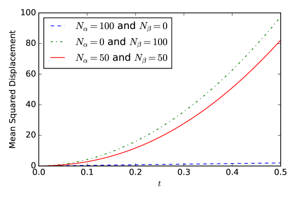
Figure 3: The Mean Squared Displacement (MSD) was calculated for three different simulations: (1) $N_{\alpha}=100,N_{\beta}=0$ with reactions off, (2) $N_{\alpha}=0,N_{\beta}=100$ with reactions off, (3) $N_{\alpha}=50,N_{\beta}=50$, with reactions on. In all cases the chemical concentration was set to $c({\bf x})=x$ to induce a constant drift term for the $\beta$ particles. The MSD for (1) is purely diffusion driven and shows the correct linear growth. The MSD for (2) and (3) is dominated by the drift term on the $\beta$ particles, which gives the $t^{2}$ growth.

5 Conclusions

Particle-based models for biological processes have become of widespread use in mathematical biology. These come in many forms, with particle motions described by discrete or continuum random walks, complex interactions between particles (including reactions, hard-core interactions, or interaction potentials), and interactions with the environment (such as chemotaxis or transport through crowded or heterogeneous domains). In some cases, one also requires to couple a particle-based model, describing for example individuals cells, with a PDE model to represent a continuum field (such as a chemical concentration). In addition, despite their apparent simplicity, particle-based models can be challenging to implement and simulate, as they tend to scale badly with the number of particles in the system (which can be large in many applications) and, due to stochasticity, often many realisations of the same simulation are required.

This diversity in particle-based models combined with the computational challenges in simulations, makes the implementation of particle-based models far from straightforward. In this paper we presented Aboria, a C++ library, designed to provide the flexibility required to implement particle-based models commonly used in mathematical biology, in a high performance and easy to use fashion.

We have demonstrated the usage of Aboria implementing a model for cell diffusion and chemotaxis with short-range interactions. The model has many of the features described above, namely, cells move according to biased Brownian motion, they interact with each other and with a chemical (that is modelled as a continuum), and there are reactions that change the number of particles. We have shown how Aboria can be used in combination with Python to produce outputs such as the cell densities, numbers, and the mean square displacement.

References

- Abraham et al (2015) Abraham MJ, Murtola T, Schulz R, Páll S, Smith JC, Hess B, Lindahl E (2015) Gromacs: High performance molecular simulations through multi-level parallelism from laptops to supercomputers. SoftwareX 1:19–25
- Andrews and Bray (2004) Andrews SS, Bray D (2004) Stochastic simulation of chemical reactions with spatial resolution and single molecule detail. Phys Biol 1(3):137–151
- Betzig et al (2006) Betzig E, Patterson GH, Sougrat R, Lindwasser OW, Olenych S, Bonifacino JS, Davidson MW, Lippincott-Schwartz J, Hess HF (2006) Imaging intracellular fluorescent proteins at nanometer resolution. Science 313(5793):1642–1645
- Bruna (2012) Bruna M (2012) Excluded-volume Effects in Stochastic Models of Diffusion. PhD thesis, University of Oxford
- Bruna and Chapman (2012) Bruna M, Chapman SJ (2012) Excluded-volume effects in the diffusion of hard spheres. Phys Rev E 85(1):011103
- Bruna et al (2017) Bruna M, Chapman SJ, Robinson M (2017) Diffusion of Particles with Short-Range Interactions. SIAM J Appl Math 77(6):2294–2316
- Dallon and Othmer (1997) Dallon JC, Othmer HG (1997) A discrete cell model with adaptive signalling for aggregation of Dictyostelium discoideum. Phil Trans R Soc B: Biol Sci 352(1351):391–417
- D’Orsogna et al (2006) D’Orsogna MR, Chuang Y, Bertozzi AL, Chayes LS (2006) Self-Propelled Particles with Soft-Core Interactions: Patterns, Stability, and Collapse. Phys Rev Lett 96(10):104302
- Eastman et al (2012) Eastman P, Friedrichs MS, Chodera JD, Radmer RJ, Bruns CM, Ku JP, Beauchamp KA, Lane TJ, Wang LP, Shukla D, et al (2012) Openmm 4: a reusable, extensible, hardware independent library for high performance molecular simulation. Journal of Chemical Theory and Computation 9(1):461–469
- Erban et al (2007) Erban R, Chapman J, Maini PK (2007) A practical guide to stochastic simulations of reaction-diffusion processes. arXiv 0704.1908
- Fong and Darve (2009) Fong W, Darve E (2009) The black-box fast multipole method. Journal of Computational Physics 228(23):8712–8725
- Franz and Erban (2013) Franz B, Erban R (2013) Hybrid Modelling of Individual Movement and Collective Behaviour. In: Dispersal, Individual Movement and Spatial Ecology, Springer, Berlin, Heidelberg, Berlin, Heidelberg, pp 129–157
- Franz et al (2013) Franz B, Xue C, Painter KJ, Erban R (2013) Travelling Waves in Hybrid Chemotaxis Models. Bull Math Biol 76(2):377–400
- Gillespie (1977) Gillespie DT (1977) Exact stochastic simulation of coupled chemical reactions. J Phys Chem 81(25):2340–2361
- Greengard and Rokhlin (1987) Greengard L, Rokhlin V (1987) A fast algorithm for particle simulations. Journal of computational physics 73(2):325–348
- Guo et al (2008) Guo Z, Sloot PMA, Tay JC (2008) A hybrid agent-based approach for modeling microbiological systems. J Theor Biol 255(2):163–175
- Hutzenthaler et al (2012) Hutzenthaler M, Jentzen A, Kloeden PE (2012) Strong convergence of an explicit numerical method for SDEs with nonglobally Lipschitz continuous coefficients. The Annals of Applied Probability 22(4):1611–1641
- Jeon et al (2010) Jeon J, Quaranta V, Cummings PT (2010) An Off-Lattice Hybrid Discrete-Continuum Model of Tumor Growth and Invasion. Biophys J 98(1):37–47
- McLennan et al (2012) McLennan R, Dyson L, Prather KW, Morrison JA, Baker RE, Maini PK, Kulesa PM (2012) Multiscale mechanisms of cell migration during development: theory and experiment. Development 139(16):2935–2944
- Middleton et al (2014) Middleton AM, Fleck C, Grima R (2014) A continuum approximation to an off-lattice individual-cell based model of cell migration and adhesion. J Theor Biol 359:220–232
- Newman and Grima (2004) Newman TJ, Grima R (2004) Many-body theory of chemotactic cell-cell interactions. Phys Rev E 70(5):051916
- Robinson and Bruna (2017) Robinson M, Bruna M (2017) Particle-based and meshless methods with Aboria. SoftwareX 6 IS -:172–178
- Scala et al (2007) Scala A, Voigtmann T, De Michele C (2007) Event-driven Brownian dynamics for hard spheres. J Chem Phys 126(13):134109
- Stroustrup (2013) Stroustrup B (2013) The C++ programming language. Pearson Education