Unified atmospheric neutrino passing fractions for large-scale neutrino telescopes

Abstract

The atmospheric neutrino passing fraction, or self-veto, is defined as the probability for an atmospheric neutrino not to be accompanied by a detectable muon from the same cosmic-ray air shower. Building upon previous work, we propose a redefinition of the passing fractions by unifying the treatment for muon and electron neutrinos. Several approximations have also been removed. This enables performing detailed estimations of the uncertainties in the passing fractions from several inputs: muon losses, cosmic-ray spectrum, hadronic-interaction models and atmosphere-density profiles. We also study the passing fractions under variations of the detector configuration: depth, surrounding medium and muon veto trigger probability. The calculation exhibits excellent agreement with passing fractions obtained from Monte Carlo simulations. Finally, we provide a general software framework to implement this veto technique for all large-scale neutrino observatories.

I Introduction

The detection of the first high-energy neutrinos of extraterrestrial origin Aartsen et al. (2013a) marked the beginning of neutrino astronomy. As we move from this first observation to precision physics using these astrophysical neutrino events, it becomes crucial to improve our understanding of atmospheric neutrinos, which together with atmospheric muons, represent the main backgrounds. Currently, the IceCube neutrino telescope has detected high-energy astrophysical neutrinos at a significance of $>6\sigma$ using high-energy starting events (HESE) Aartsen et al. (2013b, 2014, 2015a, 2017). This is further complemented by the observation of a compatible astrophysical flux using through-going muon neutrino events Aartsen et al. (2015b, 2016). Quantifying uncertainties on the atmospheric neutrino background becomes even more relevant for the medium energy starting event (MESE) sample Aartsen et al. (2015c), which extends to lower energies than the HESE sample. Recently, the ANTARES neutrino telescope has also carried out a search for the cosmic diffuse neutrino flux using nine years of up-going track- and shower-like events Albert et al. (2018). A small excess of high-energy events over the expected atmospheric background was identified, with a significance of $1.6\sigma$ and fully compatible with IceCube observations.

A major background in searches for astrophysical neutrinos comes from atmospheric muons. For this reason, neutrino telescopes primarily considered neutrinos coming from the direction passing through the Earth. The Earth is a very efficient shield of the high atmospheric muon flux, almost eliminating this background. This strategy, however, limits the solid angle of observation to half of the sky. Using also cascades Beacom and Candia (2004) and down-going events increases the statistics significantly. To use down-going neutrinos in astrophysical neutrino searches, an efficient method of vetoing atmospheric muons is required. Although ANTARES is too small to include an outer muon veto, larger detectors such as IceCube Achterberg et al. (2006) have used part of their instrumented volumes as active vetos for down-going muon, and KM3NeT Adrián-Martínez et al. (2016) and Baikal-GVD Avrorin et al. (2018) telescopes may. These muons are produced together with down-going atmospheric neutrinos and may reach the detector at the same time and from the same direction. A neutrino signal in coincidence with a passing muon could significantly reduce the expected atmospheric neutrino background. This idea was first applied by Schönert, Gaisser, Resconi, and Schulz (SGRS) Schönert et al. (2009) to the case of muons produced from the decay of the same parent as the muon neutrino. This was later extended for both electron and muon neutrinos by Gaisser, Jero, Karle, and van Santen (GJKvS) Gaisser et al. (2014), who considered muons produced from other parents in the same cosmic-ray shower.

Indeed, an outer layer veto is used by some IceCube analyses to significantly reduce the atmospheric muon and neutrino backgrounds. Atmospheric muons are rejected if they deposit enough light on the veto layer before entering the fiducial volume of the analysis. Atmospheric neutrinos are indirectly rejected if they are accompanied by muons, produced in the same air shower, that trigger the veto. These accompanying muons reduce the probability that neutrinos that pass the veto are of atmospheric origin. This is in fact what drives the bound on the atmospheric prompt neutrino contribution in HESE Aartsen et al. (2014) and MESE Aartsen et al. (2015c) analyses. At high energies, veto suppression in the Southern hemisphere turns out to be larger than that of Earth absorption in the Northern one (see Fig. 1), in contradiction with the observed zenith distribution. The previous works did not study the systematic uncertainties of these probabilities and used several simplifying approximations. The objective of this work is to present a more precise calculation that also allows for including systematic uncertainties and detector characteristics. To summarize, Fig. 1 shows the effect of the suppression of the atmospheric neutrino fluxes, as a function of the cosine of the zenith angle $\theta_{z}$, for two energies (left 10 TeV and right 100 TeV). Note that neutrino absorption in the Earth is also included for $\cos\theta_{z}<0$ using the $\nu$FATE code Vincent et al. (2017). The ratio of the passing to the total flux is called the passing fraction.

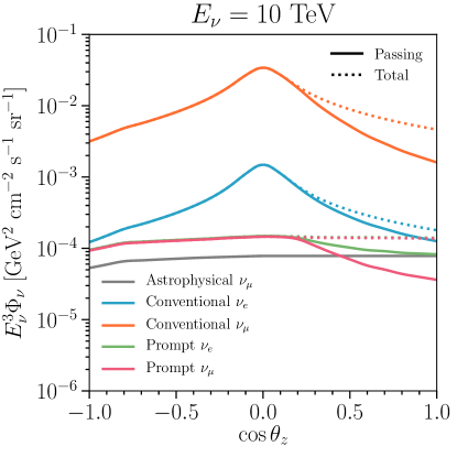
(a)

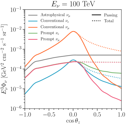
(b)

Figure 1: Atmospheric neutrino passing fluxes, as a function of the cosine of the zenith angle $\theta_{z}$. We compare passing fluxes after applying the rejection factor described in this work (solid) with the fluxes before entering the detector (dotted). The results are shown, from top to bottom in the left panel, for conventional $\nu_{\mu}$ (orange), conventional $\nu_{e}$ (blue), prompt $\nu_{e}$ (green) and prompt $\nu_{\mu}$ (magenta) fluxes. The astrophysical $\nu_{\mu}$ (gray) $E_{\nu}^{-2.19}$ flux Aartsen et al. (2017) lies beneath the others and is not subject to the atmospheric rejection factor. Note that absorption in the Earth is included for $\cos\theta_{z}<0$. Left panel: $E_{\nu}=10$ TeV. Right panel: $E_{\nu}=100$ TeV. Note the conventional $\nu_{e}$ flux drops below the other channels at $\cos\theta_{z}=-1$ while the astrophysical $\nu_{\mu}$ flux rises to just below the conventional $\nu_{\mu}$ channel.

The atmospheric neutrino passing fraction depends on the primary shower development and on the muon energy losses in the medium. This probability is conditional on the neutrino flavor, energy, zenith angle, and parent particle. In this work, we are especially concerned with uncertainties in the muon energy losses, the primary cosmic-ray spectrum, the hadronic-interaction model, and the atmosphere-density model. In order to study these uncertainties, we created a new framework that relies on the Matrix Cascade Equation (MCEQ) package Fedynitch (2017); Fedynitch et al. (2015, 2018). Naturally, our calculation is designed so that the primary cosmic-ray spectrum, the hadronic-interaction model, and the atmosphere-density model can be changed. In addition, we include accurate treatment of muon energy losses in different media and the possibility to tune the detector’s characterization: depth, medium, and veto’s response to incident muons. Moreover, to validate our calculation of the atmospheric neutrino passing fractions, we have compared our results with those obtained from a detailed simulation using the COsmic Ray SImulations for KAscade (CORSIKA) program Heck et al. (1998); Heck and Pierog (2018) and we find them in extremely good agreement.

The paper is organized as follows. Section II describes the main ingredients that enter our computation of the passing fractions. In section II.1 we discuss different inputs related to air shower development. In section II.2 we define the probability for a muon to reach the detector and trigger the veto at some depth below the surface. In section III, we build upon previous work Schönert et al. (2009); Gaisser et al. (2014) and define the passing fractions for atmospheric electron (section III.1), muon (section III.2), and tau (section III.3) neutrinos. We also evaluate the effect of previous approximations on the passing fraction and perform a direct comparison to those results in section III.4. Different sources of systematic uncertainty are discussed in section IV: muon energy losses in section IV.1, primary cosmic-ray spectrum in section IV.2, hadronic-interaction model in section IV.3, and atmosphere-density model in section IV.4. In section V, we illustrate the effects of changing parameters related to the detector configuration: the detector depth in section V.1, the surrounding medium in section V.2, and the veto’s response to passing muons in section V.3. Finally, in section VI we draw our final conclusions. In appendix A we briefly describe the publicly available code to calculate atmospheric neutrino passing fractions and in appendix B we provide, in tabulated form, passing fractions for our default settings.

II Cosmic-ray showers and penetrating muons

II.1 Shower physics

Interactions of cosmic rays with nuclei of the Earth’s atmosphere produce a flux secondary particles, which can eventually decay into muons and neutrinos that could reach detectors located at surface or underground. While the spectra of these atmospheric leptons peak around GeV energies, it extends to high energies with an approximate power-law dependence. The final lepton spectra at the Earth’s surface depend on the energy distribution and composition of the primary cosmic-ray flux, as well as on the properties of the hadronic interactions that control their production, on the density profile, and composition of the atmosphere. We use the open-source numerical code MCEQ Fedynitch (2017); Fedynitch et al. (2015, 2018) to compute the different distributions of all secondary particles, as a function of energy, direction, and slant depth. Moreover, for comparisons and tests of our computations, we also show the results from a dedicated full Monte Carlo simulation with CORSIKA Heck et al. (1998); Heck and Pierog (2018).

Except otherwise noted, our default model for the primary cosmic-ray spectrum is the three-population model from Gaisser Gaisser (2012) (H3a), that follows Hillas’s proposal Hillas (2006), with each population containing five groups of nuclei that cut off exponentially at a characteristic rigidity. This is the minimal assumption if the galactic-extragalactic transition occurs at the ankle. In section IV.2 we also consider other models for the primary cosmic-ray spectrum.

For the description of multiparticle production and extensive air shower development we use the recently released SIBYLL 2.3c Riehn et al. (2017) as our default hadronic-interaction model, which also includes charmed particles production. In section IV.3 we also compare the results obtained with other hadronic-interaction models.

To characterize the density profile of the atmosphere, we use the MSIS-90-E model at the South Pole corresponding to July 1, 1997 Labitzke et al. (1985); Hedin (1991), as our default model, location, and period of the year. We comment below on the uncertainties on the characterization of the Earth’s atmosphere, from model to model differences, from seasonal variations, and from different locations.

Given that the CORSIKA simulation uses SIBYLL 2.3 Riehn et al. (2015, 2016) as the hadronic-interaction model, instead of SIBYLL 2.3c, whenever we compare our results with those from the simulation, we also use SIBYLL 2.3. Our default cosmic-ray primary spectrum and atmosphere-density model are chosen to coincide used in the CORSIKA simulation.

Atmospheric neutrinos are typically categorized as conventional or prompt based on their parent particle Gaisser and Honda (2002). Conventional atmospheric muon neutrinos are defined to be those that come from pion or kaon decay Barr et al. (2004); Honda et al. (2007, 2011); Petrova et al. (2012); Sinegovskaya et al. (2015); Gaisser and Klein (2015); Honda et al. (2015). At energies above $\sim 100$ GeV the flux of conventional muon neutrinos transitions from predominantly those produced by pion decays to predominantly those produced by kaon decays. At those high energies, conventional electron neutrinos are produced almost entirely from kaon decays. In this work, conventional neutrinos are defined as those produced from the decays of $\pi^{\pm}$, $K^{\pm}$, $K^{0}_{L}$, $K^{0}_{s}$, and $\mu^{\pm}$. Prompt atmospheric neutrinos are produced from the decay of charmed and bottom hadrons, which have a very short lifetime and decay almost immediately after production Gondolo et al. (1996); Pasquali et al. (1999); Pasquali and Reno (1999); Martin et al. (2003); Enberg et al. (2008); Bhattacharya et al. (2015); Garzelli et al. (2015); Gauld et al. (2015, 2016); Bhattacharya et al. (2016); Garzelli et al. (2017); Benzke et al. (2017); Sinegovsky and Sorokovikov (2017). This is also the reason their flux follows a power-law with a spectral index one unit harder than the conventional one. This flux begins to dominate at around $100$ TeV and the dominant contributions come from $D^{\pm}$, $D^{0}$, $\bar{D}^{0}$, $\Lambda_{c}^{+}$, and $D_{s}^{\pm}$, with the last two components being less important Fedynitch et al. (2015). In this work, we consider prompt atmospheric neutrinos from the decays of charmed mesons, $D^{\pm}$, $D^{\pm}_{s}$, $D^{0}$, and $\bar{D}^{0}$. The dominant two-body decay channels are $\pi^{\pm}\rightarrow\mu^{\pm}+\overset{\scriptscriptstyle(-)}{\nu}_{\!\!\mu}$ ($99.99\%$) and $K^{\pm}\rightarrow\mu^{\pm}+\overset{\scriptscriptstyle(-)}{\nu}_{\!\!\mu}$ ($63.56\%$). Almost all other atmospheric neutrinos are produced via $n$-body processes. As described in section III.2, we include the $n$-body decay spectra, obtained using PYTHIA 8.1 Sjöstrand et al. (2008), of $K^{0}_{L}$ for conventional muon neutrinos and $D^{+}$, $D^{0}$, $D_{s}^{+}$, and their antiparticles for prompts.

II.2 Penetrating muons and vetos in underground detectors

The concept of the atmospheric neutrino passing fraction is based on the coincidence, in time and direction, between a neutrino event and a muon produced in the same cosmic-ray shower. Thus, one of the key ingredients in the calculation of the atmospheric neutrino passing fractions is ${\cal P}_{\rm reach}\left(E_{\mu}^{\rm f}\,|\,E_{\mu}^{\rm i},\,X_{\mu}\right)$, the probability for a muon, produced with energy $E_{\mu}^{\rm i}$ and traversing a slant depth $X_{\mu}$ (in g/cm²) in a particular medium, to reach the detector with energy $E_{\mu}^{\rm f}$. Given that the slant depth of the atmosphere is very small, muon energy losses before entering the Earth are negligible, so only the path inside the Earth before reaching the detector is relevant. This is fully determined by $\theta_{z}$, the zenith angle in detector’s coordinates of the incoming muon, whose direction is assumed to coincide with that of the neutrino. In Earth’s surface coordinates, $\sin^{2}\theta_{z}^{s}=\left(1-d_{\rm det}/R_{\oplus}\right)^{2}\,\sin^{2}\theta_{z}$, where $d_{\rm det}$ is the depth of the detector and $R_{\oplus}$ is the Earth’s radius.

In the original work where the passing fraction for atmospheric muon neutrinos was proposed Schönert et al. (2009), ${\cal P}_{\rm reach}$ was approximated by a Dirac delta function with the final muon energy $E_{\mu}^{\rm f}$ set by a simple average relation obtained from the Muon Monte Carlo (MMC) code Chirkin and Rhode (2004). Explicitly, ${\cal P}_{\rm reach}^{\rm SGRS}(E_{\mu}^{\rm f}\,|\,E_{\mu}^{\rm i},\,X_{\mu})=\delta\left(X_{\mu}-X_{\mu}^{\rm median}(E_{\mu}^{\rm i},E_{\mu}^{\rm f})\right)\left|dX_{\mu}^{\rm median}/dE_{\mu}^{\rm f}\right|$, where $X_{\mu}^{\rm median}(E_{\mu}^{\rm i},E_{\mu}^{\rm f})$ is the median slant depth a muon with initial energy $E_{\mu}^{\rm i}$ propagates so that its final energy is $E_{\mu}^{\rm f}$. In this work, we take into account fluctuations from stochastic losses of muons propagating through the Earth toward the detector, and build probability distribution functions for ${\cal P}_{\rm reach}$ using MMC Chirkin and Rhode (2004). The inclusion of stochastic losses results in shorter average propagation distances Lipari and Stanev (1991) than if only continuous losses are considered. Moreover, taking into account fluctuations is especially important when the tails of the survival probabilities are relevant for distances beyond the average range, and results in larger atmospheric neutrino passing fractions for more horizontal directions. Nevertheless, for more vertical trajectories, these tails become important for distances below the average range and tend to reduce the passing fractions. This is discussed in the next section.

Next, in order to account for the detector veto’s response to muons, we introduce ${\cal P}_{\rm light}(E_{\mu}^{\rm f})$, which is the probability for a muon entering the detector with energy $E_{\mu}^{\rm f}$ to light the veto. This probability is both detector and event selection dependent and should be explicitly calculated for each analysis. In this paper, following previous work, we study toy ${\cal P}_{\rm light}(E_{\mu}^{\rm f})$. With our notation, the approach followed in Refs. Schönert et al. (2009); Gaisser et al. (2014) implies that ${\cal P}_{\rm light}$ is equivalent to a step-like function above some muon energy threshold, $E_{\mu}^{\rm th}$, that is, ${\cal P}_{\rm light}^{\rm SGRS}(E_{\mu}^{\rm f})=\Theta\left(E_{\mu}^{\rm f}-E_{\mu}^{\rm th}\right)$. As in Ref. Gaisser et al. (2014), we consider as our default $E_{\mu}^{\rm th}=1$ TeV. Nevertheless, our implementation is completely general and allows one to use functions with a smooth transition around the nominal threshold energy. As an example, we also consider a sigmoid, defined as the cumulative distribution function of a Gaussian, ${\cal P}_{\rm light}(E_{\mu}^{\rm f})=\Phi\left(\left(E_{\mu}^{\rm f}-E_{\mu}^{\rm th}\right)/\sigma_{\mu}\right)$ with $E_{\mu}^{\rm th}=0.75$ TeV and $\sigma_{\mu}=0.25$ TeV. Note that this trigger probability applies individually to each muon that reaches the detector. To fully account for the different energies in bundles of muons produced in the shower, ${\cal P}_{\rm light}$ can be redefined to dependent on the muon multiplicities and the bundle energy distribution.

Once ${\cal P}_{\rm reach}$ is obtained and ${\cal P}_{\rm light}$ determine, what matters in practice is the fraction of muons that reach and trigger the detector’s veto, which we define as

$${\cal P}_{\rm det}\left(E_{\mu}^{\rm i},\,X_{\mu}(\theta_{z})\right)\equiv\int dE_{\mu}^{\rm f}\,{\cal P}_{\rm reach}\left(E_{\mu}^{\rm f}\,|\,E_{\mu}^{\rm i},\,X_{\mu}(\theta_{z})\right)\,{\cal P}_{\rm light}(E_{\mu}^{\rm f})~{}.$$ (1)

Note that losses also depend on the medium and not only on the slant depth, whose dependence on $\theta_{z}$ we write explicitly. If the medium surrounding the detector is homogeneous, $X_{\mu}$ can be exchanged by the distance without loss of generality. Also notice that, if the range is approximated by its median value (${\cal P}_{\rm reach}$ as a Dirac delta function), ${\cal P}_{\rm det}$ follows the same shape as ${\cal P}_{\rm light}$. If ${\cal P}_{\rm light}$ is taken to be a step-like function, it results in the ${\cal P}_{\rm det}$ effectively used in Refs. Schönert et al. (2009); Gaisser et al. (2014),

$${\cal P}_{\rm det}^{\rm SGRS}\left(E_{\mu}^{\rm i},\,X_{\mu}\right)=\int dE_{\mu}^{\rm f}\,{\cal P}_{\rm reach}^{\rm SGRS}(E_{\mu}^{\rm f}\,|\,E_{\mu}^{\rm i},\,X_{\mu})\,{\cal P}_{\rm light}^{\rm SGRS}(E_{\mu}^{\rm f})=\Theta\left(X_{\mu}^{\rm median}(E_{\mu}^{\rm i},E_{\mu}^{\rm th})-X_{\mu}\right)~{}.$$ (2)

For clarity, from now on we will use $\theta_{z}$ instead of $X_{\mu}$ and will assume ice as the medium muons traverse before reaching the detector.

(a)

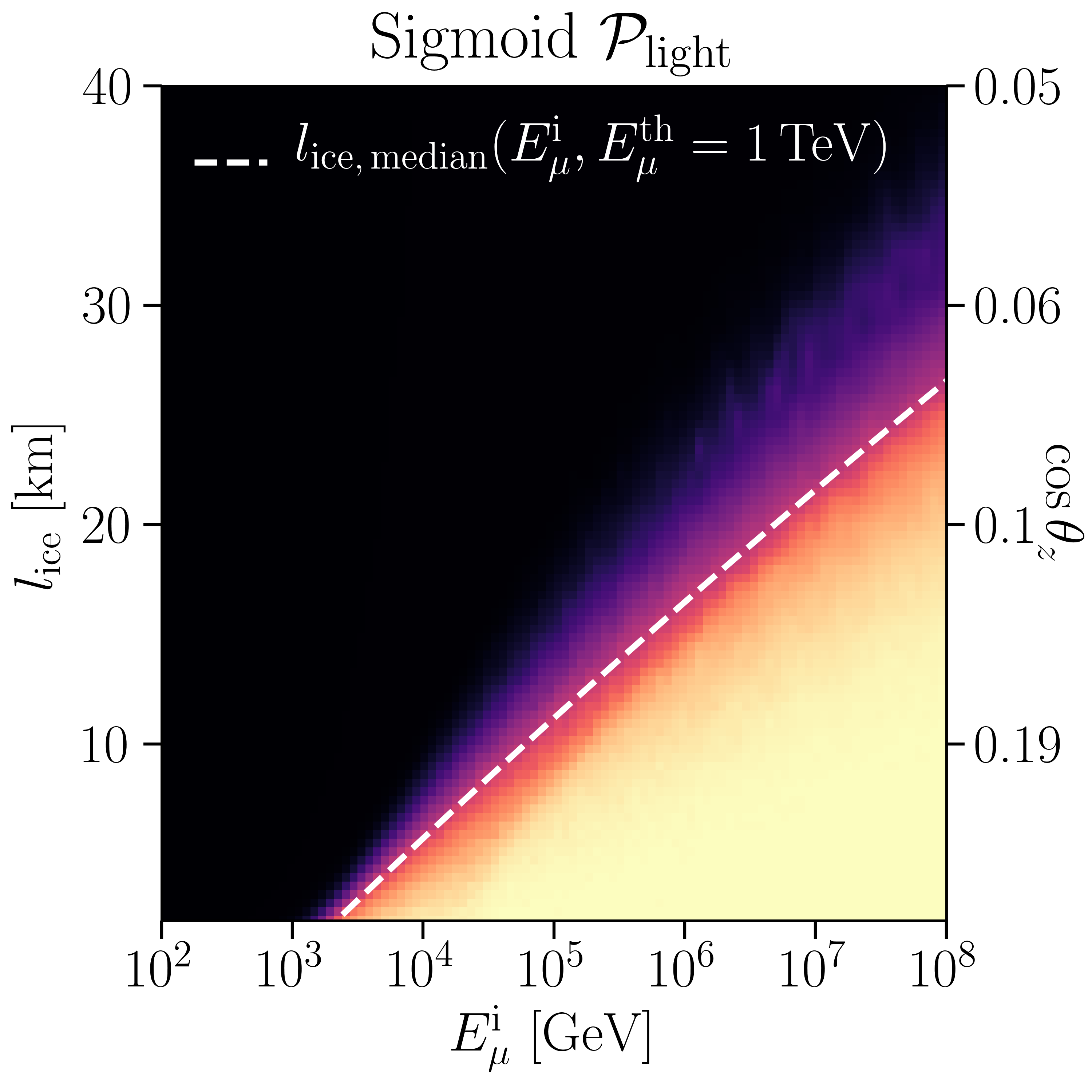
(b)

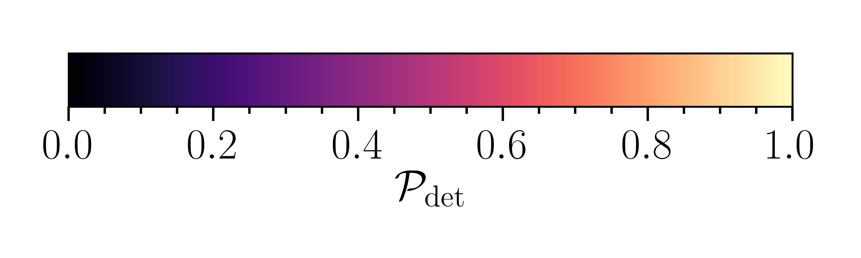
(c)

Figure 2: Fraction of muons that reach and trigger the detector’s veto, $\boldsymbol{{\cal P}_{\rm det}}$, as a function of the initial muon energy, $E_{\mu}^{\rm i}$, and the distance in ice, $l_{\rm ice}$. Also indicated is the equivalent $\cos\theta_{z}$ for a detector located at $d_{\rm det}=1.95$ km. We show ${\cal P}_{\rm det}$ using the muon range distribution (color) and the $E_{\mu}^{\rm i}$ required for the muon to survive a distance $l_{\rm ice}$ with at least $E_{\mu}^{\rm f}=1$ TeV 50% of the time (dashed), from Ref. Gaisser et al. (2014). Left panel: Heaviside trigger probability, ${\cal P}_{\rm light}(E_{\mu}^{\rm f})=\Theta(E_{\mu}^{\rm f}-E_{\mu}^{\rm th})$ with $E_{\mu}^{\rm th}=1$ TeV. Right panel: Sigmoid (defined as the cumulative distribution function of a Gaussian) trigger probability, ${\cal P}_{\rm light}(E_{\mu}^{\rm f})=\Phi\left(\left(E_{\mu}^{\rm f}-E_{\mu}^{\rm th}\right)/\sigma_{\mu}\right)$ with $E_{\mu}^{\rm th}=0.75$ TeV and $\sigma_{\mu}=0.25$ TeV. The minimum distance is $(l_{\rm ice})_{\rm min}=1.95$ km.

In Fig. 2 we show ${\cal P}_{\rm det}$ as a function of the initial muon energy, $E_{\mu}^{\rm i}$, and the distance from the Earth’s surface to the detector in ice, $l_{\rm ice}$. Also indicated is the equivalent $\cos\theta_{z}$ for a detector at depth $d_{\rm det}=1.95$ km, which we set as our default. The results are depicted for ${\cal P}_{\rm light}$ defined as a Heaviside function (left) or a sigmoid (right) and with the default setup in MMC to calculate ${\cal P}_{\rm reach}$ (see section IV.1). The darker regions indicate a lower probability and the lighter ones a higher probability of a muon to trigger the veto. In both panels, we also indicate the initial energy $E_{\mu}^{\rm i}$ required for the muon to survive a distance $l_{\rm ice}$ with at least $E_{\mu}^{\rm f}=1$ TeV 50% of the time (dashed), as computed in Ref. Gaisser et al. (2014); below that line ${\cal P}_{\rm det}^{\rm SGRS}=1$ and above ${\cal P}_{\rm det}^{\rm SGRS}=0$. In section V.1 we study the dependence of the passing fractions on the depth of the detector and in section V.2 on the medium surrounding the detector. The impact of different choices of ${\cal P}_{\rm light}$ are discussed in section V.3 and the effect of using the approximation with the median range, as compared to the complete treatment of muon energy losses, is studied in section III. As we will describe, the correct form of ${\cal P}_{\rm reach}$ introduces non-negligible corrections to the atmospheric neutrino passing fractions.

III Atmospheric neutrino passing fractions

The atmospheric neutrino passing fraction is the probability for an atmospheric neutrino not to be accompanied by a detectable muon from the same air shower. We denote this probability by ${\cal P}_{\rm pass}$ Schönert et al. (2009); Gaisser et al. (2014), which is defined as

$${\cal P}_{\rm pass}(E_{\nu},\theta_{z})=\frac{\phi_{\nu}^{\rm pass}(E_{\nu},\theta_{z})}{\phi_{\nu}(E_{\nu},\theta_{z})}~{},$$ (3)

where $E_{\nu}$ is the neutrino energy, $\phi_{\nu}(E_{\nu},\theta_{z})$ is the atmospheric neutrino differential flux, and $\phi_{\nu}^{\rm pass}(E_{\nu},\theta_{z})$ is the differential flux of atmospheric neutrinos that are not accompanied by a muon from the same shower that triggers the veto.

For reference, the atmospheric neutrino passing fractions obtained using our default settings are tabulated in Tables B. We define and discuss them below.

III.1 Passing fraction for electron neutrinos

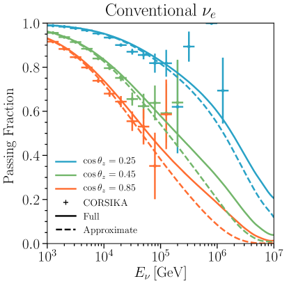
(a)

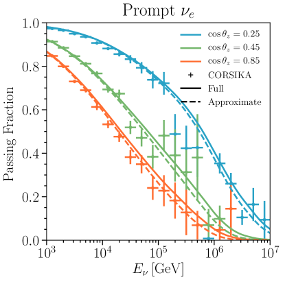
(b)

Figure 3: Passing fractions: effect of approximations on the energy of the shower giving rise to uncorrelated muons. Results are shown for three values of $\cos\theta_{z}$ (from top to bottom): 0.25 (blue), 0.45 (green), and 0.85 (orange); with the approach of this work (solid), Eq. (III.1), where the energy carried by the neutrino parent is subtracted from the rest of the shower which produces the muons to be triggered (i.e., $E_{\rm CR}-E_{p}$), and without this subtraction (dashed), Eq. (5), considering the cumulative muon yield from a shower with energy $E_{\rm CR}$. Results from the CORSIKA simulation are shown as crosses, with statistical error bars only. In all cases, the H3a primary cosmic-ray spectrum Gaisser (2012), the SIBYLL 2.3 hadronic-interaction model Riehn et al. (2015, 2016) and the MSIS-90-E atmosphere-density model at the South Pole on July 1, 1997 Labitzke et al. (1985); Hedin (1991) are used, and $d_{\rm det}=1.95$ km in ice and ${\cal P}_{\rm light}(E_{\mu}^{\rm f})=\Theta(E_{\mu}^{\rm f}-1\,{\rm TeV})$ are assumed. Left panel: Conventional $\nu_{e}$ passing fraction. Right panel: Prompt $\nu_{e}$ passing fraction.

Atmospheric electron neutrinos (antineutrinos) are created together with positrons (electrons) at the parent’s decay vertex and very rarely have a sibling muon. However, muons are produced in other branches of the shower. Following the approach of Ref. Gaisser et al. (2014), we define the passing fraction for electron neutrinos using the average properties of muons in a prototypical shower produced by an individual cosmic-ray nucleus $A$ with energy $E_{\rm CR}$. The atmospheric neutrino flux is given by,

$$\phi_{\nu}(E_{\nu},\theta_{z})=\sum_{A}\int dE_{\rm CR}\,\frac{dN_{A,\nu}}{dE_{\nu}}(E_{\rm CR},E_{\nu},\theta_{z})\,\phi_{A}(E_{\rm CR})~{},$$ (4)

where $\phi_{A}(E_{\rm CR})$ is the flux of primary cosmic-ray of nuclei $A$ and $dN_{A,\nu}/dE_{\nu}(E_{\rm CR},E_{\nu},\theta_{z})$ is the yield of neutrinos from a prototypical shower. The passing fraction can be obtained by weighting the total flux by the Poisson probability, ${\cal P}_{0\text{-}\mu}^{\rm shower}$, that no accompanying muon triggers the veto Gaisser et al. (2014),

$${\cal P}_{\rm pass}^{\rm uncor,GJKvS}(E_{\nu},\theta_{z})=\frac{1}{\phi_{\nu}(E_{\nu},\theta_{z})}\sum_{A}\int dE_{\rm CR}\,\frac{dN_{A,\nu}}{dE_{\nu}}(E_{\rm CR},E_{\nu},\theta_{z})\,\phi_{A}(E_{\rm CR})\,{\cal P}_{0\text{-}\mu}^{\rm shower}\left(N_{\mu}=0;\bar{N}_{A,\mu}^{\rm GJKvS}(E_{\rm CR},\theta_{z})\right)~{},$$ (5)

where

$${\cal P}_{0\text{-}\mu}^{\rm shower}\left(N_{\mu}=0;\bar{N}_{A,\mu}(E_{\rm CR},\theta_{z})\right)=e^{-\bar{N}_{A,\mu}(E_{\rm CR},\theta_{z})}~{},$$ (6)

and $\bar{N}_{A,\mu}(E_{\rm CR},\theta_{z})$ represents the expected number of muons in the prototypical shower that reach the detector and trigger the veto,

$$\bar{N}_{A,\mu}(E_{\rm CR},\theta_{z})=\int dE_{\mu}^{\rm i}\,\frac{dN_{A,\mu}}{dE_{\mu}^{\rm i}}(E_{\rm CR},E_{\mu}^{\rm i},\theta_{z})\,{\cal P}_{\rm det}\left(E_{\mu}^{\rm i},\theta_{z}\right)~{},$$ (7)

where $dN_{A,\mu}/dE_{\mu}^{\rm i}(E_{\rm CR},E_{\mu}^{\rm i})$ is the energy spectrum of muons with energy $E_{\mu}^{\rm i}$ from a prototypical shower with energy $E_{\rm CR}$ initiated from cosmic-ray nucleus $A$. If ${\cal P}_{\rm reach}$ is defined as a Dirac delta function following the dashed line in Fig. 2 and ${\cal P}_{\rm light}$ is taken as a Heaviside function with the threshold at $E_{\mu}^{\rm f}=1$ TeV, then this expression would correspond to the expected number of muons, $\bar{N}_{A,\mu}^{\rm GJKvS}$, as described in Ref. Gaisser et al. (2014).

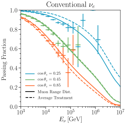
(a)

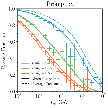
(b)

Figure 4: Passing fractions: effect of the treatment of muon losses in ice. Results are shown for three values of $\cos\theta_{z}$ (from top to bottom): 0.25 (blue), 0.45 (green), and 0.85 (orange); using the full muon range distribution (solid) or the median muon range (dashed), see Fig. 2. Results from the CORSIKA simulation are shown as crosses, with statistical error bars only. In all cases, the H3a primary cosmic-ray spectrum Gaisser (2012), the SIBYLL 2.3 hadronic-interaction model Riehn et al. (2015, 2016) and the MSIS-90-E atmosphere-density model at the South Pole on July 1, 1997 Labitzke et al. (1985); Hedin (1991) are used, and $d_{\rm det}=1.95$ km in ice and ${\cal P}_{\rm light}(E_{\mu}^{\rm f})=\Theta(E_{\mu}^{\rm f}-1\,{\rm TeV})$ are assumed. Left panel: Conventional $\nu_{e}$ passing fraction. Right panel: Prompt $\nu_{e}$ passing fraction.

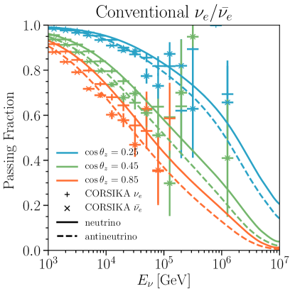
(a)

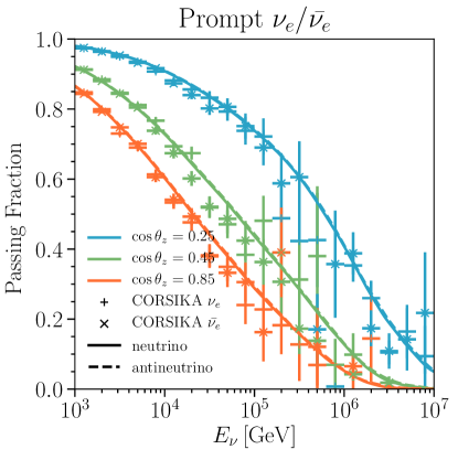
(b)

Figure 5: Passing fractions: neutrinos versus antineutrinos. Results are shown for three values of $\cos\theta_{z}$ (from top to bottom): 0.25 (blue), 0.45 (green), and 0.85 (orange); for neutrinos (solid) and antineutrinos (dashed). Results from the CORSIKA simulation for neutrinos ($+$) and antineutrinos ($\times$) are also shown, with statistical error bars only. In all cases, the H3a primary cosmic-ray spectrum Gaisser (2012), the SIBYLL 2.3 hadronic-interaction model Riehn et al. (2015, 2016) and the MSIS-90-E atmosphere-density model at the South Pole on July 1, 1997 Labitzke et al. (1985); Hedin (1991) are used, and $d_{\rm det}=1.95$ km in ice and ${\cal P}_{\rm light}(E_{\mu}^{\rm f})=\Theta(E_{\mu}^{\rm f}-1\,{\rm TeV})$ are assumed. Left panel: Conventional $\nu_{e}$ passing fraction. Right panel: Prompt $\nu_{e}$ passing fraction. Note that for prompts there are not differences between $\nu_{e}$ and $\bar{\nu}_{e}$.

As already recognized in Ref. Gaisser et al. (2014), in Eq. (7) the actual energy of the shower producing the uncorrelated muons is overestimated. This is because the energy of the parent particle that produces the observed neutrino must be subtracted. If the parent particle $p$ that creates the observed neutrino has energy $E_{p}$, the remaining energy is $E_{\rm CR}-E_{p}$. Therefore, we have to expand the neutrino yield in Eq. (5), from a cosmic-ray shower initiated by nucleus $A$, in terms of the yields from the different parent particles in the shower,

$$\frac{dN_{A,\nu}}{dE_{\nu}}(E_{\rm CR},E_{\nu},\theta_{z})=\int dE_{p}\,\int\frac{dX}{\lambda_{p}(E_{p},X)}\,\frac{dN_{p,\nu}}{dE_{\nu}}(E_{p},E_{\nu})\,\frac{dN_{A,p}}{dE_{p}}(E_{\rm CR},E_{p},X)~{},$$ (8)

where $dX/\lambda_{p}(E_{p},X)$ is the probability of a parent $p$ with energy $E_{p}$ to decay between slant depth $X$ and $X+dX$, and $\lambda_{p}(E_{p},X)=\rho(X)\,\tau_{p}\,E_{p}/m_{p}$ is the density, $\rho(X)$, times the decay length of parent particle $p$ with lifetime $\tau_{p}$, energy $E_{p}$, and mass $m_{p}$. The spectrum of neutrinos with energy $E_{\nu}$ from the decay of a parent particle $p$ with energy $E_{p}$ is given by $dN_{p,\nu}/dE_{\nu}(E_{p},E_{\nu})$. The spectrum of the parent particle $p$ at slant depth $X$, produced by a prototypical shower of energy $E_{\rm CR}$, initiated from cosmic-ray nucleus $A$ is given by $dN_{A,p}/dE_{p}(E_{\rm CR},E_{p},X)$.

In this way, the passing fraction for atmospheric electron neutrinos and antineutrinos can be rewritten,

$${\cal P}_{\rm pass}^{\rm uncor}(E_{\nu},\theta_{z}) =\frac{1}{\phi_{\nu}(E_{\nu},\theta_{z})}\,\sum_{A}\sum_{p}\int dE_{p}\int\frac{dX}{\lambda_{p}(E_{p},X)}\int dE_{\rm CR}$$

$$\frac{dN_{p,\nu}}{dE_{\nu}}(E_{p},E_{\nu})\,\frac{dN_{A,p}}{dE_{p}}(E_{\rm CR},E_{p},X)\,\phi_{A}(E_{\rm CR})\,{\cal P}_{0\text{-}\mu}^{\rm shower}\left(N_{\mu}=0;\bar{N}_{A,\mu}(E_{\rm CR}-E_{p},\theta_{z})\right)~{}.$$ (9)

If ${\cal P}_{0\text{-}\mu}^{\rm shower}=1$, then ${\cal P}_{\rm pass}^{\rm uncor}=1$ by construction. Note that we have explicitly subtracted $E_{p}$ from the energy $E_{\rm CR}$ of the cosmic-ray nuclei $A$ that generates the shower. This effect is shown in Fig. 3. The passing fractions for the conventional (left) and prompt (right) atmospheric $\nu_{e}$ flux are depicted for three different zenith angles, with (solid) and without (dashed) the $E_{p}$ subtraction in Eq. (III.1). We also show the results obtained from a dedicated Monte Carlo simulation with CORSIKA Heck et al. (1998); Heck and Pierog (2018) (crosses). The agreement with our results is excellent and we stress that there is no fit involved in our computations.

The approximate calculation without $E_{p}$ subtraction (dashed) slightly under-predicts the passing fractions. This is because $\bar{N}_{A,\mu}(E_{\rm CR},\theta_{z})>\bar{N}_{A,\mu}(E_{\rm CR}-E_{p},\theta_{z})$. The absolute difference is less than $0.05$ below $10^{5}$ TeV for conventional neutrinos and for all energies for prompt neutrinos. For energies above $10^{5}$ TeV the differences for conventional neutrinos can be more important, in particular for more vertical directions for which the passing fractions are smaller.

Once we have Eq. (III.1), we can evaluate the impact of ${\cal P}_{\rm reach}$, as described in the previous section. In Fig. 4, we illustrate the effect of taking the median muon range (dashed) instead of the full muon range distribution (solid). Both for the conventional (left) and the prompt (right) atmospheric $\nu_{e}$ fluxes, the median approximation overestimates the passing fraction for horizontal trajectories (right-blue), but underestimates it for more vertical directions (left-orange). This is also apparent from results presented in Ref. Gaisser et al. (2014) and it can be understood from Fig. 2. For small $\cos\theta_{z}$ muons have to traverse a larger portion of ice before reaching the detector. For propagation distances above $\sim 5$ km ($\cos\theta_{z}\lesssim 0.4$) with the Heaviside ${\cal P}_{\rm light}$, muons with lower $E_{\mu}^{\rm i}$ than that defining the median muon range have a small, but non-negligible, probability to trigger the veto. Thus, fewer muons reach the detector in the approximate case and consequently, the passing fractions are larger. On the contrary, for more vertical events, muons with lower $E_{\mu}^{\rm i}$ have a negligible probability to trigger the veto. This probability approaches one at higher $E_{\mu}^{\rm i}$, but not as sharply as the median approximation. Thus, when integrated, muons are more likely to trigger the veto in the approximate case and consequently, the passing fractions are smaller.

So far we have only shown results for $\nu_{e}$, but the passing fractions for the conventional $\bar{\nu}_{e}$ flux are different. In Fig. 5 we illustrate the differences between $\nu_{e}$ and $\bar{\nu}_{e}$ for the same angles considered in previous figures, along with results from the CORSIKA simulation. Again, the agreement between the simulation and our modeling is excellent for antineutrinos. The conventional $\bar{\nu}_{e}$ passing fractions are lower than those of conventional $\nu_{e}$. This is due to positively charged mesons being preferentially produced, leading to a harder spectrum than the negatively charged ones. For the prompt flux, the passing fractions are almost identical as they are mainly produced from gluon fusion Argüelles, C. A. and Halzen, F. and Wille, L. and Kroll, M. and Reno, M. H. (2015).

III.2 Passing fraction for muon neutrinos

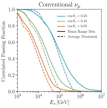
(a)

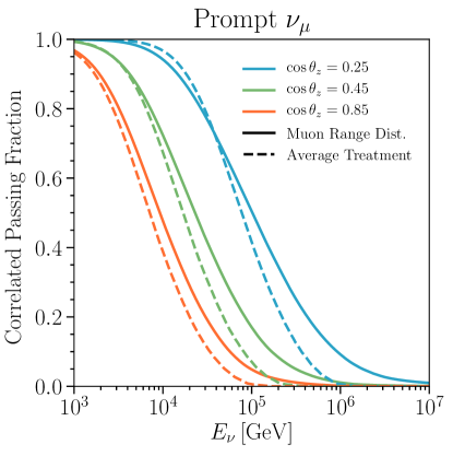
(b)

Figure 6: Correlated passing fractions: effect of the treatment of muon losses in ice. Same as Fig. 4 but only for the correlated part of the passing fraction for $\nu_{\mu}$.

Atmospheric muon neutrinos (and antineutrinos) from hadron decays are always produced alongside a muon. Therefore, the passing fraction of atmospheric muon neutrinos has a correlated suppression factor in addition to the uncorrelated one, described in the previous section. This extra suppression depends entirely on the probability of the sibling muon to trigger the veto, which in turn depends on the energy and incoming direction of the muon Schönert et al. (2009). For two-body decays, as in the case of pions and most kaons, the muon energy is $E_{\mu}^{\rm i}=E_{p}-E_{\nu}$, conditional on the muon neutrino energy $E_{\nu}$ from the decay of a parent particle $p$ with energy $E_{p}$. Thus, the energy spectrum of these muons is $dN_{p,\mu}^{2\text{-body}}/dE_{\mu}^{\rm i}(E_{p},E_{\nu},E_{\mu}^{\rm i})=\delta(E_{p}-E_{\nu}+E_{\mu}^{\rm i})$. For more generic $n$-body decays, as in the case of charmed hadrons, the probability of non-detection can be written as

$${\cal P}_{0\text{-}\mu}^{\rm sib}\left(\theta_{z}|E_{p},E_{\nu}\right)=1-\int dE_{\mu}^{\rm i}\,{\cal P}_{\rm det}\left(E_{\mu}^{\rm i},\theta_{z}\right)\frac{dN_{p,\mu}}{dE_{\mu}^{\rm i}}(E_{p},E_{\nu},E_{\mu}^{\rm i})~{}.$$ (10)

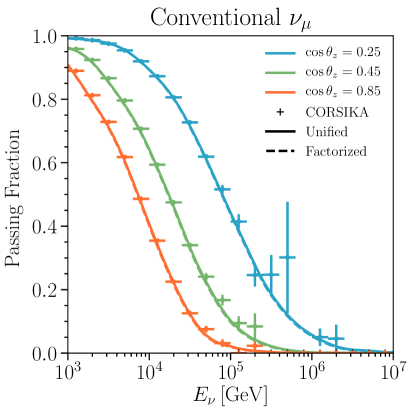
(a)

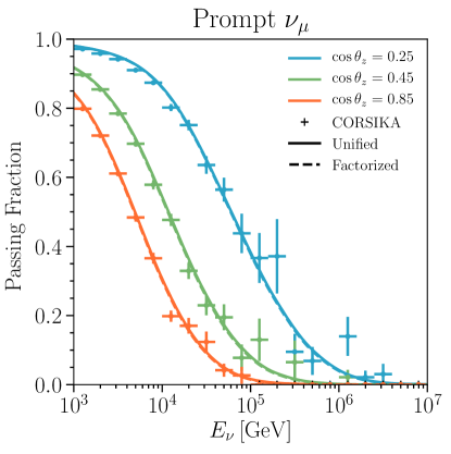
(b)

Figure 7: Passing fractions: differences between the unified and the factorized treatments for $\boldsymbol{\nu_{\mu}}$. Same as Fig. 3 regarding the approximations on the energy of the shower which gives rise to uncorrelated muons. Comparison of the unified treatment (solid), Eq. (III.2), and the approximate treatment (dashed), Eq. (15), which factorizes the correlated and uncorrelated passing fractions. The result is driven by the correlated part.

Now, it is necessary to express the neutrino flux in terms of the parent fluxes and their decays. As described in Sec. III.1, the decay probability of a parent $p$ at slant depth $X$ is $dX/\lambda_{p}(E_{p},X)$. Then, the differential flux of parent particles at slant depth $X$, $\phi_{A,p}(E_{p},X)$, can be defined in terms of the spectrum of parent particles with energy $E_{p}$ from a prototypical cosmic-ray shower, initiated from nucleus $A$, with energy $E_{\rm CR}$ and differential flux $\phi_{A}(E_{\rm CR})$, as

$$\phi_{A,p}(E_{p},X)=\int dE_{\rm CR}\,\frac{dN_{A,p}}{dE_{p}}(E_{\rm CR},E_{p},X)\,\phi_{\rm CR}(E_{\rm CR})~{}.$$ (11)

If we now express the energy spectrum of neutrinos with energy $E_{\nu}$ from the decay of a parent particle $p$ as $dN_{p,\nu}/dE_{\nu}(E_{p},E_{\nu})$, then the differential flux of atmospheric neutrinos at the surface of the Earth, $\phi_{\nu}(E_{\nu},\theta_{z})$, is given by

$$\phi_{\nu}(E_{\nu},\theta_{z})=\sum_{A}\sum_{p}\int dE_{p}\int\frac{dX}{\lambda_{p}(E_{p},X)}\,\frac{dN_{p,\nu}}{dE_{\nu}}(E_{p},E_{\nu})\,\phi_{A,p}(E_{p},X),$$ (12)

and therefore, we can define the correlated passing fraction as

$${\cal P}_{\rm pass}^{\rm cor}(E_{\nu},\theta_{z})=\frac{1}{\phi_{\nu}(E_{\nu},\theta_{z})}\,\sum_{A}\sum_{p}\int dE_{p}\int\frac{dX}{\lambda_{p}(E_{p},X)}\,\frac{dN_{p,\nu}}{dE_{\nu}}(E_{p},E_{\nu})\,\phi_{A,p}(E_{p},X)\,{\cal P}_{0\text{-}\mu}^{\rm sib}\left(\theta_{z}|E_{p},E_{\nu}\right).$$ (13)

In analogy with Fig. 4, Fig. 6 shows the effect of the correct treatment of the muon range distribution on the correlated passing fraction defined in Eq. (13). As described in section II.2, accounting for the stochasticity of muon energy losses smears the ${\cal P}_{\rm det}$ distribution from a Heaviside function, such that muons with lower $E_{\mu}^{\rm i}$ may be vetoed and muons with higher $E_{\mu}^{\rm i}$ may not be so. This effect is seen in the passing fraction, which drops at lower energies due to the increased vetoing probability of lower $E_{\mu}^{\rm i}$ muons and increases at higher energies due to the decreased vetoing probability of higher $E_{\mu}^{\rm i}$ muons. The transition energy is higher for more horizontal trajectories and in the relevant energy range, for more vertical trajectories, the effect is a general suppression of the passing fraction. Note also that in the case of a Heaviside $P_{\rm det}$, there is a shoulder due to the different contribution of pions and kaons to the neutrino flux. This gets smeared out when taking the muon range distribution into account.

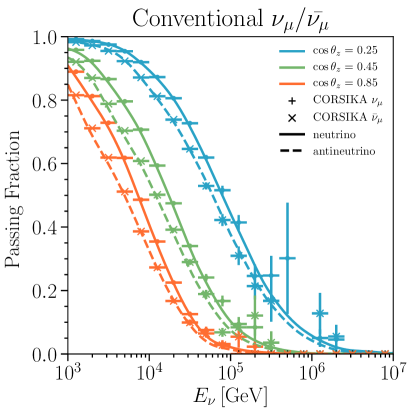
(a)

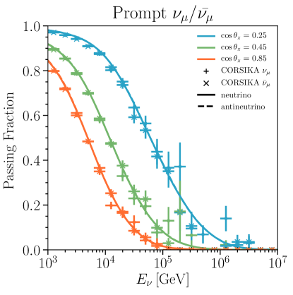
(b)

Figure 8: Passing fractions: neutrinos versus antineutrinos. Same as Fig. 5 but for $\nu_{\mu}$ and $\bar{\nu}_{\mu}$. Note that for prompt neutrinos there are not differences between $\nu_{\mu}$ and $\bar{\nu}_{\mu}$.

As discussed above, for two-body decays $E_{\mu}^{\rm i}=E_{p}-E_{\nu}$ and assuming Eq. (2) for the muon detection probability, Eq. (13) simplifies to

$${\cal P}_{\rm pass}^{\rm cor,SGRS}(E_{\nu},\theta_{z})=\frac{1}{\phi_{\nu}(E_{\nu},\theta_{z})}\,\sum_{A}\sum_{p}\int dE_{p}\int\frac{dX}{\lambda_{p}(E_{p},X)}\,\frac{dN_{p,\nu}}{dE_{\nu}}(E_{p},E_{\nu})\,\phi_{A,p}(E_{p},X)\,\left[1-{\cal P}_{\rm det}^{\rm SGRS}\left(E_{p}-E_{\nu},\theta_{z}\right)\right]~{}.$$ (14)

In this way, an approximate passing probability for muon neutrinos was defined as Gaisser et al. (2014)

$${\cal P}_{\rm pass}^{\rm GJKvS}(E_{\nu},\theta_{z})\equiv{\cal P}_{\rm pass}^{\rm cor,SGRS}(E_{\nu},\theta_{z})\,{\cal P}_{\rm pass}^{\rm uncor,GJKvS}(E_{\nu},\theta_{z})~{},$$ (15)

where we have used Eqs. (5) and (14).

However, the two-body approximation is not appropriate for the calculation of the passing fractions for the prompt fluxes, as neutrinos (and antineutrinos) come mainly from $D^{\pm}$, $D^{0}$, $\bar{D}^{0}$, $\Lambda_{c}^{+}$, and $D_{s}^{\pm}$ decays Fedynitch et al. (2015). A correct treatment of $n$-body decays requires evaluating the muon distributions from the decays of these particles and using Eq. (10). In this work, $dN_{p,\mu}/dE_{\mu}^{\rm i}$ was generated for $K^{0}_{L}$, $D^{+}$, $D^{0}$, and $D^{+}_{s}$.

The “factorized” approach in Eq. (15) can be further improved by combining Eqs. (III.1) and (13), which accounts for the correction in the energy of the prototypical shower, $E_{\rm CR}-E_{p}$. The new passing fraction can be defined as

$${\cal P}_{\rm pass}(E_{\nu},\theta_{z})=\frac{1}{\phi_{\nu}(E_{\nu},\theta_{z})}\,\sum_{A}\sum_{p} \int dE_{p}\int\frac{dX}{\lambda_{p}(E_{p},X)}\int dE_{\rm CR}\,\frac{dN_{p,\nu}}{dE_{\nu}}(E_{p},E_{\nu})\,\frac{dN_{A,p}}{dE_{p}}(E_{\rm CR},E_{p},X)\,\phi_{A}(E_{\rm CR})$$

$$\times{\cal P}_{0\text{-}\mu}^{\rm sib}\left(\theta_{z}|E_{p},E_{\nu}\right)\,{\cal P}_{0\text{-}\mu}^{\rm shower}\left(N_{\mu}=0;\bar{N}_{\mu,A}(E_{\rm CR}-E_{p},\theta_{z})\right),$$ (16)

where we have substituted Eq. (11) into Eq. (13). The numerator in this equation defines $\phi_{\nu}^{\rm pass}(E_{\nu},\theta_{z})$. In this way, Eq. (III.2) represents our master equation to obtain the passing fractions for atmospheric neutrinos. It can be applied directly to the case of electron neutrinos where no sibling muons are produced and thus, ${\cal P}_{0\text{-}\mu}^{\rm sib}\left(\theta_{z}|E_{p},E_{\nu}\right)=1$. In that case, Eq. (III.2) reduces to Eq. (III.1). More explicitly, we can substitute Eqs. (1), (6), and (10) to get

$${\cal P}_{\rm pass}(E_{\nu},\theta_{z})= \frac{1}{\phi_{\nu}(E_{\nu},\theta_{z})}\,\sum_{A}\sum_{p}\int dE_{p}\int\frac{dX}{\lambda_{p}(E_{p},X)}\int dE_{\rm CR}\,\frac{dN_{p,\nu}}{dE_{\nu}}(E_{p},E_{\nu})\,\frac{dN_{A,p}}{dE_{p}}(E_{\rm CR},E_{p},X)\,\phi_{A}(E_{\rm CR})$$

$$\times\left[1-\int\,dE_{\mu}^{\rm i}\,\frac{dN_{p,\mu}}{dE_{\mu}^{\rm i}}(E_{p},E_{\nu},E_{\mu}^{\rm i})\,\int dE_{\mu}^{\rm f}\,{\cal P}_{\rm light}(E_{\mu}^{\rm f})\,{\cal P}_{\rm reach}\left(E_{\mu}^{\rm f}|E_{\mu}^{\rm i},\theta_{z}\right)\right]\,e^{-N_{A,\mu}(E_{\rm CR}-E_{p},\theta_{z})}~{},$$ (17)

A comparison between the results for muon neutrinos obtained using Eq. (15) (factorizing the correlated and uncorrelated passing fractions) and those obtained with the more accurate Eq. (III.2), or equivalently Eq. (III.2), is shown in Fig. 7. The effect of the subtraction of $E_{p}$ from $E_{\rm CR}$ is smaller than in the case of electron neutrinos, shown in Fig. 3, due to ${\cal P}_{0\text{-}\mu}^{\rm sib}$ being a much more dominant factor than ${\cal P}_{0\text{-}\mu}^{\rm shower}$. Note that, for the uncorrelated part of the passing fraction, this subtraction is more important at higher energies, for which the correlated part is very small. Thus, the relative effect on the muon neutrino passing fraction is much smaller. Finally, comparisons of the passing fractions calculated for muon neutrinos and muon antineutrinos are shown in Fig. 8 and exhibit very good agreement with the Monte Carlo results, as in the case of electron neutrinos (Fig. 5).

III.3 Passing fraction for tau neutrinos

For down-going neutrinos at energies above $\sim$ TeV, the major atmospheric $\nu_{\tau}$ component is the prompt flux from $D_{s}$ decays into $\nu_{\tau}$ and $\tau$ and subsequent $\tau$ decays Pasquali and Reno (1999). The additional bottom-quark ($B^{+}$ and $B^{0}$) contribution represents a $\lesssim 10\%$ correction Pasquali and Reno (1999); Bhattacharya et al. (2016). The calculation of the uncorrelated passing fraction is still given by Eq. (III.1). However, the calculation of the correlated passing fraction is different from the conventional $\nu_{\mu}$ calculation. Conventional $\nu_{\mu}$ are produced mainly via two-body decays where $E_{\mu}^{\rm i}=E_{p}-E_{\nu}$. Prompt $\nu_{\tau}$, on the other hand, are more similar to to prompt $\nu_{\mu}$ in which correlated muons are produced from $n$-body decay. These muon decay distributions must be evaluated in order to calculate the $\nu_{\tau}$ passing fraction. At $\sim$ TeV energies, $\tau$ leptons are produced high in the atmosphere and can be assumed to decay without energy losses. Although Eq. (13) applies, ${\cal P}_{0\text{-}\mu}^{\rm sib}$ has to be specifically computed. In addition, there is a subleading contribution from the oscillated atmospheric $\nu_{\mu}$ flux Martin et al. (2003); Bulmahn and Reno (2010). The passing fraction for oscillated $\nu_{\tau}$ is identical to that for $\nu_{\mu}$, though the event signature would be different in the detector. There is another, $4-6$ orders of magnitude more subleading contribution due to tau pair production from muon losses in the atmosphere Bulmahn and Reno (2010). In this case, there is a correlated muon accompanying the $\nu_{\tau}$ from tau decays and the always present uncorrelated part.

At the relevant energies in this work, the atmospheric $\nu_{\tau}$ flux is about an order of magnitude smaller than the prompt $\nu_{e}$ and $\nu_{\mu}$ fluxes. Given our current knowledge of the atmospheric prompt flux, for which only upper bounds exist, and given the subleading nature of the $\nu_{\tau}$ component, we do not compute $\nu_{\tau}$ passing fractions and do not discuss this flux any further.

III.4 Improvements with respect to previous calculations

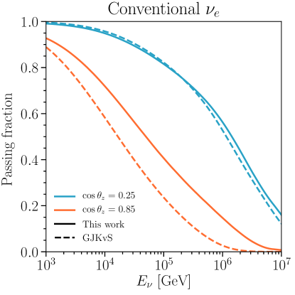
(a)

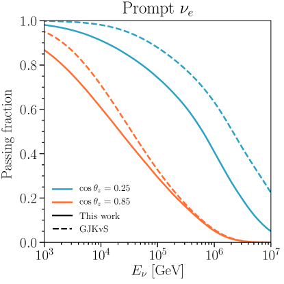
(b)

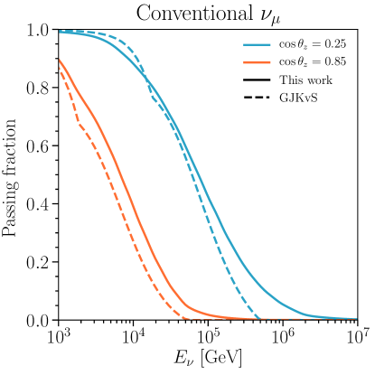
(c)

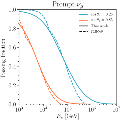
(d)

Figure 9: Passing fractions: comparison with previous work. Results are shown for two values of $\cos\theta_{z}=$ (from top to bottom): 0.25 (blue) and 0.85 (orange); with the calculation in this work (solid) and with that in Ref. Gaisser et al. (2014) (dashed). Our results are obtained with the H3a primary cosmic-ray spectrum Gaisser (2012), the SIBYLL 2.3c hadronic-interaction model Riehn et al. (2017), the MSIS-90-E atmosphere-density model at the South Pole on July 1, 1997 Labitzke et al. (1985); Hedin (1991), and assuming $d_{\rm det}=1.95$ km in ice and ${\cal P}_{\rm light}(E_{\mu}^{\rm f})=\Theta(E_{\mu}^{\rm f}-1\,{\rm TeV})$. They include all of the effects discussed in previous sections, Eq. (III.2). Top-left panel: Conventional $\nu_{e}$ passing fraction. Top-right panel: Prompt $\nu_{e}$ passing fraction. Bottom-left panel: Conventional $\nu_{\mu}$ passing fraction. Bottom-right panel: Prompt $\nu_{\mu}$ passing fraction.

The first proposal to calculate the suppression of the down-going atmospheric neutrino flux for high-energy neutrino telescopes only accounted for accompanying muons produced from the same decaying parent meson Schönert et al. (2009). Therefore, it was only applied to atmospheric muon neutrinos. The calculation was based on a several analytical approximations, applicable to neutrinos from pion and kaon decays and assuming a power-law primary cosmic-ray spectrum. As described above, the treatment of energy losses did not account for muon range distributions, and the criteria for muons to trigger the veto was a Heaviside function at some threshold energy. This allowed the final passing fractions to be expressed analytically.

The analytic treatment was generalized by including muons from other branches of the shower in which the neutrino was produced Gaisser et al. (2014), as explained in section III.1. This allowed part of the flux of down-going, atmospheric electron neutrinos to be excluded from the sample. This method used analytic approximations to describe the average properties of muons generated by cosmic rays for both conventional and prompt neutrino fluxes. These approximations were shown to correctly describe the results of the CORSIKA simulation. Indeed, $\bar{N}_{A,\mu}(E_{\rm CR},\theta_{z})$ was calculated by fitting a parameterized yield function to the CORSIKA simulation, which used the SIBYLL 2.1 Ahn et al. (2009) hadronic-interaction model for conventional atmospheric neutrinos and DPMJET-2.55 Ranft (1999a, b); Berghaus et al. (2008) for prompt atmospheric neutrinos. Along with the results from Ref. Schönert et al. (2009), this extra contribution led to Eq. (15). By not subtracting $E_{p}$ from $E_{\rm CR}$, the passing fraction for muon neutrinos accounted for the correlated muon more than once. In the case of the passing fraction for electron neutrinos, it led to the overestimation of the energy of the shower producing detectable muons. This allowed the correlated and uncorrelated rates to be factorized.

Our approach includes the parent spectra from cosmic-ray interactions in the atmosphere and led to the more accurate Eq. (III.2). It is a fully consistent definition of the passing fraction for both electron and muon neutrinos, as described in section III. In our treatment we also account, in full detail, for the stochasticity of muon energy losses by computing the muon range distributions. We stress that our approach also allows considering different detector configurations (depth, type of medium, muon vetoing efficiency), cosmic-ray primary spectra, hadronic-interaction models and atmosphere-density models, so that a fully consistent treatment of systematic uncertainties on the passing fractions and final fluxes can be performed.

In Fig. 9 we compare results using the code provided by Ref. Gaisser et al. (2014) with those obtained by the default setup used in this work for conventional (left) and prompt (right) fluxes of electron (top) and muon (bottom) atmospheric neutrinos. The comparison is shown for two zenith angles: $\cos\theta_{z}=$ 0.25 (upper and blue curves) and 0.85 (lower and orange curves). The differences for both conventional $\nu_{e}$ and $\nu_{\mu}$ fluxes are larger for more vertical directions, for which we obtain larger passing fractions. This is due to two approximations adopted in Ref. Gaisser et al. (2014), as discussed in section III. On the one hand, the approximate treatment of the muon range distribution, taken as the median range, tends to overestimate the passing fraction in horizontal directions and underestimate it in more vertical ones, as explained in section III.1. On the other hand, the overestimation of the energy of the cosmic-ray shower producing the uncorrelated muons always produces a larger suppression of the passing fractions. These two factors, which partially cancel for more horizontal directions, explain the results for the conventional atmospheric neutrino fluxes. Moreover, accounting for the stochastic behavior of muon losses with full muon range distributions explains the disappearance of the shoulder, which is present in the dashed curves for the conventional $\nu_{\mu}$ flux and marks the transition from pion to kaon dominated atmospheric $\nu_{\mu}$. In the case of prompt $\nu_{e}$, however, the result of the comparison is less straightforward to interpret. In principle, from Figs. 3 and 4, we would expect our prompt $\nu_{e}$ passing fractions to be slightly larger, but this is not the case. This could be explained by two facts: the passing fractions obtained with DPMJET-2.55 are larger than with SIBYLL 2.3c (see Fig. 11, although not exactly for the same comparison), and the passing fractions as obtained in Ref. Gaisser et al. (2014) are larger than the results from the CORSIKA simulation (see Fig. 4 of Ref. Gaisser et al. (2014)). Overall, this results in smaller prompt $\nu_{e}$ passing fractions using our approach and inputs. Regardless, the results for the prompt $\nu_{\mu}$ passing fractions are very similar to those for the conventional flux. This is expected as Ref. Gaisser et al. (2014) applied the correlated passing fraction calculated for conventional neutrinos in Ref. Schönert et al. (2009) for prompt neutrinos as well. This also explains the shoulder that appears in their prompt $\nu_{\mu}$ passing fractions (lower-right, dashed), which should not be present even with the Heaviside approximation for ${\cal P}_{\rm det}$.

IV Systematic uncertainties in the atmospheric neutrino passing fractions

In this section we study different sources of uncertainties in the calculations of the atmospheric neutrino passing fractions presented above. We first study the uncertainties in the propagation of muons on their way to the detector, which affect the determination of ${\cal P}_{\rm det}$. We next compute the passing fractions for different models of cosmic-ray spectra as well as for different hadronic-interaction models, to bracket the allowed variations from these inputs. Finally, we have also evaluated the impact on our results of different density models of the Earth’s atmosphere, as well as of variations in the density profile for different locations and epochs of the year. These uncertainties on the passing fractions translate into uncertainties in the neutrino fluxes.

IV.1 Muon energy losses

The energy losses when muons traverse a medium are determined by ionization losses, $e^{+}e^{-}$ pair production, bremsstrahlung, and photonuclear scattering. At energies $\lesssim$ TeV, losses are dominated by ionization. At higher energies, radiative processes become more important. In order of importance, pair production, bremsstrahlung, and photonuclear losses are dominant, with this hierarchy extending up to at least $\sim 10^{7}$ GeV. Above that energy, photonuclear interactions may become as important as bremsstrahlung Chirkin and Rhode (2004). Muon energy losses are well understood up to energies of about 10 TeV, with uncertainties below the percent level. At higher energies, the extrapolation of the photonuclear cross section has the largest uncertainties.

The default photonuclear cross section used in MMC is based on deep-inelastic scattering formalism where soft (non-perturbative) and hard (perturbative) physics are included Dutta et al. (2001). This approach makes use of a data-driven parameterization of the proton structure function Abramowicz et al. (1991); Abramowicz and Levy (1997) and also includes nuclear shadowing. The photonuclear cross section has also been described using a generalized vector dominance model for the soft component Bezrukov and Bugaev (1981) and a framework of the color dipole model for the hard component Bugaev and Shlepin (2003); Bugaev et al. (2004).

To evaluate the impact of uncertainties in the photonuclear cross section on the calculation of the atmospheric neutrino passing fractions, we have compared the outcomes obtained using these two different approaches. The default case in MMC results in smaller photonuclear losses at the relevant energies for this work. Therefore, the passing fractions are expected to be smaller, as muons would have a higher probability to reach the detector with slightly higher energies. Although not completely negligible, the resulting uncertainties have a maximum absolute difference of $0.01$ for the conventional and prompt $\nu_{e}$ and $\nu_{\mu}$ fluxes.

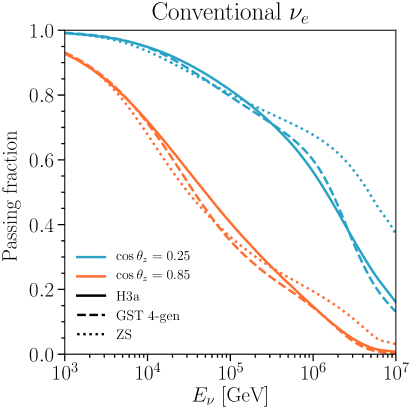
(a)

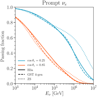
(b)

(c)

(d)

Figure 10: Passing fractions: effect of primary cosmic-ray spectrum. Results are shown for two values of $\cos\theta_{z}$ (from top to bottom): 0.25 (blue) and 0.85 (orange); for four CR models: Hillas-Gaisser H3a Gaisser (2012) (solid), Gaisser, Stanev and Tilav (GST 4-gen) Gaisser et al. (2013) (dashed) and Zatsepin-Solkolskaya (ZS) Zatsepin and Sokolskaya (2006) (dotted). Top-left panel: Conventional $\nu_{e}$ passing fraction. Top-right panel: Prompt $\nu_{e}$ passing fraction. Bottom-left panel: Conventional $\nu_{\mu}$ passing fraction. Bottom-right panel: Prompt $\nu_{\mu}$ passing fraction.

IV.2 Primary cosmic-ray spectra

Throughout this work, we have considered the Hillas-Gaisser three-population model Gaisser (2012), H3a, as a the default spectrum to show our results. In this model, each population contains five groups of nuclei which cut off exponentially at a characteristic rigidity.

An alternative model was proposed by Gaisser, Stanev, and Tilav (GST) Gaisser et al. (2013) with a much lower rigidity cutoff for the first and second populations, which have a harder spectra, and a third population with only iron above the ankle. In this model (GST 4-gen), a fourth, pure-proton population was added to obtain a better agreement with the measurements of the depth of shower maximum above $10^{9}$ GeV, which disagrees with pure iron composition. A purely proton-iron mixture, however, is also in tension with Auger data Abraham et al. (2010); Aab et al. (2014).

Another three-population model to describe the (per nucleon) energy range $(10-10^{8})$ GeV was proposed by Zatsepin and Sokolskaya (ZS) Zatsepin and Sokolskaya (2006). The first (lowest energy) component comes from expanding shells of nova explosions, the second one from explosions of isolated stars into the interstellar medium and the third (highest energy) one from explosions of massive stars into their own stellar wind, which produces a superbubble of hot and low-density gas surrounded by a shell of neutral hydrogen. Note that this model also implies a heavy composition at the highest energies.

A new data-driven phenomenological model, Global Spline Fit (GSF), has recently been proposed to describe the energy range $(10^{10}-10^{11})$ GeV Dembinski et al. (2017). It combines direct and air-shower measurements and parameterizes the cosmic-ray energy spectrum and its composition with smooth curves for all elements from proton to nickel. It is provided with a band that represents the uncertainties of the input data. As of this writing, its full implementation is not yet available in MCEQ, but once released can easily be incorporated in this framework.

In this section, we compare the atmospheric neutrino passing fractions obtained with three models of the primary cosmic-ray spectrum. The passing fractions for the conventional (left) and prompt (right) fluxes of electron (top) and muon (bottom) neutrinos are depicted in Fig. 10. As in previous figures, the comparison is shown for two zenith angles: $\cos\theta_{z}=$ 0.25 (upper and blue curves) and 0.85 (lower and orange curves). The largest variations occur for the electron neutrino flux, both conventional and prompt, although the passing fractions never have an absolute difference larger than $0.05$, except for the most horizontal trajectories when using the ZS primary cosmic-ray spectrum. In this latter case, the passing fractions are significantly larger than with the other spectra above $\sim 10^{6}$ GeV. Note, however, that the ZS spectrum does not explain the cosmic-ray data above $10^{8}$ GeV and thus, the neutrino flux is not expected to be correctly predicted above a few $10^{6}$ GeV or even lower. In the case of the conventional and prompt muon neutrino fluxes, the differences among the passing fractions using the various primary cosmic-ray spectra are much smaller. This can be understood from the importance of the correlated muon, which depends less on variations in the shower development.

Overall, systematic uncertainties from the choice of the primary cosmic-ray spectrum are non-negligible for electron neutrino passing fractions, but are small in the case of muon neutrinos.

IV.3 Hadronic-interaction models

Given the very high energies of extensive air showers produced in the atmosphere by interactions of cosmic rays, the description of the cascade development crucially relies on the theoretical modeling of hadronic interactions at these high energies which are orders of magnitude higher than those reached at colliders. Several hadronic-interaction models exist, in which contributions of soft and hard parton dynamics to inelastic hadron interactions are described within Regge field theory Gribov (1968). All these models are tuned to agree with collider data, although the predictions for the characterization of extensive air showers depend on extrapolations. Therefore, the properties of these cascades depend on the different assumptions and approaches of the models. It is important then to estimate the variations in the resulting atmospheric neutrino passing fractions depending on the hadronic-interaction model.

The default model used throughout this work for the description of multiparticle production and for the development of extensive air showers is the recently released SIBYLL 2.3c Riehn et al. (2017). This model, based on the dual parton model Capella and Krzywicki (1978); Capella and Tran Thanh Van (1981); Capella et al. (1994), represents an update from the earlier SIBYLL 2.3 Riehn et al. (2015, 2016) in order to obtain a better agreement with NA49 data Anticic et al. (2010). SIBYLL 2.3c provides a better description of kaon production spectra than previous versions Ahn et al. (2009); Riehn et al. (2015, 2016), but its predictions for the production of charmed particles and the characterization of atmospheric cascades are similar.

An alternative phenomenological model, also based on Regge field theory, is the updated quark-gluon string model with jets (QGSJET-II-04) Ostapchenko (2011), which has also been calibrated with LHC data and builds on the original QGSJET model Kalmykov et al. (1997).

A third phenomenological approach to describe cosmic-ray air shower development and heavy-ion interactions is the Monte Carlo event generator for minimum bias hadronic interactions EPOS-LHC Werner et al. (2006); Pierog et al. (2015), which is also calibrated with LHC data. The model is also based on the parton-based Regge field theory developed for NEXUS Drescher et al. (2001), which described soft interactions with the VENUS model Werner (1993) and semi-hard scattering with the QGSJET model Kalmykov et al. (1997).

Another Monte Carlo model, also based on the two-component, dual-parton model Capella and Krzywicki (1978); Capella and Tran Thanh Van (1981); Capella et al. (1994), which describes hadron-hadron, hadron-nucleus, nucleus-nucleus, and neutrino-nucleus interactions, is DPMJET-III Roesler et al. (2000). This model unifies all features of the previous event generators DPMJET-II Ranft (1995, 1999a, 1999b), DTNUC-2 Engel et al. (1997); Roesler et al. (1998), and PHOJET 1.12 Engel (1995); Engel and Ranft (1996). Within this model particle production takes place via the fragmentation of colorless parton-parton chains, which are constructed from the quark content of the interacting hadrons and nuclei. In addition to describe cosmic-ray cascade simulations, the model was also tuned to work for central collisions and to explain several features of the CERN-SPS heavy-ion data. We consider this model to calculate passing fractions for prompt atmospheric neutrinos. For conventional atmospherics, it gives similar passing fractions as SIBYLL 2.3c. Although we do not discuss it in this section, the CORSIKA simulation in Ref. Gaisser et al. (2014) used DPMJET-2.55 Berghaus et al. (2008) for prompt atmospheric neutrinos (in Fig. 9). It features, in comparison to DPMJET-II, an improved description of collision scaling in charm production and is compared with HERA-B data Abt et al. (2007).

QGSJET-II-04 is the model that predicts the smallest value for the position of the maximum in extended air showers, $X_{\rm max}$, while SIBYLL 2.3c predicts the largest $X_{\rm max}$. This has to do with the energy dependence of the inelasticity in each model Ostapchenko (2016). On another hand, SIBYLL 2.3c predicts the largest number of muons of all post-LHC models at energies above $10^{9}$ GeV, closer to the observed excess than other models Aab et al. (2015); Apel et al. (2017); Abbasi et al. (2018). Note, however, that at energies below $\sim 10^{8}$ GeV, no excess of muons has been observed Gonzalez (2016); Fomin et al. (2017), although the lateral distributions of muons are not well reproduced by most hadronic-interaction models Abbasi et al. (2013). We refer the reader to Refs. Fedynitch et al. (2012); Aab et al. (2016); Ostapchenko (2016); Riehn et al. (2017); Dedenko et al. (2017a, b); Pierog (2018) for discussions on the impact of different hadronic-interaction models on cosmic-ray data.

In Fig. 11 we compare the results for the atmospheric neutrino passing fractions using different hadronic-interaction models. We show the passing fractions for the conventional (left) and prompt (right) fluxes of electron (top) and muon (bottom) neutrinos. As in previous plots, the comparison is shown for two zenith angles: $\cos\theta_{z}=$ 0.25 (upper and blue curves) and 0.85 (lower and orange curves). For conventional neutrinos, the differences are larger for electron neutrinos. This is expected due to the more well-understood, correlated muon. All models predict similar conventional passing fractions, except QGSJET-II-04 which predicts the smallest and has an absolute difference of $\sim 0.1$. This can be understood from its harder muon spectrum Riehn et al. (2017). In the case of prompt $\nu_{e}$, the passing fractions obtained when using DPMJET-III are larger than those with SIBYLL 2.3 or SIBYLL 2.3c. For prompt $\nu_{\mu}$, the differences from model to model are negligible.

Overall, we conclude that the choice of the hadronic-interaction model introduces negligible systematic uncertainties in the passing fractions for atmospheric muon neutrinos, but they can be important for electron neutrinos.

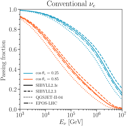
(a)

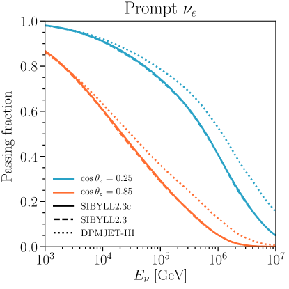
(b)

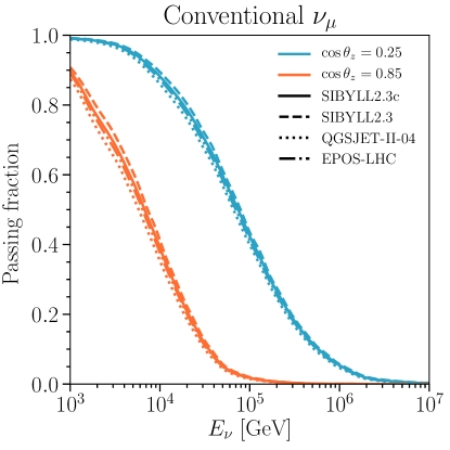
(c)

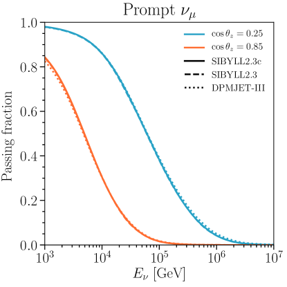
(d)

Figure 11: Passing fractions: effect of hadronic-interaction model. Results are shown for two values of $\cos\theta_{z}$ (from top to bottom): 0.25 (blue) and 0.85 (orange); for different hadronic-interaction models: SIBYLL 2.3c Riehn et al. (2017) (solid), SIBYLL 2.3 Riehn et al. (2015, 2016) (dashed), QGSJET-II-04 Ostapchenko (2011) (dotted in left panel), EPOS-LHC Pierog et al. (2015) (dash-dotted in left panel) and DPMJET-IIIRoesler et al. (2000) (dotted in right panel). Top-left panel: Conventional $\nu_{e}$ passing fraction. Top-right panel: Prompt $\nu_{e}$ passing fraction. Bottom-left panel: Conventional $\nu_{\mu}$ passing fraction. Bottom-right panel: Prompt $\nu_{\mu}$ passing fraction.

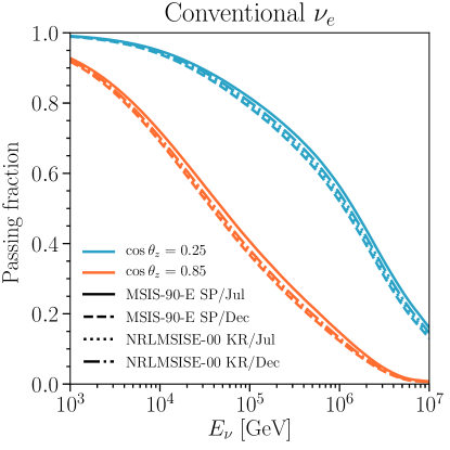
(a)

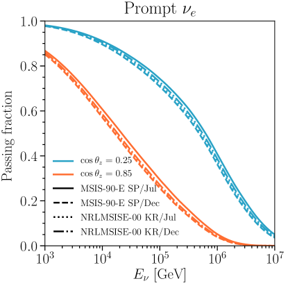
(b)

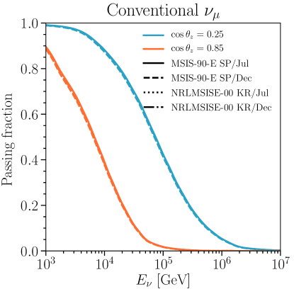
(c)

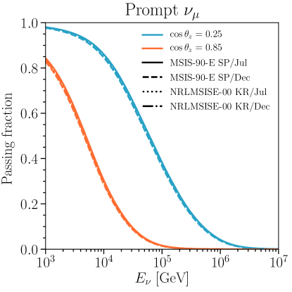
(d)

Figure 12: Passing fractions: effect of the atmosphere-density model. Results are shown for two values of $\cos\theta_{z}$ (from top to bottom): 0.25 (blue) and 0.85 (orange); for two locations: South Pole (solid and dashed) and Karlsruhe (dotted and dash-dotted); and for two different months, July (solid and dotted) and December (dashed and dash-dotted). For the South Pole calculations we use the MSIS-90-E model Labitzke et al. (1985); Hedin (1991), whereas for the Karlsruhe case we use NRLMSIS-00 Picone, J. M., Hedin, A. E., Drob, D. P. and Aikin, A. C. (2002). Top-left panel: Conventional $\nu_{e}$ passing fraction. Top-right panel: Prompt $\nu_{e}$ passing fraction. Bottom-left panel: Conventional $\nu_{\mu}$ passing fraction. Bottom-right panel: Prompt $\nu_{\mu}$ passing fraction.

IV.4 Atmosphere-density models

The two atmosphere-density models we consider are included in MCEQ, one of which is also included in CORSIKA Heck and Pierog (2018). They are five-layer profiles with a volume composition of 78.1% $N_{2}$, 21% $O_{2}$ and 0.9% $Ar$. The mass overburden of the lower four layers follows an exponential profile dependent on the altitude, while the upper layer decreases linearly with altitude up to a maximum of 112.8 km Heck et al. (1998).

All the results presented in this work have been obtained using the MSIS-90-E model Labitzke et al. (1985); Hedin (1991) for the South Pole atmosphere on July 01, 1997 Heck and Pierog (2018). This model was also used to perform the CORSIKA simulation shown in some figures in section III.

In this section we evaluate the effects of seasonal and location variations in the atmosphere on the passing fractions. To check the seasonal dependence, we consider the MSIS-90-E model for the South Pole atmosphere on December 31, 1997 Heck and Pierog (2018). To understand the dependence of our results on the atmosphere-density model, we also consider the NRLMSIS-00 empirical model Picone, J. M., Hedin, A. E., Drob, D. P. and Aikin, A. C. (2002) for the South Pole and for Karlsruhe, during summer and winter. This is a more recent model based on MSIS-90-E. In MCEQ different locations can be chosen when using NRLMSIS-00, but not MSIS-90-E.

Differences in the passing fractions from model to model are below the percent level, so we do not explicitly show them. We next study seasonal and location differences. We consider the MSIS-90-E model for the South Pole and the NRLMSIS-00 model for Karlsruhe, at two different times of the year. In Fig. 12 we illustrate how the seasonal and location variations in the atmosphere’s density affect the passing fractions. As done for other comparisons, we show the passing fractions for the conventional (left) and prompt (right) atmospheric fluxes of electron (top) and muon (bottom) neutrinos; and for two zenith angles: $\cos\theta_{z}=$ 0.25 (upper and blue curves) and 0.85 (lower and orange curves). Seasonal effects at the South Pole are not negligible for electron neutrino passing fractions, with absolute differences up to $\sim 0.05$. Seasonal variations are much smaller at Karlsruhe, which results in the electron neutrino passing fractions lying within the seasonal variations for the South Pole. Analogous to previous section discussions about the other sources of systematic uncertainties, location and seasonal differences have very little impact on the muon neutrino passing fractions.

V Detector configuration

In this work we have considered a particular, simplified, detector configuration. In the previous section we highlighted and studied the main sources of systematic uncertainties entering into the calculations. In this section we describe the different characteristics of the detector which also affects the final efficiency.

V.1 Depth

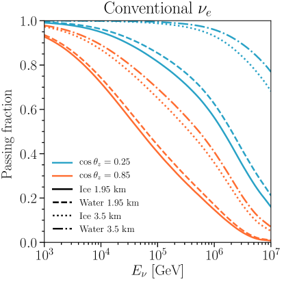
(a)

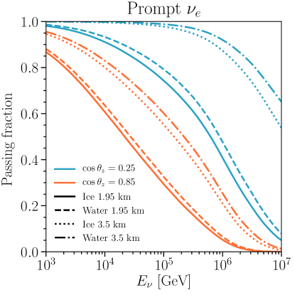
(b)

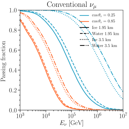
(c)

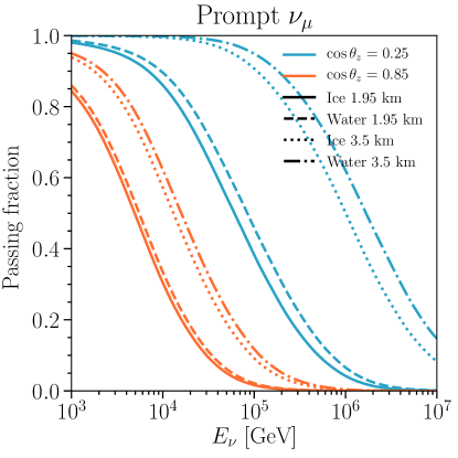
(d)

Figure 13: Passing fractions: effect of depth/medium. Results are shown for two values of $\cos\theta_{z}$ (from top to bottom): 0.25 (blue) and 0.85 (orange); for two depths: $d_{\rm det}=1.95$ km (solid and dashed) and $d_{\rm det}=3.5$ km (dotted and dash-dotted); and for two different media: ice (solid and dotted) and water (dashed and dot-dashed). Top-left panel: Conventional $\nu_{e}$ passing fraction. Top-right panel: Prompt $\nu_{e}$ passing fraction. Bottom-left panel: Conventional $\nu_{\mu}$ passing fraction. Bottom-right panel: Prompt $\nu_{\mu}$ passing fraction.

Throughout this work, we have assumed the detector’s veto to be located at a depth of 1.95 km in ice, corresponding to the center of the IceCube detector Achterberg et al. (2006). Nevertheless, the exact modeling of the veto geometry has an important impact on the calculation of the atmospheric neutrino passing fractions. To illustrate the effect of the depth, in Fig 13 we depict the passing fractions for two different values: $d_{\rm det}=1.95$ km (solid and dashed) and $d_{\rm det}=3.5$ km (dotted and dash-dotted). As in previous plots, we show the passing fractions for the conventional (left) and prompt (right) fluxes of electron (top) and muon (bottom) neutrinos; and for two zenith angles: $\cos\theta_{z}=$ 0.25 (upper and blue curves) and 0.85 (lower and orange curves). As expected, the deeper the detector is located, the more energy the muon loses, increasing the probability to not trigger the veto. Therefore, the vetoing power of this technique is reduced significantly and the atmospheric neutrino passing fractions are larger for deeper detectors. This highlights the importance of taking into account the geometry of the veto properly when applying this technique and becomes relevant for other neutrino telescopes.

V.2 Surrounding medium

In section II.2, we have described the probability for muons with a given energy at the Earth’s surface to reach and trigger the detector’s veto, ${\cal P}_{\rm det}$. This is dictated in-part by how much energy the muons lose when traversing the surrounding medium of the detector. The nature of muon energy losses depend on the medium of propagation. Although we have studied energy losses in ice in detail, which applies to the IceCube detector Achterberg et al. (2006), another type of neutrino detectors which uses water is represented by ANTARES Ageron et al. (2011) and KM3NeT Adrián-Martínez et al. (2016) in the Mediterranean sea, and by Baikal-GVD Avrorin et al. (2018) in Lake Baikal.

The KM3NeT-Italy infrastructure, at the former NEMO site, is located at a depth of 3.5 km, whereas Baikal-GVD centers at a depth of 1 km. Therefore, for an appropriate evaluation of the impact of the medium on our results, in Fig 13 we also compare the passing fractions in ice (solid and dotted) and water (dashed and dash-dotted) for the detector’s veto at depth $d_{\rm det}=1.95$ km (solid and dashed) and $d_{\rm det}=3.5$ km (dotted and dash-dotted), with the rest of the parameters and inputs fixed. We note that the differences caused by the propagation of muons in solid or liquid water are not dramatic. These differences are more pronounced for more horizontal trajectories. Conventional and prompt fluxes exhibit similar differences. Finally, even though the changes due to the propagation medium are not large, the difference in depths between IceCube and KM3NeT results in a very important reduction of rejection power for the latter. Similarly, and although not explicitly shown, the shallower location of the Baikal-GVD implies that the atmospheric neutrino passing fractions for this configuration are the smallest ones of the three cases and thus, applying this technique might be especially relevant for Baikal-GVD.

V.3 Muon veto trigger probability

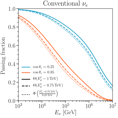
(a)

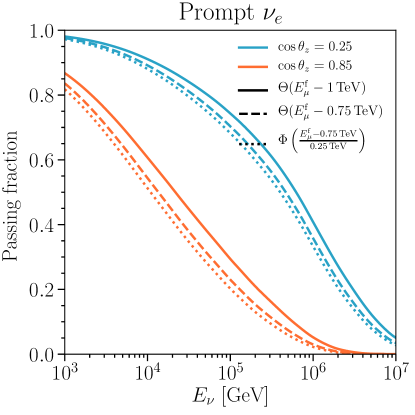
(b)

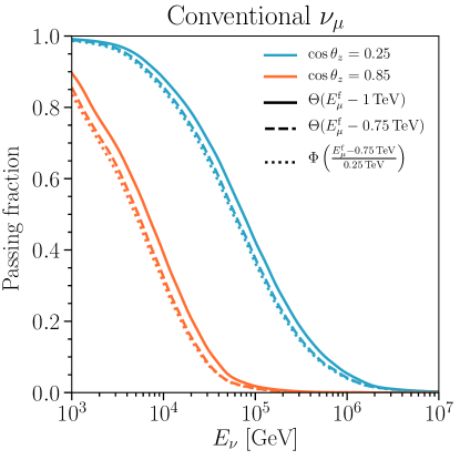
(c)

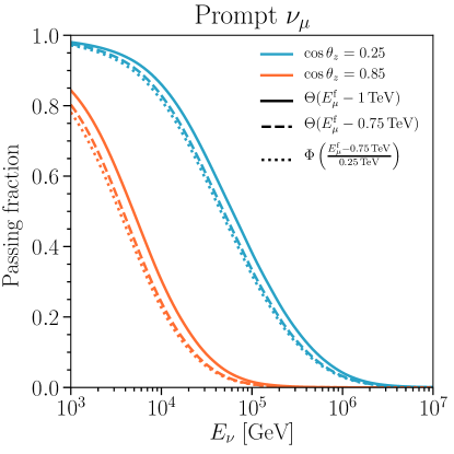
(d)

Figure 14: Passing fractions: effect of $\boldsymbol{{\cal P}_{\rm light}}$. Results are shown for two values of $\cos\theta_{z}$ (from top to bottom): 0.25 (blue) and 0.85 (orange); for three different ${\cal P}_{\rm light}(E_{\mu}^{\rm f})$: a Heaviside with a muon threshold at 1 TeV, $\Theta\left(E_{\mu}^{\rm f}-1\,{\rm TeV}\right)$ (solid), a Heaviside with a muon threshold at 0.75 TeV, $\Theta\left(E_{\mu}^{\rm f}-0.75\,{\rm TeV}\right)$ (dashed) and a sigmoid $\Phi\left(\left(E_{\mu}^{\rm f}-0.75\,{\rm TeV}\right)/0.25\,{\rm TeV}\right)$ (dotted). Top-left panel: Conventional $\nu_{e}$ passing fraction. Top-right panel: Prompt $\nu_{e}$ passing fraction. Bottom-left panel: Conventional $\nu_{\mu}$ passing fraction. Bottom-right panel: Prompt $\nu_{\mu}$ passing fraction.

Once muons reach the detector, the key quantity to determine whether they can be correlated with a neutrino event is the probability to trigger the veto, ${\cal P}_{\rm light}$. This is described in section II.2. Although we have shown ${\cal P}_{\rm det}$ for two different ${\cal P}_{\rm light}$ settings (Fig. 2), thus far we have only shown passing fractions assuming a Heaviside function. This efficiency function depends on the veto’s configuration, so it is important to study the results using different functional forms.

We illustrate the effects of the modeling of the veto’s response in Fig. 14, where we depict the passing fractions for the conventional (left) and prompt (right) fluxes of atmospheric electron (top) and muon (bottom) neutrinos, for three different forms of ${\cal P}_{\rm light}$: Heaviside with a muon threshold at 1 TeV, $\Theta\left(E_{\mu}^{\rm f}-1\,{\rm TeV}\right)$ (solid), Heaviside with a muon threshold at 0.75 TeV, $\Theta\left(E_{\mu}^{\rm f}-0.75\,{\rm TeV}\right)$ (dashed), and sigmoid $\Phi\left(\left(E_{\mu}^{\rm f}-0.75\,{\rm TeV}\right)/0.25\,{\rm TeV}\right)$ (dotted). In each plot, we show the passing fractions for two zenith angles: $\cos\theta_{z}=$ 0.25 (upper and blue curves) and 0.85 (lower and orange curves). As expected, reducing the energy threshold reduces the passing fractions, as more muons can be correlated with the neutrino event. The difference in absolute passing fractions are slightly larger for electron neutrinos, as the less energetic uncorrelated muons are more likely to trigger the veto. This effect is the largest change in passing fractions for muon neutrinos for a given detector. Combining this information with the fact that the muon neutrinos dominate the atmospheric flux implies that this small change in the passing fractions have a larger impact on the final passing rate. On the other hand, a smoother (more realistic) efficiency function around the nominal threshold energy, as described by the sigmoid, slightly reduces the passing fraction with respect to the abrupt form represented by the Heaviside function. For the examples shown, this effect is small. As discussed in section II.2, this should be revisited in the extended formalism that considers the total energy of muon bundles and their properties.

Overall, absolute changes in the passing fractions are not very large when varying the threshold energy from 1 TeV to 0.75 TeV and the effect of a smooth ${\cal P}_{\rm light}$ is also mild; as reflected by our toy ${\cal P}_{\rm light}$ studies. Note that this later statement does not imply that the change in passing flux is negligible. Finally, each experiment that uses this calculation ought to carefully estimate their ${\cal P}_{\rm light}$, and significant changes of the passing fractions presented in this work can arise due to this.

VI Discussion and conclusions

After the discovery of the first high-energy neutrinos of extraterrestrial origin by the IceCube neutrino observatory Aartsen et al. (2013a, b, 2014, 2015a, 2017, 2015b, 2016, 2015c), the next step is to accurately measure this flux and determine its cosmic origin. Accessing its contribution at lower energies would greatly help in this task and, in order to do so, a precise modeling of the background is required. In particular, a technique that substantially reduces the background atmospheric neutrino flux was proposed a few years ago Schönert et al. (2009); Gaisser et al. (2014). The idea relies on the fact that some of the muons produced in the same air shower as atmospheric neutrinos might reach the detector and trigger the veto in coincidence with the neutrino event. In this way, the atmospheric neutrino background can be significantly reduced. Building upon this idea, we have presented a new calculation of the atmospheric neutrino passing fraction, that is, the fraction of the neutrino flux that contributes to the background in searches for astrophysical neutrinos. This calculation unifies the calculation for electron and muon neutrinos and is suited for including systematic uncertainties and different detector characteristics. As a summary of our results, in Fig. 1 we have depicted the atmospheric neutrino passing fluxes for 10 TeV and 100 TeV, for conventional and prompt electron and muon neutrinos. An astrophysical $\nu_{\mu}$ flux is included for comparison Aartsen et al. (2017).

In section II.1, we indicated our default settings and the numerical tool (MCEQ) used to describe atmospheric lepton fluxes. One of the important ingredients in our calculations is the probability for a muon to reach the detector and trigger the veto, which is defined in section II.2 and shown in Fig. 2. After the preliminary descriptions, we introduced a new definition of the passing fractions for electron and muon neutrinos, and discussed the implications for tau neutrinos in section III. This is the core of this work. Our definition allows for a unified treatment of the correlated Schönert et al. (2009) and uncorrelated Gaisser et al. (2014) parts of the atmospheric neutrino passing fractions. In that section, we also studied the effect of some previous approximations and have compared our results with those from a CORSIKA simulation, finding excellent agreement. All these comparisons are depicted in Figs. 3– 5 for electron neutrinos and in Figs. 6– 8 for muon neutrinos. In general, we find non-negligible differences between our approach with and without a number of approximations. Moreover, these differences have non-trivial energy and zenith angle dependence. In section III.4, we presented the overall comparison between our results and those from the original proposal Schönert et al. (2009); Gaisser et al. (2014) (Fig. 9), with a critical discussion on the modifications and improvements.

After presenting our approach to compute the passing fractions, the second goal of this work was to evaluate how systematic uncertainties propagate into our calculations and how our results depend on the veto configuration. The former is described in section IV, where we studied the impact of different sources of systematic uncertainties: from the treatment of muon-energy losses in section IV.1, from the choice of primary cosmic-ray spectrum in section IV.2 (Fig. 10), from the choice of the hadronic-interaction model in section IV.3 (Fig. 11), and from the choice of the atmosphere-density model in section IV.4 (Fig. 12). We conclude that systematic uncertainties, for both the conventional and prompt passing fractions, are non-negligible in the case of electron neutrinos, but they are small for muon neutrinos. Notice, however, that the atmospheric muon neutrino flux is an order of magnitude larger than the electron neutrino flux at these energies. Therefore, small changes in the muon passing fractions can have more important effects on the passing fluxes than larger changes in the electron neutrino passing fraction. The detector-dependent effects on the passing fractions are discussed in section V, namely: depth of the detector in section V.1, surrounding medium in section V.2 (Fig. 13), and muon veto trigger probability of muons in section V.3 (Fig. 14). The depth of the detector has a crucial impact on our results. Therefore, the detector geometry is important. Consequently, the atmospheric neutrino passing fractions computed for different present and planned large-scale neutrino telescopes, such as IceCube Achterberg et al. (2006), ANTARES Ageron et al. (2011), KM3NeT Adrián-Martínez et al. (2016), and Baikal-GVD Avrorin et al. (2018), are significantly different. Moreover, although the medium (water or ice) is not a critical factor, the differences in the passing fractions are not negligible. Finally, we have also shown that considering different veto efficiencies for muons can have a non-negligible impact on the results; this needs to be carefully modeled by a detailed detector simulation.

The variation of the different inputs in our calculation mainly affect the prediction of the passing fractions for electrons neutrinos, while for muon neutrinos the effect tends to be smaller. Nevertheless, the final uncertainties on the passing fluxes may not be proportional to that on the passing fractions. A consistent treatment of uncertainties involves the convolution of the passing fraction and neutrino flux uncertainties, which can be easily implemented within our approach.

In this work, a new framework for calculating the atmospheric neutrino passing fractions has been proposed. Equation (III.2) unifies the formalism introduced in previous works into a fully consistent treatment for electron, muon, and tau neutrinos. Our calculation allows for easily testing the effect of different primary cosmic-ray spectra, hadronic-interaction model, atmosphere-density model, muon-energy loss, and detector configuration. To facilitate this, a new Python package is available and described in appendix A, and the results with our default settings are provided in tabulated form in appendix B. It should be a widely-applicable tool for current and future large-scale neutrino telescopes that could help to pave the road into the era of precision sub-PeV neutrino astrophysics.

Appendix A Atmospheric neutrino passing fraction code

The atmospheric neutrino passing fraction code, $\nu$eto, is a Python package that can be found at

https://github.com/tianluyuan/nuVeto/

and implements our master equations, Eqs. (13) and (III.2). It calculates the passing fraction or passing flux of atmospheric neutrinos and antineutrinos as a function of energy, flavor, zenith angle, and detector depth for any given primary flux, hadronic-interaction model, and atmosphere-density profile implemented in MCEQ. It is also possible to generate any detection probability, given by Eq. (1), for different detector configurations in water and ice using the ${\cal P}_{\rm reach}$ distributions that are provided for those two media.

The package requires MCEQ; follow the directions for installing MCEQ before trying to use the code. Another dependency that is only needed for generating Eq. (1) is pandas. Once installed, a simple example to get started is the following:

⬇

from nuVeto.nuveto import passing

enu = 1e5*Units.GeV

cos_theta = 0.5

pf = passing(enu, cos_theta, kind=‘conv_numu’,

pmodel=(pm.HillasGaisser2012, ‘H3a’),

hadr=‘SIBYLL2.3c’, depth=1950*Units.m,

density=(‘CORSIKA’, (‘SouthPole’,‘June’)))

Here, passing is a wrapper function that builds and calls the nuVeto calculation object. All parameters that affect the total flux as calculated in MCEQ are passed to the constructor of the nuVeto class, and other parameters such as the neutrino energy, zenith angle and medium, are passed directly to the calculation function nuVeto.get_fluxes. This reduces the computing time by calling MCEQ only when necessary.

Equation (1) is constructed from a convolution of ${\cal P}_{\rm reach}$ and ${\cal P}_{\rm light}$. ${\cal P}_{\rm reach}$ is provided for both water and ice in resources/mu/mmc/*.pklz. The detector response probability must be defined in resources/mu/pl.py as a function of the muon energy at the detector. The function must follow the proper format as the other functions in that file and begin with pl_, as in def pl_myplight(emu). Since this is a detector-dependent quantity, it must be computed separately from the $\nu$eto package. However, several default assumptions of ${\cal P}_{\rm light}$ are included as described in Sec. V.3. Once ${\cal P}_{\rm light}$ is defined, execute the following commands to construct and place Eq. (1) in the proper location,

⬇

cd nuVeto/resources/mu

./mu.py -o ../../prpl/mypdet.pkl --plight pl_myplight mmc/ice_allm97.pklz

To use the newly generated file, it must be passed as a string to the prpl argument,

⬇

passing(enu, cos_theta, prpl=‘mypdet’)’

Appendix B Tabulated atmospheric neutrino passing fractions

In this section we present tabulated passing fractions for our default settings in the text, namely: the H3a cosmic-ray spectrum Gaisser (2012), the SIBYLL 2.3c Riehn et al. (2017) hadronic-interaction model, and the MSIS-90-E atmosphere-density model at the South Pole on July 1, 1997 Labitzke et al. (1985); Hedin (1991). We consider a detector located in ice at a depth of $d_{\rm det}=1.95$ km. For the propagation of muons we use the default settings in MMC Chirkin and Rhode (2004). For ${\cal P}_{\rm light}$ we use a Heaviside function with a muon threshold at $E_{\mu}^{\rm th}=1$ TeV.

	$\cos\theta_{z}$
$E_{\nu}$ [GeV]	0.1	0.2	0.3	0.4	0.5	0.6	0.7	0.8	0.9	1.0
$1.0\cdot 10^{3}$	1.00	1.00	0.98	0.97	0.96	0.94	0.94	0.93	0.92	0.92
$1.6\cdot 10^{3}$	1.00	0.99	0.98	0.96	0.94	0.92	0.91	0.90	0.89	0.89
$2.6\cdot 10^{3}$	1.00	0.99	0.97	0.94	0.91	0.89	0.88	0.86	0.86	0.85
$4.3\cdot 10^{3}$	1.00	0.99	0.95	0.91	0.88	0.85	0.84	0.82	0.81	0.80
$7.0\cdot 10^{3}$	1.00	0.98	0.93	0.88	0.84	0.81	0.79	0.77	0.76	0.75
$1.1\cdot 10^{4}$	1.00	0.98	0.91	0.85	0.80	0.75	0.73	0.71	0.69	0.68
$1.8\cdot 10^{4}$	1.00	0.96	0.88	0.80	0.74	0.69	0.67	0.64	0.63	0.62
$3.0\cdot 10^{4}$	1.00	0.95	0.84	0.75	0.69	0.63	0.61	0.57	0.56	0.55
$4.8\cdot 10^{4}$	1.00	0.93	0.80	0.70	0.62	0.56	0.54	0.51	0.49	0.48
$7.8\cdot 10^{4}$	1.00	0.91	0.76	0.64	0.56	0.50	0.47	0.44	0.43	0.42
$1.3\cdot 10^{5}$	1.00	0.89	0.71	0.59	0.50	0.44	0.41	0.38	0.37	0.36
$2.1\cdot 10^{5}$	1.00	0.86	0.66	0.53	0.44	0.38	0.35	0.32	0.31	0.30
$3.4\cdot 10^{5}$	1.00	0.82	0.60	0.47	0.38	0.32	0.29	0.26	0.25	0.25
$5.5\cdot 10^{5}$	0.99	0.78	0.54	0.40	0.32	0.26	0.24	0.21	0.20	0.20
$8.9\cdot 10^{5}$	0.99	0.72	0.47	0.34	0.26	0.20	0.19	0.16	0.15	0.15
$1.4\cdot 10^{6}$	0.98	0.65	0.39	0.26	0.19	0.15	0.13	0.11	0.11	0.10
$2.3\cdot 10^{6}$	0.97	0.57	0.30	0.18	0.13	$9.3\cdot 10^{-2}$	$8.2\cdot 10^{-2}$	$6.8\cdot 10^{-2}$	$6.4\cdot 10^{-2}$	$6.1\cdot 10^{-2}$
$3.8\cdot 10^{6}$	0.96	0.48	0.21	0.11	$7.3\cdot 10^{-2}$	$4.9\cdot 10^{-2}$	$4.2\cdot 10^{-2}$	$3.4\cdot 10^{-2}$	$3.2\cdot 10^{-2}$	$3.0\cdot 10^{-2}$
$6.2\cdot 10^{6}$	0.94	0.39	0.14	$6.6\cdot 10^{-2}$	$3.7\cdot 10^{-2}$	$2.3\cdot 10^{-2}$	$1.9\cdot 10^{-2}$	$1.4\cdot 10^{-2}$	$1.3\cdot 10^{-2}$	$1.2\cdot 10^{-2}$
$1.0\cdot 10^{7}$	0.91	0.30	$8.9\cdot 10^{-2}$	$3.8\cdot 10^{-2}$	$2.0\cdot 10^{-2}$	$1.2\cdot 10^{-2}$	$9.8\cdot 10^{-3}$	$7.4\cdot 10^{-3}$	$6.8\cdot 10^{-3}$	$6.4\cdot 10^{-3}$

Table 1: Conventional electron neutrino passing fraction for $E_{\nu}=[10^{3},\,10^{7}]$ GeV and $\cos\theta_{z}=[0.1,\,1.0]$.

	$\cos\theta_{z}$
$E_{\nu}$ [GeV]	0.1	0.2	0.3	0.4	0.5	0.6	0.7	0.8	0.9	1.0
$1.0\cdot 10^{3}$	1.00	1.00	0.98	0.96	0.95	0.93	0.93	0.92	0.91	0.91
$1.6\cdot 10^{3}$	1.00	0.99	0.97	0.95	0.93	0.91	0.90	0.88	0.88	0.87
$2.6\cdot 10^{3}$	1.00	0.99	0.96	0.93	0.90	0.87	0.86	0.84	0.83	0.83
$4.3\cdot 10^{3}$	1.00	0.99	0.94	0.90	0.86	0.83	0.81	0.79	0.78	0.77
$7.0\cdot 10^{3}$	1.00	0.98	0.92	0.87	0.82	0.78	0.76	0.74	0.73	0.72
$1.1\cdot 10^{4}$	1.00	0.97	0.89	0.82	0.77	0.72	0.70	0.67	0.66	0.65
$1.8\cdot 10^{4}$	1.00	0.96	0.86	0.78	0.71	0.66	0.64	0.61	0.59	0.58
$3.0\cdot 10^{4}$	1.00	0.94	0.82	0.73	0.65	0.60	0.57	0.54	0.53	0.52
$4.8\cdot 10^{4}$	1.00	0.92	0.78	0.67	0.59	0.53	0.50	0.47	0.46	0.45
$7.8\cdot 10^{4}$	1.00	0.90	0.73	0.61	0.53	0.46	0.44	0.41	0.39	0.38
$1.3\cdot 10^{5}$	1.00	0.88	0.68	0.55	0.47	0.40	0.38	0.35	0.33	0.32
$2.1\cdot 10^{5}$	1.00	0.84	0.63	0.50	0.41	0.34	0.32	0.29	0.28	0.27
$3.4\cdot 10^{5}$	1.00	0.80	0.57	0.43	0.35	0.29	0.26	0.23	0.22	0.22
$5.5\cdot 10^{5}$	0.99	0.76	0.51	0.37	0.29	0.23	0.21	0.18	0.17	0.17
$8.9\cdot 10^{5}$	0.99	0.70	0.43	0.30	0.22	0.17	0.16	0.13	0.13	0.12
$1.4\cdot 10^{6}$	0.98	0.62	0.35	0.22	0.16	0.12	0.11	$8.8\cdot 10^{-2}$	$8.3\cdot 10^{-2}$	$7.9\cdot 10^{-2}$
$2.3\cdot 10^{6}$	0.97	0.53	0.26	0.15	0.10	$7.1\cdot 10^{-2}$	$6.2\cdot 10^{-2}$	$5.1\cdot 10^{-2}$	$4.7\cdot 10^{-2}$	$4.5\cdot 10^{-2}$
$3.8\cdot 10^{6}$	0.95	0.44	0.18	$9.1\cdot 10^{-2}$	$5.5\cdot 10^{-2}$	$3.6\cdot 10^{-2}$	$3.0\cdot 10^{-2}$	$2.4\cdot 10^{-2}$	$2.2\cdot 10^{-2}$	$2.1\cdot 10^{-2}$
$6.2\cdot 10^{6}$	0.93	0.35	0.11	$5.1\cdot 10^{-2}$	$2.7\cdot 10^{-2}$	$1.6\cdot 10^{-2}$	$1.3\cdot 10^{-2}$	$9.4\cdot 10^{-3}$	$8.5\cdot 10^{-3}$	$7.9\cdot 10^{-3}$
$1.0\cdot 10^{7}$	0.89	0.26	$6.9\cdot 10^{-2}$	$2.7\cdot 10^{-2}$	$1.3\cdot 10^{-2}$	$7.5\cdot 10^{-3}$	$6.0\cdot 10^{-3}$	$4.4\cdot 10^{-3}$	$4.0\cdot 10^{-3}$	$3.7\cdot 10^{-3}$

Table 2: Conventional electron antineutrino passing fraction for $E_{\nu}=[10^{3},\,10^{7}]$ GeV and $\cos\theta_{z}=[0.1,\,1.0]$.

	$\cos\theta_{z}$
$E_{\nu}$ [GeV]	0.1	0.2	0.3	0.4	0.5	0.6	0.7	0.8	0.9	1.0
$1.0\cdot 10^{3}$	1.00	1.00	0.98	0.97	0.95	0.93	0.92	0.90	0.89	0.87
$1.6\cdot 10^{3}$	1.00	0.99	0.98	0.95	0.91	0.88	0.85	0.82	0.79	0.78
$2.6\cdot 10^{3}$	1.00	0.99	0.96	0.90	0.84	0.79	0.76	0.73	0.71	0.69
$4.3\cdot 10^{3}$	1.00	0.99	0.92	0.83	0.76	0.70	0.67	0.63	0.60	0.58
$7.0\cdot 10^{3}$	1.00	0.97	0.86	0.75	0.67	0.59	0.55	0.50	0.47	0.44
$1.1\cdot 10^{4}$	1.00	0.94	0.79	0.65	0.55	0.47	0.42	0.37	0.34	0.31
$1.8\cdot 10^{4}$	1.00	0.90	0.70	0.54	0.42	0.33	0.28	0.24	0.21	0.19
$3.0\cdot 10^{4}$	1.00	0.85	0.59	0.40	0.29	0.21	0.17	0.14	0.11	$9.5\cdot 10^{-2}$
$4.8\cdot 10^{4}$	1.00	0.77	0.46	0.28	0.18	0.12	$8.7\cdot 10^{-2}$	$6.2\cdot 10^{-2}$	$4.9\cdot 10^{-2}$	$3.9\cdot 10^{-2}$
$7.8\cdot 10^{4}$	1.00	0.69	0.35	0.18	0.10	$5.8\cdot 10^{-2}$	$4.1\cdot 10^{-2}$	$3.0\cdot 10^{-2}$	$2.4\cdot 10^{-2}$	$1.9\cdot 10^{-2}$
$1.3\cdot 10^{5}$	0.99	0.58	0.24	0.10	$5.5\cdot 10^{-2}$	$2.8\cdot 10^{-2}$	$2.1\cdot 10^{-2}$	$1.5\cdot 10^{-2}$	$1.2\cdot 10^{-2}$	$9.3\cdot 10^{-3}$
$2.1\cdot 10^{5}$	0.98	0.46	0.15	$5.7\cdot 10^{-2}$	$3.0\cdot 10^{-2}$	$1.4\cdot 10^{-2}$	$1.0\cdot 10^{-2}$	$7.3\cdot 10^{-3}$	$6.0\cdot 10^{-3}$	$4.3\cdot 10^{-3}$
$3.4\cdot 10^{5}$	0.96	0.35	$9.0\cdot 10^{-2}$	$3.0\cdot 10^{-2}$	$1.5\cdot 10^{-2}$	$6.4\cdot 10^{-3}$	$4.5\cdot 10^{-3}$	$3.3\cdot 10^{-3}$	$2.7\cdot 10^{-3}$	$1.9\cdot 10^{-3}$
$5.5\cdot 10^{5}$	0.93	0.25	$5.1\cdot 10^{-2}$	$1.4\cdot 10^{-2}$	$6.5\cdot 10^{-3}$	$1.8\cdot 10^{-3}$	$1.2\cdot 10^{-3}$	$1.1\cdot 10^{-3}$	$7.8\cdot 10^{-4}$	$5.4\cdot 10^{-4}$
$8.9\cdot 10^{5}$	0.90	0.17	$2.7\cdot 10^{-2}$	$5.0\cdot 10^{-3}$	$1.8\cdot 10^{-3}$	$8.2\cdot 10^{-4}$	$4.7\cdot 10^{-4}$	$2.8\cdot 10^{-4}$	$2.3\cdot 10^{-4}$	$1.4\cdot 10^{-4}$
$1.4\cdot 10^{6}$	0.84	0.11	$1.0\cdot 10^{-2}$	$2.7\cdot 10^{-3}$	$9.8\cdot 10^{-4}$	$4.5\cdot 10^{-4}$	$2.3\cdot 10^{-4}$	$1.4\cdot 10^{-4}$	$1.1\cdot 10^{-4}$	$9.0\cdot 10^{-5}$
$2.3\cdot 10^{6}$	0.77	$6.2\cdot 10^{-2}$	$6.0\cdot 10^{-3}$	$1.4\cdot 10^{-3}$	$5.1\cdot 10^{-4}$	$2.2\cdot 10^{-4}$	$1.2\cdot 10^{-4}$	$6.1\cdot 10^{-5}$	$3.8\cdot 10^{-5}$	$4.3\cdot 10^{-5}$
$3.8\cdot 10^{6}$	0.69	$3.0\cdot 10^{-2}$	$3.1\cdot 10^{-3}$	$6.2\cdot 10^{-4}$	$2.1\cdot 10^{-4}$	$8.6\cdot 10^{-5}$	$5.7\cdot 10^{-5}$	$2.3\cdot 10^{-5}$	$1.1\cdot 10^{-5}$	$1.9\cdot 10^{-5}$
$6.2\cdot 10^{6}$	0.59	$1.8\cdot 10^{-2}$	$1.5\cdot 10^{-3}$	$2.5\cdot 10^{-4}$	$7.6\cdot 10^{-5}$	$2.6\cdot 10^{-5}$	$2.0\cdot 10^{-5}$	$7.5\cdot 10^{-6}$	$2.1\cdot 10^{-6}$	$6.2\cdot 10^{-6}$
$1.0\cdot 10^{7}$	0.50	$1.1\cdot 10^{-2}$	$6.7\cdot 10^{-4}$	$1.1\cdot 10^{-4}$	$2.4\cdot 10^{-5}$	$8.9\cdot 10^{-6}$	$5.7\cdot 10^{-6}$	$3.3\cdot 10^{-6}$	$7.6\cdot 10^{-7}$	$1.7\cdot 10^{-6}$

Table 3: Conventional muon neutrino passing fraction for $E_{\nu}=[10^{3},\,10^{7}]$ GeV and $\cos\theta_{z}=[0.1,\,1.0]$.

	$\cos\theta_{z}$
$E_{\nu}$ [GeV]	0.1	0.2	0.3	0.4	0.5	0.6	0.7	0.8	0.9	1.0
$1.0\cdot 10^{3}$	1.00	0.99	0.98	0.95	0.93	0.91	0.89	0.87	0.85	0.83
$1.6\cdot 10^{3}$	1.00	0.99	0.96	0.93	0.89	0.84	0.80	0.76	0.74	0.71
$2.6\cdot 10^{3}$	1.00	0.99	0.94	0.87	0.80	0.73	0.70	0.66	0.64	0.62
$4.3\cdot 10^{3}$	1.00	0.98	0.89	0.78	0.70	0.64	0.60	0.57	0.54	0.52
$7.0\cdot 10^{3}$	1.00	0.96	0.82	0.70	0.61	0.54	0.49	0.45	0.42	0.39
$1.1\cdot 10^{4}$	1.00	0.93	0.74	0.60	0.50	0.41	0.37	0.32	0.29	0.27
$1.8\cdot 10^{4}$	1.00	0.88	0.65	0.49	0.38	0.29	0.25	0.21	0.18	0.16
$3.0\cdot 10^{4}$	1.00	0.82	0.55	0.36	0.26	0.18	0.15	0.12	$9.7\cdot 10^{-2}$	$8.0\cdot 10^{-2}$
$4.8\cdot 10^{4}$	1.00	0.74	0.42	0.25	0.16	0.10	$7.3\cdot 10^{-2}$	$5.2\cdot 10^{-2}$	$4.1\cdot 10^{-2}$	$3.2\cdot 10^{-2}$
$7.8\cdot 10^{4}$	0.99	0.66	0.32	0.16	$8.8\cdot 10^{-2}$	$4.8\cdot 10^{-2}$	$3.4\cdot 10^{-2}$	$2.4\cdot 10^{-2}$	$1.9\cdot 10^{-2}$	$1.5\cdot 10^{-2}$
$1.3\cdot 10^{5}$	0.99	0.55	0.21	$8.9\cdot 10^{-2}$	$4.6\cdot 10^{-2}$	$2.3\cdot 10^{-2}$	$1.7\cdot 10^{-2}$	$1.2\cdot 10^{-2}$	$9.5\cdot 10^{-3}$	$7.2\cdot 10^{-3}$
$2.1\cdot 10^{5}$	0.97	0.44	0.13	$4.9\cdot 10^{-2}$	$2.4\cdot 10^{-2}$	$1.1\cdot 10^{-2}$	$7.8\cdot 10^{-3}$	$5.5\cdot 10^{-3}$	$4.6\cdot 10^{-3}$	$3.2\cdot 10^{-3}$
$3.4\cdot 10^{5}$	0.96	0.33	$7.9\cdot 10^{-2}$	$2.5\cdot 10^{-2}$	$1.2\cdot 10^{-2}$	$4.9\cdot 10^{-3}$	$3.4\cdot 10^{-3}$	$2.4\cdot 10^{-3}$	$1.9\cdot 10^{-3}$	$1.4\cdot 10^{-3}$
$5.5\cdot 10^{5}$	0.93	0.23	$4.3\cdot 10^{-2}$	$1.1\cdot 10^{-2}$	$4.9\cdot 10^{-3}$	$1.3\cdot 10^{-3}$	$8.6\cdot 10^{-4}$	$7.7\cdot 10^{-4}$	$5.3\cdot 10^{-4}$	$3.6\cdot 10^{-4}$
$8.9\cdot 10^{5}$	0.88	0.15	$2.2\cdot 10^{-2}$	$3.7\cdot 10^{-3}$	$1.3\cdot 10^{-3}$	$5.2\cdot 10^{-4}$	$2.9\cdot 10^{-4}$	$1.7\cdot 10^{-4}$	$1.4\cdot 10^{-4}$	$8.1\cdot 10^{-5}$
$1.4\cdot 10^{6}$	0.83	$9.3\cdot 10^{-2}$	$7.6\cdot 10^{-3}$	$1.8\cdot 10^{-3}$	$5.8\cdot 10^{-4}$	$2.5\cdot 10^{-4}$	$1.2\cdot 10^{-4}$	$7.1\cdot 10^{-5}$	$5.3\cdot 10^{-5}$	$4.2\cdot 10^{-5}$
$2.3\cdot 10^{6}$	0.75	$5.1\cdot 10^{-2}$	$4.0\cdot 10^{-3}$	$7.9\cdot 10^{-4}$	$2.5\cdot 10^{-4}$	$9.8\cdot 10^{-5}$	$5.0\cdot 10^{-5}$	$2.4\cdot 10^{-5}$	$1.5\cdot 10^{-5}$	$1.5\cdot 10^{-5}$
$3.8\cdot 10^{6}$	0.66	$2.4\cdot 10^{-2}$	$1.9\cdot 10^{-3}$	$3.0\cdot 10^{-4}$	$8.6\cdot 10^{-5}$	$2.9\cdot 10^{-5}$	$1.8\cdot 10^{-5}$	$6.4\cdot 10^{-6}$	$3.0\cdot 10^{-6}$	$4.9\cdot 10^{-6}$
$6.2\cdot 10^{6}$	0.56	$1.3\cdot 10^{-2}$	$8.1\cdot 10^{-4}$	$9.9\cdot 10^{-5}$	$2.2\cdot 10^{-5}$	$6.2\cdot 10^{-6}$	$4.0\cdot 10^{-6}$	$1.3\cdot 10^{-6}$	$3.7\cdot 10^{-7}$	$9.7\cdot 10^{-7}$
$1.0\cdot 10^{7}$	0.47	$7.5\cdot 10^{-3}$	$3.0\cdot 10^{-4}$	$3.4\cdot 10^{-5}$	$5.8\cdot 10^{-6}$	$1.6\cdot 10^{-6}$	$1.1\cdot 10^{-6}$	$4.2\cdot 10^{-7}$	$8.7\cdot 10^{-8}$	$2.6\cdot 10^{-7}$

Table 4: Conventional muon antineutrino passing fraction for $E_{\nu}=[10^{3},\,10^{7}]$ GeV and $\cos\theta_{z}=[0.1,\,1.0]$.

	$\cos\theta_{z}$
$E_{\nu}$ [GeV]	0.1	0.2	0.3	0.4	0.5	0.6	0.7	0.8	0.9	1.0
$1.0\cdot 10^{3}$	1.00	0.99	0.97	0.94	0.92	0.89	0.88	0.87	0.86	0.86
$1.6\cdot 10^{3}$	1.00	0.99	0.95	0.92	0.89	0.86	0.85	0.83	0.82	0.81
$2.6\cdot 10^{3}$	1.00	0.98	0.94	0.89	0.85	0.82	0.80	0.78	0.77	0.76
$4.3\cdot 10^{3}$	1.00	0.98	0.91	0.85	0.81	0.77	0.75	0.72	0.71	0.70
$7.0\cdot 10^{3}$	1.00	0.97	0.88	0.81	0.76	0.71	0.69	0.66	0.65	0.64
$1.1\cdot 10^{4}$	1.00	0.95	0.85	0.77	0.70	0.65	0.63	0.59	0.58	0.57
$1.8\cdot 10^{4}$	1.00	0.94	0.81	0.72	0.64	0.58	0.56	0.53	0.51	0.50
$3.0\cdot 10^{4}$	1.00	0.92	0.77	0.66	0.58	0.52	0.49	0.46	0.45	0.44
$4.8\cdot 10^{4}$	1.00	0.90	0.72	0.60	0.52	0.45	0.43	0.39	0.38	0.37
$7.8\cdot 10^{4}$	1.00	0.87	0.67	0.54	0.45	0.39	0.36	0.33	0.32	0.31
$1.3\cdot 10^{5}$	1.00	0.84	0.61	0.48	0.39	0.32	0.30	0.27	0.26	0.25
$2.1\cdot 10^{5}$	1.00	0.80	0.55	0.41	0.33	0.26	0.24	0.21	0.20	0.19
$3.4\cdot 10^{5}$	0.99	0.74	0.48	0.34	0.26	0.20	0.18	0.16	0.15	0.14
$5.5\cdot 10^{5}$	0.99	0.68	0.41	0.27	0.20	0.14	0.13	0.11	0.10	$9.5\cdot 10^{-2}$
$8.9\cdot 10^{5}$	0.98	0.60	0.31	0.19	0.13	$8.9\cdot 10^{-2}$	$7.7\cdot 10^{-2}$	$6.2\cdot 10^{-2}$	$5.8\cdot 10^{-2}$	$5.4\cdot 10^{-2}$
$1.4\cdot 10^{6}$	0.96	0.50	0.22	0.12	$7.3\cdot 10^{-2}$	$4.6\cdot 10^{-2}$	$3.8\cdot 10^{-2}$	$3.0\cdot 10^{-2}$	$2.7\cdot 10^{-2}$	$2.5\cdot 10^{-2}$
$2.3\cdot 10^{6}$	0.94	0.41	0.14	$6.6\cdot 10^{-2}$	$3.5\cdot 10^{-2}$	$2.0\cdot 10^{-2}$	$1.6\cdot 10^{-2}$	$1.2\cdot 10^{-2}$	$1.1\cdot 10^{-2}$	$9.9\cdot 10^{-3}$
$3.8\cdot 10^{6}$	0.92	0.32	$8.9\cdot 10^{-2}$	$3.3\cdot 10^{-2}$	$1.5\cdot 10^{-2}$	$7.8\cdot 10^{-3}$	$6.0\cdot 10^{-3}$	$4.1\cdot 10^{-3}$	$3.6\cdot 10^{-3}$	$3.3\cdot 10^{-3}$
$6.2\cdot 10^{6}$	0.88	0.22	$4.6\cdot 10^{-2}$	$1.4\cdot 10^{-2}$	$5.3\cdot 10^{-3}$	$2.3\cdot 10^{-3}$	$1.6\cdot 10^{-3}$	$1.0\cdot 10^{-3}$	$8.6\cdot 10^{-4}$	$7.7\cdot 10^{-4}$
$1.0\cdot 10^{7}$	0.84	0.14	$2.0\cdot 10^{-2}$	$4.9\cdot 10^{-3}$	$1.6\cdot 10^{-3}$	$5.9\cdot 10^{-4}$	$4.0\cdot 10^{-4}$	$2.3\cdot 10^{-4}$	$1.9\cdot 10^{-4}$	$1.7\cdot 10^{-4}$

Table 5: Prompt electron neutrino passing fraction for $E_{\nu}=[10^{3},\,10^{7}]$ GeV and $\cos\theta_{z}=[0.1,\,1.0]$.

	$\cos\theta_{z}$
$E_{\nu}$ [GeV]	0.1	0.2	0.3	0.4	0.5	0.6	0.7	0.8	0.9	1.0
$1.0\cdot 10^{3}$	1.00	0.99	0.97	0.94	0.92	0.90	0.89	0.87	0.87	0.86
$1.6\cdot 10^{3}$	1.00	0.99	0.95	0.92	0.89	0.86	0.85	0.83	0.82	0.81
$2.6\cdot 10^{3}$	1.00	0.98	0.94	0.89	0.85	0.82	0.80	0.78	0.77	0.76
$4.3\cdot 10^{3}$	1.00	0.98	0.91	0.86	0.81	0.77	0.75	0.72	0.71	0.70
$7.0\cdot 10^{3}$	1.00	0.97	0.89	0.81	0.76	0.71	0.69	0.66	0.65	0.64
$1.1\cdot 10^{4}$	1.00	0.95	0.85	0.77	0.70	0.65	0.63	0.60	0.59	0.57
$1.8\cdot 10^{4}$	1.00	0.94	0.81	0.72	0.65	0.59	0.56	0.53	0.52	0.51
$3.0\cdot 10^{4}$	1.00	0.92	0.77	0.66	0.59	0.52	0.50	0.46	0.45	0.44
$4.8\cdot 10^{4}$	1.00	0.90	0.72	0.60	0.52	0.45	0.43	0.40	0.38	0.37
$7.8\cdot 10^{4}$	1.00	0.87	0.67	0.54	0.46	0.39	0.37	0.33	0.32	0.31
$1.3\cdot 10^{5}$	1.00	0.84	0.62	0.48	0.39	0.33	0.30	0.27	0.26	0.25
$2.1\cdot 10^{5}$	1.00	0.80	0.56	0.42	0.33	0.27	0.24	0.21	0.20	0.20
$3.4\cdot 10^{5}$	0.99	0.75	0.49	0.35	0.26	0.20	0.18	0.16	0.15	0.14
$5.5\cdot 10^{5}$	0.99	0.68	0.41	0.27	0.20	0.15	0.13	0.11	0.10	$9.7\cdot 10^{-2}$
$8.9\cdot 10^{5}$	0.98	0.60	0.32	0.20	0.13	$9.4\cdot 10^{-2}$	$8.1\cdot 10^{-2}$	$6.6\cdot 10^{-2}$	$6.2\cdot 10^{-2}$	$5.8\cdot 10^{-2}$
$1.4\cdot 10^{6}$	0.96	0.51	0.23	0.12	$7.6\cdot 10^{-2}$	$5.0\cdot 10^{-2}$	$4.2\cdot 10^{-2}$	$3.3\cdot 10^{-2}$	$3.0\cdot 10^{-2}$	$2.8\cdot 10^{-2}$
$2.3\cdot 10^{6}$	0.95	0.41	0.15	$6.8\cdot 10^{-2}$	$3.7\cdot 10^{-2}$	$2.2\cdot 10^{-2}$	$1.8\cdot 10^{-2}$	$1.3\cdot 10^{-2}$	$1.2\cdot 10^{-2}$	$1.1\cdot 10^{-2}$
$3.8\cdot 10^{6}$	0.92	0.32	$9.2\cdot 10^{-2}$	$3.6\cdot 10^{-2}$	$1.8\cdot 10^{-2}$	$9.8\cdot 10^{-3}$	$7.8\cdot 10^{-3}$	$5.6\cdot 10^{-3}$	$5.1\cdot 10^{-3}$	$4.7\cdot 10^{-3}$
$6.2\cdot 10^{6}$	0.88	0.23	$4.9\cdot 10^{-2}$	$1.6\cdot 10^{-2}$	$6.8\cdot 10^{-3}$	$3.4\cdot 10^{-3}$	$2.6\cdot 10^{-3}$	$1.9\cdot 10^{-3}$	$1.7\cdot 10^{-3}$	$1.6\cdot 10^{-3}$
$1.0\cdot 10^{7}$	0.84	0.15	$2.4\cdot 10^{-2}$	$6.5\cdot 10^{-3}$	$2.7\cdot 10^{-3}$	$1.4\cdot 10^{-3}$	$1.1\cdot 10^{-3}$	$8.6\cdot 10^{-4}$	$8.0\cdot 10^{-4}$	$7.6\cdot 10^{-4}$

Table 6: Prompt electron antineutrino passing fraction for $E_{\nu}=[10^{3},\,10^{7}]$ GeV and $\cos\theta_{z}=[0.1,\,1.0]$.

	$\cos\theta_{z}$
$E_{\nu}$ [GeV]	0.1	0.2	0.3	0.4	0.5	0.6	0.7	0.8	0.9	1.0
$1.0\cdot 10^{3}$	1.00	0.99	0.97	0.94	0.91	0.88	0.87	0.85	0.84	0.82
$1.6\cdot 10^{3}$	1.00	0.99	0.95	0.91	0.87	0.83	0.81	0.78	0.76	0.74
$2.6\cdot 10^{3}$	1.00	0.98	0.93	0.86	0.81	0.75	0.71	0.68	0.65	0.63
$4.3\cdot 10^{3}$	1.00	0.97	0.89	0.80	0.72	0.64	0.60	0.55	0.52	0.49
$7.0\cdot 10^{3}$	1.00	0.96	0.83	0.70	0.60	0.51	0.46	0.41	0.38	0.36
$1.1\cdot 10^{4}$	1.00	0.93	0.75	0.59	0.47	0.38	0.33	0.29	0.26	0.24
$1.8\cdot 10^{4}$	1.00	0.89	0.64	0.46	0.35	0.26	0.22	0.18	0.16	0.15
$3.0\cdot 10^{4}$	1.00	0.83	0.53	0.34	0.24	0.17	0.14	0.11	$9.3\cdot 10^{-2}$	$8.0\cdot 10^{-2}$
$4.8\cdot 10^{4}$	1.00	0.74	0.41	0.24	0.15	$9.8\cdot 10^{-2}$	$7.6\cdot 10^{-2}$	$5.7\cdot 10^{-2}$	$4.8\cdot 10^{-2}$	$3.9\cdot 10^{-2}$
$7.8\cdot 10^{4}$	1.00	0.65	0.30	0.15	$8.9\cdot 10^{-2}$	$5.2\cdot 10^{-2}$	$3.8\cdot 10^{-2}$	$2.7\cdot 10^{-2}$	$2.2\cdot 10^{-2}$	$1.7\cdot 10^{-2}$
$1.3\cdot 10^{5}$	0.99	0.54	0.21	$9.0\cdot 10^{-2}$	$4.7\cdot 10^{-2}$	$2.4\cdot 10^{-2}$	$1.7\cdot 10^{-2}$	$1.2\cdot 10^{-2}$	$9.6\cdot 10^{-3}$	$7.4\cdot 10^{-3}$
$2.1\cdot 10^{5}$	0.98	0.43	0.13	$5.0\cdot 10^{-2}$	$2.4\cdot 10^{-2}$	$1.1\cdot 10^{-2}$	$7.9\cdot 10^{-3}$	$5.4\cdot 10^{-3}$	$4.4\cdot 10^{-3}$	$3.3\cdot 10^{-3}$
$3.4\cdot 10^{5}$	0.96	0.32	$7.8\cdot 10^{-2}$	$2.5\cdot 10^{-2}$	$1.1\cdot 10^{-2}$	$4.8\cdot 10^{-3}$	$3.3\cdot 10^{-3}$	$2.3\cdot 10^{-3}$	$1.8\cdot 10^{-3}$	$1.3\cdot 10^{-3}$
$5.5\cdot 10^{5}$	0.93	0.23	$4.2\cdot 10^{-2}$	$1.2\cdot 10^{-2}$	$5.0\cdot 10^{-3}$	$1.9\cdot 10^{-3}$	$1.3\cdot 10^{-3}$	$8.7\cdot 10^{-4}$	$6.7\cdot 10^{-4}$	$4.8\cdot 10^{-4}$
$8.9\cdot 10^{5}$	0.88	0.14	$2.1\cdot 10^{-2}$	$4.8\cdot 10^{-3}$	$1.8\cdot 10^{-3}$	$5.9\cdot 10^{-4}$	$3.7\cdot 10^{-4}$	$2.5\cdot 10^{-4}$	$1.9\cdot 10^{-4}$	$1.3\cdot 10^{-4}$
$1.4\cdot 10^{6}$	0.81	$8.4\cdot 10^{-2}$	$8.6\cdot 10^{-3}$	$1.5\cdot 10^{-3}$	$4.9\cdot 10^{-4}$	$1.6\cdot 10^{-4}$	$9.1\cdot 10^{-5}$	$5.1\cdot 10^{-5}$	$3.9\cdot 10^{-5}$	$2.7\cdot 10^{-5}$
$2.3\cdot 10^{6}$	0.73	$4.5\cdot 10^{-2}$	$3.1\cdot 10^{-3}$	$5.0\cdot 10^{-4}$	$1.4\cdot 10^{-4}$	$4.2\cdot 10^{-5}$	$2.2\cdot 10^{-5}$	$1.0\cdot 10^{-5}$	$7.1\cdot 10^{-6}$	$6.0\cdot 10^{-6}$
$3.8\cdot 10^{6}$	0.64	$2.3\cdot 10^{-2}$	$1.2\cdot 10^{-3}$	$1.5\cdot 10^{-4}$	$3.5\cdot 10^{-5}$	$1.0\cdot 10^{-5}$	$5.6\cdot 10^{-6}$	$2.3\cdot 10^{-6}$	$1.3\cdot 10^{-6}$	$1.5\cdot 10^{-6}$
$6.2\cdot 10^{6}$	0.55	$1.1\cdot 10^{-2}$	$4.4\cdot 10^{-4}$	$4.7\cdot 10^{-5}$	$9.4\cdot 10^{-6}$	$2.4\cdot 10^{-6}$	$1.2\cdot 10^{-6}$	$4.6\cdot 10^{-7}$	$2.1\cdot 10^{-7}$	$3.0\cdot 10^{-7}$
$1.0\cdot 10^{7}$	0.45	$4.6\cdot 10^{-3}$	$1.4\cdot 10^{-4}$	$1.1\cdot 10^{-5}$	$1.6\cdot 10^{-6}$	$3.5\cdot 10^{-7}$	$1.6\cdot 10^{-7}$	$6.1\cdot 10^{-8}$	$1.7\cdot 10^{-8}$	$3.1\cdot 10^{-8}$

Table 7: Prompt muon neutrino passing fraction for $E_{\nu}=[10^{3},\,10^{7}]$ GeV and $\cos\theta_{z}=[0.1,\,1.0]$.

	$\cos\theta_{z}$
$E_{\nu}$ [GeV]	0.1	0.2	0.3	0.4	0.5	0.6	0.7	0.8	0.9	1.0
$1.0\cdot 10^{3}$	1.00	0.99	0.97	0.94	0.91	0.88	0.87	0.85	0.84	0.83
$1.6\cdot 10^{3}$	1.00	0.99	0.95	0.91	0.87	0.83	0.81	0.78	0.76	0.75
$2.6\cdot 10^{3}$	1.00	0.98	0.93	0.86	0.81	0.75	0.72	0.68	0.65	0.63
$4.3\cdot 10^{3}$	1.00	0.97	0.89	0.80	0.72	0.64	0.60	0.55	0.52	0.49
$7.0\cdot 10^{3}$	1.00	0.96	0.83	0.70	0.60	0.51	0.46	0.41	0.38	0.36
$1.1\cdot 10^{4}$	1.00	0.93	0.75	0.59	0.47	0.38	0.33	0.29	0.26	0.24
$1.8\cdot 10^{4}$	1.00	0.89	0.64	0.46	0.35	0.26	0.22	0.18	0.16	0.15
$3.0\cdot 10^{4}$	1.00	0.83	0.53	0.34	0.24	0.17	0.14	0.11	$9.4\cdot 10^{-2}$	$8.1\cdot 10^{-2}$
$4.8\cdot 10^{4}$	1.00	0.74	0.41	0.24	0.15	$9.8\cdot 10^{-2}$	$7.6\cdot 10^{-2}$	$5.8\cdot 10^{-2}$	$4.8\cdot 10^{-2}$	$4.0\cdot 10^{-2}$
$7.8\cdot 10^{4}$	1.00	0.65	0.30	0.15	$8.9\cdot 10^{-2}$	$5.2\cdot 10^{-2}$	$3.8\cdot 10^{-2}$	$2.7\cdot 10^{-2}$	$2.2\cdot 10^{-2}$	$1.7\cdot 10^{-2}$
$1.3\cdot 10^{5}$	0.99	0.54	0.21	$9.2\cdot 10^{-2}$	$4.9\cdot 10^{-2}$	$2.5\cdot 10^{-2}$	$1.8\cdot 10^{-2}$	$1.2\cdot 10^{-2}$	$9.9\cdot 10^{-3}$	$7.6\cdot 10^{-3}$
$2.1\cdot 10^{5}$	0.98	0.43	0.13	$5.0\cdot 10^{-2}$	$2.4\cdot 10^{-2}$	$1.1\cdot 10^{-2}$	$7.9\cdot 10^{-3}$	$5.4\cdot 10^{-3}$	$4.4\cdot 10^{-3}$	$3.3\cdot 10^{-3}$
$3.4\cdot 10^{5}$	0.96	0.32	$7.8\cdot 10^{-2}$	$2.5\cdot 10^{-2}$	$1.2\cdot 10^{-2}$	$4.9\cdot 10^{-3}$	$3.4\cdot 10^{-3}$	$2.3\cdot 10^{-3}$	$1.9\cdot 10^{-3}$	$1.3\cdot 10^{-3}$
$5.5\cdot 10^{5}$	0.93	0.23	$4.2\cdot 10^{-2}$	$1.2\cdot 10^{-2}$	$5.1\cdot 10^{-3}$	$1.9\cdot 10^{-3}$	$1.3\cdot 10^{-3}$	$8.8\cdot 10^{-4}$	$6.7\cdot 10^{-4}$	$4.8\cdot 10^{-4}$
$8.9\cdot 10^{5}$	0.88	0.15	$2.1\cdot 10^{-2}$	$4.9\cdot 10^{-3}$	$1.9\cdot 10^{-3}$	$6.1\cdot 10^{-4}$	$3.8\cdot 10^{-4}$	$2.6\cdot 10^{-4}$	$1.9\cdot 10^{-4}$	$1.4\cdot 10^{-4}$
$1.4\cdot 10^{6}$	0.82	$8.4\cdot 10^{-2}$	$8.8\cdot 10^{-3}$	$1.6\cdot 10^{-3}$	$5.1\cdot 10^{-4}$	$1.7\cdot 10^{-4}$	$9.7\cdot 10^{-5}$	$5.5\cdot 10^{-5}$	$4.1\cdot 10^{-5}$	$3.0\cdot 10^{-5}$
$2.3\cdot 10^{6}$	0.73	$4.5\cdot 10^{-2}$	$3.2\cdot 10^{-3}$	$5.2\cdot 10^{-4}$	$1.4\cdot 10^{-4}$	$4.5\cdot 10^{-5}$	$2.4\cdot 10^{-5}$	$1.2\cdot 10^{-5}$	$8.0\cdot 10^{-6}$	$6.8\cdot 10^{-6}$
$3.8\cdot 10^{6}$	0.64	$2.3\cdot 10^{-2}$	$1.2\cdot 10^{-3}$	$1.6\cdot 10^{-4}$	$3.8\cdot 10^{-5}$	$1.2\cdot 10^{-5}$	$6.5\cdot 10^{-6}$	$2.7\cdot 10^{-6}$	$1.4\cdot 10^{-6}$	$1.8\cdot 10^{-6}$
$6.2\cdot 10^{6}$	0.55	$1.1\cdot 10^{-2}$	$4.4\cdot 10^{-4}$	$4.8\cdot 10^{-5}$	$9.7\cdot 10^{-6}$	$2.7\cdot 10^{-6}$	$1.4\cdot 10^{-6}$	$6.4\cdot 10^{-7}$	$2.8\cdot 10^{-7}$	$4.1\cdot 10^{-7}$
$1.0\cdot 10^{7}$	0.45	$4.9\cdot 10^{-3}$	$1.6\cdot 10^{-4}$	$1.5\cdot 10^{-5}$	$3.0\cdot 10^{-6}$	$9.2\cdot 10^{-7}$	$5.5\cdot 10^{-7}$	$2.5\cdot 10^{-7}$	$8.2\cdot 10^{-8}$	$1.7\cdot 10^{-7}$

Table 8: Prompt muon antineutrino passing fraction for $E_{\nu}=[10^{3},\,10^{7}]$ GeV and $\cos\theta_{z}=[0.1,\,1.0]$.

References

- Aartsen et al. (2013a) M. G. Aartsen et al. (IceCube Collaboration), “First observation of PeV-energy neutrinos with IceCube,” Phys. Rev. Lett. 111, 021103 (2013a), arXiv:1304.5356 [astro-ph.HE] .
- Aartsen et al. (2013b) M. G. Aartsen et al. (IceCube Collaboration), “Evidence for High-Energy Extraterrestrial Neutrinos at the IceCube Detector,” Science 342, 1242856 (2013b), arXiv:1311.5238 [astro-ph.HE] .
- Aartsen et al. (2014) M. G. Aartsen et al. (IceCube Collaboration), “Observation of High-Energy Astrophysical Neutrinos in Three Years of IceCube Data,” Phys. Rev. Lett. 113, 101101 (2014), arXiv:1405.5303 [astro-ph.HE] .
- Aartsen et al. (2015a) M. G. Aartsen et al. (IceCube Collaboration), “The IceCube Neutrino Observatory - Contributions to ICRC 2015 Part II: Atmospheric and Astrophysical Diffuse Neutrino Searches of All Flavors,” in Proceedings, 34th International Cosmic Ray Conference (ICRC 2015): The Hague, The Netherlands, July 30-August 6, 2015 (2015) arXiv:1510.05223 [astro-ph.HE] .
- Aartsen et al. (2017) M. G. Aartsen et al. (IceCube Collaboration), “The IceCube Neutrino Observatory - Contributions to ICRC 2017 Part II: Properties of the Atmospheric and Astrophysical Neutrino Flux,” in Proceedings, 35th International Cosmic Ray Conference (ICRC 2017): Bexco, Busan, Korea, July 12-20, 2017, Vol. ICRC2017 (2017) arXiv:1710.01191 [astro-ph.HE] .
- Aartsen et al. (2015b) M. G. Aartsen et al. (IceCube Collaboration), “Evidence for Astrophysical Muon Neutrinos from the Northern Sky with IceCube,” Phys. Rev. Lett. 115, 081102 (2015b), arXiv:1507.04005 [astro-ph.HE] .
- Aartsen et al. (2016) M. G. Aartsen et al. (IceCube Collaboration), “Observation and Characterization of a Cosmic Muon Neutrino Flux from the Northern Hemisphere using six years of IceCube data,” Astrophys. J. 833, 3 (2016), arXiv:1607.08006 [astro-ph.HE] .
- Aartsen et al. (2015c) M. G. Aartsen et al. (IceCube Collaboration), “Atmospheric and astrophysical neutrinos above 1 TeV interacting in IceCube,” Phys. Rev. D91, 022001 (2015c), arXiv:1410.1749 [astro-ph.HE] .
- Albert et al. (2018) A. Albert et al. (ANTARES Collaboration), “All-flavor Search for a Diffuse Flux of Cosmic Neutrinos with Nine Years of ANTARES Data,” Astrophys. J. 853, L7 (2018), arXiv:1711.07212 [astro-ph.HE] .
- Beacom and Candia (2004) J. F. Beacom and J. Candia, “Shower power: Isolating the prompt atmospheric neutrino flux using electron neutrinos,” JCAP 0411, 009 (2004), arXiv:hep-ph/0409046 [hep-ph] .
- Achterberg et al. (2006) A. Achterberg et al. (IceCube Collaboration), “First Year Performance of The IceCube Neutrino Telescope,” Astropart. Phys. 26, 155–173 (2006), arXiv:astro-ph/0604450 [astro-ph] .
- Adrián-Martínez et al. (2016) S. Adrián-Martínez et al. (KM3Net Collaboration), “Letter of intent for KM3NeT 2.0,” J. Phys. G43, 084001 (2016), arXiv:1601.07459 [astro-ph.IM] .
- Avrorin et al. (2018) A. D. Avrorin et al., “Status of the Baikal-GVD experiment - 2017,” Proceedings, 35th International Cosmic Ray Conference (ICRC 2017): Bexco, Busan, Korea, July 12-20, 2017, PoS ICRC2017, 1034 (2018).
- Schönert et al. (2009) S. Schönert, T. K. Gaisser, E. Resconi, and O. Schulz, “Vetoing atmospheric neutrinos in a high energy neutrino telescope,” Phys. Rev. D79, 043009 (2009), arXiv:0812.4308 [astro-ph] .
- Gaisser et al. (2014) T. K. Gaisser, K. Jero, A. Karle, and J. van Santen, “Generalized self-veto probability for atmospheric neutrinos,” Phys. Rev. D90, 023009 (2014), arXiv:1405.0525 [astro-ph.HE] .
- Vincent et al. (2017) A. C. Vincent, C. A. Argüelles, and A. Kheirandish, “High-energy neutrino attenuation in the Earth and its associated uncertainties,” JCAP 1711, 012 (2017), [JCAP1711,012(2017)], arXiv:1706.09895 [hep-ph] .
- Fedynitch (2017) A. Fedynitch, “MCEq,” https://github.com/afedynitch/MCEq (2017).
- Fedynitch et al. (2015) A. Fedynitch, R. Engel, T. K. Gaisser, F. Riehn, and T. Stanev, “Calculation of conventional and prompt lepton fluxes at very high energy,” Proceedings, 18th International Symposium on Very High Energy Cosmic Ray Interactions (ISVHECRI 2014): Geneva, Switzerland, August 18-22, 2014, EPJ Web Conf. 99, 08001 (2015), arXiv:1503.00544 [hep-ph] .
- Fedynitch et al. (2018) A. Fedynitch, H. Dembinski, R. Engel, T. K. Gaisser, F. Riehn, and T. Stanev, “A state-of-the-art calculation of atmospheric lepton fluxes,” Proceedings, 35th International Cosmic Ray Conference (ICRC 2017): Bexco, Busan, Korea, July 12-20, 2017, PoS ICRC2017, 1019 (2018).
- Heck et al. (1998) D. Heck, G. Schatz, T. Thouw, J. Knapp, and J. N. Capdevielle, “CORSIKA: A Monte Carlo code to simulate extensive air showers,” FZKA-6019 (1998).
- Heck and Pierog (2018) D. Heck and T. Pierog, “Extensive Air Shower Simulations with CORSIKA: A User’s Guide,” (2018).
- Gaisser (2012) T. K. Gaisser, “Spectrum of cosmic-ray nucleons, kaon production, and the atmospheric muon charge ratio,” Astropart. Phys. 35, 801–806 (2012), arXiv:1111.6675 [astro-ph.HE] .
- Hillas (2006) A. M. Hillas, “Cosmic Rays: Recent Progress and some Current Questions,” in Conference on Cosmology, Galaxy Formation and Astro-Particle Physics on the Pathway to the SKA Oxford, England, April 10-12, 2006 (2006) arXiv:astro-ph/0607109 [astro-ph] .
- Riehn et al. (2017) F. Riehn, H. P. Dembinski, R. Engel, A. Fedynitch, T. K. Gaisser, and T. Stanev, “The hadronic interaction model SIBYLL 2.3c and Feynman scaling,” Proceedings, 35th International Cosmic Ray Conference (ICRC 2017): Bexco, Busan, Korea, July 12-20, 2017, PoS ICRC2017, 301 (2017), arXiv:1709.07227 [hep-ph] .
- Labitzke et al. (1985) K. Labitzke, J. J. Barnett, and B. Edwards, eds., Handbook MAP 16 (SCOSTEP, University of Illinois, Urbana, 1985).
- Hedin (1991) A. E. Hedin, “Extension of the MSIS thermospheric model into the middle and lower atmosphere,” J. Geophys. Res. 96, 1159 (1991).
- Riehn et al. (2015) F. Riehn, R. Engel, A. Fedynitch, T. K. Gaisser, and T. Stanev, “Charm production in SIBYLL,” Proceedings, 18th International Symposium on Very High Energy Cosmic Ray Interactions (ISVHECRI 2014): Geneva, Switzerland, August 18-22, 2014, EPJ Web Conf. 99, 12001 (2015), arXiv:1502.06353 [hep-ph] .
- Riehn et al. (2016) F. Riehn, R. Engel, A. Fedynitch, T. K. Gaisser, and T. Stanev, “A new version of the event generator Sibyll,” Proceedings, 34th International Cosmic Ray Conference (ICRC 2015): The Hague, The Netherlands, July 30-August 6, 2015, PoS ICRC2015, 558 (2016), arXiv:1510.00568 [hep-ph] .
- Gaisser and Honda (2002) T. K. Gaisser and M. Honda, “Flux of atmospheric neutrinos,” Ann. Rev. Nucl. Part. Sci. 52, 153–199 (2002), arXiv:hep-ph/0203272 [hep-ph] .
- Barr et al. (2004) G. D. Barr, T. K. Gaisser, P. Lipari, S. Robbins, and T. Stanev, “A three-dimensional calculation of atmospheric neutrinos,” Phys. Rev. D70, 023006 (2004), arXiv:astro-ph/0403630 [astro-ph] .
- Honda et al. (2007) M. Honda, T. Kajita, K. Kasahara, S. Midorikawa, and T. Sanuki, “Calculation of atmospheric neutrino flux using the interaction model calibrated with atmospheric muon data,” Phys. Rev. D75, 043006 (2007), arXiv:astro-ph/0611418 [astro-ph] .
- Honda et al. (2011) M. Honda, T. Kajita, K. Kasahara, and S. Midorikawa, “Improvement of low energy atmospheric neutrino flux calculation using the JAM nuclear interaction model,” Phys. Rev. D83, 123001 (2011), arXiv:1102.2688 [astro-ph.HE] .
- Petrova et al. (2012) O. N. Petrova, T. S. Sinegovskaya, and S. I. Sinegovsky, “High-energy spectra of atmospheric neutrinos,” Phys. Part. Nucl. Lett. 9, 766–768 (2012).
- Sinegovskaya et al. (2015) T. S. Sinegovskaya, A. D. Morozova, and S. I. Sinegovsky, “High-energy neutrino fluxes and flavor ratio in the Earth’s atmosphere,” Phys. Rev. D91, 063011 (2015), arXiv:1407.3591 [astro-ph.HE] .
- Gaisser and Klein (2015) T. K. Gaisser and S. R. Klein, “A new contribution to the conventional atmospheric neutrino flux,” Astropart. Phys. 64, 13–17 (2015), arXiv:1409.4924 [astro-ph.HE] .
- Honda et al. (2015) M. Honda, M. Sajjad Athar, T. Kajita, K. Kasahara, and S. Midorikawa, “Atmospheric neutrino flux calculation using the NRLMSISE-00 atmospheric model,” Phys. Rev. D92, 023004 (2015), arXiv:1502.03916 [astro-ph.HE] .
- Gondolo et al. (1996) P. Gondolo, G. Ingelman, and M. Thunman, “Charm production and high-energy atmospheric muon and neutrino fluxes,” Astropart. Phys. 5, 309–332 (1996), arXiv:hep-ph/9505417 [hep-ph] .
- Pasquali et al. (1999) L. Pasquali, M. H. Reno, and I. Sarcevic, “Lepton fluxes from atmospheric charm,” Phys. Rev. D59, 034020 (1999), arXiv:hep-ph/9806428 [hep-ph] .
- Pasquali and Reno (1999) L. Pasquali and M. H. Reno, “Tau-neutrino fluxes from atmospheric charm,” Phys. Rev. D59, 093003 (1999), arXiv:hep-ph/9811268 [hep-ph] .
- Martin et al. (2003) A. D. Martin, M. G. Ryskin, and A. M. Stasto, “Prompt neutrinos from atmospheric and production and the gluon at very small x,” Acta Phys. Polon. B34, 3273–3304 (2003), arXiv:hep-ph/0302140 [hep-ph] .
- Enberg et al. (2008) R. Enberg, M. H. Reno, and I. Sarcevic, “Prompt neutrino fluxes from atmospheric charm,” Phys. Rev. D78, 043005 (2008), arXiv:0806.0418 [hep-ph] .
- Bhattacharya et al. (2015) A. Bhattacharya, R. Enberg, M. H. Reno, I. Sarcevic, and A. Stasto, “Perturbative charm production and the prompt atmospheric neutrino flux in light of RHIC and LHC,” JHEP 06, 110 (2015), arXiv:1502.01076 [hep-ph] .
- Garzelli et al. (2015) M. V. Garzelli, S. Moch, and G. Sigl, “Lepton fluxes from atmospheric charm revisited,” JHEP 10, 115 (2015), arXiv:1507.01570 [hep-ph] .
- Gauld et al. (2015) R. Gauld, J. Rojo, L. Rottoli, and J. Talbert, “Charm production in the forward region: constraints on the small-x gluon and backgrounds for neutrino astronomy,” JHEP 11, 009 (2015), arXiv:1506.08025 [hep-ph] .
- Gauld et al. (2016) R. Gauld, J. Rojo, L. Rottoli, S. Sarkar, and J. Talbert, “The prompt atmospheric neutrino flux in the light of LHCb,” JHEP 02, 130 (2016), arXiv:1511.06346 [hep-ph] .
- Bhattacharya et al. (2016) A. Bhattacharya, R. Enberg, Y. S. Jeong, C. S. Kim, M. H. Reno, I. Sarcevic, and A. Stasto, “Prompt atmospheric neutrino fluxes: perturbative QCD models and nuclear effects,” JHEP 11, 167 (2016), arXiv:1607.00193 [hep-ph] .
- Garzelli et al. (2017) M. V. Garzelli, S. Moch, O. Zenaiev, A. Cooper-Sarkar, A. Geiser, K. Lipka, R. Placakyte, and G. Sigl (PROSA), “Prompt neutrino fluxes in the atmosphere with PROSA parton distribution functions,” JHEP 05, 004 (2017), arXiv:1611.03815 [hep-ph] .
- Benzke et al. (2017) M. Benzke, M. V. Garzelli, B. Kniehl, G. Kramer, S. Moch, and G. Sigl, “Prompt neutrinos from atmospheric charm in the general-mass variable-flavor-number scheme,” JHEP 12, 021 (2017), arXiv:1705.10386 [hep-ph] .
- Sinegovsky and Sorokovikov (2017) S. I. Sinegovsky and M. N. Sorokovikov, “Production of charmed particles in the quark-gluon string model and estimate of their contributions to atmospheric neutrino fluxes,” Russ. Phys. J. 60, 1189–1196 (2017).
- Sjöstrand et al. (2008) T. Sjöstrand, S. Mrenna, and P. Skands, “A brief introduction to pythia 8.1,” Comput. Phys. Commun. 178, 852 – 867 (2008).
- Chirkin and Rhode (2004) D. Chirkin and W. Rhode, “Muon Monte Carlo: A high-precision tool for muon propagation through matter,” (2004), arXiv:hep-ph/0407075 [hep-ph] .
- Koehne et al. (2013) J. H. Koehne, K. Frantzen, M. Schmitz, T. Fuchs, W. Rhode, D. Chirkin, and J. Becker Tjus, “PROPOSAL: A tool for propagation of charged leptons,” Comput. Phys. Commun. 184, 2070–2090 (2013).
- Lipari and Stanev (1991) P. Lipari and T. Stanev, “Propagation of multi-TeV muons,” Phys. Rev. D44, 3543–3554 (1991).
- Argüelles, C. A. and Halzen, F. and Wille, L. and Kroll, M. and Reno, M. H. (2015) Argüelles, C. A. and Halzen, F. and Wille, L. and Kroll, M. and Reno, M. H., “High-energy behavior of photon, neutrino, and proton cross sections,” Phys. Rev. D92, 074040 (2015), arXiv:1504.06639 [hep-ph] .
- Bulmahn and Reno (2010) A. Bulmahn and M. H. Reno, “Secondary atmospheric tau neutrino production,” Phys. Rev. D82, 057302 (2010), arXiv:1007.4989 [hep-ph] .
- Ahn et al. (2009) E.-J. Ahn, R. Engel, T. K. Gaisser, P. Lipari, and T. Stanev, “Cosmic ray interaction event generator SIBYLL 2.1,” Phys. Rev. D80, 094003 (2009), arXiv:0906.4113 [hep-ph] .
- Ranft (1999a) J. Ranft, “New features in DPMJET version II.5,” (1999a), arXiv:hep-ph/9911213 [hep-ph] .
- Ranft (1999b) J. Ranft, “DPMJET version II.5: Sampling of hadron hadron, hadron - nucleus and nucleus-nucleus interactions at accelerator and cosmic ray energies according to the two component dual parton model: Code manual,” (1999b), arXiv:hep-ph/9911232 [hep-ph] .
- Berghaus et al. (2008) P. Berghaus, T. Montaruli, and J. Ranft, “Charm production in DPMJET,” JCAP 0806, 003 (2008), arXiv:0712.3089 [hep-ex] .
- Dutta et al. (2001) S. I. Dutta, M. H. Reno, I. Sarcevic, and D. Seckel, “Propagation of muons and taus at high-energies,” Phys. Rev. D63, 094020 (2001), arXiv:hep-ph/0012350 [hep-ph] .
- Abramowicz et al. (1991) H. Abramowicz, E. M. Levin, A. Levy, and U. Maor, “A parametrization of ( p) above the resonance region ,” Phys. Lett. B269, 465–476 (1991).
- Abramowicz and Levy (1997) H. Abramowicz and A. Levy, “The ALLM parameterization of (): an update,” (1997), arXiv:hep-ph/9712415 [hep-ph] .
- Bezrukov and Bugaev (1981) L. B. Bezrukov and E. V. Bugaev, “Nucleon shadowing effects in photon nucleus interaction,” Yad. Fiz. 33, 1195–1207 (1981), [Sov. J. Nucl. Phys.33,635(1981)].
- Bugaev and Shlepin (2003) E. V. Bugaev and Yu. V. Shlepin, “Photonuclear interaction of high-energy muons and tau leptons,” Phys. Rev. D67, 034027 (2003), arXiv:hep-ph/0203096 [hep-ph] .
- Bugaev et al. (2004) E. Bugaev, T. Montaruli, Y. Shlepin, and I. A. Sokalski, “Propagation of tau neutrinos and tau leptons through the earth and their detection in underwater / ice neutrino telescopes,” Astropart. Phys. 21, 491–509 (2004), arXiv:hep-ph/0312295 [hep-ph] .
- Gaisser et al. (2013) T. K. Gaisser, T. Stanev, and S. Tilav, “Cosmic ray energy spectrum from measurements of air showers,” Front. Phys.(Beijing) 8, 748–758 (2013), arXiv:1303.3565 [astro-ph.HE] .
- Zatsepin and Sokolskaya (2006) V. I. Zatsepin and N. V. Sokolskaya, “Three component model of cosmic ray spectra from 100-gev up to 100-pev,” Astron. Astrophys. 458, 1–5 (2006), arXiv:astro-ph/0601475 [astro-ph] .
- Fedynitch et al. (2012) A. Fedynitch, J. Becker Tjus, and P. Desiati, “Influence of hadronic interaction models and the cosmic ray spectrum on the high energy atmospheric muon and neutrino flux,” Phys. Rev. D86, 114024 (2012), arXiv:1206.6710 [astro-ph.HE] .
- Dembinski et al. (2017) H. P. Dembinski, R. Engel, A. Fedynitch, T. Gaisser, F. Riehn, and T. Stanev, “Data-driven model of the cosmic-ray flux and mass composition from 10 GeV to GeV,” Proceedings, 35th International Cosmic Ray Conference (ICRC 2017): Bexco, Busan, Korea, July 12-20, 2017, PoS ICRC2017, 533 (2017), arXiv:1711.11432 [astro-ph.HE] .
- Abraham et al. (2010) J. Abraham et al. (Pierre Auger Collaboration), “Measurement of the depth of maximum of extensive air showers above eV,” Phys. Rev. Lett. 104, 091101 (2010), arXiv:1002.0699 [astro-ph.HE] .
- Aab et al. (2014) A. Aab et al. (Pierre Auger Collaboration), “Depth of maximum of air-shower profiles at the Pierre Auger Observatory. II. Composition implications,” Phys. Rev. D90, 122006 (2014), arXiv:1409.5083 [astro-ph.HE] .
- Gribov (1968) V. N. Gribov, “A Reggeon diagram technique,” Sov. Phys. JETP 26, 414–422 (1968), [Zh. Eksp. Teor. Fiz.53,654(1967)].
- Capella and Krzywicki (1978) A. Capella and A. Krzywicki, “A Theoretical Model of Soft Hadron-Nucleus Collisions at High-Energies,” Phys. Rev. D18, 3357 (1978).
- Capella and Tran Thanh Van (1981) A. Capella and J. Tran Thanh Van, “Hadron-Nucleus Interactions and the Leading Particle Effect in a Dual Parton Model,” Z. Phys. C10, 249–262 (1981).
- Capella et al. (1994) A. Capella, U. Sukhatme, C-I Tan, and J. Tran Thanh Van, “Dual parton model,” Phys. Rept. 236, 225–329 (1994).
- Anticic et al. (2010) T. Anticic et al. (NA49 Collaboration), “Inclusive production of charged kaons in p+p collisions at 158 GeV/c beam momentum and a new evaluation of the energy dependence of kaon production up to collider energies,” Eur. Phys. J. C68, 1–73 (2010), arXiv:1004.1889 [hep-ex] .
- Ostapchenko (2011) S. Ostapchenko, “Monte Carlo treatment of hadronic interactions in enhanced Pomeron scheme: I. QGSJET-II model,” Phys. Rev. D83, 014018 (2011), arXiv:1010.1869 [hep-ph] .
- Kalmykov et al. (1997) N. N. Kalmykov, S. S. Ostapchenko, and A. I. Pavlov, “Quark-gluon string model and EAS simulation problems at ultra-high energies,” Proceedings, 9th International Symposium on Very High Energy Cosmic Ray Interactions (ISVHECRI 1996): Karlsruhe, Germany, August 19-23, 1996, Nucl. Phys. Proc. Suppl. 52, 17–28 (1997).
- Werner et al. (2006) K. Werner, F.-M. Liu, and T. Pierog, “Parton ladder splitting and the rapidity dependence of transverse momentum spectra in deuteron-gold collisions at RHIC,” Phys. Rev. C74, 044902 (2006), arXiv:hep-ph/0506232 [hep-ph] .
- Pierog et al. (2015) T. Pierog, Iu. Karpenko, J. M. Katzy, E. Yatsenko, and K. Werner, “EPOS LHC: Test of collective hadronization with data measured at the CERN Large Hadron Collider,” Phys. Rev. C92, 034906 (2015), arXiv:1306.0121 [hep-ph] .
- Drescher et al. (2001) H. J. Drescher, M. Hladik, S. Ostapchenko, T. Pierog, and K. Werner, “Parton-Based Gribov-Regge theory,” Phys. Rept. 350, 93–289 (2001), arXiv:hep-ph/0007198 [hep-ph] .
- Werner (1993) K. Werner, “Strings, pomerons, and the venus model of hadronic interactions at ultrarelativistic energies,” Phys. Rept. 232, 87–299 (1993).
- Roesler et al. (2000) S. Roesler, R. Engel, and J. Ranft, “The Monte Carlo event generator DPMJET-III,” in Advanced Monte Carlo for radiation physics, particle transport simulation and applications. Proceedings, Conference, MC2000, Lisbon, Portugal, October 23-26, 2000 (2000) pp. 1033–1038, arXiv:hep-ph/0012252 [hep-ph] .
- Ranft (1995) J. Ranft, “The Dual parton model at cosmic ray energies,” Phys. Rev. D51, 64–84 (1995).
- Engel et al. (1997) R. Engel, J. Ranft, and S. Roesler, “Photoproduction off nuclei and point - like photon interactions 1. Cross-sections and nuclear shadowing,” Phys. Rev. D55, 6957–6967 (1997), arXiv:hep-ph/9610281 [hep-ph] .
- Roesler et al. (1998) S. Roesler, R. Engel, and J. Ranft, “Photoproduction off nuclei: Particle and jet production,” Phys. Rev. D57, 2889–2902 (1998).
- Engel (1995) R. Engel, “Photoproduction within the two component dual parton model. 1. Amplitudes and cross-sections,” Z. Phys. C66, 203–214 (1995).
- Engel and Ranft (1996) R. Engel and J. Ranft, “Hadronic photon-photon interactions at high-energies,” Phys. Rev. D54, 4244–4262 (1996), arXiv:hep-ph/9509373 [hep-ph] .
- Abt et al. (2007) I. Abt et al. (HERA-B Collaboration), “Measurement of , , and production in fixed target 920-GeV proton-nucleus collisions,” Eur. Phys. J. C52, 531–542 (2007), arXiv:0708.1443 [hep-ex] .
- Ostapchenko (2016) S. Ostapchenko, “LHC results and hadronic interaction models,” in 25th European Cosmic Ray Symposium (ECRS 2016) Turin, Italy, September 04-09, 2016 (2016) arXiv:1612.09461 [astro-ph.HE] .
- Aab et al. (2015) A. Aab et al. (Pierre Auger Collaboration), “Muons in air showers at the Pierre Auger Observatory: Mean number in highly inclined events,” Phys. Rev. D91, 032003 (2015), [Erratum: Phys. Rev.D91,no.5,059901(2015)], arXiv:1408.1421 [astro-ph.HE] .
- Apel et al. (2017) W. D. Apel et al. (KASCADE-Grande Collaboration), “Probing the evolution of the EAS muon content in the atmosphere with KASCADE-Grande,” Astropart. Phys. 95, 25–43 (2017), arXiv:1801.05513 [astro-ph.HE] .
- Abbasi et al. (2018) R. U. Abbasi et al. (Telescope Array Collaboration), “Study of muons from ultra-high energy cosmic ray air showers measured with the Telescope Array experiment,” (2018), arXiv:1804.03877 [astro-ph.HE] .
- Gonzalez (2016) J. G. Gonzalez (IceCube Collaboration), “Measurement of the Muon Content of Air Showers with IceTop,” Proceedings, 14th International Conference on Topics in Astroparticle and Underground Physics (TAUP 2015): Torino, Italy, September 7-11, 2015, J. Phys. Conf. Ser. 718, 052017 (2016).
- Fomin et al. (2017) Yu. A. Fomin, N. N. Kalmykov, I. S. Karpikov, G. V. Kulikov, M. Yu. Kuznetsov, G. I. Rubtsov, V. P. Sulakov, and S. V. Troitsky, “No muon excess in extensive air showers at 100–500 PeV primary energy: EAS–MSU results,” Astropart. Phys. 92, 1–6 (2017), arXiv:1609.05764 [astro-ph.HE] .
- Abbasi et al. (2013) R. Abbasi et al. (IceCube Collaboration), “Lateral Distribution of Muons in IceCube Cosmic Ray Events,” Phys. Rev. D87, 012005 (2013), arXiv:1208.2979 [astro-ph.HE] .
- Aab et al. (2016) A. Aab et al. (Pierre Auger Collaboration), “Testing Hadronic Interactions at Ultrahigh Energies with Air Showers Measured by the Pierre Auger Observatory,” Phys. Rev. Lett. 117, 192001 (2016), arXiv:1610.08509 [hep-ex] .
- Dedenko et al. (2017a) L. G. Dedenko, A. V. Lukyashin, T. M. Roganova, and G. F. Fedorova, “Testing of the VENUS 4.12, DPMJET 2.55, QGSJET II-03 and SIBYLL 2.3 hadronic interaction models via help of the atmospheric vertical muon spectra,” Proceedings, 23th International Workshop on High Energy Physics and Quantum Field Theory (QFTHEP 2017): Yaroslavl, Russia, EPJ Web Conf. 158, 06006 (2017a).
- Dedenko et al. (2017b) L. G. Dedenko, A. V. Lukyashin, T. M. Roganova, and G. F. Fedorova, “Testing of the EPOS LHC, QGSJET01, QGSJETII-03 and QGSJETII-04 hadronic interaction models via help of the atmospheric vertical muon spectra,” Proceedings, 3rd International Conference on Particle Physics and Astrophysics (ICPPA 2017): Moscow, Russia, October 2-5, 2017, J. Phys. Conf. Ser. 934, 012017 (2017b).
- Pierog (2018) T. Pierog, “Review of Model Predictions for Extensive Air Showers,” Proceedings, 2016 Conference on Ultrahigh Energy Cosmic Rays (UHECR2016): Kyoto, Japan, October 11-14, 2016, JPS Conf. Proc. 19, 011018 (2018).
- Picone, J. M., Hedin, A. E., Drob, D. P. and Aikin, A. C. (2002) Picone, J. M., Hedin, A. E., Drob, D. P. and Aikin, A. C., “NRLMSISE-00 empirical model of the atmosphere: Statistical comparisons and scientific issues,” J. Geophys. Res. 107(A12), 1468 (2002).
- Ageron et al. (2011) M. Ageron et al. (ANTARES Collaboration), “ANTARES: the first undersea neutrino telescope,” Nucl. Instrum. Meth. A656, 11–38 (2011), arXiv:1104.1607 [astro-ph.IM] .