Discretely entropy stable weight-adjusted discontinuous Galerkin methods on curvilinear meshes
Abstract.
We construct entropy conservative and entropy stable high order accurate discontinuous Galerkin (DG) discretizations for time-dependent nonlinear hyperbolic conservation laws on curvilinear meshes. The resulting schemes preserve a semi-discrete quadrature approximation of a continuous global entropy inequality. The proof requires the satisfaction of a discrete geometric conservation law, which we enforce through an appropriate polynomial approximation. We extend the construction of entropy conservative and entropy stable DG schemes to the case when high order accurate curvilinear mass matrices are approximated using low-storage weight-adjusted approximations, and describe how to retain global conservation properties under such an approximation. The theoretical results are verified through numerical experiments for the compressible Euler equations on triangular and tetrahedral meshes.
1. Introduction
High order discontinuous Galerkin (DG) methods are attractive for the simulation of time-dependent wave propagation due to their low numerical dispersion and dissipation [5, 6] and ability to handle unstructured meshes and complex geometries. These same properties make them attractive for the resolution of transient waves and vortices in compressible flow [7]. However, whereas the construction of stable DG methods for wave propagation is relatively well-established, it is not possible to extend the same formulations directly from linear wave problems to the nonlinear conservation laws which govern compressible fluid flow.
The low numerical dissipation of high order DG methods combined with the lack of inherently stable formulations for nonlinear conservation laws has given high order discretizations the reputation of being non-robust and highly sensitive to instabilities and under-resolved features [7]. This instability is addressed in practice by adding additional stabilization through limiting, filtering, or artificial viscosity [8, 9, 10, 11]. However, these approaches are typically ad-hoc, and do not guarantee the stability of the resulting scheme. Moreover, high order accuracy can be lost if the stabilization is too strong.
The lack of inherently stable formulations was addressed for high order nodal DG methods on quadrilateral and hexahedral meshes in [12, 13]. The resulting schemes ensure that that the numerical solution satisfies a semi-discrete version of an entropy inequality, independently of discrete effects such as under-integration. This results in significantly more robust high order simulations, where the numerical solution does not blow up even in the presence of under-resolved features such as shock discontinuities or turbulence. High order entropy stable schemes have since been extended to staggered grid and non-conforming [14, 15] tensor product elements, as well as to simplicial meshes [16, 1, 17].
Entropy stable methods have largely relied on a finite difference summation-by-parts (SBP) framework. The summation-by-parts property holds for spectral element DG methods (DG-SEM), which assume a polynomial basis which collocates the solution at Gauss–Legendre–Lobatto (GLL) quadrature nodes on tensor product elements. The collocation approach requires the number of quadrature nodes to be identical to the number of basis functions. Because analogous quadrature rules on the triangle and tetrahedron must contain more nodes than the dimension of the underlying polynomial space [18, 19], GLL-like collocation cannot be replicated on simplicial elements. It is still possible to construct entropy stable schemes on simplicial elements within the SBP framework [16, 17]. However, the resulting SBP operators are not “modal”, in the sense that the matrices are not associated with an underlying basis or approximation space.
Entropy stable schemes were extended to modal discretizations on affine meshes in [1], allowing for the use of arbitrary basis functions and over-integrated quadrature rules. In this work, we show how to extend the construction of modal high order entropy stable schemes to curved meshes. As noted in [17], this requires the use of a split formulation for the geometric terms involved in differentiation, as well as the satisfaction of a discrete geometric conservation law (GCL) [20, 2]. We also show how to extend entropy stable schemes to accomodate weight-adjusted mass matrices, which provide low storage approximations of inverse weighted mass matrices appearing for curved meshes [4]. These weight-adjusted approximations can be applied more efficiently than inverse weighted mass matrices on many-core architectures such as Graphics Processing Units (GPUs) [21]. However, additional steps are required to ensure entropy stability and the conservation of mass, momentum, and energy under weight-adjusted mass matrices.
The paper is organized as follows: Section 2 reviews the derivation of entropy inequalities for systems of nonlinear conservation laws, and describes why this does not hold under a high order DG discretization. Section 3 describes the construction of entropy stable DG methods for curved meshes using weighted mass matrices, and Section 4 describes how to extend this to the case of weight-adjusted mass matrices. Section 5 describes how to enforce the geometric conservation law using a modification of the approach described in [2], and Section 6 concludes by presenting two and three-dimensional numerical experiments which verify the accuracy and stability of the presented schemes.
2. Systems of nonlinear conservation laws
This work addresses high order accurate schemes for the following system of nonlinear conservation laws in dimensions
| (1) |
where denotes the conservative variables for this system. We are interested in nonlinear conservation laws for which an entropy function exists, where is convex with respect to the conservative variables . If this function exists, then it is possible to define entropy variables . These functions symmetrize the system of nonlinear conservation laws (1) [22].
It can be shown (see, for example, [23]) that symmetrization is equivalent to the existence of entropy flux functions and entropy potentials such that
Smooth solutions of (1) can be shown to satisfy a conservation of entropy by multiplying (1) by . Using the definition of the entropy variables, entropy flux, and the chain rule yields
| (2) |
Let be a closed domain with boundary . Integrating over and using Gauss’ theorem on the spatial derivative yields
| (3) |
where denotes the unit outward normal vector on .
General solutions (including non-smooth solutions such as shocks) satisfy an entropy inequality
| (4) |
which results from considering solutions of an appropriate viscous form of the equations (1) and taking the limit as viscosity vanishes. In this work, schemes which satisfy a discrete form of (4) will be constructed by first enforcing a discrete version of entropy conservation (3), then adding an appropriate numerical dissipation which will enforce the entropy inequality (4).
2.1. Standard DG formulations for nonlinear conservation laws
We begin by reviewing the construction of standard high order accurate DG formulations for (1).
2.1.1. Mathematical notation
Let the domain be decomposed into elements (subdomains) , and let denote a -dimensional reference element with boundary . Let denote coordinates on , and let denote and the th component of the unit normal vector on . We assume that is constant; i.e., that the faces of the reference element are planar (this assumption holds for all commonly used reference elements [24]).
We will assume that each physical element is the image of under some smoothly differentiable mapping such that
This also implies that integrals over physical elements can be mapped back to the reference element as follows
where denotes the determinant of the Jacobian of . Integrals over physical faces of can similarly be mapped back to reference faces.
We define an approximation space using degree polynomials on the reference element. For example, on a -dimensional reference simplex, the natural polynomial space are total degree polynomials
Other element types possess different natural polynomial spaces [24], but typically contain the space of total degree polynomials. This work is directly applicable to other elements and spaces as well. We denote the dimension of the approximation space as . We also define trace spaces for each face of the reference element. Let be a face of the reference element . The trace space over is defined as the space of traces of functions in
We denote the dimension of the trace space as .
We next define the norm and inner products over the reference element and the surface of the reference element as
We also introduce the continuous projection operator and lifting operator . For , the projection is defined through
| (5) |
Likewise, for a boundary function , the lifting operator [25, 26] is defined through
| (6) |
Finally, we introduce Sobolev norms and spaces, which will be utilized for error estimates. The space is defined as the space of functions with finite norm. The Lebesgue norm and the associated space over a general domain are
The and Sobolev norms of degree are then defined as
respectively. Here is a multi-index of order such that
The Sobolev spaces and are defined as the spaces of functions with finite and Sobolev norms of degree , respectively.
2.1.2. Discontinuous Galerkin formulations and the projection
Discontinuous Galerkin methods have been widely applied to systems of nonlinear conservation laws (1) [27, 28, 29]. The development of new discontinuous Galerkin methods for nonlinear conservation laws has focused heavily on the choice of numerical flux [30] or the development of slope limiters [9, 31] and artificial viscosity strategies [8, 10, 32]. However, the treatment of the underlying volume discretization remains relatively unchanged between each of these approaches.
Ignoring terms involving filters, limiters, or artificial viscosity, a semi-discrete “weak” DG formulation for (1) can be given locally over an element : find such that
| (7) |
where the numerical flux is a function of the solution on both and neighboring elements.
Unfortunately, solutions to (7) do not (in general) obey a discrete version of the entropy inequality (4). Since (4) is a generalized statement of energy stability, the lack of a discrete entropy inequality implies that the discrete solution can blow up in finite time. The reason for this is due to the fact that, in practice, the integrals in (7) are not computed exactly and are instead approximated using polynomially exact quadratures. This is compounded by the fact that the nonlinear flux function is often rational and impossible to integrate exactly using polynomial quadratures.
While this paper focuses on curved meshes, the inexactness of quadrature leads to the loss of the chain rule and thus the loss of entropy conservation or entropy dissipation (4) even on affine meshes. We can rewrite (7) in a strong form using a discrete quadrature-based projection. For polynomial approximation spaces on affine meshes, is polynomial. Then, mapping (7) back to the reference element and using the projection and (5), we have that
Thus, integrating by parts (7) recovers a “strong” DG formulation involving the projection operator
| (8) |
From this, we see that our discrete scheme does not differentiate the nonlinear flux function exactly, but instead differentiates the projection of onto polynomials of degree . Because the projection operator is introduced, the chain rule no longer holds at the discrete level and step (2) of the proof of entropy conservation is no longer valid. Thus, ensuring discrete entropy stability will require a discrete formulation of the system of nonlinear conservation laws (1) from which we can prove a discrete entropy inequality without relying on the chain rule.
3. Discretely entropy stable DG methods on curved meshes
We will first show how to construct discretely entropy stable high order accurate DG methods on curvilinear meshes, but will present this using a matrix formulation as opposed to a continuous formulation. This is to ensure that the effects of discretization, nonlinear, and quadrature are accounted for in the proof of semi-discrete entropy stability. We first introduce quadrature-based matrices, which we will then use to construct discretely entropy stable DG formulations.
3.1. Basis and quadrature rules
We now introduce quadrature-based matrices for the -dimensional reference element , which we will use to construct matrix-vector formulations of DG methods. Assuming , it can be represented in terms of the vector of coefficients using some polynomial basis of degree and dimension
We construct quadrature-based matrices based on and appropriate volume and surface quadrature rules. The volume and surface quadrature rules are given by points and positive weights and , respectively. We make the following assumptions on the strength of these quadratures:
Assumption 1 (Integration by parts under quadrature).
The volume quadrature rule is exact for polynomials of degree . Additionally, for any , integration by parts
holds when the volume and surface integrals are approximated using quadrature.
Assumption 1 holds, for example, for any surface quadrature rule which is exact for degree polynomials on the boundary of the reference element .
3.2. Reference element matrices
Let denote diagonal matrices whose entries are volume and surface quadrature weights, respectively. The surface quadrature weights are given by quadrature weights on reference faces, which are mapped to faces of the reference element. We define the volume and surface quadrature interpolation matrices and such that
| (9) |
which map coefficients to evaluations of at volume and surface quadrature points.
Next, let denote the differentiation matrix with respect to the th coordinate, defined implicitly through the relations
The matrix maps basis coefficients of some polynomial to coefficients of its th derivative with respect to the reference coordinate , and is sometimes referred to as a “modal” differentiation matrix (with respect to a general non-nodal “modal” basis [19]).
Using the volume quadrature interpolation matrix , we can compute a quadrature-based mass matrix by evaluating inner products of different basis functions using quadrature
The approximation in the formula for the mass matrix becomes an equality if the volume quadrature rule is exact for polynomials of degree . The mass matrix is symmetric and positive definite under Assumption 1; however, we do not make any distinctions between diagonal and dense (lumped) mass matrices in this work.
The mass matrix appears in the discretization of projection (5) and lift operators (6) using quadrature. The result are quadrature-based projection and lift operators ,
| (10) |
which are discretizations of the continuous projection operator and continuous lift operator . The matrix maps a function (in terms of its evaluation at quadrature points) to coefficients of the projection in the basis , while the matrix “lifts” a function (evaluated at surface quadrature points) from the boundary of an element to coefficients of a basis defined in the interior of the element.
Finally, we introduce quadrature-based operators which will be used to construct discretizations of our nonlinear conservation laws. This operator was introduced in [1] as a “decoupled summation-by-parts” operator
| (11) |
where is the vector containing values of the th component of the unit normal on the surface of the reference element , and is the vector containing values of the face Jacobian factor which result from mapping a face of to a reference face. Here is the Hadamard product (i.e., the entrywise product) of the vectors and . When combined with projection and lifting matrices, produces a high order approximation of non-conservative products. Let denote vectors containing the evaluation of functions at both volume and surface quadrature points
It was shown in [1] that the matrix satisfies several key properties. First, it can be observed that , where is the vector of all ones. Second, satisfies a summation-by-parts property. Let be the scaling of by the diagonal matrix of volume and surface quadrature weights
Then, satisfies the following discrete analogue of integration by parts
| (12) |
The matrix reduces to polynomial differentiation when applied to polynomials, in the sense that
| (17) |
3.3. Matrices on curved physical elements
The key difference between curvilinear and affine meshes is that geometric terms now vary spatially over each element. In practice, derivatives are computed over the reference element and mapped to the physical element through a change of variables formula
where we have defined the elements of the matrix as the derivatives of the reference coordinates with respect to the physical coordinates on times the Jacobian of the transformation from reference to physical coordinates . We denote evaluations of at both volume and surface quadrature points as the vector .
We assume in this work that the mesh is stationary. It can be shown at the continuous level that, for any differentiable and invertible mapping, the quantity satisfies a geometric conservation law (GCL) [2, 20]
| (18) |
or that . Using (18), the scaled physical derivative can be computed via
| (19) |
We will require the following assumptions on the mesh, as well as the geometric terms and outward normal vectors:
Assumption 2 (Mesh assumptions).
We assume that the mesh is quasi-uniform. The mesh is also assumed to be watertight, such that normals are consistent across neighboring elements as follows: for a shared face between and , the scaled outward normal vectors for each element are equal and opposite at all points such that
| (20) |
We also assume that the scaled matrix of geometric terms transforms scaled reference normal vectors to scaled physical normals, such that
| (21) |
where and are vectors containing evaluations of the physical unit normals and face Jacobian factors for at surface quadrature points, respectively. Likewise, is a vector containing evaluations of at the surface quadrature points.
The properties (20) and (21) hold at the continuous level for a watertight mesh [33], and thus at all points where the geometric terms are computed exactly. However, we will also consider cases where the geometric terms are modified to enforce a discrete form of (18); in these situations, it will be important to ensure that (21) holds after such modifications.
Similar to what is done to stabilize finite difference discretizations [34, 35], we define physical differentiation matrices based on the approximation of (19). Define as
Using properties of the Hadamard product [36], we can rewrite as
| (22) |
where denotes the matrix of averages between each of the entries of . From Assumption 2 and (22), it is straightforward to show that (because is symmetric) also satisfies a summation-by-parts property
| (23) |
Curvilinear mappings also imply that integrals over each physical element are no longer simple scalings of integrals over . The projection of over a curvilinear element is defined through
| (24) |
Mapping integrals to the reference element yields
| (25) |
For affine elements, is constant and can be cancelled. Thus, the projection over affine elements is equivalent to simply taking the projection of a function over the reference element. However, for curved elements, acts as a spatially varying weight within the inner product.
Discretizing (25) requires a weighted mass matrix. We define a curved mass matrix over an element by weighting the discrete norm with values of at quadrature points
| (26) |
where is a vector containing evaluation of the physical Jacobian factors for at volume quadrature points. Then, curvilinear projection and lift matrices can be defined in a manner analogous to (10)
| (27) |
These matrices are distinct from element to element, reflecting the fact that problem (25) is distinct from element to element.
3.4. A discretely entropy stable DG formulation on curved meshes
Given the matrices in Section 3.3, we can now define a local entropy stable DG formulation on an element . Here, we seek an approximation solution to (1), which is represented using vector-valued coefficients such that
Since the coefficients are vector valued, we assume that all matrices act component-wise on in the Kronecker product sense.
We first define the numerical fluxes as the bivariate function of “left” and “right” conservative variable states .
Definition 1.
The numerical flux is entropy conservative (or entropy stable) if it satisfies the following conditions:
-
(1)
(symmetry).
-
(2)
(consistency).
-
(3)
is referred to as entropy conservative if it satisfies conditions 1, 2, and
We now introduce the projection of the entropy variables and the entropy-projected conservative variables
| (34) |
In (34), the entropy-projected conservative variables denote the evaluation of the conservative variables in terms of the projected entropy variables at volume and face quadrature points. We note that, under an appropriate choice of quadrature on quadrilaterals and hexahedra, this approach is equivalent to the approach taken in [14], where the entropy variables are evaluated at Gauss nodes, then interpolated to a different set of nodes and used to compute the nonlinear fluxes.
We now introduce a semi-discrete DG formulation for
| (36) | |||
where denotes the values of the entropy-projected conservative variables on the neighboring element across each face of , and on the boundary denotes the th component of some numerical flux through which boundary conditions are imposed. Note that the face/surface Jacobian factors are incorporated into the definition of .
Define the diagonal boundary quadrature matrix such that
We have the following semi-discrete statement of entropy conservation:
Theorem 1.
Proof.
4. Discretely stable and low storage DG methods on curved meshes
A disadvantage of the formulation (36) is high storage costs, especially at high orders of approximation. While the matrices can be applied to a vector without needing to explicitly store the matrix, the projection and lifting matrices (27) differ from element to element, necessitating either explicit pre-computation and storage or the assembly and inversion of a weighted mass matrix for each right hand side evaluation. The latter option is computationally expensive, while the former option increases storage costs. This increase in storage can result in suboptimal performance on modern computational architectures [21], due to the increasing cost of memory operations and data movement compared to arithmetic operations.
In this section, we present a discretely entropy stable scheme which avoids this high storage cost through the use of a low-storage weight-adjusted approximation to the inverse of a weighted mass matrix. To ensure a discrete entropy conservation or a discrete entropy inequality, we also modify the formulation (36) to take into account the use of a weight-adjusted mass matrix.
4.1. A weight-adjusted approximation to the curvilinear mass matrix
The presence of the weighted inner product in (25) results in the presence of a weighted mass matrix. Because the weight varies spatially over each element, the inverse of a weighted mass matrix is no longer a scaling of the inverse reference mass matrix. The motivation for the weight-adjusted mass matrix is to replace the inversion of weighted mass matrices over each element with the application of inverse reference mass matrices and quadrature-based operations involving the spatially varying weights [3, 4].
To define a weight-adjusted approximation to the curvilinear inner product, we first define the operator as follows
| (37) |
Roughly speaking, approximates . Thus, taking provides an approximation of the curvilinear inner product
Computing requires solving (37). Let , and let denote coefficients for the polynomial . This results in the following matrix system
which implies that, when restricted to polynomials, the matrix form of is . Then, the weight-adjusted mass matrix is the Gram matrix with respect to the weight-adjusted inner product , such that
The inverse of the weight-adjusted mass matrix can be applied in a matrix-free fashion by using quadrature to form . This requires storage of the inverse reference mass matrix and the values of at quadrature points. Assuming that the number of quadrature points scales as in dimensions, this yields a storage cost of per-element compared to an per element storage cost required for the storage of inverse weighted mass matrices . This application of the weight-adjusted mass matrix is typically applied using the projection matrix as follows
When evaluating the right hand side of a semi-discrete formulation such as (36), the inverse mass matrix is typically merged into operations on the right hand side, such that the main work in applying the weight-adjusted mass matrix consists of applying the interpolation matrix , scaling by pointwise values of at quadrature points, and multiplying by the projection matrix .
4.2. A discretely entropy stable low storage DG formulation on curved meshes
Given the weight-adjusted inverse mass matrix, we can also define a weight-adjusted version of the projection over a curved element . We refer to this operator as , which satisfies
It was shown in [4] that is given explicitly by
| (38) |
where is the projection operator on the reference element . We can discretize using quadrature to yield a weight-adjusted projection matrix
| (39) |
We can similarly define a weight-adjusted lifting matrix by replacing the weighted mass matrix in (27) with the weight-adjusted mass matrix
| (40) |
We can now introduce the weight-adjusted projection of the entropy variables and the corresponding entropy-projected conservative variables
| (45) |
A semi-discrete DG formulation for can be constructed using the variables defined in (45)
| (47) | |||
Since the weight-adjusted mass matrix inverse is low-storage, and since the matrices in (22) can be assembled from reference matrices and the values of geometric terms at quadrature points, the overall scheme requires only storage per element. We can additionally show that formulation (47) is entropy conservative in the same sense as Theorem 1:
Theorem 2.
Proof.
The proof is similar to that of Theorem 1. First, recall from the definitions of the weight-adjusted projection matrix (39) and weight-adjusted lift matrix (40) that
| (48) | ||||
| (49) |
Then, multiplying by the weight-adjusted mass matrix on both sides of (47) and using (48), (49) yields the weak form of (47)
| (50) |
Testing with the weight-adjusted projection of the entropy variables and using (48) then yields for the time term
The remainder of the proof is identical to that of Theorem 1 and [1]. ∎
4.3. Analysis of weight-adjusted projection
The construction of the discretely entropy stable weight-adjusted DG formulation (47) replaces the projection operator with the weight-adjusted projection operator . While this preserves entropy stability, it is unclear whether is high order accurate. In this section, we prove that the weight-adjusted projection is high order accurate due to the fact that, for a fixed geometric mapping and sufficiently regular , the difference between the and weight-adjusted projection is . Because the approximation error for the projection is for sufficiently regular , the difference between the and weight-adjusted projection converges faster than the best approximation error. Consequentially, solutions computed using the and weight-adjusted projection are typically indistinguishable for a fixed geometric mapping [39].
We first note that is self-adjoint with respect to the -weighted inner product
| (51) |
Furthermore, using that the operator is self-adjoint for with respect to the inner product [3], we find that a projection-like property holds for the weight-adjusted inner product
| (52) |
To prove , we use a generalized inverse inequality and results from [3, 4]. We first introduce a modification of Theorem 3.1 in [40, 3]
Theorem 3.
Let be a quasi-regular element with representative size , and let be the reference element. For , , and ,
The proof is a straightforward modification of the proofs presented in [40, 3] accounting for reduced regularity of when . The next result we need is a generalized inverse inequality.
Lemma 1.
Let , and let . Then,
where depends on , but is independent of .
Proof.
By applying Faà di Bruno’s formula, we can express the degree Sobolev norm of on in terms of derivatives of on the reference element . Noting that all derivatives of disappear for allows us to bound the degree Sobolev norm of by its degree Sobolev norm
where is the matrix of scaled geometric terms for . Then, a scaling argument [33, 41] yields
| (53) |
The quantity can be bounded by noting that . Since is finite-dimensional, the Sobolev norm can be bounded from above by the norm of with a constant depending on . By another scaling argument, we have
| (54) |
∎
We can now prove that is superconvergent to the curvilinear projection :
Theorem 4.
Let . The difference between the projection and the weight-adjusted projection is
where is a mesh-independent constant which depends on and is
Proof.
We can rewrite the norm of the difference between the weight-adjusted and projections
Because , we can also evaluate the squared error as
We can then note that to show that
Adding and subtracting and using Theorem 3 (noting that since it is polynomial) gives
where
Applying Lemma 1 then yields
Dividing through by gives the desired result. ∎
Theorem 3 can be used to show that the error between and is . Theorem 4 demonstrates that the difference between is , or at least one order higher than the approximation error. We note that optimal convergence of the weight-adjusted projection requires that the geometric mapping is asymptotically affine (i.e., the Sobolev norm of does not grow under mesh refinement), which is ensured under nested mesh refinement and appropriate curvilinear blending strategies [42, 40, 4].
4.3.1. Local and global conservation
We next address local conservation of the weight-adjusted scheme (47), which is also referred to as primary conservation [43, 12, 13, 15]. We begin by noting that (47) is locally conservative with respect to the weight-adjusted inner product. Testing (50) with yields
Local conservation can be shown by applying the SBP property (23) and noting that (using the consistency of and diagonal nature of ) yields
Since is skew-symmetric and is symmetric, the Hadamard product of these two matrices is skew-symmetric. As a result, and
| (55) |
Global conservation is shown by summing (55) over all elements . Because the flux is single-valued on each face and the outward normal changes sign on adjacent elements, the contributions cancel on all interior interfaces.111Conservation still holds when incorporating entropy dissipation through penalty terms involving jumps. This is because the definition of the jump changes sign on adjacent elements, such that jump contributions cancel when summing over all elements. On periodic meshes, this yields conservation with respect to the weight-adjusted mass matrix
However, while the weight-adjusted approximation of the mass matrix is high order accurate and efficient, it does not preserve the average over a physical element, which is equivalent to the -weighted average over the reference element. This is due to the fact that, in general,
| (56) |
Results in [3] show that the difference between the true mean and weight-adjusted mean in (56) converges extremely fast at a rate of . However, for systems of conservation laws, it is often desired that the local element average is preserved exactly up to machine precision. We present two simpler approaches to ensuring local conservation in this section.
The simplest way to ensure local conservation is to approximate using a degree polynomial and utilize a sufficiently accurate quadrature. Then, we have the following lemma:
Lemma 2.
Let , and let integrals be computed using quadrature which is exact for degree polynomials. Then,
Proof.
The proof relies on (37), which states that for all . If is a polynomial of degree , then taking yields
Additionally, the proof still holds if integrals are approximated using a quadrature rule which exactly integrates . ∎
We note that, for isoparametric curved elements, in general (in 2D, , while in 3D, [44]). Thus, to ensure local conservation, we will approximate using a degree polynomial (for example, the interpolant or projection onto ). We note that this approximation is required only in the weight-adjusted mass matrix, and does not modify the scaled geometric terms .
The second approach relies on a simple correction which restores exact conservation of the true mean. In [4], it was shown that a rank one correction of the weight-adjusted mass matrix inverse preserves the mean exactly. However, this requires the use of the Sherman–Morrison formula to compute the inverse of a rank one matrix update, which can be cumbersome to incorporate. We present a simpler explicit correction formula which does not involve matrices. Let and be defined through
where corresponds to the inversion of the weighted mass matrix and corresponds to the inversion of a weight-adjusted mass matrix. For example, if for some function , then and . To ensure both local and global conservation, we require that the weighted average of is the same as the weighted average of . Let the conservative weight-adjusted be defined as
| (57) |
Taking the weighted integral of yields
In other words, (57) ensures local conservation by correcting the weighted average of to match that of . Applying this correction to the right hand side of (47) then yields a scheme which locally and globally conserves mean values of the conservative variables.
5. Enforcing the discrete geometric conservation law
An important aspect of Theorem 1 is the assumption that for . However, this is not always guaranteed to hold for as defined through (22). In this section, we discuss methods of constructing the geometric terms for curvilinear meshes in a way that ensures .
From (22), the condition is equivalent to
where we have used that to eliminate the first term. Since is a diagonal matrix with positive entries, is equivalent to ensuring that a discrete version of the GCL (18) holds
| (58) |
This condition is required to ensure that free-stream preservation holds at the discrete level. In other words, we wish to ensure that the semi-discrete scheme preserves (for constant)
For isoparametric geometric mappings (where the degree of the mapping matches the degree of the polynomial approximation) in two dimensions, the GCL is naturally enforced by the “cross-product” form, noting that the scaled metric terms are exactly polynomials of degree . As a result, computing the metric terms exactly automatically enforces that both the continuous GCL (18) and the discrete GCL (58) are satisfied. However, the discrete GCL is not always maintained at the discrete level in 3D.
In three dimensions, geometric terms are typically computed in “cross-product” form
| (62) |
Note the abuse of notation here and in the sequel, the superscript refers to the element number and the subscript to the cyclic index. This formula can be used to compute the geometric terms exactly at volume and surface quadrature points. However, because , the geometric terms are polynomials of degree . The discrete GCL condition holds only if are differentiated exactly; however, because applying involves the projection, and because and its projection onto degree polynomials can differ, the discrete GCL (58) does not hold in general [2].
This can be remedied by using an alternative form of the geometric terms, which ensures that (58) is satisfied a-priori [20, 45, 2]. The geometric terms can also be computed using a “conservative curl” form, where are the image of the curl applied to some quantity as follows:
| (69) |
where the subscript denotes the th component of the vector quantity. From (69), it can be observed that, because the divergence of a curl vanishes, the continuous GCL condition (18) holds. The central idea of [45, 2] is to use (69), but to interpolate before applying the curl
| (76) |
where denotes the degree polynomial interpolation operator. Since the geometric terms are still computed by applying a curl, the continuous GCL condition (18) is still satisfied. We shall also show that this approximation also satisfies the discrete GCL condition.
We adopt a slight modification of (76) in this work which is tailored towards triangular and tetrahedral elements. Because the geometric terms are computed by applying the curl, the geometric terms are approximated as degree polynomials rather than degree polynomials, which can reduce accuracy. Instead, we approximate geometric terms by using the interpolation operator onto degree polynomials, then interpolating back to degree polynomials
| (83) |
For any , for . Thus, the interpolation to degree polynomials is exact, since the derivatives of a degree polynomial are degree on triangles and tetrahedra.
Remark.
The accuracy of (83) depends on the choice of interpolation points. It is well known that interpolating at equispaced points can result in inaccurate polynomial approximations. One can determine good interpolation point sets by optimizing over some measure of interpolation quality (such as the Lebesgue constant), and in practice, sets of interpolation points are pre-computed for some polynomial degrees on the reference element and stored [46, 47], or explicitly computed as the image of equispaced points under an appropriately defined mapping [48, 49, 50].
To prove that the construction (83) satisfies Assumption 2, we must assume that the interpolation points for a degree element include an appropriate number of points on each face. We note that these assumptions exclude interpolation points which lie purely in the interior of an element, such as those introduced in [51, 52]. We can now show that the geometric terms satisfy all conditions necessary to guarantee entropy stability:
Theorem 5.
Let the mesh consist of triangles or tetrahedral elements which satisfy Assumption 2, and let the interpolation points which define the degree interpolation operator be distributed such that points lie on each face. Then, the approximate geometric terms and approximate scaled normals computed using (83) and (21)) satisfy both the discrete GCL condition (58) and Assumption 2. Additionally, the error in the approximation satisfies
Proof.
The satisfaction of (58) relies on the fact that is a degree polynomial and is equal to its own projection. Let denote the polynomial coefficients of . Then, applying to evaluations of at volume and surface quadrature points and using (17), we have
The entries of correspond to values of the derivatives of evaluated at quadrature points. Since
by construction using (83), as well.
Equation (21) of Assumption 2 is satisfied by directly constructing the scaled normals using values of at quadrature points. We must now prove that the construction of implies that Equation (20) holds. This is not immediately clear; since the normals are constructed from the approximate geometric terms and the formula (21), it is not guaranteed that will hold across a shared face. However, the scaled normal vectors involve only nodal values on the shared face because the normals are computed in terms of the tangential reference derivatives [2]. Thus, assuming a watertight mesh, the interpolation nodes on two neighboring elements will coincide for a shared face , such that the trace of from either neighboring element will be the same lower-dimensional polynomial on . This is sufficient to ensure that the scaled normal vectors will be equal and opposite.
The local error can be bounded by noting that, since the error consists of linear combinations of derivatives of the interpolation error , it can be bounded by the -seminorm of the latter quantity
where we have used the Bramble-Hilbert lemma [41] on the reference element in the last step. Since it is applied on the reference element rather than the physical element , the constant depends on the reference element and order of approximation, but not the mesh size . A scaling argument for quasi-uniform meshes then yields that
| (84) |
The global estimate results from squaring (84), summing over all elements and using . ∎
Remark.
It should be pointed out that this approach does not work on hexahedral elements. This is due to the fact that the natural polynomial space on hexahedral elements is the tensor product space
For , is at most degree in the coordinate , but can remain a polynomial of degree in all other coordinates. Thus, interpolating from degree to degree polynomials in (83) introduces aliasing errors and is no longer exact. The result of (83) is no longer the image of a curl, and thus does not satisfy the discrete GCL by construction.
We briefly outline how to compute in three dimensions. Let denote the set of degree interpolation points, and let denote the th degree Lagrange basis function on the reference element. We define interpolation matrices and between degree and polynomials such that
| (85) | ||||
where denotes the number of interpolation points for degree and polynomials, respectively. Next, let denote vectors containing coordinates of degree interpolation points on a curved physical element , and let denote their evaluation at degree interpolation points
| (86) |
Let denote the nodal differentiation matrix of degree with respect to the th coordinate direction. The geometric factors are computed as follows:
| (87) | ||||
Remark.
We note that the discrete GCL (58) can also be enforced directly through a local constrained minimization problem [53, 17], which yields a solution in terms of a pseudo-inverse. However, we have not found a straightforward way to simultaneously enforce both the discrete GCL condition (58) and Assumption 2 using this approach.
6. Numerical experiments
In this section, we present numerical results which verify the theoretical results in this work. We first verify that the weight-adjusted projection and the GCL-satisfying geometric factors obey the error estimates in Theorem 4 and Theorem 5. Next, we verify the semi-discrete entropy conservation, primary conservation, and accuracy of the proposed high order accurate methods for the compressible Euler equations on curved meshes in two and three dimensions. For all curved meshes, we utilize the low storage weight-adjusted formulation (47).
In choosing the timestep , we follow [24] and set
| (88) |
where is the order-dependent constant in the surface trace inequality [24] and is a user-chosen constant. All numerical experiments in this work utilize the five-stage fourth order low storage Runge–Kutta (LSRK-45) time-stepper [54].
6.1. Accuracy of weight-adjusted projection and geometric terms
In this section, we verify Theorems 4 and 5 concerning the accuracy of the weight-adjusted projection and modified construction of geometric terms satisfying the discrete geometric conservation law. Figure 1 shows errors for both the standard projection (24) and the weight-adjusted projection (39) for a series of warped meshes of degree . Errors are estimated using degree quadratures for triangles and tetrahedra [55]. We compute errors for both smooth and discontinuous functions
where is the Heaviside function. For the smooth function , we observe that the difference between the and weight-adjusted projections indeed converges at a rate of as predicted by Theorem 1, such that the errors for each projection appear identical. The errors for the and weight-adjusted projections of the discontinuous function are also virtually identical. However, the difference beteween the and weight-adjusted projection converges faster than estimated by Theorem 1, with the error converging as and the difference converging as .
We next compare the approximation of the geometric factors on a curved three-dimensional mesh. We generate a sequence of quasi-uniform unstructured tetrahedral meshes using GMSH [56] and construct a curvilinear mesh from the distorted coordinates . We then compute the error in approximating geometric terms for each element by computing at quadrature points. We estimate the mesh size as , since and in dimensions [24]. Figure 2 shows errors for an and mesh. We refer to the construction of approximate geometric terms introduced in [2, 57] as “Geo-”, since the interpolation is performed using a degree interpolation operator. We refer to the construction of in (83) and Theorem 5 as “Geo-”, since the main interpolation step is performed on degree polynomials instead. It can be observed that the Geo-N scheme converges at a rate of , while the Geo-(N+1) scheme converges at a rate of . We note that the error in both the Geo- and Geo- approximations of converge at the same rate or faster than the best approximation error.
6.2. Two-dimensional compressible Euler equations
The compressible Euler equations in two dimensions are given as follows:
| (89) | ||||
In two dimensions, the pressure is , and the specific internal energy is .
The choice of convex entropy for the Euler equations is non-unique [58]. However, a unique entropy can be chosen by restricting to choices of entropy variables which symmetrize the viscous heat conduction term in the compressible Navier-Stokes equations [22]. This leads to of the form
| (90) |
where is the physical specific entropy. The entropy variables in two dimensions are
| (91) |
The conservation variables in terms of the entropy variables are given by
| (92) |
where and in terms of the entropy variables are
| (93) |
The entropy conservative numerical fluxes for the two-dimensional compressible Euler equations are given by Chandrashekar [37]
| (94) | ||||
where we have defined the auxiliary quantities
| (95) | |||
6.2.1. Entropy conservation
We begin by testing the propagation of a shock on a two-dimensional curved mesh using a discontinuous profile on the domain . We set the initial velocities to be zero, and initialize the density and pressure as a discontinuous square pulse as in [1]
| (96) |
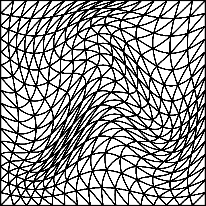
To test the scheme (47), we utilize an entropy conservative flux and run it on a uniform triangular mesh with a curvilinear warping shown in Figure 3. Theorem 2 ensures that, under an entropy conservative flux, (47) is semi-discretely entropy conservative. This does not hold at the fully discrete level; however, it is possible to verify that (47) is entropy stable using other approaches.
First, can examine the entropy RHS, which we define as the right hand side of (47) tested with
| (97) |
For positive density and pressure, (97) should be zero to machine precision. We can also track the change in entropy , which should converge to as the timestep approaches zero. Furthermore, the rate of convergence should match the order of the time-stepper used [59, 1].
Figure 4 shows the evolution of entropy over time , where the final time . We compare when the entropy-projected conservative variables are computed using the standard projection on the reference element, and when are computed using the weight-adjusted projection. For the standard projection, the change in entropy does not decrease as decreases (for a fixed mesh and order ). When is defined using the weight-adjusted projection, the entropy decreases as decreases. Moreover, the rate of convergence is approximately , which is slightly higher than the expected rate of when using LSRK-45. Regardless of whether the standard and weight-adjusted projection was used, the entropy RHS (97) is , indicating that the proposed scheme is implemented correctly.
These results suggest that the weight-adjusted projection is necessary to produce an entropy conservative scheme on curvilinear meshes. However, entropy conservative schemes result in spurious oscillations and lower convergence rates [1]. In practice, dissipative interface terms are added to produce entropy stable schemes. In the presence of interface dissipation, the evolution of entropy over time, errors for smooth solutions, and the qualitative behavior of the solution are very similar with or without the weight-adjusted projection. This may reflect the fact that aliasing-driven instabilities arise from the spatial discretization, and the entropy RHS (97) is machine precision zero with or without the weight-adjusted projection. In contrast, the presence of the weight-adjusted projection affects only the time-derivative on the left-hand side, and may not play as large a role in suppressing aliasing instabilities.
6.2.2. Local and global conservation
Next, we check that primary conservation is maintained numerically on curved meshes. We follow [15] and examine the semi-discrete evolution of the average of over the domain
| (98) |
The quantity (98) is computed using quadrature by multiplying the semi-discrete system (47) by
| (100) |
We consider three different cases:
-
(1)
Unmodified: the weight-adjusted DG scheme (47) is used without any special modifications,
- (2)
- (3)
All results use a Lax-Friedrichs flux, a CFL of , , and the curved mesh warping shown in Figure 3. We use volume quadrature rules from [55] which are exact for degree polynomials, and use -node 1D Gauss–Legendre quadrature rules on the faces.
Figure 5a shows computed conservation residuals from (100) on the curved mesh in Figure 3 for the discontinuous pulse initial condition (96). The conservation residual oscillates around for the unmodified scheme (47). Modifying the scheme using either the “Polynomial approximation” or “Conservative correction” approaches reduces the conservation error to between and . We have also studied the accuracy of each case in by comparing errors on a curved mesh for a smooth vortex solution at time . We observe that in all cases, the errors are virtually identical. For on an mesh, the errors for each case differ only in the 5th digit, while for the and meshes, they differ only in the 8th digit. This confirms that both approaches outlined in Section 4.3.1 restore primary conservation with no perceivable effect on accuracy.
6.2.3. Accuracy and convergence
Finally, we test the accuracy of the proposed schemes for smooth solutions on curved meshes in two dimensions. We use the isentropic vortex problem [60], which has an analytical solution
| (101) | ||||
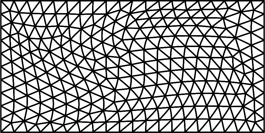
where are the and velocity and . Here, we take and . The solution is computed on a periodic rectangular domain at final time . Quasi-uniform triangular meshes are generated using GMSH [56], and a curvilinear warping is applied to the mesh to test the effect of non-affine mappings. This warping is shown in Figure 6 and is defined by mapping nodal positions on each triangle to warped nodal positions via
To ensure primary conservation, we use the “Polynomial Approximation” strategy described in Section 4.3.1 and compute the inverse of the weight-adjusted mass matrix using the degree projection instead of . The computed errors are shown in Figure 7. We observe optimal rates of convergence for . For degree , the rate of convergence is slightly higher than and may indicate that the mesh is not yet sufficiently fine for the error to show the asymptotic convergence rate.
6.3. Three dimensional compressible Euler equations
In three dimensions, the compressible Euler equations are given by
| (122) |
where the pressure and specific internal energy are defined
| (123) |
The formula for the entropy in three dimensions is the same as the two-dimensional formula (90). The entropy variables in three dimensions are
| (124) |
The conservation variables in terms of the entropy variables are given by
| (125) |
where and in terms of the entropy variables are
| (126) |
A set of entropy conservative numerical fluxes for the three-dimensional compressible Euler equations can be written as
| (137) | |||
| (143) |
where we have defined the auxiliary quantities
| (144) | ||||
6.3.1. Accuracy and convergence
As before, we test the accuracy of the proposed scheme using an isentropic vortex solution adapted to three dimensions. We take the solution to be the extruded 2D vortex propagating in the direction, whose analytic expression is derived from [61]
where is the velocity vector and
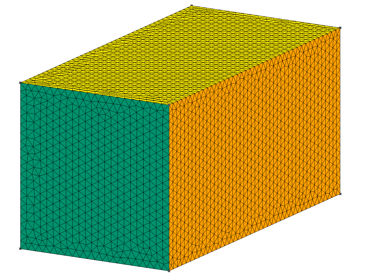
In this problem, we take , , and . The problem is solved on the domain . We use GMSH to construct three unstructured meshes consisting of 1354, 9543, and 72923 affine tetrahedra, corresponding to , , and (shown in Figure 8a). We apply a curvilinear warping by mapping nodal positions each tetrahedron to warped nodal positions via
The geometric terms are approximated using (83) to ensure the satisfaction of the discrete GCL. Figure 8 shows errors at final time for on both affine and curved meshes. In both cases, we observe optimal asymptotic rates of convergence for , while for we observe a rate which is slightly higher than but not quite . This may be due to the fact that the time-stepper is th order while the spatial discretization is th order.
We also compared approximations of geometric factors using degree polynomials via (83) and degree polynomials via (76). For the isentropic vortex problem on warped meshes, the approximation of the geometric factors does not impact accuracy significantly. Utilizing (76) and approximating geometric factors with degree polynomials only changed the error in the th significant digit, and resulted in the same asymptotic rates of convergence on curved 3D meshes. Future work will explore the effect of a more accurate geometric approximation on curved boundaries where a solid wall boundary condition is applied, where the approximation of geometry has been shown to have a more significant effect [62].
6.3.2. Inviscid Taylor–Green vortex
Our last numerical experiment investigates the behavior of entropy stable DG schemes for the inviscid Taylor–Green vortex [63, 35, 17]. The domain is the periodic box , and the initial conditions are given as
The Taylor–Green vortex is used to study the transition and decay of turbulence [64]. In the absence of viscosity, the Taylor–Green vortex develops smaller and smaller scales, implying that for sufficiently large times, the solution contains under-resolved features. We study the evolution of the kinetic energy
as well as the kinetic energy dissipation rate , which we approximate by differencing . Figure 9 shows the evolution of over time for both affine and curvilinear meshes with and . We also use a curved coarse mesh with element size test the convergence of the average entropy for a non-dissipative entropy conservative formulation as the timestep decreases. In both cases, the mesh is defined by constructing nodal positions from warpings of affine nodal positions as follows
The kinetic energy is plotted at 100 equally spaced times between . The simulation is stable and does not blow up despite the lack of filtering, limiting, or artificial viscosity. The results are qualitatively similar to those reported in the literature, with the kinetic energy dissipation rate increasing around and peaking with a value of roughly before [64, 35]. We also observe that, for an entropy conservative formulation, the average entropy appears to converge at a rate of for a 4th order time-stepping method. The same phenomena was also observed in [1, 17].
7. Conclusions
This work describes how to extend entropy conservative and entropy stable DG “modal” discretizations to curvilinear meshes using both weighted and weight-adjusted mass matrices. Assuming that the geometric terms satisfy a discrete geometric conservation law, the presented schemes allow for the use of over-integration while satisfying a semi-discrete entropy equality or inequality on curved meshes. Numerical results show the presented schemes achieve optimal rates of convergence for smooth solutions on both two and three dimensional affine and curvilinear meshes while remaining robust in the presence of under-resolved solutions such as shocks and turbulence.
Several outstanding computational questions remain to be answered. First, the use of weight-adjusted mass matrices is motivated by the low storage requirements and their efficient application on GPUs. However, to guarantee discrete entropy stability, the computation of a weight-adjusted projection is necessary, which adds additional computational cost compared to the affine case. Furthermore, numerical results suggest that, while computing the entropy-projected conservative variables using the weight-adjusted projection is necessary to ensure a semi-discrete conservation of entropy, the difference between using a weight-adjusted projection and regular projection may be negligible in practice. The necessity of the weight-adjusted projection in computing should be examined further. Secondly, on triangular and tetrahedral meshes, the proposed schemes involve more computational work than under-integrated collocation-style SBP schemes [19, 16, 17]. A careful computational comparison of the presented schemes with existing methods should be done to weigh the benefits of improved accuracy with additional computational costs.
Finally, we note that while this work has focused on triangular and tetrahedral elements, the approaches outlined here can be extended to more arbitrary pairings of (possibly non-polynomial) approximation spaces and quadratures. For example, similar techniques can be used to construct entropy stable B-spline or Galerkin difference discretizations on curved meshes [65, 39].
8. Acknowledgements
The authors thank Mark H. Carpenter and David C. Del Rey Fernandez for informative discussions. Jesse Chan is supported by NSF DMS-1719818 and DMS-1712639.
References
- [1] Jesse Chan. On discretely entropy conservative and entropy stable discontinuous Galerkin methods. Journal of Computational Physics, 362:346–374, June 2018. doi:10.1016/j.jcp.2018.02.033.
- [2] David A Kopriva. Metric identities and the discontinuous spectral element method on curvilinear meshes. Journal of Scientific Computing, 26(3):301–327, March 2006. doi:10.1007/s10915-005-9070-8.
- [3] Jesse Chan, Russell J Hewett, and T Warburton. Weight-adjusted discontinuous Galerkin methods: Wave propagation in heterogeneous media. SIAM Journal on Scientific Computing, 39(6):A2935–A2961, 2017. doi:10.1137/16m1089186.
- [4] Jesse Chan, Russell J Hewett, and T Warburton. Weight-adjusted discontinuous Galerkin methods: Curvilinear meshes. SIAM Journal on Scientific Computing, 39(6):A2395–A2421, 2017. doi:10.1137/16m1089198.
- [5] Fang Q Hu, MY Hussaini, and Patrick Rasetarinera. An analysis of the discontinuous Galerkin method for wave propagation problems. Journal of Computational Physics, 151(2):921–946, May 1999. doi:10.1006/jcph.1999.6227.
- [6] Mark Ainsworth. Dispersive and dissipative behaviour of high order discontinuous Galerkin finite element methods. Journal of Computational Physics, 198(1):106–130, July 2004. doi:10.1016/j.jcp.2004.01.004.
- [7] Zhijian J. Wang, Krzysztof Fidkowski, Rémi Abgrall, Francesco Bassi, Doru Caraeni, Andrew Cary, Herman Deconinck, Ralf Hartmann, Koen Hillewaert, Hung T Huynh, Norbert Kroll, Georg May, Per-Olof Persson, Bram van Leer, and Miguel Visbal. High-order CFD methods: Current status and perspective. International Journal for Numerical Methods in Fluids, 72(8):811–845, January 2013. doi:10.1002/fld.3767.
- [8] Per-Olof Persson and Jaime Peraire. Sub-cell shock capturing for discontinuous Galerkin methods. In 44th AIAA Aerospace Sciences Meeting and Exhibit. American Institute of Aeronautics and Astronautics, January 2006. doi:10.2514/6.2006-112.
- [9] Lilia Krivodonova. Limiters for high-order discontinuous Galerkin methods. Journal of Computational Physics, 226(1):879–896, September 2007. doi:10.1016/j.jcp.2007.05.011.
- [10] Garrett E Barter and David L Darmofal. Shock capturing with PDE-based artificial viscosity for DGFEM: Part I. Formulation. Journal of Computational Physics, 229(5):1810–1827, March 2010. doi:10.1016/j.jcp.2009.11.010.
- [11] Jean-Luc Guermond, Richard Pasquetti, and Bojan Popov. Entropy viscosity method for nonlinear conservation laws. Journal of Computational Physics, 230(11):4248–4267, May 2011. doi:10.1016/j.jcp.2010.11.043.
- [12] Travis C Fisher and Mark H Carpenter. High-order entropy stable finite difference schemes for nonlinear conservation laws: Finite domains. Journal of Computational Physics, 252:518–557, November 2013. doi:10.1016/j.jcp.2013.06.014.
- [13] Mark H Carpenter, Travis C Fisher, Eric J Nielsen, and Steven H Frankel. Entropy stable spectral collocation schemes for the Navier–Stokes equations: Discontinuous interfaces. SIAM Journal on Scientific Computing, 36(5):B835–B867, 2014. doi:10.1137/130932193.
- [14] Matteo Parsani, Mark H Carpenter, Travis C Fisher, and Eric J Nielsen. Entropy stable staggered grid discontinuous spectral collocation methods of any order for the compressible Navier–Stokes equations. SIAM Journal on Scientific Computing, 38(5):A3129–A3162, 2016. doi:10.1137/15m1043510.
- [15] Lucas Friedrich, Andrew R Winters, David C Del Rey Fernández, Gregor J Gassner, Matteo Parsani, and Mark H Carpenter. An entropy stable non-conforming discontinuous Galerkin method with the summation-by-parts property. arXiv preprint arXiv:1712.10234, 2017. URL: https://arxiv.org/abs/1712.10234.
- [16] Tianheng Chen and Chi-Wang Shu. Entropy stable high order discontinuous Galerkin methods with suitable quadrature rules for hyperbolic conservation laws. Journal of Computational Physics, 345:427–461, September 2017. doi:10.1016/j.jcp.2017.05.025.
- [17] Jared Crean, Jason E Hicken, David C Del Rey Fernández, David W Zingg, and Mark H Carpenter. Entropy-stable summation-by-parts discretization of the Euler equations on general curved elements. Journal of Computational Physics, 356:410–438, March 2018. doi:10.1016/j.jcp.2017.12.015.
- [18] Brian T Helenbrook. On the existence of explicit -finite element methods using Gauss–Lobatto integration on the triangle. SIAM Journal on Numerical Analysis, 47(2):1304–1318, 2009. doi:10.1137/070685439.
- [19] Jason E Hicken, David C Del Rey Fernández, and David W Zingg. Multidimensional summation-by-parts operators: General theory and application to simplex elements. SIAM Journal on Scientific Computing, 38(4):A1935–A1958, 2016. doi:10.1137/15m1038360.
- [20] PD Thomas and CK Lombard. Geometric conservation law and its application to flow computations on moving grids. AIAA Journal, 17(10):1030–1037, October 1979. doi:10.2514/3.61273.
- [21] Jesse Chan. Weight-adjusted discontinuous Galerkin methods: Matrix-valued weights and elastic wave propagation in heterogeneous media. International Journal for Numerical Methods in Engineering, 113(12):1779–1809, March 2018. doi:10.1002/nme.5720.
- [22] Thomas JR Hughes, LP Franca, and M Mallet. A new finite element formulation for computational fluid dynamics: I. symmetric forms of the compressible Euler and Navier-Stokes equations and the second law of thermodynamics. Computer Methods in Applied Mechanics and Engineering, 54(2):223–234, February 1986. doi:10.1016/0045-7825(86)90127-1.
- [23] Michael S Mock. Systems of conservation laws of mixed type. Journal of Differential Equations, 37(1):70–88, July 1980. doi:10.1016/0022-0396(80)90089-3.
- [24] Jesse Chan, Zheng Wang, Axel Modave, Jean-Francois Remacle, and T Warburton. GPU-accelerated discontinuous Galerkin methods on hybrid meshes. Journal of Computational Physics, 318:142–168, August 2016. doi:10.1016/j.jcp.2016.04.003.
- [25] Jan S Hesthaven and Tim Warburton. Nodal Discontinuous Galerkin Methods: Algorithms, Analysis, and Applications. Springer New York, 2008. doi:10.1007/978-0-387-72067-8.
- [26] Daniele Antonio Di Pietro and Alexandre Ern. Mathematical Aspects of Discontinuous Galerkin Methods. Springer Berlin Heidelberg, 2012. doi:10.1007/978-3-642-22980-0.
- [27] Bernardo Cockburn and Chi-Wang Shu. TVB Runge-Kutta local projection discontinuous Galerkin finite element method for conservation laws. II. General framework. Mathematics of Computation, 52(186):411–435, April 1989. doi:10.1090/s0025-5718-1989-0983311-4.
- [28] Bernardo Cockburn and Chi-Wang Shu. The Runge–Kutta discontinuous Galerkin method for conservation laws V: Multidimensional systems. Journal of Computational Physics, 141(2):199–224, April 1998. doi:10.1006/jcph.1998.5892.
- [29] Bernardo Cockburn. Devising discontinuous Galerkin methods for non-linear hyperbolic conservation laws. Journal of Computational and Applied Mathematics, 128(1-2):187–204, March 2001. doi:10.1016/s0377-0427(00)00512-4.
- [30] Jianxian Qiu, Boo Cheong Khoo, and Chi-Wang Shu. A numerical study for the performance of the Runge–Kutta discontinuous Galerkin method based on different numerical fluxes. Journal of Computational Physics, 212(2):540–565, March 2006. doi:10.1016/j.jcp.2005.07.011.
- [31] Xiangxiong Zhang, Yinhua Xia, and Chi-Wang Shu. Maximum-principle-satisfying and positivity-preserving high order discontinuous Galerkin schemes for conservation laws on triangular meshes. Journal of Scientific Computing, 50(1):29–62, January 2012. doi:10.1007/s10915-011-9472-8.
- [32] A Klöckner, T Warburton, and JS Hesthaven. Viscous shock capturing in a time-explicit discontinuous Galerkin method. Mathematical Modelling of Natural Phenomena, 6(3):57–83, 2011. doi:10.1051/mmnp/20116303.
- [33] Philippe G Ciarlet. The finite element method for elliptic problems. North-Holland Publishing Company, 1978.
- [34] Jan Nordström. Conservative finite difference formulations, variable coefficients, energy estimates and artificial dissipation. Journal of Scientific Computing, 29(3):375–404, December 2006. doi:10.1007/s10915-005-9013-4.
- [35] Gregor J Gassner, Andrew R Winters, and David A Kopriva. Split form nodal discontinuous Galerkin schemes with summation-by-parts property for the compressible Euler equations. Journal of Computational Physics, 327:39–66, December 2016. doi:10.1016/j.jcp.2016.09.013.
- [36] Roger A Horn and Charles R Johnson. Matrix Analysis. Cambridge University Press, 2nd edition, 2012.
- [37] Praveen Chandrashekar. Kinetic energy preserving and entropy stable finite volume schemes for compressible Euler and Navier-Stokes equations. Communications in Computational Physics, 14(5):1252–1286, November 2013. doi:10.4208/cicp.170712.010313a.
- [38] Andrew R Winters, Dominik Derigs, Gregor J Gassner, and Stefanie Walch. A uniquely defined entropy stable matrix dissipation operator for high Mach number ideal MHD and compressible Euler simulations. Journal of Computational Physics, 332:274–289, March 2017. doi:10.1016/j.jcp.2016.12.006.
- [39] Jesse Chan and John A Evans. Multi-patch discontinuous Galerkin isogeometric analysis for wave propagation: Explicit time-stepping and efficient mass matrix inversion. Computer Methods in Applied Mechanics and Engineering, 333:22–54, May 2018. doi:10.1016/j.cma.2018.01.022.
- [40] T Warburton. A low-storage curvilinear discontinuous Galerkin method for wave problems. SIAM Journal on Scientific Computing, 35(4):A1987–A2012, 2013. doi:10.1137/120899662.
- [41] Susanne C Brenner and L Ridgway Scott. The Mathematical Theory of Finite Element Methods. Springer New York, 3rd edition, 2008. doi:10.1007/978-0-387-75934-0.
- [42] Mo Lenoir. Optimal isoparametric finite elements and error estimates for domains involving curved boundaries. SIAM Journal on Numerical Analysis, 23(3):562–580, 1986. doi:10.1137/0723036.
- [43] Travis C Fisher, Mark H Carpenter, Jan Nordström, Nail K Yamaleev, and Charles Swanson. Discretely conservative finite-difference formulations for nonlinear conservation laws in split form: Theory and boundary conditions. Journal of Computational Physics, 234:353–375, February 2013. doi:10.1016/j.jcp.2012.09.026.
- [44] A Johnen, J-F Remacle, and C Geuzaine. Geometrical validity of curvilinear finite elements. Journal of Computational Physics, 233:359–372, January 2013. doi:10.1016/j.jcp.2012.08.051.
- [45] Miguel R Visbal and Datta V Gaitonde. On the use of higher-order finite-difference schemes on curvilinear and deforming meshes. Journal of Computational Physics, 181(1):155–185, September 2002. doi:10.1006/jcph.2002.7117.
- [46] Qi Chen and Ivo Babuška. The optimal symmetrical points for polynomial interpolation of real functions in the tetrahedron. Computer Methods in Applied Mechanics and Engineering, 137(1):89–94, October 1996. doi:10.1016/0045-7825(96)01051-1.
- [47] JS Hesthaven. From electrostatics to almost optimal nodal sets for polynomial interpolation in a simplex. SIAM Journal on Numerical Analysis, 35(2):655–676, 1998. doi:10.1137/s003614299630587x.
- [48] MG Blyth and C Pozrikidis. A Lobatto interpolation grid over the triangle. IMA Journal of Applied Mathematics, 71(1):153–169, February 2006. doi:10.1093/imamat/hxh077.
- [49] T Warburton. An explicit construction of interpolation nodes on the simplex. Journal of Engineering Mathematics, 56(3):247–262, November 2006. doi:10.1007/s10665-006-9086-6.
- [50] Jesse Chan and T Warburton. A comparison of high order interpolation nodes for the pyramid. SIAM Journal on Scientific Computing, 37(5):A2151–A2170, 2015. doi:10.1137/141000105.
- [51] DM Williams, Lee Shunn, and Antony Jameson. Symmetric quadrature rules for simplexes based on sphere close packed lattice arrangements. Journal of Computational and Applied Mathematics, 266:18–38, August 2014. doi:10.1016/j.cam.2014.01.007.
- [52] Freddie D Witherden and Peter E Vincent. On the identification of symmetric quadrature rules for finite element methods. Computers & Mathematics with Applications, 69(10):1232–1241, May 2015. doi:10.1016/j.camwa.2015.03.017.
- [53] David C Del Rey Fernández, Jason E Hicken, and David W Zingg. Simultaneous approximation terms for multi-dimensional summation-by-parts operators. Journal of Scientific Computing, 75(1):83–110, April 2018. doi:10.1007/s10915-017-0523-7.
- [54] Mark H Carpenter and Christopher A Kennedy. Fourth-order -storage Runge-Kutta schemes. Technical Report NASA-TM-109112, NAS 1.15:109112, NASA Langley Research Center, 1994. doi:2060/19940028444.
- [55] Hong Xiao and Zydrunas Gimbutas. A numerical algorithm for the construction of efficient quadrature rules in two and higher dimensions. Computers & Mathematics with Applications, 59(2):663–676, January 2010. doi:10.1016/j.camwa.2009.10.027.
- [56] Christophe Geuzaine and Jean-François Remacle. Gmsh: A 3-D finite element mesh generator with built-in pre- and post-processing facilities. International Journal for Numerical Methods in Engineering, 79(11):1309–1331, September 2009. doi:10.1002/nme.2579.
- [57] Florian Hindenlang, Gregor J Gassner, Christoph Altmann, Andrea Beck, Marc Staudenmaier, and Claus-Dieter Munz. Explicit discontinuous Galerkin methods for unsteady problems. Computers & Fluids, 61:86–93, May 2012. doi:10.1016/j.compfluid.2012.03.006.
- [58] Amiram Harten. On the symmetric form of systems of conservation laws with entropy. Journal of Computational Physics, 49(1):151–164, January 1983. doi:10.1016/0021-9991(83)90118-3.
- [59] Gregor J Gassner, Andrew R Winters, and David A Kopriva. A well balanced and entropy conservative discontinuous Galerkin spectral element method for the shallow water equations. Applied Mathematics and Computation, 272:291–308, January 2016. doi:10.1016/j.amc.2015.07.014.
- [60] Chi-Wang Shu. Essentially non-oscillatory and weighted essentially non-oscillatory schemes for hyperbolic conservation laws. In Advanced Numerical Approximation of Nonlinear Hyperbolic Equations, pages 325–432. Springer Berlin Heidelberg, 1998. doi:10.1007/bfb0096355.
- [61] David M Williams and Antony Jameson. Nodal points and the nonlinear stability of high-order methods for unsteady flow problems on tetrahedral meshes. In 21st AIAA Computational Fluid Dynamics Conference. American Institute of Aeronautics and Astronautics, June 2013. doi:10.2514/6.2013-2830.
- [62] Thomas Toulorge, Jonathan Lambrechts, and Jean-François Remacle. Optimizing the geometrical accuracy of curvilinear meshes. Journal of Computational Physics, 310:361–380, April 2016. doi:10.1016/j.jcp.2016.01.023.
- [63] Geoffrey I Taylor and Albert E Green. Mechanism of the production of small eddies from large ones. Proceedings of the Royal Society A: Mathematical, Physical and Engineering Sciences, 158(895):499–521, February 1937. doi:10.1098/rspa.1937.0036.
- [64] James DeBonis. Solutions of the Taylor-Green vortex problem using high-resolution explicit finite difference methods. In 51st AIAA Aerospace Sciences Meeting including the New Horizons Forum and Aerospace Exposition. American Institute of Aeronautics and Astronautics, January 2013. doi:10.2514/6.2013-382.
- [65] Jeffrey W Banks and Thomas Hagstrom. On Galerkin difference methods. Journal of Computational Physics, 313:310–327, 2016.