Exploring the generalized loosely bound Skyrme model

Abstract

The Skyrme model is extended with a sextic derivative term – called the BPS-Skyrme term – and a repulsive potential term – called the loosely bound potential. A large part of the model’s parameter space is studied for the 4-Skyrmion which corresponds to the Helium-4 nucleus and emphasis is put on preserving as much of the platonic symmetries as possible whilst reducing the binding energies. We reach classical binding energies for Helium-4 as low as $0.2\%$, while retaining the cubic symmetry of the 4-Skyrmion, and after taking into account the quantum mass correction to the nucleon due to spin/isospin quantization, we get total binding energies as low as $3.6\%$ – still with the cubic symmetry intact.

1 Introduction

The Skyrme model is an interesting approach to nuclear physics which is related to fundamental physics, i.e. it is a field theory Skyrme:1962vh ; Skyrme:1961vq ; indeed the soliton in the model is identified with the baryon in the large-$N$ limit of QCD Witten:1983tw ; Witten:1983tx . The soliton is called the Skyrmion. The most interesting aspect of the Skyrmions is that although a single Skyrmion is identified with a single nucleon, multi-Skyrmion solutions exist which can be identified with nuclei of higher baryon numbers. This fact distinguishes the Skyrme model from basically all other approaches to nuclear physics; the nuclei are no longer bound states of interacting point particles. What is more interesting is that since even the single Skyrmion is a spatially extended object (as opposed to a point particle), the multi-Skyrmions become extended objects with certain platonic symmetries Braaten:1989rg . A particular useful Ansatz for light nuclei was found using a rational map Houghton:1997kg . For larger nuclei, however, there is some consensus that when a pion mass term is included in the model, they are made of $B/4$ cubes – akin somewhat to the alpha particle model of nuclei Battye:2006na ; Feist:2012ps ; Lau:2014baa ; Halcrow:2016spb ; Rawlinson:2017rcq – up to small deformations.

A long standing problem of the Skyrme model as a model for nuclei is that the multi-Skyrmions are too strongly bound; their binding energies are about one order of magnitude larger than what is measured in nuclei experimentally. One approach to solving this problem is based on modifying the Skyrme model such that the classical solutions can come close to a BPS-like energy bound, in which case the classical energy is approximately proportional to the topological charge. Hence, if such a bound could be saturated, then classically the binding energy would vanish exactly. In the last decade, this approach has been taken in three different directions: the vector meson Skyrme model Sutcliffe:2010et ; Sutcliffe:2011ig ; Naya:2018mpt , the BPS-Skyrme model Adam:2010fg ; Adam:2010ds and the lightly/loosely bound Skyrme models Harland:2013rxa ; Gillard:2015eia ; Gudnason:2016mms .

The vector meson Skyrme model is inspired by approximate Skyrmion solutions obtained from instanton holonomies Atiyah:1992if and it is found that the instanton holonomy becomes an exact solution in the limit where an infinite tower of vector mesons is included; the complete theory can be described simply as a 4+1 dimensional Yang-Mills (YM) theory in flat spacetime Sutcliffe:2010et . The instanton is a half-BPS state in the YM theory and the Skyrmion saturates the BPS bound if the theory is not truncated. The standard Skyrme model is at the other end of the scale; all vector mesons have been stripped off, leaving behind just the pions. The model is in very close relation to holography, although the discrete spectrum of vector mesons is due to truncation of the theory and not due to an intrinsic curvature of the background spacetime Sutcliffe:2010et . Indeed in the Sakai-Sugimoto model, the standard Skyrme model comes out as the low-energy action of the zero modes Sakai:2004cn . The sextic term, which we shall discuss shortly in a different context, also comes out naturally by integrating out the first vector meson in the Sakai-Sugimoto model Bartolini:2017sxi .

The BPS-Skyrme model is based on a drastic modification of the Skyrme model: remove the original terms and replace them with a sextic term, which we shall call the BPS-Skyrme term, and a potential Adam:2010fg ; Adam:2010ds . The model has the advantage of simplicity in the following sense: the model in this limit is not only a BPS theory – in the sense of being able to saturate a BPS-like energy bound – but it is also integrable. That is, a large class of exact analytic solutions has been obtained. The disadvantage is that the kinetic term and the Skyrme term have to be quite suppressed in order for the classical binding energy to be of the order of magnitude seen in experimental data. That issue is two-fold; the first problem is that we would like to maintain the coefficient of the kinetic term (the pion decay constant) and pion mass of the order of the measured values in the pion vacuum. The second problem is of a more technical nature; close to the BPS limit, the coefficient of the kinetic term ($c_{2}$) is very small and hence there are certain points/lines in the Skyrmion solutions where the solution can afford to have very large field derivatives – of the order of $1/\sqrt{c_{2}}$. In ref. Gillard:2015eia the order of magnitude of $c_{2}$ for the classical binding energies to be in the ballpark of the experimental values was estimated to be around $c_{2}\sim 0.01$; whereas their numerics was trustable only down to about $c_{2}\sim 0.2$.

The lightly bound Skyrme model is based on an energy bound Harland:2013rxa ; Adam:2013tga for the Skyrme term and a potential to the fourth power. Although this model has a saturable solution in the 1-Skyrmion sector, no solutions saturate the bound for higher topological degrees. Nevertheless, it turns out that, although the solutions do not saturate the bound for higher topological degrees, they can come quite close to the bound, which in turn yields a small classical binding energy Gillard:2015eia . The lightly bound model can indeed reduce the binding energies, but it comes with a price; long before realistic binding energies are reached, the platonic symmetries of the compact Skyrmions are lost and the potential has the effect of pushing out identifiable 1-Skyrmions which remain only very weakly bound. This limit was the inspiration for a simplified kind of Skyrme model, called the point particle model of lightly bound Skyrmions Gillard:2016esy . Said limit can also be obtained naturally in the Sakai-Sugimoto model by considering the strong ’t Hooft coupling limit Baldino:2017mqq .

In ref. Gudnason:2016mms , we compared the potential made of the standard pion mass term to the fourth power and the same potential to the second power; we call them the lightly bound and the loosely bound potentials, respectively. It turns out that the loosely bound potential has the same repulsive effect as the lightly bound potential does, but the Skyrmions retain their platonic symmetries down to smaller binding energies for the loosely bound potential as compared to the lightly bound one. In ref. Gudnason:2016cdo , we further established that if the potential is treated as a polynomial in $\sigma=\tfrac{1}{2}{\rm Tr}\,[U]$, where $U$ is the chiral field, then to second order, the loosely bound potential is the potential that can reduce the binding energy the most while preserving platonic symmetries of the Skyrmions.

In ref. Gudnason:2016tiz , we expanded the model by making a hybrid model out of the BPS-Skyrme-type models and the loosely bound model. Let us define the generalized Skyrme model as the standard Skyrme model with the addition of the sextic BPS-Skyrme term. Thus in ref. Gudnason:2016tiz we studied the generalized Skyrme model with the pion mass term and the loosely bound potential. More precisely, we studied the model using the rational map Ansatz for the 4-Skyrmion in the regime where the coefficients for the BPS-Skyrme term, $c_{6}$, and the loosely bound potential, $m_{2}$, were both taken to be small (i.e. smaller or equal to one). Physical effects on the observables of the model could readily be extracted without the effort of full numerical PDE (partial differential equation) calculations. Of course, that compromise had the consequence that we could not detect the change of symmetry in the Skyrmion solutions and hence we investigated only a very restricted part of the parameter space.

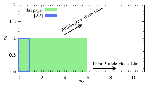
Figure 1: Parameter space of the model explored in this paper (green) as well as what was studied in ref. Gudnason:2016tiz (region inside the blue box). The BPS-Skyrme Model Limit (BSML) is defined as $c_{6}\propto m_{2}\to\infty$ and the Point Particle Model Limit (PPML) is $c_{6}=0$, $m_{2}\to\infty$.

In this paper, we perform the full PDE calculations for the 4-Skyrmion in the generalized Skyrme model with the loosely bound potential and a standard pion mass term, for small values of the coefficient of the BPS-Skyrme term and up to large values of the mass parameter of the loosely bound potential, see fig. 1. In particular, in this paper we study the following region of parameter space: $c_{6}\in[0,1]$ and $m_{2}\in[0,6]$. Note that it is $m_{2}^{2}$ that enters the Lagrangian and hence $6^{2}=36$ is much larger than the other coefficients in the Lagrangian (which are all of order one). In fact, we are close to the limit of how far we can push $m_{2}$ with the current numerical codes. We have not considered the direction of large $c_{6}$ in this work, as it will not reduce the binding energy unless we also turn on a large coefficient of the potential. That situation, however, yields two possibilities: either we do not go beyond the limit where the numerics becomes difficult as discussed above, or one has to take the near-BPS limit carefully, which will require overcoming further technical obstacles than dealt with here. Nevertheless, in the part of parameter space we have studied in this paper, we are able to obtain a classical binding energy of the 4-Skyrmion as low as $0.2\%$ – about a factor of four smaller than the experimental value for Helium-4. After taking into account the quantum correction to the mass of the nucleon due to the spin contribution (as it is a spin-$\tfrac{1}{2}$ state in the ground state), the binding energy increases to about $3.6\%$ – about a factor of $4.5$ too large. This fact suggests that we cannot leave out further quantum corrections to the nuclear masses; we have to take into account quantum corrections due to massive modes Barnes:1997gv , also called vibrational modes, see e.g. refs. Halcrow:2015rvz ; Halcrow:2016spb ; Gudnason:2018aej .

The question remains how large a total contribution the inclusion of the quantum corrections due to the massive modes will give. It has been assumed all along that the quantization of solitons can consistently be made in a semi-classical fashion, where the quantum corrections are small compared to the (large) mass scale of the soliton. This expectation is based on the assumption that the fluctuation spectrum is weakly coupled, even though the soliton is inherently a non-perturbative object. The simplest example is to consider the mass correction to the kink in the $\lambda\phi^{4}$ model in 1+1 dimensions

$$\mathcal{L}^{\rm kink}=-\frac{1}{2}(\partial_{\mu}\phi)^{2}-\frac{\lambda}{4\hbar^{3}}\left(\phi^{2}-\frac{\hbar m^{2}}{\lambda}\right)^{2}.$$ (1)

We can estimate the kink mass with the following back-of-an-envelope estimate: we rescale the length scale $x^{\mu}\to\hbar x^{\mu}/m$ and rescale the field $\phi\to\sqrt{\frac{\hbar}{\lambda}}m\phi$; the Lagrangian density is now dimensionless with an overall dimensionful prefactor of $\frac{m^{4}}{\hbar\lambda}$. Assuming the kink exists, its mass must be an order one number times $\frac{m^{3}}{\lambda}$ where the $\hbar/m$ came from integrating over $x^{1}$. Considering now the quantum correction due to massive modes, one obtains an order-one number times $\hbar\omega$, where $\omega^{2}$ is the curvature of the effective potential created by the kink solution Dashen:1974cj . That is, the eigenvalue of the fluctuation around the kink is $\omega^{2}\sim m^{2}/\hbar^{2}$ and it follows in the harmonic approximation that the quantum energy is $\hbar\omega\sim m$. To realize this, it suffices to note that the second variation of the potential with respect to the field is $-\frac{m^{2}}{\hbar^{2}}+3\frac{\lambda}{\hbar^{3}}\phi_{\rm soliton}^{2}$ and that the soliton solution is proportional to $\hbar^{\frac{1}{2}}\lambda^{-\frac{1}{2}}m$; the resultant effective potential for the fluctuations is thus independent of $\lambda$. In this example the mass dimensions of $m$ and $\lambda$ are 1 and 2, respectively. If $\lambda\ll m^{2}$ then the perturbation series makes sense and furthermore, the quantum correction is much smaller than the classical contribution

$$M_{\rm classical}+\delta M\propto\frac{m^{3}}{\lambda}\left(1+\mathcal{O}\left(\frac{\lambda}{m^{2}}\right)\right).$$ (2)

The situation is more complicated in the case of the 3-dimensional Skyrmions than in the case of simple 1-dimensional kinks (which are integrable). First of all, it is not known to the best of the author’s knowledge, how weakly coupled the fluctuation spectrum really is. Comparing to the kinks, the question would be how small $\lambda^{\rm eff}$ is for the Skyrmions.

The scope in this paper, however, will be to focus on reducing the classical binding energy of the Skyrmions under the constraint of preserving as much symmetry of the original Skyrmions as possible. This is thus in the spirit of assuming that the fluctuation spectrum of the Skyrmions is weakly coupled and thus the classical mass is the largest contribution to the mass by far; the zero-mode quantization gives the most important quantum corrections and the remaining modes give corrections to the mass of the order of magnitude of the zero-mode contributions or less. The reason for preserving as much symmetry as possible is first of all to be able to keep some of the phenomenological successes of the Skyrme model already obtained; such as the Hoyle state and its corresponding rotational band having a slope a factor of 2.5 lower than that of the ground state Lau:2014baa . Taking into account the vibrational spectrum of the 4-Skyrmions vibrating between a flat square configuration and a tetrahedral arrangement was crucial in obtaining the right spectrum of Oxygen-16, having a large energy splitting between states of the same spins and opposite parity Halcrow:2016spb . Both of these results would fall apart if the 4-Skyrmion loses its cubic symmetry. Finally, and perhaps even more importantly, the larger the symmetry, the better the chances are that the symmetry can eliminate unwanted degeneracies, e.g. the parity doubling found in the $B=5$ cluster system in the model of ref. Gudnason:2018aej .

The paper is organized as follows. In the next section we will introduce the model, define the observables and finally propose an order parameter for a quantitative measure of the symmetry change. In sec. 3 we will present the numerical results. Finally, sec. 4 concludes the paper with a discussion of the results and what to do next.

2 The model

The model we study in this paper is the generalized Skyrme model – consisting of a kinetic term, the Skyrme term and the BPS-Skyrme term – with a pion mass term and the so-called loosely bound potential. In physical units we have

$$\mathcal{L}=\frac{\tilde{f}_{\pi}^{2}}{4}\mathcal{L}_{2}+\frac{1}{e^{2}}\mathcal{L}_{4}+\frac{4c_{2}c_{6}}{c_{4}^{2}e^{4}\tilde{f}_{\pi}^{2}}\mathcal{L}_{6}-\frac{\tilde{m}_{\pi}^{2}\tilde{f}_{\pi}^{2}}{4m_{1}^{2}}V,$$ (3)

where the kinetic term, the Skyrme term Skyrme:1962vh ; Skyrme:1961vq and the BPS-Skyrme term Adam:2010fg ; Adam:2010ds are given by

$$\mathcal{L}_{2} =\frac{1}{4}{\rm Tr}\,(L_{\mu}L^{\mu}),$$ (4)

$$\mathcal{L}_{4} =\frac{1}{32}{\rm Tr}\,([L_{\mu},L_{\nu}][L^{\mu},L^{\nu}]),$$ (5)

$$\mathcal{L}_{6} =\frac{1}{144}\eta_{\mu\mu^{\prime}}(\epsilon^{\mu\nu\rho\sigma}{\rm Tr}\,[L_{\nu}L_{\rho}L_{\sigma}])(\epsilon^{\mu^{\prime}\nu^{\prime}\rho^{\prime}\sigma^{\prime}}{\rm Tr}\,[L_{\nu^{\prime}}L_{\rho^{\prime}}L_{\sigma^{\prime}}]),$$ (6)

with the left-invariant current defined as

$$L_{\mu}\equiv U^{\dagger}\partial_{\mu}U,$$ (7)

in terms of the chiral Lagrangian or Skyrme field $U$ which is related to the pions as

$$U=\mathbf{1}_{2}\sigma+i\boldsymbol{\tau}\cdot\boldsymbol{\pi},$$ (8)

with the nonlinear sigma model constraint $\det U=1$ or $\sigma^{2}+\boldsymbol{\pi}\cdot\boldsymbol{\pi}=1$ and $\boldsymbol{\tau}$ is a 3-vector of the Pauli matrices. The Greek indices $\mu,\nu,\rho,\sigma=0,1,2,3$ denote spacetime indices and we will use the mostly positive metric signature throughout the paper.

We will now switch to (dimensionless) Skyrme units following ref. Gudnason:2016cdo ; Gudnason:2016tiz and denote the quantities having physical units with a tilde. In particular, for the energy and length scale we will take $\tilde{E}=\tilde{\lambda}E$ and $\tilde{x}^{i}=\tilde{\mu}x^{i}$, respectively, where we have the units Gudnason:2016tiz

$$\tilde{\lambda}=\frac{\tilde{f}_{\pi}}{2e\sqrt{c_{2}c_{4}}},\qquad\tilde{\mu}=\sqrt{\frac{c_{2}}{c_{4}}}\frac{2}{e\tilde{f}_{\pi}},$$ (9)

and finally the pion mass in physical units Gudnason:2016tiz

$$\tilde{m}_{\pi}=\frac{\sqrt{c_{4}}}{2c_{2}}e\tilde{f}_{\pi}m_{1}.$$ (10)

Hence in dimensionless units, the Lagrangian (3) reads

$$\mathcal{L}=c_{2}\mathcal{L}_{2}+c_{4}\mathcal{L}_{4}+c_{6}\mathcal{L}-V.$$ (11)

For a positive definite energy density, we require $c_{2}>0$, $c_{4}>0$ and $c_{6}\geq 0$.

The potential we will consider in this paper is due to the results of ref. Gudnason:2016mms , which showed that the pion mass term squared lowers the binding energy further than the pion mass term to the fourth power while keeping the symmetries of the 4-Skyrmion. We will also include the standard pion mass term and thus the total potential is

$$V=V_{1}+V_{2},$$ (12)

where we have defined

$$V_{n}\equiv\frac{1}{n}m_{n}^{2}(1-\sigma)^{n},$$ (13)

and $\sigma=\tfrac{1}{2}{\rm Tr}\,[U]$. Only $V_{1}$ gives a contribution to the pion mass. Both $V_{1}$ and $V_{2}$ break explicitly the chiral symmetry SU(2)${}_{\rm L}\times$SU(2)_R to the diagonal SU(2)_L+R. The target space is thus SU(2)${}_{\rm L}\times$SU(2)${}_{\rm R}/$SU(2)${}_{\rm L+R}\simeq$ SU(2) $\simeq S^{3}$. Since the Skyrmion, which is identified with the baryon, is a texture Vilenkin:2000 , it is characterized by the topological degree, $B$,

$$\pi_{3}(S^{3})=\mathbb{Z}\ni B,$$ (14)

where $B$ is called the baryon number. The baryon number or topological degree of a Skyrmion configuration can be calculated by

$$B=\frac{1}{2\pi^{2}}\int d^{3}x\;\mathcal{B}^{0},\qquad\mathcal{B}^{\mu}=-\frac{1}{12}\epsilon^{\mu\nu\rho\sigma}{\rm Tr}\,(L_{\nu}L_{\rho}L_{\sigma}).$$ (15)

We will throughout the paper denote Skyrmions of degree $B$ as $B$-Skyrmions.

Finally, for the numerical calculations we have to settle on a choice of normalization of the units and we follow that of refs. Gudnason:2016mms ; Gudnason:2016cdo ; Gudnason:2016tiz ,

$$c_{2}=\frac{1}{4},\qquad c_{4}=1,$$ (16)

and hence the energies and lengths are given in units of $\tilde{f}_{\pi}/e$ and $1/(e\tilde{f}_{\pi})$, respectively, while the physical pion mass is given by

$$\tilde{m}_{\pi}=\frac{\sqrt{c_{4}}}{2c_{2}}e\tilde{f}_{\pi}\left.\sqrt{-\frac{\partial V}{\partial\sigma}}\right|_{\sigma=1}=2e\tilde{f}_{\pi}m_{1},$$ (17)

where we have used the coefficients (16). In this paper we will use $m_{1}=1/4$ Gudnason:2016mms .

2.1 Observables

In this section we will list the observables to be measured in the numerical calculations. Since they are greatly overlapping with our previous studies, we will only review them briefly here and refer to ref. Gudnason:2016tiz for details. As in refs. Gudnason:2016cdo ; Gudnason:2016tiz we will only consider the 4-Skyrmion in this paper, as it plays a unique role in the alpha-particle interpretation of the Skyrme model and it is the building block of the lattice structure appearing for large nuclei Battye:2006na ; Feist:2012ps ; Lau:2014baa ; Halcrow:2016spb ; Rawlinson:2017rcq . More importantly, it is where to look for the change in symmetry that inevitably kicks in for strongly repulsive potentials, see e.g. the point particle model Gillard:2015eia ; Gillard:2016esy and also ref. Gudnason:2016mms .

As usual we are interested in the classical and spin/isospin quantum-corrected binding energies. The energy of the 1-Skyrmion is obtained by minimizing the static energy corresponding to (minus) the Lagrangian (11) for the hedgehog

$$U=\mathbf{1}_{2}\cos f(r)+i\hat{\mathbf{x}}\cdot\boldsymbol{\tau}\sin f(r),$$ (18)

where $\hat{\mathbf{x}}\equiv{\mathbf{x}}/r$ is the unit 3-vector at the origin and $r=\sqrt{\mathbf{x}\cdot\mathbf{x}}$ is the radial coordinate. We will call the energy of the $B$-Skyrmion $E_{B}$. As the initial condition for the 4-Skyrmion, we will use the rational map Ansatz Houghton:1997kg

$$U =\mathbf{1}_{2}\cos f(r)+i\mathbf{n}_{R}\cdot\boldsymbol{\tau}\sin f(r),$$ (19)

$$\mathbf{n}_{R} =\left(\frac{R+\bar{R}}{1+|R|^{2}},\frac{i(\bar{R}-R)}{1+|R|^{2}},\frac{1-|R|^{2}}{1+|R|^{2}}\right),$$ (20)

$$R(z) =\frac{z^{4}+2\sqrt{3}iz^{2}+1}{z^{4}-2\sqrt{3}iz^{2}+1},$$ (21)

for the $c_{6}=0$, $m_{2}=0$ solution and $z=e^{i\phi}\tan(\tfrac{\theta}{2})$ is the Riemann sphere coordinate. Once a numerical solution has been obtained, we can calculate the classical relative binding energy (CRBE) of the 4-Skyrmion as

$$\delta_{4}=1-\frac{E_{4}}{4E_{1}},$$ (22)

and the quantum-corrected relative binding energy (QRBE) as

$$\delta_{4}^{\rm tot}=1-\frac{E_{4}}{4(E_{1}+\epsilon_{1})},$$ (23)

where $\epsilon_{1}$ is the quantum correction due to the isospin quantization of the 1-Skyrmion. The CRBE (22) is independent of the physical units and thus independent of the calibration of the model. The QRBE (23), on the other hand, after factoring out the energy units, still depends on the Skyrme coupling $e$.

Calibrating the Skyrme-like models can be done in many ways and often ways are invented to minimize the problem of over-binding by compensating with a better calibration. In this paper, we will not turn to the calibration for compensating the over-binding, but try to reduce the binding energy by varying the parameters of the Lagrangian (11). Thus, we will stick with a simple calibration where we set the mass and size of the 4-Skyrmion to those of Helium-4. In order to calculate the electric charge radius of the 4-Skyrmion, we note that the ground state of Helium-4 is an isospin 0 state and thus the charge radius in the Skyrme model is given entirely by the baryon charge radius Gudnason:2016tiz

$$r_{4}^{2}=r_{4,E}^{2}=r_{4,B}^{2}=\frac{1}{8\pi^{2}}\int d^{3}x\;r^{2}\mathcal{B}^{0}.$$ (24)

The calibration now reads Gudnason:2016tiz

$$\tilde{f}_{\pi}=2\sqrt{c_{2}}\sqrt{\frac{r_{4}\tilde{M}_{{}^{4}{\rm He}}}{\tilde{r}_{{}^{4}{\rm He}}E_{4}}}=\sqrt{\frac{r_{4}\tilde{M}_{{}^{4}{\rm He}}}{\tilde{r}_{{}^{4}{\rm He}}E_{4}}},\qquad e=\frac{1}{\sqrt{c_{4}}}\sqrt{\frac{r_{4}E_{4}}{\tilde{r}_{{}^{4}{\rm He}}\tilde{M}_{{}^{4}{\rm He}}}}=\sqrt{\frac{r_{4}E_{4}}{\tilde{r}_{{}^{4}{\rm He}}\tilde{M}_{{}^{4}{\rm He}}}},$$ (25)

where in the latter expressions, we plugged in the normalization (16) and the experimental data used here are $\tilde{M}_{{}^{4}{\rm He}}=3727\;{\rm MeV}$ and $\tilde{r}_{{}^{4}{\rm He}}=8.492\times 10^{-3}\;{\rm MeV}^{-1}$.

With the calibration in place, we can now determine the quantum correction to the mass of the 1-Skyrmion due to (spin/)isospin quantization (with the normalization (16))

$$\tilde{m}_{N}\equiv\tilde{M}_{1}=\frac{\tilde{f}_{\pi}}{e}\left(E_{1}+\epsilon_{1}\right)=\tilde{E}_{1}+\tilde{\epsilon}_{1},\qquad\epsilon_{1}=\frac{e^{4}}{2\Lambda}J(J+1),$$ (26)

where $\Lambda$ is the diagonal component of the isospin inertia tensor for the 1-Skyrmion: $U_{ij}=\Lambda\delta^{ij}$ where $U_{ij}$ is given in the next section in eq. (33). For the hedgehog Ansatz (18) the expression for $\Lambda$ reads

$$\Lambda=\frac{8\pi}{3}\int dr\;r^{2}\sin^{2}f\left(c_{2}+c_{4}f_{r}^{2}+\frac{c_{4}}{r^{2}}\sin^{2}f+\frac{2c_{6}\sin^{2}(f)f_{r}^{2}}{r^{2}}\right).$$ (27)

Finally, for the ground state of the proton, $J=\tfrac{1}{2}$ and thus $\epsilon_{1}=\frac{3e^{4}}{8\Lambda}$. We will also consider the $\Delta$ resonance as a spin-$\tfrac{3}{2}$ excitation of the 1-Skyrmion Adkins:1983ya yielding

$$\tilde{m}_{\Delta}=\frac{\tilde{f}_{\pi}}{e}\left(E_{1}+5\epsilon_{1}\right).$$ (28)

The $\Delta$ resonance is nevertheless problematic in the Skyrme model, see the discussion.

As the ground state of Helium-4 is a spin-0, isospin-0 state, there is no quantum correction to the mass due to zero-mode quantization (although there are corrections due to massive modes, see the discussion).

Finally, we will consider the electric charge radius of the proton and the axial coupling. The details and tensor expressions are given in ref. Gudnason:2016tiz and we will just state the final results here

$$r_{1,E}^{2} =\frac{1}{2}r_{1,B}^{2}+\frac{\int dr\;r^{2}\left(c_{2}r^{2}\sin^{2}f+c_{4}\sin^{2}(f)\left(\sin^{2}f+r^{2}f_{r}^{2}\right)+2c_{6}\sin^{4}(f)f_{r}^{2}\right)}{2\int dr\;\left(c_{2}r^{2}\sin^{2}f+c_{4}\sin^{2}(f)\left(\sin^{2}f+r^{2}f_{r}^{2}\right)+2c_{6}\sin^{4}(f)f_{r}^{2}\right)},$$ (29)

$$g_{A} =-\frac{4\pi}{3}\int dr\;r\bigg{[}c_{2}(\sin 2f+rf_{r})+c_{4}\left(\frac{\sin^{2}f\sin 2f}{r^{2}}+\frac{2\sin^{2}(f)f_{r}}{r}+\sin(2f)f_{r}^{2}\right)$$

$$\phantom{=-\frac{4\pi}{3}\int dr\;r\bigg{[}}+\frac{2c_{6}\sin^{2}f}{r^{2}}\left(\frac{\sin^{2}(f)f_{r}}{r}+\sin(2f)f_{r}^{2}\right)\bigg{]},$$ (30)

where the baryon charge radius is

$$r_{1,B}^{2}=-\frac{2}{\pi}\int dr\;r^{2}\sin^{2}(f)f_{r},$$ (31)

and the axial coupling in physical units is given by

$$\tilde{g}_{A}=\frac{g_{A}}{c_{4}e^{2}}=\frac{g_{A}}{e^{2}},$$ (32)

which is obtained by multiplying the dimensionless expression by $\tilde{\lambda}\tilde{\mu}$ and in the last expression we have used the normalization (16).

Some geometric observables that we will calculate, are the tensors of inertia corresponding to the spin and the isospin of the 4-Skyrmion. For the generalized model (3) they can be written as

$$U_{ij} =-\frac{1}{2}\int d^{3}x\;\Big{(}c_{2}{\rm Tr}\,(T_{i}T_{j})+\frac{c_{4}}{4}{\rm Tr}\,([L_{k},T_{i}][L_{k},T_{j}])-\frac{c_{6}}{8}{\rm Tr}\,(T_{i}[L_{k},L_{l}]){\rm Tr}\,(T_{j}[L_{k},L_{l}])\Big{)},$$ (33)

$$V_{ij} =-\frac{1}{2}\int d^{3}x\;\epsilon^{imn}\epsilon^{jpq}x^{m}x^{p}\Big{(}c_{2}{\rm Tr}\,(L_{n}L_{q})+\frac{c_{4}}{4}{\rm Tr}\,([L_{k},L_{n}][L_{k},L_{q}])$$

$$\phantom{=-\frac{1}{2}\int d^{3}x\;\epsilon^{imn}\epsilon^{jpq}x^{m}x^{p}\Big{(}}-\frac{c_{6}}{8}{\rm Tr}\,(L_{n}[L_{k},L_{l}]){\rm Tr}\,(L_{q}[L_{k},L_{l}])\Big{)},$$ (34)

$$W_{ij} =\frac{1}{2}\int d^{3}x\;\epsilon^{jmn}x^{m}\Big{(}c_{2}{\rm Tr}\,(T_{i}L_{n})+\frac{c_{4}}{4}{\rm Tr}\,([L_{k},T_{i}][L_{k},L_{n}])$$

$$\phantom{=-\frac{1}{2}\int d^{3}x\;\epsilon^{jmn}x^{m}\Big{(}}-\frac{c_{6}}{8}{\rm Tr}\,(T_{i}[L_{k},L_{l}]){\rm Tr}\,(L_{n}[L_{k},L_{l}])\Big{)},$$ (35)

and they enter the kinetic energy of the Lagrangian (11) as

$$\mathcal{T}=\frac{1}{2}a_{i}U_{ij}a_{j}-a_{i}W_{ij}b_{j}+\frac{1}{2}b_{i}V_{ij}b_{j},$$ (36)

where the isospin and spin angular momenta, respectively, are defined as

$$a_{i}\equiv-i{\rm Tr}\,[\tau_{i}A^{-1}\dot{A}],\qquad b_{i}\equiv i{\rm Tr}\,[\tau_{i}\dot{B}B^{-1}],$$ (37)

and they act on the static Skyrme field, $U_{0}(x^{i})$, as

$$U=AU_{0}(R^{i}_{\phantom{i}j}x^{j})A^{-1},\qquad R^{i}_{\phantom{i}j}={\rm Tr}\,[\tau^{i}B\tau_{j}B^{-1}],$$ (38)

where $B(t)$ ($A(t)$) is an SU(2) matrix that transforms the static Skyrmion to the (iso)spinning Skyrmion.

2.2 Symmetry

One could contemplate how to extract the symmetries from a numerical Skyrmion configuration. One guess could be to use the tensors of inertia which encode geometrical information about the soliton, in particular related to its spinning and isospinning. Another more brute-force attempt could be to take moments of the energy; schematically $\int(x^{1})^{n_{1}}(x^{2})^{n_{2}}(x^{3})^{n_{3}}\mathcal{E}$. This, in principle, could extract further geometrical information from the numerical Skyrmion.

However, we are interested in a particular symmetry, namely octahedral symmetry and would like to know when it is broken to its tetrahedral subgroup. Therefore we can use the transformations of the octahedral symmetry which are not symmetry transformations of the tetrahedral subgroup. In the following, we place a cube such that the Cartesian axes are perpendicular to 3 of its faces and the origin is at the center of the cube. The tetrahedral symmetry group contains the following transformations: the identity, three $C_{2}$ transformations and eight $C_{3}$ transformations. The $C_{2}$ transformations rotate the cube by $\pi$ around one of the Cartesian axes and the $C_{3}$ transformations rotate the cube by $\pm 2\pi/3$ around an axis in the $(1,1,1)$, $(-1,-1,1)$, $(1,-1,-1)$ or $(-1,1,-1)$ direction. The octahedral symmetry group includes another six $C_{2}$ transformations as well as three $C_{4}$ transformations. The $C_{2}$ transformations rotate the cube by $\pi$ in the $(1,1,0)$, $(-1,1,0)$, $(1,0,1)$, $(1,0,-1)$, $(0,-1,1)$ or $(0,-1,-1)$ direction and the $C_{4}$ transformations rotate the cube by $\pi/2$ around one of the Cartesian axes. We should choose a transformation among the latter two, which only resides in the octahedral symmetry group and is lost when only a tetrahedral subgroup of the symmetry is preserved.

We choose to construct an order parameter for the octahedral symmetry as follows. Let us choose one of the $C_{4}$ symmetry transformations, say about the $x$-axis. The meaning of the Skyrmion possessing such a discrete symmetry is of course that after rotating the Skyrmion by $\pi/2$ about the $x$-axis, we must subsequently perform an appropriate rotation in isospin space to get back to the original Skyrmion. The appropriate isospin rotation to follow the (spatial) $C_{4,x}$ rotation is a rotation by $\pi$ in isospin space about the $\pi_{1}$-axis. The 4-Skyrmion possessing octahedral symmetry will be invariant under these two subsequent transformations, while the tetrahedrally symmetric 4-Skyrmion will not. We can thus construct the order parameter for octahedral symmetry as follows. We perform the $C_{4}$ transformation as well as the $C_{2}$ transformation in isospin space on the Skyrmion and then subtract off the original Skyrmion, take a 2-norm of the resulting field and finally integrate over space. If the symmetry is preserved, this integral vanishes. We thus define

$$\sigma^{O_{h}}\equiv\frac{1}{V}\int d^{3}x\;{\rm Tr}\,\left[\left(\left(e^{i\pi\hat{I}_{1}}e^{\frac{i\pi}{2}\hat{J}_{1}}-1\right)U\right)^{\dagger}\left(e^{i\pi\hat{I}_{1}}e^{\frac{i\pi}{2}\hat{J}_{1}}-1\right)U\right],$$ (39)

where we have divided by the volume of the Skyrmion, $V\equiv\frac{4}{3}\pi r_{4}^{3}$, in order to get a dimensionless result.

With all observables at hand we are now ready to turn to the numerical calculations.

3 Numerical results

The numerical calculations in this paper are all carried out on cubic lattices of size $121^{3}$ with a spatial lattice constant of about $h_{x}=0.08$ and the derivatives are approximated by a finite difference method using a fourth-order stencil. In previous works we were able to use the relaxation method with a forward-time algorithm, but that turns out to be too slow for the generalized Skyrme model when including the BPS-Skyrme term (with nonvanishing $c_{6}$). In this paper, therefore, we used the method of nonlinear conjugate gradients to find the numerical solutions. Although standard implementations of the algorithm work smoothly for small values of the potential parameter $m_{2}\lesssim 1$, some nontrivial tweaking and a sophisticated line search algorithm was needed for ensuring convergence in the large-$m_{2}$ part of the parameter space. In particular, we found a viable solution based on switching between the Newton-Raphson algorithm and a line search using a quadratic fit along the search direction of the conjugate gradients method.

As a handle on the precision we checked that the numerically integrated baryon charge is captured by the solution to within $0.15\%$. In addition to this, we stopped the algorithm when a local precision of the equation of motion better than $1.7\times 10^{-6}$ was obtained.

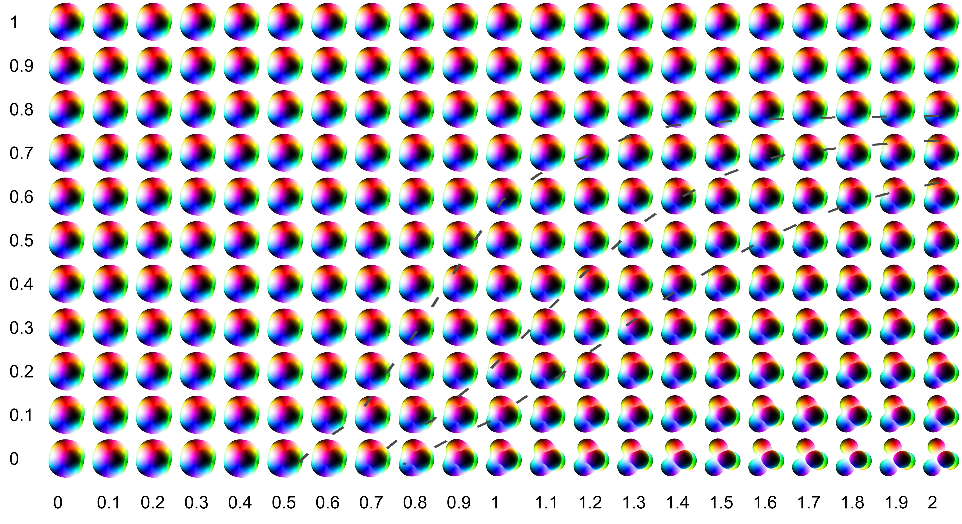
Figure 11: Baryon charge density isosurfaces of the 4-Skyrmion solutions over part of the scanned parameter space. The vertical axis denotes the values of $c_{6}$ while the horizontal axis is $m_{2}$. The dashed lines show contours of $\sigma^{O_{h}}=0.1,0.5,1$ from top to bottom. The center of mass of the Skyrmion corresponds to its position in parameter space.

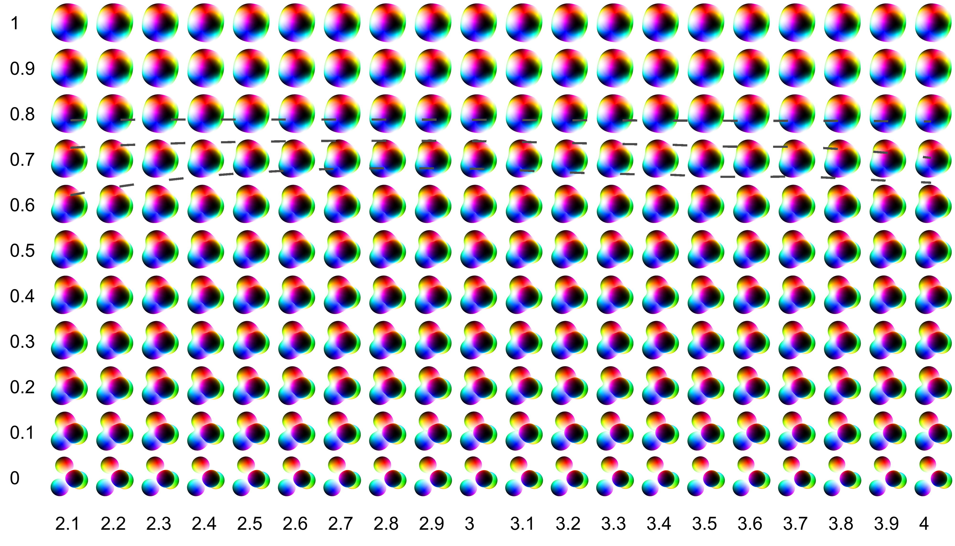
Figure 12: Baryon charge density isosurfaces of the 4-Skyrmion solutions over part of the scanned parameter space. The vertical axis denotes the values of $c_{6}$ while the horizontal axis is $m_{2}$. The dashed lines show contours of $\sigma^{O_{h}}=0.1,0.5,1$ from top to bottom. The center of mass of the Skyrmion corresponds to its position in parameter space.

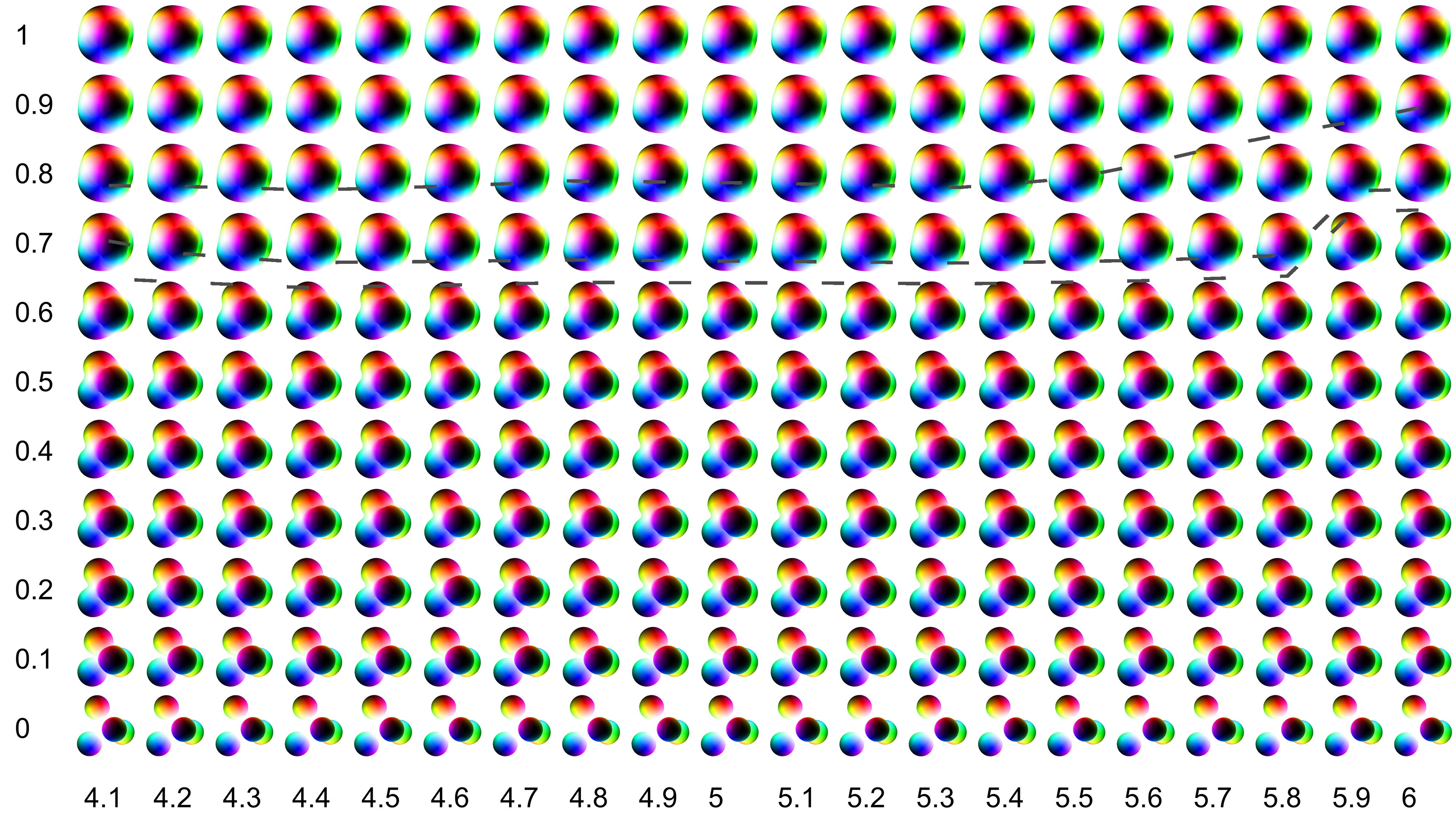
Figure 13: Baryon charge density isosurfaces of the 4-Skyrmion solutions over part of the scanned parameter space. The vertical axis denotes the values of $c_{6}$ while the horizontal axis is $m_{2}$. The dashed lines show contours of $\sigma^{O_{h}}=0.1,0.5,1$ from top to bottom. The center of mass of the Skyrmion corresponds to its position in parameter space.

The solutions obtained and presented here are made on a square grid in parameter space with $c_{6}=0,0.1,0.2,\ldots,1$ and $m_{2}=0,0.1,0.2,\ldots,6$, yielding a total of 671 numerical solutions. The baryon charge density isosurfaces are shown in figs. 11–13. As mentioned in the previous section, the initial condition for the 4-Skyrmion at the point $(m_{2},c_{6})=(0,0)$ is given by the rational map Ansatz (19)–(21).

The figures in this section are contour plots in the parameter space with $m_{2}$ being the abscissa and $c_{6}$ being the ordinate. On all figures, we will overlay three lines with the order parameter, $\sigma^{O_{h}}$, which measures if the solutions possess octahedral symmetry ($\sigma^{O_{h}}=0$) or remain only tetrahedrally symmetric ($\sigma^{O_{h}}>0$). From the top of the figures and down, the curves correspond to $\sigma^{O_{h}}=0.1,0.5,1$.

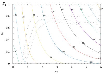
(a)

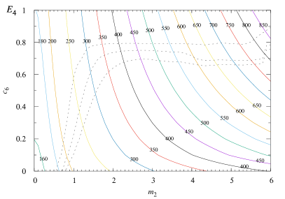
(b)

Figure 2: Energies of the (a) 1-Skyrmion and (b) 4-Skyrmion in Skyrme units. The dashed lines show contours of $\sigma^{O_{h}}=0.1,0.5,1$ from top to bottom.

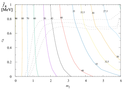
(a)

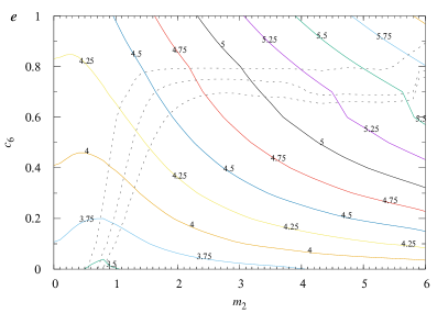
(b)

Figure 3: Calibration constants (a) $\tilde{f}_{\pi}$ [MeV] and (b) the Skyrme coupling constant $e$. The dashed lines show contours of $\sigma^{O_{h}}=0.1,0.5,1$ from top to bottom.

First we plot the classical energies (masses) of the 1-Skyrmion and the 4-Skyrmion in Skyrme units in fig. 2 just to get a feel for how the energy changes in parameter space before calibrating the model. Both figures show isocurves according to our expectation, i.e. the energy increases roughly in quadrature from the contribution due to the loosely bound potential with coefficient $m_{2}^{2}$ and from the BPS-Skyrme term with coefficient $c_{6}$. The increase in energy, nevertheless, is quite drastic. If we compare the $(m_{2},c_{6})=(0,0)$ point with the $(m_{2},c_{6})=(6,1)$ point, the energy increases with a factor of $5.42$ for the 1-Skyrmion and $5.95$ for the 4-Skyrmion.

In fig. 3 the calibration constants, i.e. the pion decay constant, $\tilde{f}_{\pi}$ and the Skyrme coupling constant $e$, are shown in the parameter space. It is interesting that for small $m_{2}<1$, the pion decay constant (see fig. 3(a)) with our calibration convention is almost independent of $c_{6}$. What happens in this regime is that the sextic term increases both the size and the energy of the 4-Skyrmion such that the ratio is almost constant $r_{4}(c_{6})/E_{4}(c_{6})\propto{\rm const}$. For large $m_{2}$, however, the mass of the 4-Skyrmion increases faster than the radius and hence the above-mentioned linear relation no longer holds; as a result the pion decay constant decreases for increasing $c_{6}$. If we now hold $c_{6}$ fixed, an increase in $m_{2}$ increases the mass and reduces the size of the Skyrmions and hence always leads to a decrease in the pion decay constant. The combined behavior is displayed in fig. 3(a). The pion decay constant is underestimated everywhere, since in the pion vacuum its experimentally measured value is about 184 MeV.

The Skyrme coupling constant $e$ is shown in fig. 3(b) and depends on the product of the size and the energy of the 4-Skyrmion and hence displays a different behavior. For small $c_{6}\ll 1$, the increase in $m_{2}$ has a mild behavior since the loosely bound potential both increases the mass and reduces the size of the Skyrmions. For $c_{6}=0$ and $m_{2}\lesssim 0.7$ the coupling reduces slightly with increasing $m_{2}$, whereas for $m_{2}>0.7$ the coupling starts to increase. This behavior for constant slices of $c_{6}$ is continued but the turning point ($0.7$ above) moves slightly downwards as $c_{6}$ is increased. For finite $c_{6}$ the increase in $m_{2}$ now leads to a larger increase in the coupling $e$.

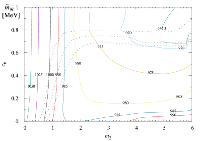
(a)

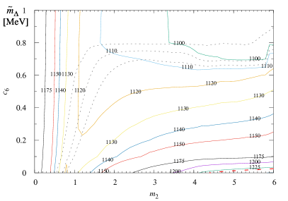
(b)

Figure 4: (a) Nucleon mass, $\tilde{m}_{N}$ [MeV] and (b) $\Delta$ mass, $\tilde{m}_{\Delta}$ [MeV]. The thick red dashed line in (b) is the experimentally measured mass of the $\Delta$ resonance ($\tilde{m}_{\Delta}^{\rm exp}\simeq 1232$ MeV). The dashed lines show contours of $\sigma^{O_{h}}=0.1,0.5,1$ from top to bottom.

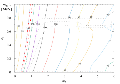
(a)

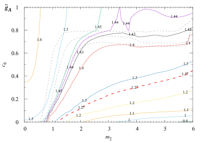
(b)

Figure 5: (a) pion mass, $\tilde{m}_{\pi}$ [MeV] and (b) axial coupling $\tilde{g}_{A}$. The thick red dashed lines in (a) are the experimentally measured pion masses ($\tilde{m}_{\pi}^{\rm exp}\simeq 135.0\;\textrm{MeV},139.6\;\textrm{MeV}$) and in (b) the experimentally measured axial coupling of the nucleon ($\tilde{g}_{A}^{\rm exp}\simeq 1.27$) PDG:2015 . The dashed lines show contours of $\sigma^{O_{h}}=0.1,0.5,1$ from top to bottom.

We will now show the spectrum of the model, starting in fig. 4 with the nucleon mass and the $\Delta$ mass. The nucleon mass (fig. 4(a)) in our calibration scheme is tightly related to the total binding energy (QRBE), because we fit the mass and size of the 4-Skyrmion to those of Helium-4. Therefore, once the binding energy is right, then so is the nucleon mass. We will thus discuss this in more detail shortly, but let us mention that in the top-right part of the parameter space, i.e. for large $m_{2}$ and large $c_{6}$, the nucleon mass is only overestimated by about 28 MeV, which is about $3\%$ above the experimentally measured value.

The $\Delta$ mass is shown in fig. 4(b). First of all, we should warn the reader about identifying this spin excitation of the 1-Skyrmion with the $\Delta$ resonance, as it may be inherently inconsistent (see also the discussion). Nevertheless, we will show the results for completeness. As usual in a Skyrme-like model with this interpretation of the $\Delta$, its mass is underestimated. What is worse is that where the binding energy and nucleon mass tend to their experimentally measured values, the $\Delta$ mass tends to be the smallest and hence farthest from its true value.

The pion mass is shown in fig. 5(a). In our chosen calibration scheme, the dependence on $c_{6}$ is mild and it mostly depends on the value of $m_{2}$; that is, the pion mass decreases for increasing $m_{2}$. For $m_{2}\simeq 0.5$–$1$, the pion mass fits well with the experimentally measured value for our choice of $m_{1}=1/4$. In order to get a more physical value of the pion mass in the top-right corner of the parameter space, we could increase the value of $m_{1}$ to say about 0.5 in order to compensate the decrease in the physical value caused by the loosely bound potential. We have not done this, as this is not a pressing issue for the model at the moment; the value of the pion decay constant is very far from its experimental value and the QRBE is not quite at the physical values either. One attitude about the low-energy constants (LECs) is that they should be “renormalized” to the in-medium conditions that the inside of the baryons possess. If this really justifies the pion decay constant to differ by more than factors of two (four) from its experiment value, then the same may apply to the pion mass.

The axial coupling of the nucleon is shown in fig. 5(b). In the region of parameter space where the sextic term dominates ($c_{6}\sim 1$ and $m_{2}=0$), the axial coupling is generally too large (however, this may change for larger values of $c_{6}$ than studied here), whereas for large $m_{2}$, $c_{6}=0$ the axial coupling is generally too small. In the top-right corner of parameter space where the binding energy turns out to be smallest, the axial coupling takes on intermediate values. Unfortunately, the experimentally measured value (thick red dashed line) is reached just after the cubic symmetry of the 4-Skyrmion is lost.

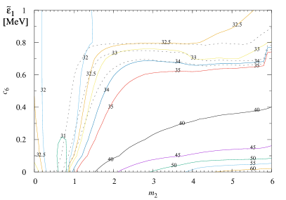
(a)

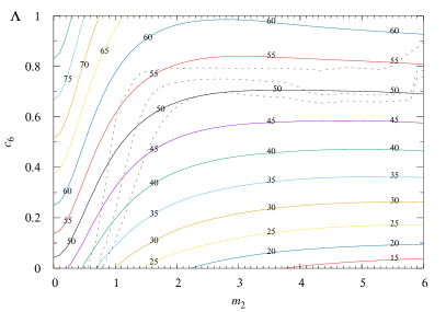
(b)

Figure 6: (a) Quantum isospin correction to the nucleon mass, $\tilde{\epsilon}_{1}$ [MeV] and (b) the diagonal of the isospin inertia tensor of the 1-Skyrmion, $\Lambda$, in Skyrme units. The dashed lines show contours of $\sigma^{O_{h}}=0.1,0.5,1$ from top to bottom.

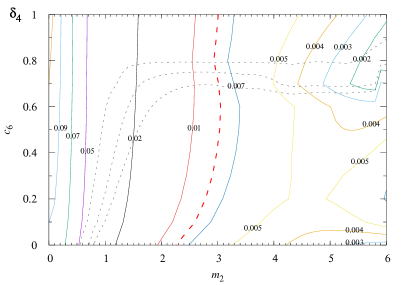
(a)

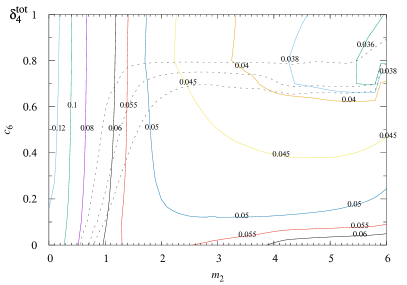
(b)

Figure 7: (a) (CRBE) Classical and (b) (QRBE) quantum relative binding energy of the 4-Skyrmion. The thick red dashed line in (a) is the experimental binding energy of Helium-4 ($\delta_{4}^{\rm exp}\simeq 0.008$) (it should not be compared to the CRBE but to the QRBE; it is shown just for reference). The dashed lines show contours of $\sigma^{O_{h}}=0.1,0.5,1$ from top to bottom.

The quantum mass correction to the nucleon as a 1-Skyrmion is shown in fig. 6(a) and the diagonal value of the isospin inertia tensor, $\Lambda$ is shown in fig. 6(b). The two quantities are related by eq. (26). As already mentioned, there are two limits where the classical binding energy can become infinitesimally small: the point particle model limit (PPML) which corresponds to $c_{6}$ fixed, $m_{2}\to\infty$; and the BPS-Skyrme model limit (BSML) which corresponds to $c_{6}/m_{2}$ fixed, $m_{2}\to\infty$. It is interesting to see – within the calibration scheme adopted here – that the direction of the BPS-Skyrme model limit reaches quantum mass corrections to the 1-Skyrmion which are almost half the values obtained in the point particle model limit. If this strategy for obtaining a physically sensible Skyrme model is correct, it is important to see where the quantum correction to the 1-Skyrmion can be suppressed enough to reach physically measured values of the binding energies. This viewpoint is typical for a purist particle physicist who prefers as little fine tuning as possible. Other possibilities are of course that the physics at the atomic scale is highly fine tuned and there are big corrections to both the 1-Skyrmions and the $B$-Skyrmions canceling each other out almost precisely, leaving behind binding energies at the 1-percent level (see also the discussion).

The quantity $\tilde{\epsilon}_{1}$ contains both the energy unit, the value of the Skyrme coupling and the isospin inertia tensor’s diagonal value. In order to disentangle the various effects, we show the value of the diagonal of the isospin inertia tensor, $\Lambda$, in fig. 6(b). As $\tilde{\epsilon}_{1}\propto\Lambda^{-1}$, we can see that, overall, the above mentioned behavior indeed stems from $\Lambda$ and not peculiarities of the calibration. That is, the smallness of the quantum correction in the BPS-Skyrme model limit comes from the fact that $\Lambda$ is bigger than in the point particle model limit. This fact, in turn, can be traced directly to the fact that the Skyrmions become larger when a sizable sextic term (BPS-Skyrme term) is included and they become smaller when a strong loosely bound potential is turned on.

We are now ready to present one of the main results of the paper, namely the relative binding energies in fig. 7. In this part of parameter space, the CRBE (fig. 7(a)) is almost independent of $c_{6}$. That is, only cranking up the sextic term does not reduce the CRBE but in fact – in this calibration scheme – it leads to a slight increase in the binding energy. The effect is quite mild though. The explanation is that the sextic term just makes the Skyrmions larger and heavier; however, after the calibration this effect is almost swallowed up. The loosely bound potential, on the other hand, does its job very well. The CRBE is reduced to the 1-percent level around $m_{2}\sim 2$–$2.6$ depending on the value of $c_{6}$, and it reaches values slightly below $0.2\%$ for $m_{2}\sim 6$. Now the sextic term is crucial for what happens. If we solely include the loosely bound potential, the model loses the platonic symmetries of the Skyrmions and the Skyrmions become well separated point particles. However, if we turn on the BPS-Skyrme term, the 4-Skyrmion can retain its cubic symmetry and possess a CRBE below the 1-percent level. The upper black dashed line shows the symmetry order parameter for $\sigma^{O_{h}}=0.1$ and the cubic symmetry can also be observed in figs. 11–13.

The problem of the binding energies is not quite solved yet, because we have to identify the quantum state of the Skyrmion with the nuclear particle. This, in particular, means that all binding energies are relatively increased by the fact that the nucleon receives a quantum correction for being a spin-$\tfrac{1}{2}$ particle in the ground state. This means that if it is a consistent treatment not to include any other quantum corrections (which is probably not the case), then we must find a point in the parameter space where the quantum mass correction to the 1-Skyrmion is at the 1-percent level. In fig. 7(b) we can see that the discussion of the quantum correction $\tilde{\epsilon}_{1}$ carries directly over to the QRBE. In particular, in the direction of the point particle model limit ($c_{6}=0$, $m_{2}\to\infty$) the QRBE we reach in the parameter space is only as low as slightly below $6\%$, whereas in the direction of the BPS-Skyrme model limit ($c_{6}\propto m_{2}\to\infty$) the QRBE reaches values as low as $3.6\%$, which for Helium-4 should be compared to about $0.8\%$ (experimental value), i.e. about $2.8\%$ over-binding. This is, however, the level of over-binding also sometimes present in nuclear models like the ab initio no-core shell model, see e.g. Ref. Barrett:2013nh .

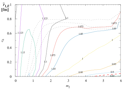
(a)

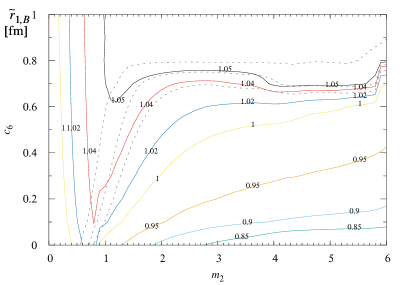
(b)

Figure 8: (a) ($\tilde{r}_{1,E}$) Electric and (b) ($\tilde{r}_{1,B}$) baryon charge radii of the proton. The thick red dashed line in (a) is the experimentally measured charge radius of the proton (CODATA) ($\tilde{r}_{1,E}^{\rm exp}\simeq 0.875$ fm) PDG:2015 . The dashed lines show contours of $\sigma^{O_{h}}=0.1,0.5,1$ from top to bottom.

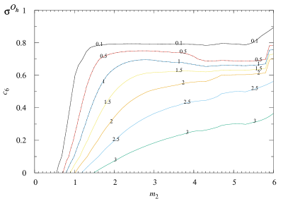
(a)

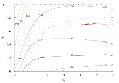
(b)

Figure 9: (a) Order parameter for octahedral symmetry, $\sigma^{O_{h}}$, and (b) diagonal component $v$ of the spin inertia tensor of the 4-Skyrmion, $V_{ij}=v\delta^{ij}$, in Skyrme units. The dashed lines show contours of $\sigma^{O_{h}}=0.1,0.5,1$ from top to bottom.

We will now turn to the electric charge radius of the proton, which is shown in fig. 8(a). In the Skyrme model it has half its contribution from the baryon charge density and the other half from the vector charge corresponding to the isospin, see eq. (29). It is interesting to see that we can obtain the best QRBE for large $m_{2}$ and large $c_{6}$ and hence also the best nucleon mass, but the physically measured value of the electric charge radius of the proton is reached spot-on in the direction of the point particle model limit; that is for $c_{6}=0$ and $m_{2}\sim 5$–$6$. In all other parts of parameter space, the 1-Skyrmion size is generally overestimated. This is due to the fact that $B$-Skyrmions tend to be too small and the 4-Skyrmion is no exception. Due to the calibration where we fit the size of the 4-Skyrmion to that of Helium-4, the 1-Skyrmion is thus generally too large. It is interesting, nevertheless, to see that the point particle model limit gets the proton size right.

The baryon charge radius is not physically measurable, but it is a component of the electric charge radius of the proton. For large $m_{2}$, we can see that their behaviors are comparable, see fig. 8(b).

The last but important observable we will study here is our proposal for an order parameter for the symmetry breaking of the cubic (octahedral) symmetry of the 4-Skyrmion, see eq. (39). By comparing the symmetries observed in the figures 11–13 with the values seen in fig. 9(a), we see that for $\sigma^{O_{h}}<0.1$ the 4-Skyrmion possesses cubic symmetry, which is the upper black dashed line shown on all figures. Let us mention that in the region of parameter space to the top-left of the upper black dashed line, $\sigma^{O_{h}}$ is very close to zero everywhere, except close to the dashed line and the deviation here is merely numerical error. For $\sigma^{O_{h}}\gtrsim 0.5$ the loss of octahedral symmetry is visible to the naked eye, see figs. 11–13.

For completeness we display the values of the inertia tensors in the parameter space in figs. 9(b) and 10. Throughout the scanned part of the parameter space, we have that $V_{ij}=v\delta^{ij}$ is diagonal and $W_{ij}=0$ vanishes, whereas the two nonzero values of the isospin tensor of inertia are $U_{11}=U_{22}$ and $U_{33}$. We can see from fig. 10 that $U_{11}$ is in general different from $U_{33}$ except in the region of parameter space where $c_{6}$ is small and $m_{2}$ is large.

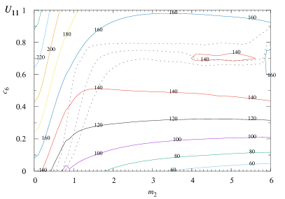
(a)

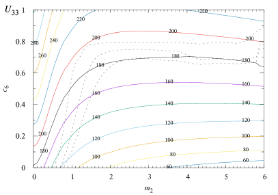
(b)

Figure 10: (a) $U_{11}=U_{22}$ and (b) $U_{33}$ of the isospin inertia tensor of the 4-Skyrmion in Skyrme units. The dashed lines show contours of $\sigma^{O_{h}}=0.1,0.5,1$ from top to bottom.

4 Discussion

In this paper, we have made an extensive parameter scan of the generalized Skyrme model with the loosely bound potential by performing full PDE calculations. The full numerical calculations are necessary for detecting the symmetries of the Skyrmions, in particular, whether the 4-Skyrmion possesses the sought-for cubic symmetry or it loses it becoming a tetrahedrally symmetric object of “point” particles. In ref. Gudnason:2016tiz we made an initial study of the parameter space limited to $m_{2}\leq 1$ using the rational map Ansatz for the cube, under the assumption that the symmetries would stay unchanged in such a limited part of parameter space. That assumption turned out to be true indeed. In this paper, we have been able to go much further into the direction of turning up the loosely bound potential and hence reducing the binding energies significantly. As expected from ref. Gudnason:2016mms , the loosely bound potential itself will quickly break the cubic symmetry of the 4-Skyrmion. Fortunately, it turns out that turning on a finite sextic term makes the 4-Skyrmion resistant to the impending symmetry breaking a long way up in $m_{2}$, the (square-root of the) coefficient of the loosely bound potential.

The philosophy that we have used as a guiding principle is to keep as much symmetry as possible whilst reducing the binding energies as much as possible; we try to cling on to the platonic symmetries possessed by the Skyrmions of small $B$ ($B<8$) and in particular the cubic symmetry of the 4-Skyrmion. Next we note that the classical relative binding energy (CRBE) is almost independent of the sextic term with coefficient $c_{6}$, but depends strongly on the loosely bound potential with coefficient $m_{2}^{2}$. Now as a direct test for whether the above stated philosophy is justified experimentally, we can compare two limits: the point particle model limit (PPML) ($c_{6}=0$ and $m_{2}\to\infty$) and the BPS-Skyrme model limit (BSML) ($c_{6}\propto m_{2}\to\infty$). Of course we have not taken any strict limit and just considered $m_{2}$ large ($m_{2}\simeq 6$) and the BSML case here will refer to $c_{6}=1$, $m_{2}=6$. First of all, we find that although the CRBE is almost the same in the two cases, the QRBE receives a larger quantum contribution in the PPML case than in the BSML case. This fact is intimately related to the value of the isospin inertia tensor being larger when the sextic term is turned on, which in turn is due to the sextic term enlarging the Skyrmions. The nucleon mass correlates with the binding energy in our calibration scheme and hence is closer to the measured value in the BSML case (but still overestimated) than in the PPML case. On the other hand, the pion decay constant is larger (but still underestimated) in the PPML case than in the BSML case and the electric charge radius is almost spot-on the experimental value in the PPML corner of our parameter space. Finally there is a tie between the two cases for the axial coupling of the nucleon, for which it is overestimated in the BSML case and underestimated in the PPML case. We present in table 1 four benchmark points compared to experimental data, including the PPML and BSML cases.

Table 1: Benchmark points compared to experimental data. The model points are: A [SSM] Standard Skyrme Model; B [GSM] Generalized Skyrme Model; C [PPML] Point Particle Model Limit; D [BSML] BPS-Skyrme Model Limit.

	Point A [SSM]		Point B [GSM]		Point C [PPML]		Point D [BSML]
	$(m_{2},c_{6})=(0,0)$		$(m_{2},c_{6})=(0,1)$		$(m_{2},c_{6})=(6,0)$		$(m_{2},c_{6})=(6,1)$
$\tilde{f}_{\pi}$	$-32$.	$1\%$	$-51$.	$0\%$	$-80$.	$8\%$	$-86$.	$5\%$
$\tilde{m}_{N}$	$+12$.	$0\%$	$+13$.	$9\%$	$+6$.	$2\%$	$+2$.	$9\%$
$\tilde{m}_{\Delta}$	$-3$.	$8\%$	$-2$.	$6\%$	$+1$.	$6\%$	$-11$.	$0\%$
$\tilde{m}_{\pi}^{\pm}$	$+14$.	$7\%$	$+39$.	$9\%$	$-51$.	$7\%$	$-46$.	$2\%$
$\tilde{m}_{\pi}^{0}$	$+18$.	$6\%$	$+44$.	$7\%$	$-50$.	$1\%$	$-44$.	$4\%$
$\tilde{g}_{A}$	$+17$.	$4\%$	$+30$.	$3\%$	$-30$.	$0\%$	$+13$.	$6\%$
$\delta_{4}$	$+970$.	$3\%$	$+1174$.	$5\%$	$-67$.	$7\%$	$-72$.	$5\%$
$\delta_{4}^{\rm tot}$	$+1331$.	$4\%$	$+1514$.	$6\%$	$+725$.	$7\%$	$+348$.	$9\%$
$\tilde{r}_{1,E}$	$+27$.	$8\%$	$+25$.	$3\%$	$-4$.	$2\%$	$+23$.	$0\%$

For the observables considered in this paper, it is not clear that preserving as much symmetry as possible is better in line with phenomenology. Both the cases summarized above have their merits. Nevertheless, once the full quantum excitational spectrum is considered for the nuclei, it becomes clear that having a large symmetry is not just aesthetics but a necessity. This was pointed out recently in ref. Gudnason:2018aej ; in this particular case, the lack of a symmetry of rank four resulted in parity doubling of the states – not observed in Nature.

A completely different way to try to solve the binding energy problem of the Skyrmions is to disregard the classical energies completely and believe that the true quantum states have very large corrections to their classical counterparts. This solution may well be the true description of nuclear physics although it runs against conventional particle physics wisdom that prefers natural mechanisms as explanations for physical effects. A known counterexample for naturalness indeed in nuclear physics is the fact that the binding energy of the triplet deuteron is about 2.2 MeV whereas the energy released in neutron beta decays is about 1.3 MeV. That 0.9 MeV difference is what kept all the neutrons from decaying during the evolution of the Universe and be missing in the formation of countless elements. Of course our Universe may just well be a giant accident. As we discussed in the introduction, the question of whether semi-classical quantization with the perturbative addition of a few light modes of the soliton is a good approximation comes down to whether the fluctuation spectrum is “weakly coupled”. It would be an important next step to investigate this issue in depth.

The $\Delta$ resonance is at best problematic in the Skyrme model. The reason for this is evident from our discussion about trying to reduce the quantum isospin contribution to the mass of the nucleon and is rooted in eq. (28). That is, if we make $\tilde{\epsilon}_{1}$ small then so is $5\tilde{\epsilon}_{1}$, see ref. Adam:2016drk ; more concretely, if we want the spin/isospin contribution to the mass of the nucleon, $\tilde{\epsilon}_{1}$, to be less than the binding energy of roughly 16 MeV, which is approximately the binding energy of nuclear matter, then it is impossible for $5\tilde{\epsilon}_{1}$ to be as large as 366 MeV Adam:2016drk . As further pointed out in ref. Adam:2016drk , the $\Delta$ resonance probably needs a fully relativistic treatment and should be considered as a resonance with a complex mass pole.

Considering larger coefficients of the sextic BPS-Skyrme term is a natural continuation of this work and it may show qualitatively interesting new behavior of the model. If the BPS-Skyrme term and the potential term become too large, however, one enters the near-BPS regime of the BPS-Skyrme model which is known to be technically difficult. In the light of the discussions in this paper, the more important question is whether it is necessary to obtain solutions with very low classical binding energies – like in this paper – or the true solution to the quantum physics of nuclei lies in sizable corrections that perhaps via beautiful symmetries somehow all balance in such a way as to give small binding energies at the 1-percent level for all nuclei. This will be left as work for the future.

We should remind the reader that we did not get the physical pion mass right in the region of parameter space with small binding energies. This can easily be fixed, but the change for the rest of the physics is expected to be insignificant and as long as the pion decay constant is so far from its measured value, it remains a question whether the pion mass should be close to its experimental value or not. Lattice-QCD simulations often get good results even though their pion mass is typically much too large compared with the experimental value.

There are lots of directions to consider for improving the Skyrme model in order for it to become a full-fledged high-precision model of nuclear physics. If the program succeeds, it will become a few-parameter model which basically can cover all nuclei. The list of problems is however not so short. The problem of the binding energy that we have worked on in this paper is not solved yet and we are probably getting closer to a point where we can determine whether the Skyrme model is natural and hence the quantum corrections somehow are small as expected in systems with semi-classical quantization, or there are relatively large quantum corrections that just happen to balance out almost perfectly over a large variety of nuclei – many possessing different symmetries.

The small isospin breaking present in Nature still remains largely unincorporated in the Skyrme model. The recent suggestion by Speight Speight:2018zgc is based on including the $\omega$ meson and an explicit symmetry breaking term. This direction of improving the Skyrme model is also considered for solving the binding energy problem. That is, including vector mesons in the model, see e.g. Naya:2018mpt where $\rho$ mesons are considered.

A further improvement to be considered, which will become more important for the studies of large nuclei, is to include the effects of the Coulomb energy. Although it is known how to calculate the Coulomb force for multi-Skyrmions, it should ideally be back-reacted onto the Skyrmions. This would require some partial gauging and further complicate the model.

It would also be interesting to consider other Skyrmions than the 4-Skyrmion, in order to check our claims about the preservation of symmetries in the model. A preliminary study suggests that for the 8-Skyrmion, the two cubes retain their separate octahedral symmetries but become more weakly bound to each other with the result that, in the low-binding energy regime, the chain and twisted chain become almost degenerate in energies. There are plenty of other Skyrmions that would be interesting to study.

The question, however, remains: how to resolve the quantum part of the binding-energy problem for Skyrmions as nuclei? Hopefully, this question may be answered in the future.

Acknowledgments

S. B. G. thanks Chris Halcrow for discussions. S. B. G. is supported by the Ministry of Education, Culture, Sports, Science (MEXT)-Supported Program for the Strategic Research Foundation at Private Universities “Topological Science” (Grant No. S1511006) and by a Grant-in-Aid for Scientific Research on Innovative Areas “Topological Materials Science” (KAKENHI Grant No. 15H05855) from MEXT, Japan. The calculations in this work were carried out using the TSC computing cluster of the “Topological Science” project at Keio University.

References

- (1) T. H. R. Skyrme, “A Unified Field Theory of Mesons and Baryons,” Nucl. Phys. 31, 556 (1962).
- (2) T. H. R. Skyrme, “A Nonlinear field theory,” Proc. Roy. Soc. Lond. A 260, 127 (1961).
- (3) E. Witten, “Global Aspects of Current Algebra,” Nucl. Phys. B 223, 422 (1983).
- (4) E. Witten, “Current Algebra, Baryons, and Quark Confinement,” Nucl. Phys. B 223, 433 (1983).
- (5) E. Braaten, S. Townsend and L. Carson, “Novel Structure of Static Multi - Soliton Solutions in the Skyrme Model,” Phys. Lett. B 235, 147 (1990).
- (6) C. J. Houghton, N. S. Manton and P. M. Sutcliffe, “Rational maps, monopoles and Skyrmions,” Nucl. Phys. B 510, 507 (1998) [hep-th/9705151].
- (7) R. Battye, N. S. Manton and P. Sutcliffe, “Skyrmions and the alpha-particle model of nuclei,” Proc. Roy. Soc. Lond. A 463, 261 (2007) [hep-th/0605284].
- (8) D. T. J. Feist, P. H. C. Lau and N. S. Manton, “Skyrmions up to Baryon Number 108,” Phys. Rev. D 87, 085034 (2013) [arXiv:1210.1712 [hep-th]].
- (9) P. H. C. Lau and N. S. Manton, “States of Carbon-12 in the Skyrme Model,” Phys. Rev. Lett. 113, 232503 (2014) [arXiv:1408.6680 [nucl-th]].
- (10) C. J. Halcrow, C. King and N. S. Manton, “A dynamical -cluster model of 16O,” Phys. Rev. C 95, 031303 (2017) [arXiv:1608.05048 [nucl-th]].
- (11) J. I. Rawlinson, “An Alpha Particle Model for Carbon-12,” Nucl. Phys. A 975, 122 (2018) [arXiv:1712.05658 [nucl-th]].
- (12) P. Sutcliffe, “Skyrmions, instantons and holography,” JHEP 1008, 019 (2010) [arXiv:1003.0023 [hep-th]].
- (13) P. Sutcliffe, “Skyrmions in a truncated BPS theory,” JHEP 1104, 045 (2011) [arXiv:1101.2402 [hep-th]].
- (14) C. Naya and P. Sutcliffe, “Skyrmions in models with pions and rho mesons,” arXiv:1803.06098 [hep-th].
- (15) C. Adam, J. Sanchez-Guillen and A. Wereszczynski, “A Skyrme-type proposal for baryonic matter,” Phys. Lett. B 691, 105 (2010) [arXiv:1001.4544 [hep-th]].
- (16) C. Adam, J. Sanchez-Guillen and A. Wereszczynski, “A BPS Skyrme model and baryons at large ,” Phys. Rev. D 82, 085015 (2010) [arXiv:1007.1567 [hep-th]].
- (17) D. Harland, “Topological energy bounds for the Skyrme and Faddeev models with massive pions,” Phys. Lett. B 728, 518 (2014) [arXiv:1311.2403 [hep-th]].
- (18) M. Gillard, D. Harland and M. Speight, “Skyrmions with low binding energies,” Nucl. Phys. B 895, 272 (2015) [arXiv:1501.05455 [hep-th]].
- (19) S. B. Gudnason, “Loosening up the Skyrme model,” Phys. Rev. D 93, 065048 (2016) [arXiv:1601.05024 [hep-th]].
- (20) M. F. Atiyah and N. S. Manton, “Geometry and kinematics of two skyrmions,” Commun. Math. Phys. 153, 391 (1993).
- (21) T. Sakai and S. Sugimoto, “Low energy hadron physics in holographic QCD,” Prog. Theor. Phys. 113, 843 (2005) [hep-th/0412141].
- (22) L. Bartolini, S. Bolognesi and A. Proto, “From the Sakai-Sugimoto Model to the Generalized Skyrme Model,” Phys. Rev. D 97, 014024 (2018) [arXiv:1711.03873 [hep-th]].
- (23) C. Adam and A. Wereszczynski, “Topological energy bounds in generalized Skyrme models,” Phys. Rev. D 89, 065010 (2014) [arXiv:1311.2939 [hep-th]].
- (24) M. Gillard, D. Harland, E. Kirk, B. Maybee and M. Speight, “A point particle model of lightly bound skyrmions,” Nucl. Phys. B 917, 286 (2017) [arXiv:1612.05481 [hep-th]].
- (25) S. Baldino, S. Bolognesi, S. B. Gudnason and D. Koksal, “Solitonic approach to holographic nuclear physics,” Phys. Rev. D 96, 034008 (2017) [arXiv:1703.08695 [hep-th]].
- (26) S. B. Gudnason and M. Nitta, “Modifying the pion mass in the loosely bound Skyrme model,” Phys. Rev. D 94, 065018 (2016) [arXiv:1606.02981 [hep-ph]].
- (27) S. B. Gudnason, B. Zhang and N. Ma, “Generalized Skyrme model with the loosely bound potential,” Phys. Rev. D 94, 125004 (2016) [arXiv:1609.01591 [hep-ph]].
- (28) C. Barnes and N. Turok, “A Technique for calculating quantum corrections to solitons,” [hep-th/9711071].
- (29) C. J. Halcrow, “Vibrational quantisation of the B = 7 Skyrmion,” Nucl. Phys. B 904, 106 (2016) [arXiv:1511.00682 [hep-th]].
- (30) S. B. Gudnason and C. Halcrow, “ Skyrmion as a two-cluster system,” Phys. Rev. D 97, 125004 (2018) [arXiv:1802.04011 [hep-th]].
- (31) R. F. Dashen, B. Hasslacher and A. Neveu, “Nonperturbative Methods and Extended Hadron Models in Field Theory 2. Two-Dimensional Models and Extended Hadrons,” Phys. Rev. D 10, 4130 (1974).
- (32) S. B. Gudnason, M. Nitta and N. Sawado, “Black hole Skyrmion in a generalized Skyrme model,” JHEP 1609, 055 (2016) [arXiv:1605.07954 [hep-th]].
- (33) C. Adam, O. Kichakova, Y. Shnir and A. Wereszczynski, “Hairy black holes in the general Skyrme model,” Phys. Rev. D 94, 024060 (2016) [arXiv:1605.07625 [hep-th]].
- (34) G. H. Derrick, “Comments on nonlinear wave equations as models for elementary particles,” J. Math. Phys. 5, 1252 (1964).
- (35) A. Vilenkin and E. P. S. Shellard, “Cosmic Strings and Other Topological Defects,” Cambridge Monographs (2000).
- (36) G. S. Adkins, C. R. Nappi and E. Witten, “Static Properties of Nucleons in the Skyrme Model,” Nucl. Phys. B 228, 552 (1983).
- (37) B. R. Barrett, P. Navratil and J. P. Vary, “Ab initio no core shell model,” Prog. Part. Nucl. Phys. 69, 131 (2013).
- (38) K. A. Olive et. al. (Particle Data Group), Chin. Phys. C, 38, 090001 (2014).
- (39) C. Adam, J. Sanchez-Guillen and A. Wereszczynski, “On the spin excitation energy of the nucleon in the Skyrme model,” Int. J. Mod. Phys. E 25, 1650097 (2016) [arXiv:1608.00979 [nucl-th]].
- (40) J. M. Speight, “A simple mass-splitting mechanism in the Skyrme model,” Phys. Lett. B 781, 455 (2018) [arXiv:1803.11216 [hep-th]].