Model averaging for robust extrapolation in evidence synthesis

Abstract

[Summary] Extrapolation from a source to a target, e.g., from adults to children, is a promising approach to utilizing external information when data are sparse. In the context of meta-analysis, one is commonly faced with a small number of studies, while potentially relevant additional information may also be available. Here we describe a simple extrapolation strategy using heavy-tailed mixture priors for effect estimation in meta-analysis, which effectively results in a model-averaging technique. The described method is robust in the sense that a potential prior-data conflict, i.e., a discrepancy between source and target data, is explicitly anticipated. The aim of this paper is to develop a solution for this particular application, to showcase the ease of implementation by providing R code, and to demonstrate the robustness of the general approach in simulations.

, , and (2017), Model averaging for robust extrapolation in evidence synthesis, Statistics in Medicine, 2018;00:0–0.

1 Introduction

When empirical evidence is sparse, it may be useful to be able to utilize related source data to extrapolate to the targeted population. This is especially relevant in the context of rare diseases or small populations, but the problem is common in many applications. Several regulatory guidelines touch upon the problem from different angles, either explicitly concerning extrapolation ¹ and the use of external data ², or, for example, in the contexts of small populations research ³, paediatric studies ⁴, or bridging studies ⁵. The potential benefits of extrapolation approaches are generally recognized ^{6, 7}, especially in the context of rare diseases ^{8, 9}. Concerning the methodological aspect, the use of Bayesian methods has frequently been suggested ^{3, 10, 11, 4, 12} and also in practice appears to be the predominant approach ¹³.

In a Bayesian model, external evidence may be considered e.g. via the formulation of informative priors or the use of hierarchical models ^{4, 13, 14, 15}. As the term extrapolation suggests, there is usually some doubt whether or to what extent the external data can or should be taken at face value and are directly applicable to the given context. Consequently, the implementation of (potential) downweighting of the external evidence is a common requirement ^{13, 16}.

So far, the literature very much focussed on the setting of a single target study, but extrapolation may also be useful in evidence synthesis. Meta-analyses are commonly based on only few studies, especially when they are concerned with rare diseases ^{17, 18}, but also quite generally ^{19, 20, 21}. Additional external data may here easily be utilized by the formulation of an informative prior distribution ^{10, 12, 11}. In the following we introduce the implementation of some degree of scepticism and robustness by using a heavy-tailed mixture prior ^{22, 23, 24}. Computationally, a mixture prior then results in a model-averaging technique ²⁵. Besides the interpretation of a “robustified” informative prior distribution, this setup may also be thought of as a combination of several data models, corresponding to subgroupings of the data into studies with common or unrelated effects ²⁶.

Encouraged e.g. by the International Rare Diseases Research Consortium (IRDiRC) ⁷, the aim of this paper is to showcase the potential of robust extrapolation in Bayesian meta-analysis via prior specification as suggested by Schmidli et al.²⁴, and to exemplify the relative ease of implementation and computation. The general idea is actually more widely applicable, beyond the context of meta-analysis. We first decribe the general methodology in Sec. 2, and then apply the approach in two case studies of meta-analyses extrapolating from external source data (adolescents or adults) to children in applications in asthma and liver transplantation in Sec. 3 and 4. In Sec. 5, the method’s long-run behaviour is investigated in a small simulation study. Sec. 6 closes with some concluding remarks. Computations are performed using R and the bayesmeta and rjags packages ^{27, 28, 29}. Example R code is available in the Appendix.

2 Bayesian random-effects meta-analysis

2.1 The model

Meta-analyses are commonly performed using the normal-normal hierarchical model (NNHM); the model may be specified as follows. A number $k$ of studies or measurements $Y_{i}$ ($i=1,\ldots,k$) are given; these measurements only come with limited accuracy, as expressed by the associated standard errors $s_{i}$. We assume that a measurement comes about as a draw from a normal distribution centered around the (study-specific) mean $\theta_{i}$:

$$Y_{i}\,|\,\theta_{i}\;\sim\;\mathrm{N}(\theta_{i},\,s_{i}^{2})\mbox{.}$$ (1)

The standard errors are commonly assumed known. The study-specific means are not necessarily identical across studies, rather one allows for a certain amount of heterogeneity between studies, implemented in terms of an additional variance component $\tau\geq 0$:

$$\theta_{i}\,|\,\mu,\,\tau\;\sim\;\mathrm{N}(\mu,\,\tau^{2})$$ (2)

^{30, 31, 32, 33}. Since often primary interest lies in the overall effect $\mu$ (and not in the shrinkage estimates of $\theta_{i}$), the model may be simplified to the marginal form

$$Y_{i}\,|\,\mu,\,\tau\;\sim\;\mathrm{N}(\mu,\,s_{i}^{2}+\tau^{2})\mbox{.}$$ (3)

There are two unknowns that one may want to infer from the data; the heterogeneity $\tau$, which commonly constitutes a nuisance parameter, and the effect $\mu$, which is usually of primary interest. In order to infer the parameters within a Bayesian framework, one needs to specify prior distributions for $\mu$ and $\tau$.

2.2 Informative priors and robustness

In the random-effects meta-analysis model we may facilitate extrapolation by propagating information through the analysis via the prior probability distribution ^{10, 12, 13}. We may have information from external sources available that can be used to inform the analysis. However, it is often uncertain whether this information is directly applicable to the present context or whether the possibility of an alternative model should also be considered ^{16, 24}. Both the utilization of additional information as well as the explicit consideration of uncertainty may also be particularly desirable in regulatory decision-making ², ³⁴.

A simple way to implement a certain amount of scepticism is via two prior components, which are combined to form the prior distribution as a mixture ^{13, 16, 35}. To that end we may formulate two parameter models, $M_{a}$ and $M_{b}$, representing the cases of equal effects for source and target data (where direct extrapolation would be valid), and of a different, unrelated effect for the new data. The two models simply differ by their assumed prior for the parameters, $p(\mu,\tau|M_{a})$ and $p(\mu,\tau|M_{b})$, respectively; the associated data model and likelihood ($p(y|\mu,\tau)$) are identical under both models. Both parameter models have prior probabilities $p(M_{a})\in[0,1]$ and $p(M_{b})=1-p(M_{a})$ associated. The marginal prior density then results as

$$p(\mu,\tau)\;=\;p(\mu,\tau|M_{a})\;p(M_{a})+p(\mu,\tau|M_{b})\;p(M_{b})$$ (4)

where the two components now are chosen such that $p(\mu,\tau|M_{a})$ is informative (with probability concentrated according to the external information), while $p(\mu,\tau|M_{b})$ is vague. The probability $p(M_{a})$ then reflects the certainty (or scepticism) associated with the external information. The same approach is readily generalized to more than two components; in the following, we will be concerned with the case of four parameter models ($M_{1},\ldots,M_{4}$) that are associated with prior probabilities $p(M_{1}),\ldots,p(M_{4})$ with $\sum_{i}p(M_{i})=1$.

A setup like this results in a heavy-tailed prior compared to $p(\mu,\tau|M_{a})$ alone; such priors have favourable properties when the data in fact do turn out to be in conflict with the prior information as supplied by $p(\mu,\tau|M_{a})$ and so it will provide more robust inference in case of a prior/data conflict ^{23, 24}.

2.3 Mixture priors and inference

A simple mixture setup has the advantage that it simplifies computations; the (conditional) posteriors under the two models $M_{a}$ and $M_{b}$ may be computed separately, and the partial results then may be re-combined via their associated Bayes factors ^{36, 24}. With that, the mixture prior effectively results in a model-averaging approach. The simplicity may be seen from the derivation via Bayes’ theorem. Consider the generic case of inferring parameters $\vartheta$ from data $y$, where the prior $p(\vartheta)$ is given as a two-component mixture distribution analogous to (4); the parameters’ posterior distribution is given by

$$p(\vartheta|y) = p(\vartheta|y,M_{a})\;p(M_{a}|y)+p(\vartheta|y,M_{b})\;p(M_{b}|y)$$ (5)

(the detailed derivation is shown in the appendix). So, from (5) one can see that with the prior set up as a two-component mixture, the posterior $p(\vartheta|y)$ again is a mixture of the two (conditional) posteriors ($p(\vartheta|y,M_{a})$ and $p(\vartheta|y,M_{b})$). The weighting results from the posterior probabilities for the two model components ($p(M_{a}|y)$ and $p(M_{b}|y)$) which again depend on the marginal likelihoods ($p(y|M_{a})$ and $p(y|M_{b})$) and the prior probabilities $p(M_{i})$:

$$p(M_{a}|y)\;=\;\frac{p(y|M_{a})\,p(M_{a})}{p(y|M_{a})\,p(M_{a})+p(y|M_{b})\,p(M_{b})}$$ (6)

where the marginal likelihoods are given by

$$p(y|M_{i})\;=\;\int p(y|\vartheta,M_{i})\,p(\vartheta|M_{i})\,\mathrm{d}\vartheta$$ (7)

(where $i\in\{a,b\}$). The approach is analogously generalized to the case of more than two mixture components.

The posterior distribution may be expressed as a mixture or weighted average of posterior components, placing the model in the class of model averaging approaches ^{25, 36, 37, 38}. The setup may be thought of as a combination of several plausible data models $M_{i}$. In this particular case, the models under consideration correspond to subgroups of the data into studies with common or unrelated parameters ²⁶. In contrast to model selection, instead of singling out a particular model for inference, model averaging then allows to perform unconditional inference by marginalizing over the uncertain model indicator.

The model averaging setup considers a discrete set of potential data models. The problem could alternatively be approached in different ways, for example, by adding further hierarchical stages to the model, which may then allow to encompass the same set of models as special cases. Conceptually, this would replace the “binary” alternatives (of exchangeable or unrelated data) by a more “continuous” notion of data similarity.

It is important to note that, due to the dependence on marginal likelihoods above, the exact specification of the “vague” prior component is crucial. The problem is related to Lindley’s paradox ³⁹: Although different vague priors may differ little in the posterior distributions they imply for the parameter vector $\vartheta$, they may still have a substantial effect on the corresponding marginal likelihoods ($p(y|M_{i})$), and with that, the eventual relative weighting of the two conditional posteriors via $p(\vartheta|y,M_{i})$. The effect may lead to somewhat counterintuitive behaviour here. While a larger prior variance for the vague model component may at first seem more conservative, it may in fact amplify the informative component’s posterior probability by reducing the marginal likelihood under the vague component.

2.4 Meta-analysis using mixture priors

2.4.1 Meta-analysis of log-ORs

In the following we will conduct meta-analyses using the random-effects model described in Sec. 2.1 with a mixture prior as described in Sec. 2.2 and 2.3. The endpoint of interest in the following is a logarithmic odds ratio (log-OR). Odds ratios and their standard errors on the logarithmic scale are computed using standard formulas ^{31, 32}. The mixture prior then is defined using components that imply different amounts or pathways of borrowing of information.

The target data set of primary interest consists of $k_{\mathrm{T}}$ effect estimates $Y_{t,1},\ldots,Y_{t,k_{\mathrm{T}}}$ and standard errors $s_{t,1},\ldots,s_{t,k_{\mathrm{T}}}$. Another set of $k_{\mathrm{S}}$ additional source estimates and standard errors ($Y_{s,i}$, $s_{s,i}$) is available, which constitutes the potentially relevant external information.

2.4.2 Prior information and data pooling

Schmidli et al.²⁴ pointed out that in the meta-analysis context consideration of external information may be implemented in two obvious ways. Firstly, in the meta-analytic-combined (MAC) approach, both source and target data sets are analyzed jointly. Alternatively, one may perform an analysis of the source data to derive an informative meta-analytic-predictive (MAP) prior distribution for the target data.

Both MAC and MAP approaches can be shown to be equivalent, since performing separate analyses and using one result to form the prior for the other (MAP approach) yields identical results to a pooled analysis (MAC approach)²⁴. This has the advantage of making the flow of information through the analysis transparent, and it also may be utilized to simplify computations. Use of an informative prior (based on source data) may then technically also be viewed as a “pooling” of source and target data.

2.4.3 Vague prior

The vague prior ($p(\mu,\tau|M_{4})$ in the following) is specified as uninformative, covering a range of a priori plausible values. In the following, we represent an uninformative prior by a zero-mean normal distribution with standard deviation 2 for the effect $\mu$, and a half-normal distribution with scale 0.5 for the heterogeneity $\tau$. For the effect this implies a probability distribution symmetric around zero (corresponding to an odds ratio of 1) with a 95% prior probability for the log-odds ratio $\mu$ to lie within $\pm 3.92$, which translates to odds ratios roughly within a range from $\frac{1}{50}$ to $50$. This prior may be interpreted as equivalent to the information given by a contingency table of an effective sample size of 4 patients ⁴⁰. For the heterogeneity, the half-normal prior also constitutes a conservative choice in the context of log-OR endpoints ^{33, 17, 18}.

2.4.4 Mixture prior components

The informative prior components ($p(\mu,\tau|M_{i})$, $i\!<\!4$) are specified based on the posterior of a previous, separate meta-analysis, reflecting the corresponding information. This previous meta-analysis is again conducted using the vague prior $p(\mu,\tau|M_{4})$.

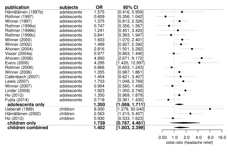
Figure 1: Forest plot for the migraine example data introduced in Sec. 3. The last three studies (Ueberall (1999), Hämäläinen (2002) and Ho (2012)) are the paediatric ones of primary interest, while the top 20 studies are the adolescents’ studies constituting the external information that may potentially be extrapolated. The endpoint of interest here is the odds ratio of headache relief for triptans vs. placebo. The combined estimate here is based on the 2-component model with $p(M_{1})=0.5$ (see also row VII in Fig. 4).

Considering the relationship between source and target data sets, a range of scenarios is conceivable; here we concentrate on a few simple possibilities. Firstly, the two data sets may be completely unrelated, so that we have two pairs of parameters ($\mu_{\mathrm{S}}$/$\tau_{\mathrm{S}}$ and $\mu_{\mathrm{T}}$/$\tau_{\mathrm{T}}$), and by analyzing one data set we cannot learn anything about the other set’s parameters. On the other hand, effect and heterogeneity may be identical in both populations ($\mu_{\mathrm{T}}=\mu_{\mathrm{S}}$ and $\tau_{\mathrm{T}}=\tau_{\mathrm{S}}$), so that we can pool the data (MAC approach), or equivalently, use the posterior from one analysis as the prior for the other (MAP approach). It may also be possible that only the effect or only the heterogeneity parameter are shared between the two populations. For the analysis of target data, this results in four possible models:

• $M_{1}$: $\mu_{\mathrm{T}}=\mu_{\mathrm{S}}$, $\tau_{\mathrm{T}}=\tau_{\mathrm{S}}$
  (informative prior for $\mu_{\mathrm{T}}$ and $\tau_{\mathrm{T}}$; “complete pooling”)

• $M_{2}$: $\mu_{\mathrm{T}}=\mu_{\mathrm{S}}$, $\tau_{\mathrm{T}}\neq\tau_{\mathrm{S}}$
  (informative prior for $\mu_{\mathrm{T}}$ only; “effect pooling”)

• $M_{3}$: $\mu_{\mathrm{T}}\neq\mu_{\mathrm{S}}$, $\tau_{\mathrm{T}}=\tau_{\mathrm{S}}$
  (informative prior for $\tau_{\mathrm{T}}$ only; “heterogeneity pooling”)

• $M_{4}$: $\mu_{\mathrm{T}}\neq\mu_{\mathrm{S}}$, $\tau_{\mathrm{T}}\neq\tau_{\mathrm{S}}$
  (vague prior; “standalone analyses”)

These four (conditional) parameter models are associated with prior probabilities $p(M_{i})$.

The eventual model setup then includes the specification of the vague prior component ($p(\mu,\tau|M_{4})$), and of the prior probabilities for the four model components $M_{i}$. Some of the model probabilities $p(M_{i})$ may be set to zero, especially for components 2 or 3.

While the parameter models $M_{1}$ and $M_{4}$ may be very obvious, reflecting the commonly faced choice between data pooling and separate analyses, the other two models deserve some more consideration. Model $M_{3}$ supports the analysis of target data by only informing the heterogeneity prior based on the source data, an approach that is familiar from previous proposals ^{41, 42}. Model $M_{2}$ is technically similar, but the scenario may be harder to motivate: a case in which the main effect is identical, but the heterogeneity is different may not be very realistic. Also, the relative similarity of models $M_{1}$ and $M_{2}$ as well as $M_{3}$ and $M_{4}$ especially in the context of relatively few observations (small $k_{\mathrm{S}}$ and $k_{\mathrm{T}}$) may be an argument in favour of a sparser model not necessarily considering all four components.

2.5 Computation

Inference within the NNHM may technically be approached in different ways, for example using stochastic integration via MCMC methods. In the following we will utilize the rjags²⁹ and bayesmeta R packages ^{28, 40}. Use of the bayesmeta package simplifies computations, but it is only applicable for a subset of models (namely those with $p(M_{2})\!=\!0$).

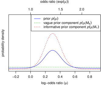
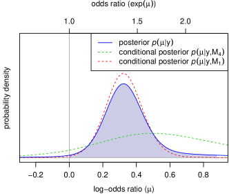
Figure 2: Prior (left) and posterior (right) densities for the example from Sec. 3. The left panel shows the prior along with its two (informative and vague) mixture components. The right panel shows the posterior, which again is a mixture of two (conditional) posteriors. The shaded area indicates the posterior 95% CI.

3 Paediatric migraine case study

3.1 Background

The data considered in the following are due to the systematic review by Richer et al.⁴³, reporting on the evidence on the effect of pharmacological medications for the treatment of acute migraine attacks in children and adolescents. Among the analyses performed is a comparison of the effect of triptans (vs. placebo) on the proportion of patients reporting headache relief. While 20 studies were found quoting odds ratios for the effect in adolescents ($12$–$17$ years of age), only 3 studies reported on headache relief in children ($<\!12$ years of age). The relevant data (numbers of cases and events, and the derived ORs) are reproduced in Tab. 3 in the appendix, the effect sizes are also illustrated in Fig. 1.

Now suppose we are interested in estimating the effect in children. Three studies constitute only a small data basis on which to judge efficacy ¹⁷, and indeed, a meta-analysis of the three studies fails to yield a conclusive result; while the odds ratio is estimated at $1.739$ (a beneficial effect), the credible interval ([$0.787$, $4.461$]) is very wide and still includes a neutral effect of $1.0$. It would be desirable if the additional adolescent studies could possibly be used to clarify whether a clinically relevant effect is present or not. In order to summarize the evidence from the adolescent studies, we can perform a meta-analysis using the vague prior from Sec. 2.4.3, which yields an estimate and 95% CI for the OR in adolescents of 1.350 [1.069, 1.711].

3.2 Analysis setup

In the present example there is a small number of target studies that are of primary interest (3 paediatric studies), and in addition there is another set of potentially relevant additional source studies available (20 studies performed in adolescent patients). The additional data provide external information, but it is not evident a priori to what extent these are directly comparable and whether extrapolation is valid. It may be plausible that the distinction between age groups is somewhat arbitrary, and that the effect ($\mu$) is indeed the same (or at least very similar) in both age groups. This uncertainty is reflected in the analysis model setup via the specification of prior probabilities $p(M_{i})$ for the different model components.

The data are in the following analyzed using a mixture of two components, considering the cases of “complete pooling” ($M_{1}$), and of two “standalone” analyses ($M_{4}$). A priori, we assume a probability of $p(M_{1})=0.5$ for the joint model, and $p(M_{4})=0.5$ for unrelated effects in adolescents and adults. With a substantial amount of scepticism associated with the prior information, we consider this a conservative choice ⁴⁴. We will also consider alternative prior setups later on.

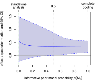
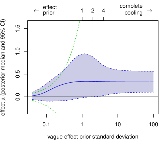
Figure 3: Diagnostic plots showing the effect of varying the prior probability $p(M_{1})$ (left panel) and the vague prior standard deviation $\sqrt{\operatorname{Var}(\mu|M_{4})}$ (right panel) in the migraine example from Sec. 3. The solid blue line shows the resulting effect estimate (log-OR), the shaded area indicates the corresponding 95% CI. The dashed green lines indicate a prior 95% range.

The two components as well as the resulting mixture prior for the effect ($\mu$) are also shown in Fig. 2 (left panel). The vague component (according to Sec. 2.4.3) is normal with zero mean and standard deviation of 2. The informative component results as the posterior from the analysis of the adolescents’ data (see Sec. 3.1).

3.3 Analysis results

Analysis of the children’s data under the two prior components yields a Bayes factor of 5.1 in favour of the “pooling” model ($M_{1}$). Given our prior specifications, this implies a posterior probability of $p(M_{1}|y)=0.837$ for the joint model. Technically, the effect’s posterior distribution then results as a correspondingly weighted mixture of the two conditional posteriors $p(\mu|y,M_{i})$; these are also shown in Fig. 2 (right panel), where one can see how the posterior mixture here turns out to be dominated by the “informative” conditional $p(\mu|y,M_{1})$. The estimated effect then is at an OR of $1.402$, with a 95% credible interval of [$1.003$, $2.399$]. The estimate is also shown along with the data in Fig. 1. The R code to reproduce these results is available in the Appendix.

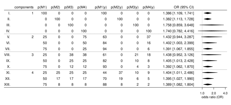
Figure 4: Analyses of the migraine data using different prior weights $p(M_{i})$ (in percent) for the model components ($M_{1}$ = “complete pooling”, $M_{2}$ = “effect-only pooling”, $M_{3}$ = “heterogeneity-only pooling”, $M_{4}$ = “standalone analyses”). The resulting posterior model probabilities $p(M_{i}|y)$ as well as corresponding estimate and CI of the OR are shown.

3.4 Sensitivity analyses

3.4.1 Varying model probabilities

We may now also investigate the effect of changing the prior probability $p(M_{1})$ expressing the a priori expectations of whether and how the two data sources may be aggregated. Fig. 3 (left panel) illustrates the resulting effect estimates (log-OR) and credible intervals when varying the prior probability $p(M_{1})$. In the extreme cases of $p(M_{1})\!=\!1$ and $p(M_{1})\!=\!0$, we are left with the simple models of “complete pooling” ($M_{1}$) and two separate “standalone analyses” ($M_{4}$), respectively. In between, we can see how the estimate is more or less “shrunk” towards the pooled estimate, and as long as $p(M_{1})\!\geq\!0.5$, the credible interval indicates a positive treatment effect.

3.4.2 Varying the vague prior specification

Besides varying the models’ prior weight via $p(M_{1})$, we can also investigate the effect of different specifications of the effect’s prior standard deviation (as defined in Sec. 2.4.3) by varying it from its initial value of $2$. Fig. 3 (right panel) illustrates the effect on the log-OR estimate and credible interval. As expected, a very small standard deviation eventually shrinks the estimate towards the prior mean (left side). For very large variances, one can see the effect of Lindley’s paradox (see Sec. 2.3): the marginal likelihood of the paediatric data under $M_{4}$ decreases, and the “pooling” component $M_{1}$ dominates the posterior.

The current setting of a standard deviation of $2$ corresponds to a priori 95% probability roughly within a range of odds ratios between $\frac{1}{50}$ and $50$. Varying the range of ORs by a factor of two ($25$ or $100$ instead of $50$) would correspond to prior standard deviations of $1.64$ or $2.35$, respectively. Doubling the standard deviation to a value of $2$ would correspond to an increase of the prior range up to values of $50^{2}\!=\!2500$ already, so the range of plausible values is probably not too far from $2$.

3.4.3 Considering more than two components

One may consider more than two components in the model, in order to account for the possibility of a different association between adolescents’ and children’s data. Fig. 4 presents the resulting estimates for a range of models with only a single or up to four components. The first columns show the prior and resulting posterior probabilities ($p(M_{i})$ and $p(M_{i}|y)$) for the different model components. Row VI shows the results discussed in Sec 3.3, while rows I, IV, V and VII are among the estimates also shown in Fig. 3 (left panel).

One can see that the results based on parameter models $M_{1}$ and $M_{2}$ as well as those for $M_{3}$ and $M_{4}$ (first four rows) are very similar. Based on the given data, it seems hard to distinguish between these pairs of models; when given equal prior probabilities, the posterior probabilities tend to be similar as well, as one can see e.g. in row XI; using only components $M_{1}$ and $M_{4}$ instead leads to a very similar estimate (row VI). Again, as soon as $p(M_{1})\!\geq\!0.5$, all credible intervals indicate a positive effect estimate.

4 Paediatric transplantation case study

4.1 Background

The data considered in the following example are from Goralczyk et al.⁴⁵ and Crins et al.⁴⁶, and these illustrate a case of an apparent prior/data conflict. Both studies were meta-analyses investigating the effect of Interleukin-2 receptor antagonists (IL-2RA) on the reported frequencies of acute rejection (AR) reactions after liver transplantation. Both reviews included controlled studies; here we focus on the subset of randomized controlled trials. The earlier publication ⁴⁵ was concerned with adults, while the more recent publication ⁴⁶ was on paediatric patients. Tab. 4 in the Appendix shows the relevant data (numbers of cases and events, and derived ORs) of 16 randomized studies; the effect sizes are also illustrated in Fig. 5. Considering the case of paediatric liver transplantation, there are only two studies available. Given the present body of evidence based on adult patients (14 studies), where the immune reaction may be similar, it is of interest to allow for this additional data to possibly inform the meta-analysis of the two paediatric studies.

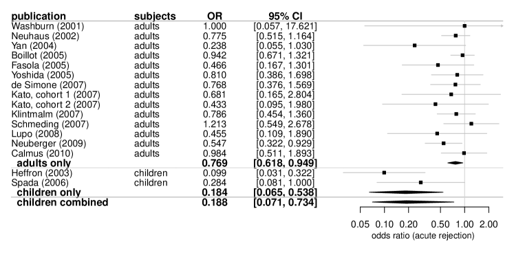
Figure 5: Forest plot for the transplantation data discussed in Sec. 4. The last two studies (Heffron (2003) and Spada (2006)) are the paediatric ones that are in the focus of the investigation, while the top 14 studies are based on adults and constitute the external information that may (potentially) be extrapolated. The endpoint of interest here is the number of acute rejection events. The combined estimate here is based on the 2-component model with $p(M_{1})=0.5$.

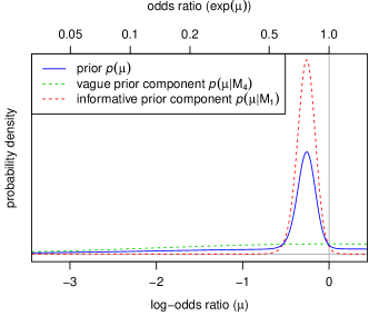
Figure 6: Prior (left) and posterior (right) densities for the example from Sec. 4. The left panel shows the prior along with its two (informative and vague) mixture components. The right panel shows the posterior, which again is a mixture of two (conditional) posteriors. The shaded area indicates the posterior 95% CI.

4.2 Analysis setup and results

We use an analogous setup as in the previous analysis and consider the two models $M_{1}$ and $M_{4}$. The prior used to analyze the paediatric data again is a heavy-tailed mixture of a vague component (as described in Sec. 3.2) and the posterior derived from the adult data. The weight of the informative prior component again is taken to be $p(M_{1})=0.5$. From the adults’ data alone we get posterior mean and standard deviation for $\mu$ of -0.266 and 0.109, respectively; the estimate and 95% CI for the OR is 0.769 [0.618, 0.949]. The resulting prior as well as conditional and marginal posteriors are illustrated in Fig. 6. The circumstances here differ from the previous example, as the paediatric data now look rather different from the external source data: we observe a larger effect (greater reduction of rejection reactions) in children than in adults (see Fig. 5).

Figure 7: Diagnostic plot showing the effect of varying the prior probability $p(M_{1})$ on the resulting effect estimate (posterior median and CI) in the transplantation example from Sec. 4.

Although a priori we would tend to assume that we might also analyse the data jointly ($p(M_{1})=0.5$), the data lead us to revise our view ($p(M_{1}|y)=0.031$); the Bayes factor here is at 30.9 in favour of the “standalone analysis” model ($M_{4}$). Fig. 7 illustrates the effect of varying the prior certainty $p(M_{1})$: one can see that the “pooling” model ($M_{1}$) is heavily discounted unless one had a very strong prior in its favour (say, $p(M_{1})>95\%$). Including the possibility of $M_{1}$ here mostly has the effect of widening the posterior to include the range suggested by the external data, and only an extremely strong prior confidence will actually shrink the posterior towards complete pooling. Effectively this leads to more cautious conclusions, including the possibility of a less pronouced effect as suggested by the external information. Based on this analysis we get an estimate and 95% CI for the OR in children of 0.188 [0.071, 0.734].

Table 1: The parameter values used in the four simulation scenarios ($S_{1}$–$S_{4}$, corresponding to models $M_{1}$–$M_{4}$) discussed in Sec. 5. The boldface figures indicate the parameters that differ between source and target.

		source		target
		parameters		parameters
scenario	(model)	$\mu_{\mathrm{S}}$	$\tau_{\mathrm{S}}$	$\mu_{\mathrm{T}}$	$\tau_{\mathrm{T}}$
$S_{1}$	($M_{1}$)	0.25	0.2	0.25	0.2
$S_{2}$	($M_{2}$)	0.25	0.2	0.25	0.5
$S_{3}$	($M_{3}$)	0.25	0.2	1.0	0.2
$S_{4}$	($M_{4}$)	0.25	0.2	1.0	0.5

Table 2: Coverage (%), and CI width in the four simulation scenarios ($S_{1}$–$S_{4}$) and using a number of analysis settings (differing numbers of studies as well as differing prior settings; similar to Fig. 4).

# studies		prior $p(M_{i})$ (%)				$S_{1}$		$S_{2}$		$S_{3}$		$S_{4}$
($k_{\mathrm{S}}+k_{\mathrm{T}}$)		$M_{1}$	$M_{2}$	$M_{3}$	$M_{4}$	coverage	width	coverage	width	coverage	width	coverage	width
$10+3$	I.	100	0	0	0	97.1	(0.66)	96.0	(0.69)	10.8	(0.73)	15.6	(0.77)
	IV.	0	0	0	100	98.7	(1.59)	95.0	(1.67)	98.7	(1.59)	94.5	(1.67)
	V.	25	0	0	75	99.6	(1.29)	97.5	(1.41)	95.4	(1.53)	89.7	(1.59)
	VI.	50	0	0	50	99.5	(1.06)	97.9	(1.19)	89.5	(1.45)	81.9	(1.50)
	VII.	75	0	0	25	98.8	(0.86)	97.9	(0.98)	76.4	(1.33)	70.4	(1.38)
	VIII.	25	0	38	38	99.3	(1.25)	96.8	(1.35)	94.8	(1.47)	88.1	(1.52)
	IX.	50	0	25	25	99.4	(1.04)	97.6	(1.16)	89.0	(1.41)	80.5	(1.45)
	X.	75	0	12	12	98.8	(0.85)	97.7	(0.97)	76.2	(1.31)	69.2	(1.35)
	XI.	25	25	25	25	99.5	(1.05)	98.3	(1.15)	89.3	(1.44)	80.5	(1.48)
	XII.	50	17	17	17	99.0	(0.92)	98.0	(1.03)	81.7	(1.37)	73.7	(1.40)
	XIII.	75	8	8	8	98.5	(0.79)	97.6	(0.89)	68.6	(1.26)	63.3	(1.30)
$3+3$	I.	100	0	0	0	98.1	(1.06)	96.2	(1.12)	77.5	(1.16)	74.9	(1.22)
	IV.	0	0	0	100	98.7	(1.59)	95.0	(1.67)	98.7	(1.59)	94.5	(1.67)
	V.	25	0	0	75	99.1	(1.42)	96.6	(1.51)	97.3	(1.54)	92.8	(1.61)
	VI.	50	0	0	50	99.1	(1.29)	96.8	(1.38)	95.2	(1.49)	90.0	(1.56)
	VII.	75	0	0	25	98.7	(1.18)	96.7	(1.27)	91.2	(1.42)	86.2	(1.48)
	VIII.	25	0	38	38	99.0	(1.40)	96.2	(1.49)	97.1	(1.52)	92.4	(1.59)
	IX.	50	0	25	25	99.0	(1.28)	96.7	(1.37)	95.0	(1.48)	89.8	(1.54)
	X.	75	0	12	12	98.7	(1.18)	96.7	(1.26)	91.2	(1.41)	86.0	(1.47)
	XI.	25	25	25	25	99.1	(1.28)	96.9	(1.36)	95.0	(1.49)	89.7	(1.55)
	XII.	50	17	17	17	98.9	(1.21)	96.8	(1.30)	92.6	(1.44)	87.3	(1.50)
	XIII.	75	8	8	8	98.6	(1.14)	96.6	(1.22)	89.1	(1.38)	84.1	(1.44)

5 Simulation study

5.1 Simulation setup

In order to gain more insight into the behaviour of the extrapolation model, we run simulations reflecting the four parameter models considered. We use three or ten ($k_{\mathrm{S}}\in\{3,10\}$) source studies with $\mu_{\mathrm{S}}\!=\!0.25$ and $\tau_{\mathrm{S}}\!=\!0.2$. Of primary interest are three ($k_{\mathrm{T}}\!=\!3$) target studies with equal or different parameters $\mu_{\mathrm{T}}$ and $\tau_{\mathrm{T}}$ as shown in Tab. 1. Estimates $y_{i}$ are generated (according to the model, see Sec. 2.1) on a continuous scale, and standard errors ($s_{i}$) are drawn uniformly between 0.2 and 1.0; for binary (log-OR) outcomes, this roughly corresponds to sample sizes between 16 and 400. We then investigate resulting coverages and mean widths of 95% CIs based on $10\,000$ replications each for each scenario, yielding a simulation error of 0.22 percentage points for the coverages.

In order to check validity of our computations, we also generated data sets with parameters drawn from the prior distribution and checked for proper coverage of the resulting credible intervals, which should be exact by construction ⁴⁷, ⁴⁸. Data were generated based on parameters drawn from the vague prior distribution, either independently or identically for target and source data with probability $0.5$, corresponding to the setting used e.g. in Sec. 3.2.

5.2 Simulation results

CI coverages and widths for $k_{\mathrm{S}}\!=\!10$ source studies are shown in Tab. 2. As expected, “naïve” extrapolation based only on model $M_{1}$ fails especially in scenarios $S_{3}$ and $S_{4}$ (row I), while a standalone analysis of the target data only yields proper coverage, but at the cost of much wider CIs (model $M_{4}$, row IV). Combining several prior components to a mixture then allows to gain in CI width, while coverage probability is slightly reduced in case of a prior/data (source/target) conflict. Again, we know that on average over the corresponding prior distribution, the coverage will be at exactly 95% by construction. Coverage is above the nominal 95% in scenario $S_{1}$ as well as the very similar $S_{2}$, and it is lower in scenarios $S_{3}$ and $S_{4}$. As already apparent in the example application in Sec. 3, due to the limited amount of data considered, models $M_{1}$ and $M_{2}$ as well as models $M_{3}$ and $M_{4}$ are barely distinguishable. Tab. 5 (see Appendix) shows that (e.g. in row XI), when the pairs of models have equal prior probabilities, the resulting posterior probabilities tend to be very similar as well, i.e., the corresponding Bayes factors are close to unity. The model similarity is also evident in the resulting estimates when comparing e.g. rows VI, IX and XI in Tab. 2 or Fig. 4.

In addition to the simulations with $k_{\mathrm{S}}\!=\!10$ “source” studies, we also investigated the performance for a smaller external evidence base of only $k_{\mathrm{S}}=3$ studies. The behaviour with respect to CI coverage and length is qualitatively similar, but not quite as pronounced. Regarding the posterior probabilities $p(M_{i}|y)$ (Tab. 5 in the Appendix) it is apparent that these are mostly determined by the prior probabilities and less affected by the data. Based on the little data only, the models apparently are hardly distinguishable, and consequently extra care should be taken to specify priors reasonably.

In the $10\,000$ simulations with parameter values drawn from the 2-component mixture prior, 94.96% of credible intervals covered the true parameter values in the setting of $k_{\mathrm{S}}\!+\!k_{\mathrm{T}}=10+3$ studies, and coverage was at 95.08% for $k_{\mathrm{S}}\!+\!k_{\mathrm{T}}=3+3$ studies, which in both cases is within the range expected for a nominal 95% coverage. This was expected by construction of the CI, as mentioned above.

6 Discussion

Mixture priors provide a means to support an analysis using external information in a robust manner ²⁴. We have showcased in two examples how the approach may easily be implemented in evidence synthesis by utilizing the simplicity of the mixture model, which implies that the posterior again constitutes a model average, a weighted mixture of the conditional posteriors based on the prior components. In the meta-analysis context, this means that off-the-shelf software may be used to perform the main computations, which then only need to be re-combined. MCMC methods only become necessary when a 4-component model is desired. The resulting procedure provides a transparent and robust data-driven approach to analysis that has the potential to either boost or discount relevant prior information, depending on its apparent compatibility.

The examples discussed here were intentionally restricted to simple random-effects meta-analysis with log-odds ratio endpoints. The same approach is readily extended to other types of endpoints that are conventionally analyzed using a random-effects model. The main point here was primarily to demonstrate the approach of using heavy-tailed ²³ or mixture priors ²⁴, its simplicity and its potential. More generally, the approach demonstrated here shows a way of overcoming the bayesmeta package’s restriction to normal effect priors, which is due to the semi-analytic implementation ^{40, 49}. Robust priors for the heterogeneity parameter may already be implemented by simply using e.g. heavy-tailed half-Student-$t$, half-Cauchy, or Lomax distributions.

When looking for example at the meta-analyses published in the Cochrane library, a large number of investigations include additional analyses of pre-defined subgroups of studies in addition to an overall estimate ⁴¹. Such cases are examples in which there may be a benefit from borrowing of information on effect or heterogeneity. The obvious danger here is that, being presented with subgroup as well as overall estimates, the practitioner may effectively perform the extrapolation in a rather intransparent manner based on eyeballing data and estimates.

While the use of two prior components may often be reasonable and sufficient, the setup has the disadvantage that prior/data conflict is confounded for effect and heterogeneity. Extending to more general formulations including more components may provide some more flexibility, if desired. However, the simulations showed that slight model variations may not be distinguishable or may not make a noticeable difference if data are sparse. Based on the principle of parsimony (Occam’s razor), one may then want to give preference to simpler, sparser model formulations.

In a Bayesian analysis, proper coverage of credible intervals is, by construction, guaranteed conditional on the prior distribution; this implies that the long-run coverage will be exact if the data-generating parameter values are repeatedly drawn from the prior distribution⁴⁸. However, coverage probability is not necessarily at the nominal level when data are generated repeatedly based on single constant parameter values (which is the common frequentist requirement⁵⁰). By constructing the prior as informative, and complementing the informative prior with a “robustifying” vague component, we expect the coverage to exceed the nominal credible level when conditioning on the informative component only, and to be lower conditional on the vague component. As usual, inferences will be reasonable and consistent when model and prior are specified sensibly; in the present case it is especially crucial to also specify the vague prior component realistically. In contrast to immediate intuition, a larger prior variance is not necessarily a more conservative choice, due to Lindley’s paradox. In order to enhance robustness, the prior probability of the vague component should be increased instead.

Many other variations of the approach are conceivable. The external information does not necessarily need to come from a second meta-analysis, but could also be based on other types of data. Likewise, the “main” analysis does not need to be a meta-analysis, but could also be a single study with a meta-analysis informing the prior, which would lead to an approach very similar to the original setup discussed by Schmidli et al.²⁴.

The presented approach however is no substitute for a careful check of appropriateness of possible data pooling. Note that in the transplantation example a joint analysis may already be highly questionable on theoretical grounds. While in the preceding migraine example, it is conceivable that with adjusted dosing a comparable effect may be achieved in adolescents and children, in the transplantation context, indications and surgical practice differ between adults and children in a range of aspects, so that a similarity of effect may already be doubtful a priori. Even if the different data themselves may not be obviously contradicting, pooling always also requires a theoretical justification, and plausibility should be reflected in the model setup (here especially in the weighting of prior components).

Appendix A Mixture posterior derivation

Consider a setup where the prior distribution is a two-component mixture

$$p(\vartheta)\;=\;p(\vartheta|M_{a})\,p(M_{a})+p(\vartheta|M_{b})\,p(M_{b})$$ (8)

and interest lies in determining the posterior $p(\vartheta|y)$ based on data $y$ and some likelihood function $p(y|\vartheta)$. The parameters’ posterior distribution then is given by

$$p(\vartheta|y)\;=\;\frac{p(y|\vartheta)\;p(\vartheta)}{\int p(y|\vartheta)\,p(\vartheta)\,\mathrm{d}\vartheta}$$ (9)

$$= \frac{p(y|\vartheta)\;\bigl{(}p(\vartheta|M_{a})\,p(M_{a})+p(\vartheta|M_{b})\,p(M_{b})\bigr{)}}{\int p(y|\vartheta)\,\bigl{(}p(\vartheta|M_{a})\,p(M_{a})+p(\vartheta|M_{b})\,p(M_{b})\bigr{)}\,\mathrm{d}\vartheta}$$ (10)

$$= \frac{p(M_{a})\,p(y|\vartheta)\,p(\vartheta|M_{a})+p(M_{b})\,p(y|\vartheta)\,p(\vartheta|M_{b})}{p(M_{a})\,\int p(y|\vartheta)\,p(\vartheta|M_{a})\,\mathrm{d}\vartheta+p(M_{b})\,\int p(y|\vartheta)\,p(\vartheta|M_{b})\,\mathrm{d}\vartheta}$$ (11)

$$= \frac{p(M_{a})\,p(y|\vartheta)\,p(\vartheta|M_{a})+p(M_{b})\,p(y|\vartheta)\,p(\vartheta|M_{b})}{p(M_{a})\,p(y|M_{a})+p(M_{b})\,p(y|M_{b})}$$ (12)

$$= \frac{p(M_{a})\,p(y|\vartheta)\,p(\vartheta|M_{a})}{p(M_{a})\,p(y|M_{a})+p(M_{b})\,p(y|M_{b})}$$ (15)

$$+\frac{p(M_{b})\,p(y|\vartheta)\,p(\vartheta|M_{b})}{p(M_{a})\,p(y|M_{a})+p(M_{b})\,p(y|M_{b})}$$

$$= \frac{p(y|\vartheta)\;p(\vartheta|M_{a})}{p(y|M_{a})}\;\frac{p(M_{a})\,p(y|M_{a})}{p(M_{a})\,p(y|M_{a})+p(M_{b})\,p(y|M_{b})}$$

$$+\frac{p(y|\vartheta)\;p(\vartheta|M_{b})}{p(y|M_{b})}\;\frac{p(M_{b})\,p(y|M_{b})}{p(M_{a})\,p(y|M_{a})+p(M_{b})\,p(y|M_{b})}$$

$$= p(\vartheta|y,M_{a})\;p(M_{a}|y)+p(\vartheta|y,M_{b})\;p(M_{b}|y)\mbox{,}$$ (16)

which again is a mixture of the two conditional posterior distributions $p(\vartheta|y,M_{a})$ and $p(\vartheta|y,M_{b})$.

Appendix B Example data

Tab. 3 shows the paediatric migraine example data due to Richer et al.⁴³, which are discussed in Sec. 3. The paediatric transplantation example data due to Crins et al.⁴⁶, which are used in Sec. 4, are shown in Tab. 4.

Table 3: Data set due to Richer et al.⁴³; the numbers of events and total numbers of patients in treatment and control groups are shown along with the corresponding derived logarithmic odds ratios (log-ORs) and confidence intervals.

	patient	triptan	placebo	log-OR
publication	type	group	group	(95% CI)
Hämäläinen (1997b)	adolescents	7 / 23	5 / 23	0.454 [-0.876, 1.785]
Rothner (1997)	adolescents	113 / 226	46 / 74	-0.496 [-1.034, 0.041]
Winner (1997)	adolescents	111 / 222	32 / 76	0.318 [-0.207, 0.844]
Rothner (1999a)	adolescents	96 / 186	20 / 34	-0.292 [-1.033, 0.449]
Rothner (1999b)	adolescents	17 / 62	7 / 30	0.216 [-0.797, 1.230]
Rothner (1999c)	adolescents	23 / 66	14 / 36	-0.174 [-1.014, 0.666]
Winner (2000)	adolescents	243 / 377	69 / 130	0.472 [0.068, 0.876]
Winner (2002)	adolescents	98 / 149	80 / 142	0.398 [-0.076, 0.872]
Ahonen (2004)	adolescents	53 / 83	32 / 83	1.035 [0.406, 1.664]
Visser (2004a)	adolescents	159 / 233	165 / 240	-0.024 [-0.412, 0.364]
Ahonen (2006)	adolescents	71 / 96	35 / 96	1.599 [0.982, 2.216]
Evers (2006)	adolescents	18 / 29	8 / 29	1.458 [0.350, 2.565]
Rothner (2006)	adolescents	262 / 480	93 / 160	-0.144 [-0.506, 0.218]
Winner (2006)	adolescents	316 / 483	141 / 242	0.304 [-0.013, 0.621]
Callenbach (2007)	adolescents	19 / 46	15 / 46	0.375 [-0.477, 1.226]
Lewis (2007)	adolescents	97 / 148	67 / 127	0.533 [0.046, 1.019]
Winner (2007)	adolescents	82 / 144	79 / 133	-0.101 [-0.579, 0.377]
Linder (2008)	adolescents	383 / 544	94 / 170	0.654 [0.300, 1.008]
Ho (2012)	adolescents	167 / 284	147 / 286	0.300 [-0.031, 0.631]
Fujita (2014)	adolescents	23 / 74	27 / 70	-0.331 [-1.019, 0.357]
Ueberall (1999)	children	12 / 14	6 / 14	2.079 [0.246, 3.913]
Hämäläinen (2002)	children	38 / 59	24 / 58	0.941 [0.195, 1.688]
Ho (2012)	children	53 / 98	57 / 102	-0.073 [-0.630, 0.485]

Table 4: Data set due to Goralczyk et al.⁴⁵ and Crins et al.⁴⁶. The numbers of events and total numbers of patients in treatment and control groups are shown along with the corresponding derived odds ratios (ORs) and confidence intervals.

	patient	IL-2RA	control	odds ratio
publication	type	group	group	(95% CI)
Washburn (2001)	adults	1 / 15	1 / 15	1.000 [0.057, 17.62]
Neuhaus (2002)	adults	74 / 188	88 / 193	0.775 [0.515, 1.164]
Yan (2004)	adults	3 / 24	9 / 24	0.238 [0.055, 1.030]
Boillot (2005)	adults	89 / 351	92 / 347	0.942 [0.671, 1.321]
Fasola (2005)	adults	13 / 46	11 / 24	0.466 [0.167, 1.301]
Yoshida (2005)	adults	17 / 72	21 / 76	0.810 [0.386, 1.698]
de Simone (2007)	adults	17 / 95	21 / 95	0.768 [0.376, 1.569]
Kato, cohort 1 (2007)	adults	7 / 15	9 / 16	0.681 [0.165, 2.804]
Kato, cohort 2 (2007)	adults	3 / 16	8 / 23	0.433 [0.095, 1.980]
Klintmalm (2007)	adults	80 / 153	46 / 79	0.786 [0.454, 1.360]
Schmeding (2007)	adults	29 / 51	25 / 48	1.213 [0.549, 2.678]
Lupo (2008)	adults	4 / 26	6 / 21	0.455 [0.109, 1.890]
Neuberger (2009)	adults	28 / 168	45 / 168	0.547 [0.322, 0.929]
Calmus (2010)	adults	23 / 98	24 / 101	0.984 [0.511, 1.893]
Heffron (2003)	children	14 / 61	15 / 20	0.099 [0.031, 0.322]
Spada (2006)	children	4 / 36	11 / 36	0.284 [0.081, 1.000]

Appendix C Additional simulation results: model proabilities

Tab. 5 below shows the average model probabilities corresponding to the simulation results shown in Tab. 2 (Sec. 5).

Table 5: Average posterior model probabilities $p(M_{i}|y)$ (in %) in the four simulation scenarios ($S_{1}$–$S_{4}$).

# studies		prior $p(M_{i})$ (%)				$S_{1}$				$S_{2}$				$S_{3}$				$S_{4}$
($k_{\mathrm{S}}+k_{\mathrm{T}}$)		$M_{1}$	$M_{2}$	$M_{3}$	$M_{4}$	$\quad M_{1}$	$M_{2}$	$M_{3}$	$M_{4}$	$\quad M_{1}$	$M_{2}$	$M_{3}$	$M_{4}$	$\quad M_{1}$	$M_{2}$	$M_{3}$	$M_{4}$	$\quad M_{1}$	$M_{2}$	$M_{3}$	$M_{4}$
$10+3$	V.	25	0	0	75	55	0	0	45	48	0	0	52	27	0	0	73	27	0	0	73
	VI.	50	0	0	50	77	0	0	23	70	0	0	30	46	0	0	54	45	0	0	55
	VII.	75	0	0	25	90	0	0	10	86	0	0	14	65	0	0	35	62	0	0	38
	VIII.	25	0	38	38	54	0	23	23	48	0	25	27	27	0	38	36	27	0	36	37
	IX.	50	0	25	25	76	0	12	12	70	0	14	15	46	0	28	27	45	0	27	28
	X.	75	0	12	12	90	0	5	5	86	0	7	7	64	0	18	17	62	0	18	19
	XI.	25	25	25	25	39	37	12	12	35	36	14	14	23	24	27	26	22	25	26	26
	XII.	50	17	17	17	65	20	7	7	60	21	9	9	43	16	21	20	41	17	21	21
	XIII.	75	8	8	8	85	9	3	3	81	10	5	5	64	8	14	13	62	9	15	15
$3+3$	V.	25	0	0	75	48	0	0	52	45	0	0	55	32	0	0	68	31	0	0	69
	VI.	50	0	0	50	72	0	0	28	69	0	0	31	53	0	0	47	52	0	0	48
	VII.	75	0	0	25	88	0	0	12	86	0	0	14	73	0	0	27	71	0	0	29
	VIII.	25	0	38	38	48	0	26	26	45	0	27	28	31	0	35	34	31	0	34	35
	IX.	50	0	25	25	72	0	14	14	69	0	15	16	53	0	24	23	52	0	24	24
	X.	75	0	12	12	88	0	6	6	86	0	7	7	72	0	14	14	71	0	14	14
	XI.	25	25	25	25	37	35	14	14	35	35	15	15	26	27	23	23	26	27	23	24
	XII.	50	17	17	17	63	20	8	8	60	20	10	10	49	17	17	17	48	17	17	17
	XIII.	75	8	8	8	83	9	4	4	81	9	5	5	71	8	10	10	70	8	11	11

Appendix D Example R code

D.1 Two-component mixture

The following R code allows to reproduce the analysis from Sec. 3. In addition to R ²⁷, the metafor ⁵¹ and bayesmeta ^{28, 40} packages are required. The other analyses are done completely analogously.

# read data:
RicherEtAl2016 <- read.csv("RicherEtAl2016.csv",
                           colClasses=c("study"="character"))
# compute effect sizes (log-ORs):
require("metafor")
effsize <- escalc(measure="OR",
                  ai=triptan.events, n1i=triptan.total,
                  ci=placebo.events, n2i=placebo.total,
                  slab=study, data=RicherEtAl2016)
# specify subset indices:
aidx <- (effsize[,"patients"]=="adolescents")
cidx <- (effsize[,"patients"]=="children")


########################
# main MA computations:
require("bayesmeta")

# standard deviation of vague prior:
vaguepriorsd <- 2

# meta analysis for adolescents only:
bma.adol <- bayesmeta(effsize[aidx,],
              mu.prior.mean=0, mu.prior.sd=vaguepriorsd,
              tau.prior=function(t){dhalfnormal(t,scale=0.5)})

# meta analysis for children only:
bma.child <- bayesmeta(effsize[cidx,],
               mu.prior.mean=0, mu.prior.sd=vaguepriorsd,
               tau.prior=function(t){dhalfnormal(t,scale=0.5)})

# joint meta analysis for all patients:
bma.joint <- bayesmeta(effsize,
               mu.prior.mean=0, mu.prior.sd=vaguepriorsd,
               tau.prior=function(t){dhalfnormal(t,scale=0.5)})

# assemble marginal likelihoods:
marginals <- c("M1: pooled"   = bma.joint$marginal,
               "M4: separate" = bma.adol$marginal
                                * bma.child$marginal)
print(marginals)
barplot(marginals, ylab="marginal likelihood")

# Bayes factor:
bf <- marginals[1] / marginals[2]
print(c("M1: pooled"=unname(bf), "M4: separate"=1/unname(bf)))

# specify prior (p(M1)):
prior.prob <- 0.50
prior.odds <- prior.prob / (1-prior.prob)

# determine posterior:
post.odds <- prior.odds * bf
post.prob <- post.odds / (post.odds+1)
print(post.prob)

# show prior & posterior probabilities:
print(matrix(c(prior.prob, 1-prior.prob,
               post.prob, 1-post.prob),
             nrow=2, ncol=2, byrow=TRUE,
             dimnames=list(c("prior","posterior"),
                           c("M1: pooled","M4: separate"))))


##############################################################
# functions to compute cumulative distribution function etc.:

# cumulative distribution function (CDF):
cdf <- function(mu=0, prob = post.prob)
{
  dens <- function(x)
  {
    return(prob*bma.joint$dposterior(mu=x)
           + (1-prob)*bma.child$dposterior(mu=x))
  }
  integral <- integrate(dens, lower=-Inf, upper=mu)
  return(integral$value)
}

# quantile function (inverse CDF):
invcdf <- function(p, xrange=c(-4,4), prob=post.prob)
{
  if ((cdf(xrange[1], prob=prob)<p)&(cdf(xrange[2], prob=prob)>p))
    result <- uniroot(function(x){cdf(x, prob=prob)-p},
                      lower=xrange[1], upper=xrange[2])$root
  else
    result <- NA
  return(result)
}

# function to determine shortest credible interval:
shortest.interval <- function(level=0.95,
                              min.p=0.001, prob=post.prob)
{
  intwidth <- function(left)
  {
    pleft <- cdf(left, prob=prob)
    right <- invcdf(level+pleft, prob=prob)
    return(right-left)
  }
  opti <- optimize(intwidth, lower=invcdf(min.p, prob=prob),
                   upper=invcdf(1-level, prob=prob))$minimum
  result <- c(opti, invcdf(level+cdf(opti, prob=prob), prob=prob))
  return(result)
}


########################################################
# compute eventual estimates (median and 95% interval):

# median & credible interval:
esti <- c("median" = invcdf(0.5, prob=post.prob),
          "lower" = NA, "upper" = NA)
# shortest interval:
esti[2:3] <- shortest.interval(prob=post.prob)
print(esti)
print(exp(esti))

D.2 Three-component mixture

The following R code allows to reproduce the analysis shown in row IX. of Fig. 4, using a 3-component mixture for the prior.

# read data:
RicherEtAl2016 <- read.csv("RicherEtAl2016.csv",
                           colClasses=c("study"="character"))
# compute effect sizes (log-ORs):
require("metafor")
effsize <- escalc(measure="OR",
                  ai=triptan.events, n1i=triptan.total,
                  ci=placebo.events, n2i=placebo.total,
                  slab=study, data=RicherEtAl2016)
# subset indices:
aidx <- (effsize[,"patients"]=="adolescents")
cidx <- (effsize[,"patients"]=="children")

########################
# main MA computations:
require("bayesmeta")

# standard deviation of vague prior:
vaguepriorsd <- 2

# meta analysis for adolescents only:
bma.adol <- bayesmeta(effsize[aidx,],
              mu.prior.mean=0, mu.prior.sd=vaguepriorsd,
              tau.prior=function(t){dhalfnormal(t,scale=0.5)})

# meta analysis for children only:
bma.child <- bayesmeta(effsize[cidx,],
               mu.prior.mean=0, mu.prior.sd=vaguepriorsd,
               tau.prior=function(t){dhalfnormal(t,scale=0.5)})

# joint meta analysis (BOTH parameters) for all patients:
bma.joint <- bayesmeta(effsize,
               mu.prior.mean=0, mu.prior.sd=vaguepriorsd,
               tau.prior=function(t){dhalfnormal(t,scale=0.5)})

# meta analysis for children only,
# heterogeneity prior from adolescents:
bma.child.t <- bayesmeta(effsize[cidx,],
                mu.prior.mean=0, mu.prior.sd=vaguepriorsd,
                tau.prior=function(t){bma.adol$dposterior(tau=t)})


# show some results
# (adolescents only / pooled / pooling tau only / children):
rbind("adolescents"=bma.adol$summary[,"mu"],
      "M1: pooled"=bma.joint$summary[,"mu"],
      "M3: pooled (tau only)"=bma.child.t$summary[,"mu"],
      "M4: separate"=bma.child$summary[,"mu"])


# assemble marginal likelihoods:
marginals <- c("M1: pooled (mu+tau)"   = bma.joint$marginal,
               "M3: pooled (tau only)" = bma.adol$marginal
                                         * bma.child.t$marginal,
               "M4: separate"          = bma.adol$marginal
                                         * bma.child$marginal)
print(marginals)
barplot(marginals, ylab="marginal likelihood")

# specify prior:
prior.prob <- c("M1: pooled (mu+tau)"   = 1/2,
                "M3: pooled (tau only)" = 1/4,
                "M4: separate"          = 1/4)

# determine posterior:
post.prob <- prior.prob * marginals
post.prob <- post.prob / sum(post.prob)

# show prior & posterior probabilities:
print(round(rbind("prior"=prior.prob, "posterior"=post.prob),3))


##############################################################
# functions to compute cumulative distribution function etc.:

# cumulative distribution function (CDF):
cdf <- function(mu=0, prob = post.prob)
{
  stopifnot(length(prob)==3, all(is.finite(prob)),
            all(prob>=0), all(prob<=1), sum(prob)==1)
  dens <- function(x)
  {
    return(prob[1]*bma.joint$dposterior(mu=x)
           + prob[2]*bma.child.t$dposterior(mu=x)
           + prob[3]*bma.child$dposterior(mu=x))
  }
  integral <- integrate(dens, lower=-Inf, upper=mu)
  return(integral$value)
}

# quantile function (inverse CDF):
invcdf <- function(p, xrange=c(-4,4), prob=post.prob)
{
  if ((cdf(xrange[1], prob=prob)<p)&(cdf(xrange[2], prob=prob)>p))
    result <- uniroot(function(x){cdf(x, prob=prob)-p},
                      lower=xrange[1], upper=xrange[2])$root
  else
    result <- NA
  return(result)
}

# function to determine shortest credible interval:
shortest.interval <- function(level=0.95,
                              min.p=0.001, prob=post.prob)
{
  intwidth <- function(left)
  {
    pleft <- cdf(left, prob=prob)
    right <- invcdf(level+pleft, prob=prob)
    return(right-left)
  }
  opti <- optimize(intwidth, lower=invcdf(min.p, prob=prob),
                   upper=invcdf(1-level, prob=prob))$minimum
  result <- c(opti, invcdf(level+cdf(opti, prob=prob), prob=prob))
  return(result)
}


########################################################
# compute eventual estimates (median and 95% interval):

# median & symmetric interval:
esti <- c("median"  = invcdf(0.5, prob=post.prob),
          "lower" = NA, "upper" = NA)
# shortest interval (on log scale):
esti[2:3] <- shortest.interval(prob=post.prob)
print(esti)
print(exp(esti))

References

- 1 European Medicines Agency (EMA) . Reflection paper on extrapolation of efficacy and safety in pediatric medicine development. EMA/199678/2016; 2016.
- 2 U.S. Department of Health and Human Services, Food and Drug Administration (FDA) . Use of real-world evidence to support regulatory decision-making for medical devices. 2017.
- 3 European Medicines Agency (EMEA) . Guideline on clinical trials in small populations. CHMP/EWP/83561/2005; 2006.
- 4 U.S. Department of Health and Human Services, Food and Drug Administration (FDA) . Leveraging existing clinical data for extrapolation to pediatric uses of medical devices – Guidance for industry and Food and Drug Administration staff Draft guidance2016.
- 5 ICH . Ethnic factors in the acceptability of foreign clinical data. ICH Harmonized Tripartite Guideline E5(R1): International Conference on Harmonisation of Technical Requirements for Registration of Pharmaceuticals for Human Use; 1998.
- 6 Dunne J., others . Extrapolation of adult data and other data in pediatric drug-development programs. Pediatrics. 2011;128(5):e1242-e1249.
- 7 Jonker A. H., others . Small population clinical trials: challenges in the field of rare diseases. small population clinical trials task force workshop report and recommendations: International Rare Diseases Research Consortium (IRDiRC); 2016.
- 8 Dunoyer M.. Accelerating access to treatments for rare diseases. Nature Reviews Drug Discovery. 2011;10(7):475-476.
- 9 Hampson L. V., Whitehead J., Eleftheriou D., Brogan P.. Bayesian methods for the design and interpretation of clinical trials in very rare diseases. Statistics in Medicine. 2014;33(24):4186-4201.
- 10 Neuenschwander B., Capkun-Niggli G., Branson M., Spiegelhalter D. J.. Summarizing historical information on controls in clinical trials. Clinical Trials. 2010;7(1):5-18.
- 11 Gerß J. W. O., Köpcke W.. Clinical trials and rare diseases. In: Paz M. P., Croft S. C., eds. Rare diseases epidemiology, Springer 2010 (pp. 173-190).
- 12 Neuenschwander B., Roychoudhuri S., Schmidli H.. On the use of co-data in clinical trials. Statistics in Biopharmaceutical Research. 2016;8(3):345-354.
- 13 Wadsworth I., Hampson L. V., Jaki T.. Extrapolation of efficacy and other data to support the development of new medicines for children: A systematic review of methods. Statistical Methods in Medical Research. 2016;.
- 14 Schoenfeld D. A., Zheng H., Finkelstein D. M.. Bayesian design using adult data to augment pediatric trials. Clinical Trials. 2009;6(9):297-304.
- 15 Gamalo-Siebers M., Savic J., Basu C., others . Statistical modeling for Bayesian extrapolation of adult clinical trial informaton in pediatric drug evaluation. Pharmaceutical Statistics. 2017;16(4):232-249.
- 16 Hlavin G., Koenig F., Male C., Posch M., Bauer P.. Evidence, eminence and extrapolation. Statistics in Medicine. 2016;35(13):2117-2132.
- 17 Friede T., Röver C., Wandel S., Neuenschwander B.. Meta-analysis of few small studies in orphan diseases. Research Synthesis Methods. 2017;8(1):79-91.
- 18 Friede T., Röver C., Wandel S., Neuenschwander B.. Meta-analysis of two studies in the presence of heterogeneity with applications in rare diseases. Biometrical Journal. 2017;59(4):658-671.
- 19 Davey J., Turner R. M., Clarke M. J., Higgins J. P. T.. Characteristics of meta-analyses and their component studies in the Cochrane Database of Systematic Reviews: a cross-sectional, descriptive analysis. BMC Medical Research Methodology. 2011;11(1):160.
- 20 Turner R. M., Davey J., Clarke M. J., Thompson S. G., Higgins J. P. T.. Predicting the extent of heterogeneity in meta-analysis, using empirical data from the Cochrane Database of Systematic Reviews. International Journal of Epidemiology. 2012;41(3):818-827.
- 21 Bender R., Friede T., Koch A., et al. Methods for evidence synthesis in the case of very few studies. Research Synthesis Methods. 2018;.
- 22 Fúquene J. A., Cook J. D., Pericchi L. R.. A case for robust Bayesian priors with applications to clinical trials. Bayesian Analysis. 2009;4(4):817-846.
- 23 O’Hagan A., Pericchi L.. Bayesian heavy-tailed models and conflict resolution: A review. Brazilian Journal of Probability and Statistics. 2012;26(4):372-401.
- 24 Schmidli H., Gsteiger S., Roychoudhury S., O’Hagan A., Spiegelhalter D., Neuenschwander B.. Robust meta-analytic-predictive priors in clinical trials with historical control information. Biometrics. 2014;70(4):1023-1032.
- 25 Hoeting J. A., Madigan D., Raftery A., Volinsky C. T.. Bayesian model averaging: a tutorial. Statistical Science. 1999;14(4):382-401.
- 26 Bornkamp B., Ohlssen D., Magnusson B. P., Schmidli H.. Model averaging for treatment effect estimation in subgroups. Pharmaceutical Statistics. 2016;16(2):133-142.
- 27 R Development Core Team . R: A language and environment for statistical computing. R Foundation for Statistical ComputingVienna, Austria2016.
- 28 Röver C.. bayesmeta: Bayesian random-effects meta analysis. R package. URL: http://cran.r-project.org/package=bayesmeta; 2015.
- 29 Plummer M.. rjags: Bayesian graphical models using MCMC2008. R package.
- 30 Hedges L. V., Olkin I.. Statistical methods for meta-analysis. San Diego, CA, USA: Academic Press; 1985.
- 31 Hartung J., Knapp G., Sinha B. K.. Statistical meta-analysis with applications. Hoboken, NJ, USA: John Wiley & Sons; 2008.
- 32 Borenstein M., Hedges L. V., Higgins J. P. T., Rothstein H. R.. Introduction to Meta-Analysis. John Wiley & Sons; 2009.
- 33 Spiegelhalter D. J., Abrams K. R., Myles J. P.. Bayesian approaches to clinical trials and health-care evaluation. John Wiley & Sons; 2004.
- 34 U.S. Department of Health and Human Services, Food and Drug Administration (FDA) . Guidance for the use of Bayesian statistics in medical device clinical trials. 2010.
- 35 Hsiao C.-F., Hsu Y.-Y., Tsou H.-H.. Use of prior information for Bayesian evaluation of bridging studies. Journal of Biopharmaceutical Statistics. 2007;17(1):109-121.
- 36 Kass A. E., Raftery R. E.. Bayes Factors. Journal of the American Statistical Association. 1995;90(430):773-795.
- 37 Clemen R. T.. Combining forecasts: a review and annotated bibliography. International Journal of Forecasting. 1989;5(4):559-583.
- 38 Clyde M., George E. I.. Model uncertainty. Statistical Science. 2004;19(1):81-94.
- 39 Lindley D. V.. A statistical paradox. Biometrika. 1957;44(1/2):187-192.
- 40 Röver C.. Bayesian random-effects meta-analysis using the bayesmeta R package. arXiv preprint 1711.08683. 2017;.
- 41 Turner R. M., Jackson D., Wei Y., Thompson S. G., Higgins P. T.. Predictive distributions for between-study heterogeneity and simple methods for their application in Bayesian meta-analysis. Statistics in Medicine. 2015;34(6):984-998.
- 42 Rhodes K. M., Turner R. M., Higgins J. P. T.. Predictive distributions were developed for the extent of heterogeneity in meta-analyses of continuous outcome data. Journal of Clinical Epidemiology. 2015;68(1):52-60.
- 43 Richer L., Billinghurst L., Lisdell M. A., et al. Drugs for the acute treatment of migraine in children and adolescents. Cochrane Database of Systematic Reviews. 2016;4:CD005220.
- 44 Neuenschwander B., Wandel S., Roychoudhury S., Bailey S.. Robust exchangeability designs for early phase clinical trials with multiple strata. Pharmaceutical Statistics. 2016;15(2):123-134.
- 45 Goralczyk A. D., Hauke N., Bari N., Tsui T. Y., Lorf T., others . Interleukin-2 receptor antagonists for liver transplant recipients: A systematic review and meta-analysis of controlled studies. Hepatology. 2011;54(2):541-554.
- 46 Crins N. D., Röver C., Goralczyk A. D., Friede T.. Interleukin-2 receptor antagonists for pediatric liver transplant recipients: A systematic review and meta-analysis of controlled studies. Pediatric Transplantation. 2014;18(8):839-850.
- 47 Dawid A. P.. The well-calibrated Bayesian. Journal of the American Statistical Association. 1982;77(379):605-610.
- 48 Cook S. R., Gelman A., Rubin D. B.. Validation of software for Bayesian models using posterior quantiles. Journal of Computational and Graphical Statistics. 2006;15(3):675-692.
- 49 Röver C., Friede T.. Discrete approximation of a mixture distribution via restricted divergence. Journal of Computational and Graphical Statistics. 2017;26(1):217-222.
- 50 Neyman J., Pearson E. S.. On the problem of the most efficient tests of statistical hypotheses. Philosophical Transactions of the Royal Society of London, Series A. 1933;231:289-337.
- 51 Viechtbauer W.. Conducting meta-analyses in R with the metafor package. Journal of Statistical Software. 2010;36(3).