Numerical simulations to the Vlasov-Poisson system with a strong magnetic field

Abstract.

In this paper, we present a Particle-In-Cell algorithm based on semi-implicit/explicit time discretization techniques for the simulation of the three dimensional Vlasov-Poisson system in the presence of a strong external magnetic field. When the intensity of the magnetic field is sufficiently large and for any time step, the numerical scheme provides formally a consistent approximation of the drift-kinetic model, which corresponds to the asymptotic model. Numerical results show that this new Particle-In-Cell method is efficient and accurate for large time steps.

Francis Filbet

Institut de Mathématiques de Toulouse, UMR5219, Université de Toulouse & IUF , F-31062

Toulouse, France

Chang Yang

Department of Mathematics, Harbin Institute of Technology,

92 West Dazhi Street, Nan Gang District, Harbin 150001, China

1. Introduction

Magnetized plasmas are encountered in a wide variety of astrophysical situations, but also in magnetic fusion devices such as tokamaks, where a large external magnetic field needs to be applied in order to keep the particles on the desired tracks. Such a dynamic can be described by the Vlasov-Poisson equation, where plasma particles evolve under self-consistent electrostatic field and the confining magnetic field.

We assume that on the time scale we consider, collisions can be neglected both for ions and electrons, hence collective effects are dominant and the plasma is entirely modelled with kinetic transport equations, where the unknown is the number density of particles $f(t,\mathbf{x},\mathbf{v})$ depending on time $t\geq 0$, position $\mathbf{x}\in{\mathbb{R}}^{3}$ and velocity $\mathbf{v}\in{\mathbb{R}}^{3}$. Such a kinetic model provides an appropriate description of turbulent transport in a fairly general context, but it requires to solve a six dimensional problem which leads to a huge computational cost.

On the one hand, many asymptotic models with a smaller number of variables than the kinetic description were developed. For instance, large magnetic fields usually lead to the so-called drift-kinetic limit [19, 20, 12] and for a mathematical point of view [17, 27, 3, 4]. In this regime, due to the large applied magnetic field, particles are confined along the magnetic field lines and their period of rotation around these lines (called the cyclotron period) becomes small. However, such a reduced model only valid with strong magnetic field assumption, hence it could not describe all physics of magnetized plasma. On the other hand, in some recent work [29, 26], numerical methods are developed for the full kinetic models, such as the Vlasov-Maxwell equation. For example, in [26] and [24, 25], the authors have developed a symplectic Particle-In-Cell method, which can preserve the geometrical structure of the system, hence this property may help to preserve the accuracy for long time simulation. However, in our context, this scheme is not necessarily efficient due to its complexity and the limitation on the time step since it requires the time resolution of all time scales.

Another approach with similar advantages, developed in [6, 8, 9] and [7, 16], consists in explicitly doubling time variables and seeking higher-dimensional partial differential equations and boundary conditions in variables $(t,\tau,\mathbf{x},\mathbf{v})$ that contains the original system at the $\varepsilon$-diagonal $(t,\tau)=(t,t/\varepsilon)$ where $\varepsilon$ represents for instance the ratio between the plasma and the cyclotron frequencies. While the corresponding methods are extremely good at capturing oscillations their design require a deep a priori understanding of the detailed structure of oscillations.

In the very recent works of Filbet and Rodrigues [13, 14], a new asymptotically stable Particle-In-Cell methods are developed in the request of efficiency for full kinetic models. The numerical methods are developed in the two-dimensional framework, where one restricts to the perpendicular dynamics. On the one hand, this numerical methods contain the efficient property of the Particle-In-Cell (PIC) method; on the other hand, this numerical method is free from the stiffness of the full kinetic system. Moreover, up to third order method is also proposed, thus this method is very accurate for long term simulations.

In this paper, we extend the asymptotically stable Particle-In-Cell methods for three dimensional Vlasov-Poisson equation. For clarity, we first consider a cylindrical geometry with uniform external magnetic filed. Under this assumption, by following the main lines in [13], we develop implicit numerical methods for the characteristic curve system. More precisely, though the numerical methods are implicit, only the stiff terms (characterized by $1/\varepsilon$) are implicitly computed, and the other terms can be explicitly computed. Then by reformulating the numerical methods and dropping the second order terms with respect to $\varepsilon$, we derive the numerical methods for the characteristic curve system corresponding to the Drift-Kinetic model. We can formally show the solutions of these two systems are second order consistent with respect to $\varepsilon$.

The rest of the paper is organized as follows. In Section 2, we derive the Vlasov-Poisson equation in our interested scaling, and develop its second order consistent non-stiff model, the drift-Kinetic model. In Section 3 we present several time discretization techniques based on high-order semi-implicit schemes [2] for the Vlasov-Poisson system with a strong external magnetic field, and we prove consistency of the schemes even when the intensity of the magnetic field becomes large with preservation of the order of accuracy (from first to third order accuracy). Section 5 is then devoted to numerical simulations for one single particle motion and for the Vlasov-Poisson model for various asymptotics, which illustrate the advantage of high order schemes. Finally in Section 6, we conclude the paper and give the perspectives.

2. Mathematical models

In this section, we will introduce the models to describe the electrostatic perturbations of spatially non-uniform plasmas. The Vlasov equation for the ion distribution function $f$ in standard form in standard notation is

(2.1) $$\frac{\partial f}{\partial t}\,+\,\mathbf{v}\cdot\nabla_{\mathbf{x}}f\,+\,\frac{q}{m}\left({\mathbf{E}}+\mathbf{v}\wedge{\mathbf{B}}_{\rm ext}\right)\cdot\nabla_{\mathbf{v}}f\,=\,0,$$

where $t\in{\mathbb{R}}^{+}$ is the time variable, $\mathbf{x}\in\Omega\subset{\mathbb{R}}^{3}$ is the space variable, $\mathbf{v}\in{\mathbb{R}}^{3}$ is the velocity variable, $m$ is the ion particle mass, $q$ is its charge, ${\mathbf{E}}=-\nabla_{\mathbf{x}}\phi(t,\mathbf{x})$ is the electric field and ${\mathbf{B}}_{\rm ext}$ is the external magnetic field. The potential $\phi$ is solution to the Poisson equation

(2.2) $$-\epsilon_{0}\,\Delta_{\mathbf{x}}\phi\,=\,{\rho},$$

where $\epsilon_{0}$ represents the permittivity of vacuum and $\rho$ is the charge density

$$\rho(t,\mathbf{x})\,:=\,q\,\int_{{\mathbb{R}}^{3}}f(t,\mathbf{x},\mathbf{v})\,\textrm{d}\mathbf{v}\,-\,\rho_{0},$$

with $\rho_{0}$ the charge density of a fixed species. For practical applications, this model has to be supplemented with suitable boundary conditions. Here we will consider a cylindrical domain of the form

$$\Omega=\left\{(x,y,z)\in\mathbb{R}^{3};\,\,(x,y)\in D,\,0\,\leq\,z\,\leq\,L_{z}\right\},$$

where $D$ an arbitrary two dimensional domain (disk and D-shaped domain will be used). We assume that the electric potential is periodic in the $z$ variable and vanishes at the boundary $\partial D$

(2.3) $$\phi(\mathbf{x})\,=\,0,\quad\mathbf{x}\in\partial D\times[0,L_{z}].$$

Furthermore, we assume that the plasma is well confined hence the distribution function also vanishes on $\partial D$ and is periodic in $z$.

2.1. Characteristic curves

Here, for simplicity we set all physical constants to one and consider that $\varepsilon>0$ is a small parameter related to the ratio between the reciprocal Larmor frequency and the advection time scale. We refer to [12] for more details on the scaling issues on this problem.

Let us now consider the magnetic field has a fixed direction ${\mathbf{B}}_{\rm ext}\,=\,\varepsilon^{-1}\,b(t,\mathbf{x}_{\perp})\,\mathbf{e}_{z}$, where the vector $\mathbf{e}_{z}$ stands for the unit vector in the toroidal direction. Then the characteristic curves corresponding to the Vlasov equation (2.1) are given by

$$\left\{\begin{array}[]{lll}\displaystyle\frac{\textrm{d}\mathbf{x}}{\textrm{d}t}&=&\mathbf{v},\\[9.95845pt] \displaystyle\frac{\textrm{d}\mathbf{v}}{\textrm{d}t}&=&{\mathbf{E}}(t,\mathbf{x})+\mathbf{v}\wedge{\mathbf{B}}_{\rm ext}(t,\mathbf{x}).\end{array}\right.$$

The goal is to identify the fast and slow variable, then to isolate the stiffest scale to keep only the slow scale. Therefore, we introduce a decomposition according to the parallel direction to $\mathbf{e}_{z}$ and its orthogonal direction

$$\left\{\begin{array}[]{l}v_{\mkern 3.0mu\vphantom{\perp}\vrule depth=0.0pt\mkern 2.0mu\vrule depth=0.0pt\mkern 3.0mu}\,=\,\langle\mathbf{v}\,,\,\mathbf{e}_{z}\rangle\,=\,v_{z},\\ \\ \mathbf{v}_{\perp}=\mathbf{v}-v_{\mkern 3.0mu\vphantom{\perp}\vrule depth=0.0pt\mkern 2.0mu\vrule depth=0.0pt\mkern 3.0mu}\,\mathbf{e}_{z}\,=\,^{t}(v_{x},v_{y},0),\end{array}\right.$$

where $\langle.,.\rangle$ denotes the scalar product in ${\mathbb{R}}^{3}$ then we proceed similarly for the electric field ${\mathbf{E}}={\mathbf{E}}_{\perp}+E_{\mkern 3.0mu\vphantom{\perp}\vrule depth=0.0pt\mkern 2.0mu\vrule depth=0.0pt\mkern 3.0mu}\mathbf{e}_{z}$ and the space component $\mathbf{x}=\mathbf{x}_{\perp}+x_{\mkern 3.0mu\vphantom{\perp}\vrule depth=0.0pt\mkern 2.0mu\vrule depth=0.0pt\mkern 3.0mu}\,\mathbf{e}_{z}\in{\mathbb{R}}^{3}$. Thus the system of the characteristic curves now becomes

(2.4) $$\left\{\begin{array}[]{lll}\displaystyle\frac{\textrm{d}\mathbf{x}_{\perp}}{\textrm{d}t}&=&\mathbf{v}_{\perp},\\[9.95845pt] \displaystyle\frac{\textrm{d}x_{{\mkern 3.0mu\vphantom{\perp}\vrule depth=0.0pt\mkern 2.0mu\vrule depth=0.0pt\mkern 3.0mu}}}{\textrm{d}t}&=&v_{{\mkern 3.0mu\vphantom{\perp}\vrule depth=0.0pt\mkern 2.0mu\vrule depth=0.0pt\mkern 3.0mu}},\\[9.95845pt] \displaystyle\frac{\textrm{d}\mathbf{v}_{\perp}}{\textrm{d}t}&=&{\mathbf{E}}_{\perp}(t,\mathbf{x})-\displaystyle b(t,\mathbf{x}_{\perp})\,\frac{\mathbf{v}_{\perp}^{\perp}}{\varepsilon},\\[9.95845pt] \displaystyle\frac{\textrm{d}v_{{\mkern 3.0mu\vphantom{\perp}\vrule depth=0.0pt\mkern 2.0mu\vrule depth=0.0pt\mkern 3.0mu}}}{\textrm{d}t}&=&E_{{\mkern 3.0mu\vphantom{\perp}\vrule depth=0.0pt\mkern 2.0mu\vrule depth=0.0pt\mkern 3.0mu}}(t,\mathbf{x}),\end{array}\right.$$

where we used the notation $\mathbf{v}^{\perp}_{\perp}=\,^{t}(-v_{y},v_{x},0)$.

2.2. Asymptotic analysis

In the sequel we replace the system (2.4) by an equivalent system where we separate the fast variable $\mathbf{v}_{\perp}$ and the slow ones. Therefore we first set

(2.5) $${\mathbf{F}}(t,\mathbf{x})\,:=\,\frac{{\mathbf{E}}(t,\mathbf{x})}{b(t,\mathbf{x}_{\perp})}$$

and using the third equation of (2.4), we may write it in a different manner as

(2.6) $$\left\{\begin{array}[]{l}\displaystyle\frac{\textrm{d}\mathbf{v}_{\perp}}{\textrm{d}t}\,=\,{\mathbf{E}}_{\perp}(t,\mathbf{x})-b(t,\mathbf{x}_{\perp})\,\frac{\mathbf{v}_{\perp}^{\perp}}{\varepsilon},\\ \\ \displaystyle\frac{\textrm{d}}{\textrm{d}t}\left(\frac{\mathbf{v}_{\perp}^{\perp}}{b(t,\mathbf{x}_{\perp})}\right)\,=\,\left({\mathbf{F}}_{\perp}(t,\mathbf{x})-\frac{\partial_{t}b\,+\,\langle\nabla_{\mathbf{x}_{\perp}}b,\mathbf{v}_{\perp}\rangle}{b^{2}(t,\mathbf{x}_{\perp})}\,\mathbf{v}_{\perp}\right)^{\perp}\,+\,\frac{\mathbf{v}_{\perp}}{\varepsilon}.\end{array}\right.$$

This last formulation will help us to separate the different scales.

On the one hand, we combine the first equation in (2.4) and the second equation in (2.6), which gives

(2.7) $$\frac{\textrm{d}}{\textrm{d}t}\left(\mathbf{x}_{\perp}-\varepsilon\,\frac{\mathbf{v}^{\perp}_{\perp}}{b(t,\mathbf{x}_{\perp})}\right)\,=\,-\varepsilon\,\left({\mathbf{F}}_{\perp}(t,\mathbf{x})-\frac{\partial_{t}b\,+\,\langle\nabla_{\mathbf{x}_{\perp}}b,\mathbf{v}_{\perp}\rangle}{b^{2}(t,\mathbf{x}_{\perp})}\,\mathbf{v}_{\perp}\right)^{\perp}.$$

On the other hand we define $e_{\perp}$ as the local kinetic energy given by

(2.8) $$e_{\perp}=\frac{\|\mathbf{v}_{\perp}\|^{2}}{2},$$

hence using the orthogonality between $\mathbf{v}_{\perp}^{\perp}$ and $\mathbf{v}_{\perp}$, the kinetic energy variable $e_{\perp}$ is solution to

$$\frac{\textrm{d}e_{\perp}}{\textrm{d}t}\,=\,\langle{\mathbf{E}}_{\perp}(t,\mathbf{x}),\mathbf{v}_{\perp}\rangle.$$

Then we use the second equation in (2.6) and substitute it into the equation for $e_{\perp}$, it yields

$$\frac{\textrm{d}e_{\perp}}{\textrm{d}t}\,=\,\varepsilon\,\left(\frac{\partial_{t}b+\langle\nabla_{\mathbf{x}_{\perp}}b,\mathbf{v}_{\perp}\rangle}{b^{2}(t,\mathbf{x}_{\perp})}\right)\,\langle{\mathbf{E}}_{\perp}(t,\mathbf{x}),\mathbf{v}_{\perp}^{\perp}\rangle\,+\,\varepsilon\,\left\langle{\mathbf{E}}_{\perp}(t,\mathbf{x}),\frac{\textrm{d}}{\textrm{d}t}\left(\frac{\mathbf{v}_{\perp}^{\perp}}{b(t,\mathbf{x}_{\perp})}\right)\right\rangle,$$

which may be written as

(2.9) $$\frac{\textrm{d}}{\textrm{d}t}\left(e_{\perp}-\varepsilon\,{\left\langle{\mathbf{F}}_{\perp}(t,\mathbf{x}),\mathbf{v}_{\perp}^{\perp}\right\rangle}\right) = \varepsilon\,\left(\frac{\partial_{t}b+\langle\nabla_{\mathbf{x}_{\perp}}b,\mathbf{v}_{\perp}\rangle}{b^{2}(t,\mathbf{x}_{\perp})}\right)\,\langle{\mathbf{E}}_{\perp}(t,\mathbf{x}),\mathbf{v}_{\perp}^{\perp}\rangle$$

$$-\varepsilon\,\left\langle\partial_{t}{\mathbf{E}}_{\perp}+\textrm{d}_{\mathbf{x}}{\mathbf{E}}_{\perp}\,\mathbf{v},\frac{\mathbf{v}_{\perp}^{\perp}}{b(t,\mathbf{x}_{\perp})}\right\rangle$$

$$= -\varepsilon\,\langle\partial_{t}{\mathbf{F}}_{\perp}+\textrm{d}_{\mathbf{x}}{\mathbf{F}}_{\perp}\,\mathbf{v},\mathbf{v}_{\perp}^{\perp}\rangle.$$

Thus gathering (2.7) and (2.9), we get the following system of equations

(2.10) $$\left\{\begin{array}[]{l}\displaystyle\frac{\textrm{d}}{\textrm{d}t}\left(\mathbf{x}_{\perp}-\varepsilon\,\frac{\mathbf{v}^{\perp}_{\perp}}{b(t,\mathbf{x}_{\perp})}\right)\,=\,-\varepsilon\,\left({\mathbf{F}}_{\perp}(t,\mathbf{x})\,-\,\frac{\partial_{t}b+\langle\nabla_{\mathbf{x}_{\perp}}b,\mathbf{v}_{\perp}\rangle}{b^{2}(t,\mathbf{x}_{\perp})}\,\mathbf{v}_{\perp}\right)^{\perp},\\ \\ \displaystyle\frac{\textrm{d}}{\textrm{d}t}\left(e_{\perp}-\varepsilon\,{\left\langle{\mathbf{F}}_{\perp}(t,\mathbf{x}),\mathbf{v}_{\perp}^{\perp}\right\rangle}\right)\,=\,-\varepsilon\,\langle\partial_{t}{\mathbf{F}}_{\perp}+\textrm{d}_{\mathbf{x}}{\mathbf{F}}_{\perp}(t,\mathbf{x})\,\mathbf{v},\mathbf{v}_{\perp}^{\perp}\rangle.\end{array}\right.$$

This last system on the new variables $\mathbf{x}_{\perp}-\varepsilon\,\mathbf{v}^{\perp}_{\perp}/b(t,\mathbf{x}_{\perp})$ and $e_{\perp}-\varepsilon\,\langle{\mathbf{F}}_{\perp}(t,\mathbf{x}),\mathbf{v}_{\perp}^{\perp}\rangle$ is an improvement compared to the equations on $(\mathbf{x}_{\perp},e_{\perp})$ since it only contains terms of order $\varepsilon$ in the right hand side, hence it means that it evolves slowly. However the price to pay is that it now involves bilinear terms with respect to the fast variable $\mathbf{v}_{\perp}$, which have to be controlled.

Proposition 2.1.

For any $T>0$, consider ${\mathbf{A}}\in W^{1,\infty}(0,T)$ with ${\mathbf{A}}(t)\in\mathcal{M}_{3,3}({\mathbb{R}})$ for any $t\in[0,T]$ and $\mathbf{v}_{\perp}$ the solution to (2.6). Then

$$\left\langle\mathbf{v}_{\perp},{\mathbf{A}}(t)\mathbf{v}_{\perp}\right\rangle = e_{\perp}\,\textrm{Tr}_{\perp}({\mathbf{A}}(t))\,+\,\frac{\varepsilon}{2}\frac{\textrm{d}}{\textrm{d}t}\left[\frac{1}{b(t,\mathbf{x}_{\perp})}\left\langle\mathbf{v}_{\perp},{\mathbf{A}}(t)\,\mathbf{v}_{\perp}^{\perp}\right\rangle\right]$$

$$- \frac{\varepsilon}{2}\,\left[\left\langle{\mathbf{F}}_{\perp},{\mathbf{A}}(t)\mathbf{v}_{\perp}^{\perp}\right\rangle+\left\langle\mathbf{v}_{\perp},{\mathbf{A}}(t){\mathbf{F}}_{\perp}^{\perp}\right\rangle\right]$$

$$- \frac{\varepsilon}{2\,b(t,\mathbf{x}_{\perp})}\,\left[\langle\mathbf{v}_{\perp},\left({\mathbf{A}}^{\prime}(t)-\partial_{t}\log(b)\,{\mathbf{A}}(t)\right)\mathbf{v}_{\perp}^{\perp}\rangle\right]$$

$$+ \frac{\varepsilon}{2\,b^{2}(t,\mathbf{x}_{\perp})}\,\langle\nabla_{\mathbf{x}_{\perp}}b(t,\mathbf{x}_{\perp}),\mathbf{v}_{\perp}\rangle\,\langle\mathbf{v}_{\perp},{\mathbf{A}}(t)\mathbf{v}_{\perp}^{\perp}\rangle,$$

where where $\textrm{Tr}_{\perp}$ denotes the trace of the part on the plane orthogonal to $\mathbf{e}_{z}$, that is,

$$\textrm{Tr}_{\perp}{\mathbf{A}}(t)\,=\,\langle\mathbf{e}_{x},{\mathbf{A}}(t)\,\mathbf{e}_{x}\rangle\,+\,\langle\mathbf{e}_{y},{\mathbf{A}}(t)\,\mathbf{e}_{y}\rangle$$

Proof.

For any $t\in[0,T]$ we choose ${\mathbf{A}}(t)\in\mathcal{M}_{3,3}({\mathbb{R}})$ a square matrix. On the one hand using the two equations in (2.6), we get that

$$\frac{\textrm{d}}{\textrm{d}t}\left[\frac{\varepsilon}{b(t,\mathbf{x}_{\perp})}\left\langle\mathbf{v}_{\perp},{\mathbf{A}}(t)\,\mathbf{v}_{\perp}^{\perp}\right\rangle\right] = \left\langle\varepsilon\,{\mathbf{F}}_{\perp}-\mathbf{v}_{\perp}^{\perp},{\mathbf{A}}(t)\mathbf{v}_{\perp}^{\perp}\right\rangle\,+\,\frac{\varepsilon}{b(t,\mathbf{x}_{\perp})}\langle\mathbf{v}_{\perp},{\mathbf{A}}^{\prime}(t)\mathbf{v}_{\perp}^{\perp}\rangle$$

$$+ \,\left\langle\mathbf{v}_{\perp},{\mathbf{A}}(t)\left[\varepsilon\left({\mathbf{F}}_{\perp}(t,\mathbf{x})-\frac{\partial_{t}b\,+\,\langle\nabla_{\mathbf{x}_{\perp}}b,\mathbf{v}_{\perp}\rangle}{b^{2}(t,\mathbf{x}_{\perp})}\,\mathbf{v}_{\perp}\right)^{\perp}\,+\,\mathbf{v}_{\perp}\right]\right\rangle.$$

Then after reordering, it yields

$$\frac{\textrm{d}}{\textrm{d}t}\left[\frac{\varepsilon}{b(t,\mathbf{x}_{\perp})}\left\langle\mathbf{v}_{\perp},{\mathbf{A}}(t)\,\mathbf{v}_{\perp}^{\perp}\right\rangle\right] = \varepsilon\,\left[\left\langle{\mathbf{F}}_{\perp},{\mathbf{A}}(t)\mathbf{v}_{\perp}^{\perp}\right\rangle+\left\langle\mathbf{v}_{\perp},{\mathbf{A}}(t){\mathbf{F}}_{\perp}^{\perp}\right\rangle\right]$$

$$+ \frac{\varepsilon}{b(t,\mathbf{x}_{\perp})}\,\left[\langle\mathbf{v}_{\perp},\left({\mathbf{A}}^{\prime}(t)-\partial_{t}\log(b)\,{\mathbf{A}}(t)\right)\mathbf{v}_{\perp}^{\perp}\rangle\right]$$

$$- \frac{\varepsilon}{b^{2}(t,\mathbf{x}_{\perp})}\,\langle\nabla_{\mathbf{x}_{\perp}}b(t,\mathbf{x}_{\perp}),\mathbf{v}_{\perp}\rangle\,\langle\mathbf{v}_{\perp},{\mathbf{A}}(t)\mathbf{v}_{\perp}^{\perp}\rangle$$

$$- \langle\mathbf{v}_{\perp}^{\perp},{\mathbf{A}}(t)\mathbf{v}_{\perp}^{\perp}\rangle+\langle\mathbf{v}_{\perp},{\mathbf{A}}(t)\mathbf{v}_{\perp}\rangle.$$

On the other hand, we observe by definition of $\textrm{Tr}_{\perp}$

$$\left\langle\mathbf{v}_{\perp},{\mathbf{A}}(t)\mathbf{v}_{\perp}\right\rangle+\left\langle\mathbf{v}_{\perp}^{\perp},{\mathbf{A}}(t)\mathbf{v}_{\perp}^{\perp}\right\rangle\,=\,{\|\mathbf{v}_{\perp}\|^{2}}\,\textrm{Tr}_{\perp}({\mathbf{A}}(t)).$$

Recalling that $e_{\perp}=\|\mathbf{v}_{\perp}\|^{2}/2$, a suitable reduction is thus

$$\left\langle\mathbf{v}_{\perp},{\mathbf{A}}(t)\mathbf{v}_{\perp}\right\rangle = e_{\perp}\,\textrm{Tr}_{\perp}({\mathbf{A}}(t))\,+\,\frac{\varepsilon}{2}\frac{\textrm{d}}{\textrm{d}t}\left[\frac{1}{b(t,\mathbf{x}_{\perp})}\left\langle\mathbf{v}_{\perp},{\mathbf{A}}(t)\,\mathbf{v}_{\perp}^{\perp}\right\rangle\right]$$

$$- \frac{\varepsilon}{2}\,\left[\left\langle{\mathbf{F}}_{\perp},{\mathbf{A}}(t)\mathbf{v}_{\perp}^{\perp}\right\rangle+\left\langle\mathbf{v}_{\perp},{\mathbf{A}}(t){\mathbf{F}}_{\perp}^{\perp}\right\rangle\right]$$

$$- \frac{\varepsilon}{2\,b(t,\mathbf{x}_{\perp})}\,\left[\langle\mathbf{v}_{\perp},\left({\mathbf{A}}^{\prime}(t)-\partial_{t}\log(b)\,{\mathbf{A}}(t)\right)\mathbf{v}_{\perp}^{\perp}\rangle\right]$$

$$+ \frac{\varepsilon}{2\,b^{2}(t,\mathbf{x}_{\perp})}\,\langle\nabla_{\mathbf{x}_{\perp}}b(t,\mathbf{x}_{\perp}),\mathbf{v}_{\perp}\rangle\,\langle\mathbf{v}_{\perp},{\mathbf{A}}(t)\mathbf{v}_{\perp}^{\perp}\rangle.$$

∎

Let us now apply Proposition 2.1 to the system (2.10). For the first equation we choose ${\mathbf{A}}$ such that

$$\langle\mathbf{v}_{\perp},{\mathbf{A}}(t)\mathbf{v}_{\perp}\rangle\,=\,\frac{\varepsilon}{b^{2}(t,\mathbf{x}_{\perp})}\,\langle\nabla_{\mathbf{x}_{\perp}}b,\mathbf{v}_{\perp}\rangle\,\langle\mathbf{v}_{\perp},\mathbf{e}_{\alpha}\rangle,$$

with $\alpha\in\{x,\,y\}$. Then there exist two bounded functions $\Theta_{1}$ and $\Sigma_{1}$ such that

$$\frac{\textrm{d}}{\textrm{d}t}\left(\mathbf{x}_{\perp}-\varepsilon\,\frac{\mathbf{v}^{\perp}_{\perp}}{b(t,\mathbf{x}_{\perp})}+\varepsilon^{2}\Theta_{1}(t,\mathbf{x},\mathbf{v})\right) = -\varepsilon\,\left({\mathbf{F}}_{\perp}(t,\mathbf{x})\,-\,\frac{e_{\perp}}{b^{2}(t,\mathbf{x}_{\perp})}\,\nabla_{\mathbf{x}_{\perp}}b\right)^{\perp}$$

$$+ \,\varepsilon\frac{\partial_{t}b}{b^{2}}\,\mathbf{v}_{\perp}^{\perp}+\varepsilon^{2}\,\Sigma_{1}(t,\mathbf{x},\mathbf{v}).$$

From the system (2.10) and using that $\mathbf{v}_{\perp}$ is uniformly bounded with respect to $\varepsilon$, we get that $\mathbf{v}_{\perp}$ weakly converges to zero, for $\varepsilon\ll 1$. Therefore, removing high order terms (larger than one) in (2.2), we get an approximated equation given by

(2.13) $$\frac{\textrm{d}\mathbf{x}_{\perp}}{\textrm{d}t}\,=\,-\varepsilon\,\left({\mathbf{F}}_{\perp}(t,\mathbf{x})\,-\,\frac{e_{\perp}}{b^{2}(t,\mathbf{x}_{\perp})}\,\nabla_{\mathbf{x}_{\perp}}b(t,\mathbf{x}_{\perp})\right)^{\perp}.$$

This equation corresponds to the guiding center approximation.

Next we treat the second equation of (2.10) by applying Proposition 2.1 with ${\mathbf{A}}=\textrm{d}_{\mathbf{x}}{\mathbf{F}}_{\perp}$, then there exist two bounded functions $\Theta_{2}$ and $\Sigma_{2}$ such that

$$\frac{\textrm{d}}{\textrm{d}t}\left(e_{\perp}-\varepsilon\,{\left\langle{\mathbf{F}}_{\perp}(t,\mathbf{x}),\mathbf{v}_{\perp}^{\perp}\right\rangle}+\varepsilon^{2}\Theta_{2}(t,\mathbf{x},\mathbf{v})\right) = \varepsilon\,{\rm div}_{\mathbf{x}_{\perp}}{\mathbf{F}}^{\perp}_{\perp}(t,\mathbf{x})\,e_{\perp}$$

$$- \varepsilon\,\langle\partial_{t}{\mathbf{F}}_{\perp}-v_{z}\partial_{z}{\mathbf{F}}_{\perp}(t,\mathbf{x}),\mathbf{v}_{\perp}^{\perp}\rangle+\varepsilon^{2}\Sigma_{2}(t,\mathbf{x},\mathbf{v}).$$

Neglecting high order terms, it yields

(2.14) $$\frac{\textrm{d}e_{\perp}}{\textrm{d}t}\,=\,+\varepsilon\,{\rm div}_{\mathbf{x}_{\perp}}{\mathbf{F}}^{\perp}_{\perp}(t,\mathbf{x})\,e_{\perp}.$$

Gathering the results and neglecting the terms of order larger than one, we get an approximation to system of the characteristic curves (2.4),

(2.15) $$\left\{\begin{array}[]{lll}\displaystyle\frac{\textrm{d}\mathbf{x}_{\perp}}{\textrm{d}t}&=&-\displaystyle\varepsilon\,\left({\mathbf{F}}_{\perp}(t,\mathbf{x})\,-\,\frac{e_{\perp}}{b^{2}(t,\mathbf{x}_{\perp})}\,\nabla_{\mathbf{x}_{\perp}}b(t,\mathbf{x}_{\perp})\right)^{\perp},\\[9.95845pt] \displaystyle\frac{\textrm{d}x_{{\mkern 3.0mu\vphantom{\perp}\vrule depth=0.0pt\mkern 2.0mu\vrule depth=0.0pt\mkern 3.0mu}}}{\textrm{d}t}&=&v_{{\mkern 3.0mu\vphantom{\perp}\vrule depth=0.0pt\mkern 2.0mu\vrule depth=0.0pt\mkern 3.0mu}},\\[9.95845pt] \displaystyle\frac{\textrm{d}e_{\perp}}{\textrm{d}t}&=&\varepsilon\,{\rm div}_{\mathbf{x}_{\perp}}{\mathbf{F}}_{\perp}^{\perp}(t,\mathbf{x})\,e_{\perp},\\[9.95845pt] \displaystyle\frac{\textrm{d}v_{{\mkern 3.0mu\vphantom{\perp}\vrule depth=0.0pt\mkern 2.0mu\vrule depth=0.0pt\mkern 3.0mu}}}{\textrm{d}t}&=&E_{{\mkern 3.0mu\vphantom{\perp}\vrule depth=0.0pt\mkern 2.0mu\vrule depth=0.0pt\mkern 3.0mu}}(t,\mathbf{x}).\end{array}\right.$$

This systems only contains the information on slow scales and corresponds to the characteristic curves of the drift-kinetic equation

(2.16) $$\frac{\partial F}{\partial t}\,+\,{\mathbf{U}}^{\rm gc}\cdot\nabla_{\mathbf{x}}F\,+\,\varepsilon\,{\rm div}_{\mathbf{x}_{\perp}}{\mathbf{F}}_{\perp}^{\perp}(t,\mathbf{x})\,e_{\perp}\,\frac{\partial F}{\partial{e_{\perp}}}\,+\,E_{\mkern 3.0mu\vphantom{\perp}\vrule depth=0.0pt\mkern 2.0mu\vrule depth=0.0pt\mkern 3.0mu}\frac{\partial F}{\partial{v_{\mkern 3.0mu\vphantom{\perp}\vrule depth=0.0pt\mkern 2.0mu\vrule depth=0.0pt\mkern 3.0mu}}}\,=\,0,$$

where the guiding center velocity ${\mathbf{U}}^{\rm gc}$ is given by

(2.17) $$\left\{\begin{array}[]{l}{\mathbf{U}}^{\rm gc}(t,\mathbf{x},e_{\perp},v_{\mkern 3.0mu\vphantom{\perp}\vrule depth=0.0pt\mkern 2.0mu\vrule depth=0.0pt\mkern 3.0mu})\,:=\,v_{\mkern 3.0mu\vphantom{\perp}\vrule depth=0.0pt\mkern 2.0mu\vrule depth=0.0pt\mkern 3.0mu}\mathbf{e}_{z}+{\mathbf{U}}^{\rm gc}_{\perp}(t,\mathbf{x},e_{\perp}),\\ \\ \displaystyle{\mathbf{U}}^{\rm gc}_{\perp}(t,\mathbf{x},e_{\perp})=\,-\,\varepsilon\,\left({\mathbf{F}}_{\perp}(t,\mathbf{x})\,-\,\frac{e_{\perp}}{b^{2}(t,\mathbf{x}_{\perp})}\,\nabla_{\mathbf{x}_{\perp}}b(t,\mathbf{x}_{\perp})\right)^{\perp}.\end{array}\right.$$

2.3. Reformulation of the model (2.4)

The aim of the paper is to construct a particle method which is stable and consistent for $\varepsilon\ll 1$, that is, when the magnetic field becomes large. Therefore, we need to ensure that the approximation of the velocity variable $\mathbf{v}_{\perp}$ tends to zero when $\varepsilon\rightarrow 0$ and also the modulus $\|\mathbf{v}_{\perp}\|^{2}/2$ converges towards an approximation of $e_{\perp}$ solution to the third equation in (2.15). Hence, we reformulate the initial problem (2.4) and introduce an additional variable $e_{\perp}$. More precisely, we replace (2.4) by an augmented system as

(2.18) $$\left\{\begin{array}[]{lll}\displaystyle\frac{\textrm{d}\mathbf{x}}{\textrm{d}t}&=&\mathbf{v},\\[9.95845pt] \displaystyle\frac{\textrm{d}e_{\perp}}{\textrm{d}t}&=&\langle{\mathbf{E}}_{\perp}(t,\mathbf{x}),\mathbf{v}_{\perp}\rangle,\\[9.95845pt] \displaystyle\frac{\textrm{d}\mathbf{v}}{\textrm{d}t}&=&{\mathbf{H}}(t,\mathbf{x},\mathbf{v}_{\perp},e_{\perp})-\displaystyle b(t,\mathbf{x}_{\perp})\,\frac{\mathbf{v}_{\perp}^{\perp}}{\varepsilon},\end{array}\right.$$

where the force field is chosen as

(2.19) $${\mathbf{H}}(t,\mathbf{x},\mathbf{v}_{\perp},e_{\perp}):={\mathbf{E}}(t,\mathbf{x})\,-\,\chi(e_{\perp},\mathbf{v}_{\perp})\,\nabla_{\mathbf{x}_{\perp}}\ln b(t,\mathbf{x}_{\perp})$$

and the function $\chi\in W^{1,\infty}_{loc}({\mathbb{R}}^{4})$ is such that for any $e_{\perp}\in{\mathbb{R}}$ and $\mathbf{v}_{\perp}=(v_{x},v_{y},0)\in{\mathbb{R}}^{3}$,

(2.20) $$\left\{\begin{array}[]{l}\displaystyle\chi\left(\|\mathbf{v}_{\perp}\|^{2}/2\,,\,\mathbf{v}_{\perp}\right)=0,\\ \\ \displaystyle\chi(e_{\perp},0_{{\mathbb{R}}^{3}})=e_{\perp},\\ \\ \displaystyle 0\leq\chi(e_{\perp},\mathbf{v}_{\perp})\leq e_{\perp}.\end{array}\right.$$

For concreteness, in the following, we actually choose $\chi$ as

(2.21) $$\chi(e_{\perp},\mathbf{v}_{\perp})=\frac{e_{\perp}}{e_{\perp}+\|\mathbf{v}_{\perp}\|^{2}/2}\left(e_{\perp}-\frac{\|\mathbf{v}_{\perp}\|^{2}}{2}\right)^{+},\quad\forall(e_{\perp},\mathbf{v}_{\perp})\in{\mathbb{R}}\times{\mathbb{R}}^{3},$$

where $s^{+}=\max(0,s)$.

Clearly, when we choose initially $e_{\perp}=\|\mathbf{v}_{\perp}\|^{2}/2$, the second equation on $e_{\perp}$ of (2.18) can be deduced from the third by multiplying it by $\mathbf{v}_{\perp}$. Hence, the solution of the augmented system (2.18) is also solution to the initial system of the characteristic curves (2.4). At the discrete level, this last formulation (2.18) will be more suitable to construct a numerical approximation which is consistent in the limit $\varepsilon\rightarrow 0$, that is, the approximation $\mathbf{v}_{\perp}\rightarrow 0$ whereas $(\mathbf{x},e_{\perp},v_{\mkern 3.0mu\vphantom{\perp}\vrule depth=0.0pt\mkern 2.0mu\vrule depth=0.0pt\mkern 3.0mu})$ is consistent with the solution of the asymptotic model (2.15), when $\varepsilon\ll 1$.

In the sequel, we assume that the electric field ${\mathbf{E}}$ is such that

(2.22) $${\mathbf{E}}=-\nabla_{\mathbf{x}}\phi\in W^{1,\infty}((0,T)\times{\mathbb{R}}^{3})$$

and the intensity $b$ of the magnetic field in the direction $\mathbf{e}_{z}$ is such that

(2.23) $$b(t,\mathbf{x}_{\perp})>b_{0}>0,\quad{\rm and}\quad b\in W^{2,\infty}((0,T)\times{\mathbb{R}}^{3}).$$

We define the operator $\mathcal{R}^{n}$ such that $\mathbf{v}_{\perp}^{\perp}:=\mathcal{R}^{n}\mathbf{v}_{\perp}$, that is,

$$\mathcal{R}^{n}\,:=\,b(t^{n},\mathbf{x}_{\perp}^{n})\,\left(\begin{array}[]{lll}0&-1&0\\ 1&0&0\\ 0&0&0\end{array}\right).$$

3. A particle method for Vlasov-Poisson system with a strong magnetic field

The numerical resolution of the Vlasov equation and related models is usually performed by Particle-In-Cell (PIC) methods which approximate the plasma by a finite number of particles. Trajectories of these particles are computed from characteristic curves (2.4) corresponding to the the Vlasov equation (2.1), whereas self-consistent fields are computed on a mesh of the physical space. We refer the reader to [1, 11] for a thorough discussion and other applications to plasma physics, or to [13] for a brief review of particle methods.

Let us now develop a particle method for the Vlasov equation (2.1), where the key issue is to design a uniformly stable scheme with respect to the parameter $\varepsilon>0$, which is related to the magnitude of the external magnetic field. Assume that at time $t^{n}=n\,\Delta t$, the set of particles are located in $(\mathbf{x}_{k}^{n},\mathbf{v}_{k}^{n})_{1\leq k\leq N}$, we want to solve the system (2.18) on the time interval $[t^{n},t^{n+1}]$,

(3.1) $$\left\{\begin{array}[]{l}\displaystyle\frac{\textrm{d}\mathbf{x}_{k}}{\textrm{d}t}=\mathbf{v}_{k},\\[9.95845pt] \displaystyle\frac{\textrm{d}e_{\perp,k}}{\textrm{d}t}=\langle{\mathbf{E}}_{\perp}(t,\mathbf{x}_{k}),\mathbf{v}_{\perp,k}\rangle,\\[9.95845pt] \displaystyle\frac{\textrm{d}\mathbf{v}_{k}}{\textrm{d}t}={{\mathbf{H}}}(t,\mathbf{x}_{k},\mathbf{v}_{\perp,k},e_{\perp,k})\,-\,b(t,\mathbf{x}_{\perp,k})\frac{\mathbf{v}_{k}^{\perp}}{\varepsilon},\\[9.95845pt] \mathbf{x}_{k}(t^{n})=\mathbf{x}^{n}_{k},\,\,e_{\perp,k}(t^{n})=e^{n}_{\perp,k},\,\,\mathbf{v}_{k}(t^{n})=\mathbf{v}^{n}_{k},\end{array}\right.$$

where the electric field is computed from a discretization of the Poisson equation (2.2) on a mesh of the physical space.

The numerical scheme that we describe here is proposed in the framework of Particle-In-Cell method, where the solution $f$ is discretized as follows

$$f_{N,\alpha}^{n+1}(\mathbf{x},\mathbf{v}):=\sum_{1\leq k\leq N}\omega_{k}\,\varphi_{\alpha}(\mathbf{x}-\mathbf{x}^{n+1}_{k})\,\varphi_{\alpha}(\mathbf{v}-\mathbf{w}^{n+1}_{k}),$$

where $(\mathbf{x}_{k}^{n+1},\mathbf{w}_{k}^{n+1})$ represents an approximation of the solution $(\mathbf{x}_{k}(t^{n+1}),\mathbf{w}_{k}(t^{n+1}))$ to (3.1), with

$$\mathbf{w}_{k}(t)\,:=\,\sqrt{2e_{\perp,k}(t)}\,\frac{\mathbf{v}_{\perp,k}(t)}{\|\mathbf{v}_{\perp,k}(t)\|}\,+\,v_{{\mkern 3.0mu\vphantom{\perp}\vrule depth=0.0pt\mkern 2.0mu\vrule depth=0.0pt\mkern 3.0mu},k}(t)\,\mathbf{e}_{z},$$

whereas the function $\varphi_{\alpha}=\alpha^{-3}\varphi(\cdot/\alpha)$ is a particle shape function with radius proportional to $\alpha$, usually seen as a smooth approximation of the Dirac measure obtained by scaling a compactly supported ”cut-off” function $\varphi$ for with common choices include B-splines and smoothing kernels with vanishing moments, see e.g. [5, 22].

When the Vlasov equation (2.1) is coupled with the Poisson equation (2.2), the electric field is computed in a macro-particle position $\mathbf{x}^{n+1}_{\mathbf{k}}$ at time $t^{n+1}$ as follows

• Compute the density $\rho$

  $$\rho_{h,\alpha}^{n}(\mathbf{x})=\sum_{\mathbf{k}\in{\mathbb{Z}}^{3}}w_{\mathbf{k}}\,\;\varphi_{\alpha}(\mathbf{x}-\mathbf{x}^{n}_{\mathbf{k}}).$$

• Solve a discrete approximation to (2.2)

  $$-\Delta_{h}\phi^{n}(\mathbf{x})=\rho_{h,\alpha}^{n}(\mathbf{x}).$$

• Interpolate the electric field with the same order of accuracy on the points $(\mathbf{x}_{\mathbf{k}}^{n})_{\mathbf{k}\in{\mathbb{Z}}^{3}}$.

To discretize the system (3.1), we apply the strategy developed in [2] based on semi-implicit solver for stiff problems. In the rest of this section, we propose several numerical schemes to the system (3.1) for which the index $k\in\{1,\ldots,N\}$ will be omitted.

3.1. A first order semi-implicit scheme

For a fixed time step $\Delta t>0$ and a given electric field ${\bf E}$ and an external magnetic field ${\mathbf{B}}_{\rm ext}=\varepsilon^{-1}\,b(t,\mathbf{x}_{\perp})\,\mathbf{e}_{z}$, we apply a semi-implicit scheme for (3.1), which is a combination of backward and forward Euler scheme,

(3.2) $$\left\{\begin{array}[]{l}\displaystyle\frac{\mathbf{x}^{n+1}-\mathbf{x}^{n}}{\Delta t}\,\,=\,\mathbf{v}^{n+1},\\ \\ \displaystyle\frac{e_{\perp}^{n+1}-e_{\perp}^{n}}{\Delta t}\,=\,\langle{\mathbf{E}}_{\perp}(t^{n},\mathbf{x}^{n}),\mathbf{v}_{\perp}^{n+1}\rangle,\\ \\ \displaystyle\frac{\mathbf{v}^{n+1}-\mathbf{v}^{n}}{\Delta t}\,\,=\,{\mathbf{H}}(t^{n},\mathbf{x}^{n},\mathbf{v}_{\perp}^{n},e_{\perp}^{n})-b(t^{n},\mathbf{x}_{\perp}^{n})\frac{(\mathbf{v}_{\perp}^{n+1})^{\perp}}{\varepsilon},\end{array}\right.$$

where ${\mathbf{H}}$ corresponds to an approximation of the force field (2.19).

Note that only the third equation on $\mathbf{v}^{n+1}_{\perp}$ is fully implicit and requires the inversion of a linear operator. Then, from $\mathbf{v}^{n+1}$ the first and the second equations give the value for the position $\mathbf{x}^{n+1}$.

As in the continuous case we are interested in the behavior of the approximation $(\mathbf{x}_{\varepsilon},e_{\perp\varepsilon},v_{{\mkern 3.0mu\vphantom{\perp}\vrule depth=0.0pt\mkern 2.0mu\vrule depth=0.0pt\mkern 3.0mu}\varepsilon})_{\varepsilon>0}$ when $\varepsilon\rightarrow 0$.

Proposition 3.1 (Consistency in the limit $\varepsilon\rightarrow 0$ for a fixed $\Delta t$).

Under the assumptions (2.20)-(2.23), we consider a time step $\Delta t>0$, a final time $T>0$ and the sequence $(\mathbf{x}^{n}_{\varepsilon},\mathbf{v}^{n}_{\varepsilon},e_{\perp,\varepsilon}^{n})_{0\leq n\leq N_{T}}$ given by (3.2) with $N_{T}=[T/\Delta t]$, where the initial data $(\mathbf{x}^{0}_{\varepsilon},\mathbf{v}^{0}_{\varepsilon},e_{\perp,\varepsilon}^{0})$ is uniformly bounded with respect to $\varepsilon>0$. Then,

• for all $0\leq n\leq N_{T}$, $(\mathbf{x}^{n}_{\varepsilon},\mathbf{v}^{n}_{\varepsilon},e^{n}_{\perp,\varepsilon})_{\varepsilon>0}$ is uniformly bounded with respect to $\varepsilon>0$ and $\Delta t>0$;

• for a fixed $\Delta t>0$, the sequence $(\mathbf{x}^{n}_{\varepsilon},e^{n}_{\perp,\varepsilon},v_{{\mkern 3.0mu\vphantom{\perp}\vrule depth=0.0pt\mkern 2.0mu\vrule depth=0.0pt\mkern 3.0mu},\varepsilon}^{n})_{1\leq n\leq N_{T}}$ is a second order consistent approximation with respect to $\varepsilon$ to the drift-kinetic equation provided by the scheme

(3.3) $$\left\{\begin{array}[]{l}\displaystyle\frac{\mathbf{x}^{n+1}-\mathbf{x}^{n}}{\Delta t}\,\,=\,{\mathbf{U}}^{\rm gc}(t^{n},\mathbf{x}^{n},e_{\perp}^{n},v_{\mkern 3.0mu\vphantom{\perp}\vrule depth=0.0pt\mkern 2.0mu\vrule depth=0.0pt\mkern 3.0mu}^{n+1}),\\ \\ \displaystyle\frac{e_{\perp}^{n+1}-e_{\perp}^{n}}{\Delta t}\,=\,\varepsilon\,e_{\perp}^{n}\,{\rm div}_{\mathbf{x}_{\perp}}{\mathbf{F}}_{\perp}^{\perp}(t^{n},\mathbf{x}^{n}),\\ \\ \displaystyle\frac{v_{{\mkern 3.0mu\vphantom{\perp}\vrule depth=0.0pt\mkern 2.0mu\vrule depth=0.0pt\mkern 3.0mu}}^{n+1}-v_{{\mkern 3.0mu\vphantom{\perp}\vrule depth=0.0pt\mkern 2.0mu\vrule depth=0.0pt\mkern 3.0mu}}^{n}}{\Delta t}\,\,=\,{E_{{\mkern 3.0mu\vphantom{\perp}\vrule depth=0.0pt\mkern 2.0mu\vrule depth=0.0pt\mkern 3.0mu}}(t^{n},\mathbf{x}^{n})},\end{array}\right.$$

where ${\mathbf{F}}_{\perp}(t,\mathbf{x})$ is defined in (2.5) and ${\mathbf{U}}^{\rm gc}(t,\mathbf{x},e_{\perp},v_{{\mkern 3.0mu\vphantom{\perp}\vrule depth=0.0pt\mkern 2.0mu\vrule depth=0.0pt\mkern 3.0mu}})$ is given by (2.17).

• the scheme (3.3) is a first order approximation in $\Delta t$ of the characteristic curves (2.15) to (2.16).

Proof.

For clarity reason, we drop the index $\varepsilon$ and set $\lambda_{0}=b_{0}\Delta t/\varepsilon$. For any $n\in\{0,\ldots,N_{T}\}$, we consider $(\mathbf{x}^{n},\,e^{n}_{\perp},\,\mathbf{v}^{n})_{\varepsilon>0}$ given by (3.2). Thus we first have

$$\mathbf{v}^{n+1}_{\perp}=\left({\rm I}_{3}\,-\,\frac{\Delta t}{\varepsilon}\,\mathcal{R}^{n}\right)^{-1}\left(\mathbf{v}^{n}_{\perp}\,+\,\Delta t\,{\mathbf{H}}_{\perp}(t^{n},\mathbf{x}^{n},\mathbf{v}^{n}_{\perp},e_{\perp}^{n})\right),$$

where ${\mathbf{H}}$ is given by (2.19). Then using the assumptions (2.20) on $\chi$, (2.22) on ${\mathbf{E}}$ and (2.23) on $b$, there exists a constant $C>0$, such that,

$$\|\mathbf{v}^{n+1}_{\perp}\|\,\leq\;\frac{1}{\sqrt{1+\lambda_{0}^{2}}}\,\left(\|\mathbf{v}^{n}_{\perp}\|\,+\,C\,\Delta t\,(1+|e_{\perp}^{n}|)\right)$$

and

$$|e^{n+1}_{\perp}|\,\leq\,|e^{n}_{\perp}|\,+\,C\,\Delta t\,\|\mathbf{v}^{n+1}_{\perp}\|.$$

Thus, by induction and using that $0<\Delta t<T$, it yields that there exists another constant $C>0$, independent of $\varepsilon$, such that for any $n\in\{0,\ldots,N_{T}\}$,

$$\|\mathbf{v}^{n}_{\perp}\|\,+\,|e^{n}_{\perp}|\,\leq\,\left(\|\mathbf{v}^{0}_{\perp}\|\,+\,|e^{0}_{\perp}|\,+\,C\,t^{n}\right)\,e^{C\,t^{n}},$$

hence since the initial data $(\mathbf{x}^{0},\mathbf{v}^{0},e_{\perp}^{0})_{\varepsilon}$ is uniformly bounded with respect to $\varepsilon>0$, we get for any $n\in\{0,\ldots,N_{T}\}$, a uniform bound on $(\mathbf{v}^{n})_{\varepsilon>0}$ and $(e_{\perp}^{n})_{\varepsilon>0}$. Therefore, the uniform bound on the space variable $(\mathbf{x}^{n})_{\varepsilon>0}$ also follows. Notice that this bound is also uniform with respect to $\Delta t>0$.

Now let us fix $\Delta t>0$. Combining assumption (2.20) with the bound on $\left(\mathbf{v}^{n}\right)_{\varepsilon>0}$, the third equation of (3.2) can be written as

$$\frac{(\mathbf{v}^{n+1}_{\perp})^{\perp}}{\varepsilon} = \frac{1}{b(t^{n},\mathbf{x}_{\perp}^{n})}\left(-\frac{\mathbf{v}^{n+1}-\mathbf{v}^{n}}{\Delta t}\,+\,{\mathbf{H}}(t^{n},\mathbf{x}^{n},\mathbf{v}_{\perp}^{n},e^{n}_{\perp})\right)_{\perp},$$

$$= \frac{1}{b(t^{n},\mathbf{x}_{\perp}^{n})}\left[-\left(\frac{\mathbf{v}^{n+1}-\mathbf{v}^{n}}{\Delta t}\right)_{\perp}\,+\,{\mathbf{H}}_{\perp}(t^{n},\mathbf{x}^{n},\mathbf{v}_{\perp}^{n},e^{n}_{\perp})\right],$$

hence it shows that, for any $1\leq n\leq N_{T}$, $\left(\varepsilon^{-1}\mathbf{v}^{n}_{\perp}\right)_{\varepsilon>0}$ is uniformly bounded with respect to $\varepsilon$ (not $\Delta t$) and in particular $\left(\mathbf{v}^{n}_{\perp}\right)_{\varepsilon>0}$ converges to zero and

(3.5) $$\|\mathbf{v}^{n}_{\perp}\|\,\leq\,C(\Delta t)\,\varepsilon,\quad\forall n\in\{1,\ldots,N_{T}\}.$$

Therefore we have

$$\mathbf{v}^{n+1}_{\perp}\,=\,-\frac{\varepsilon}{b(t^{n},\mathbf{x}^{n}_{\perp})}{\mathbf{H}}^{\perp}_{\perp}(t^{n},\mathbf{x}^{n},\mathbf{v}^{n}_{\perp},e^{n}_{\perp})\,+\,\frac{\varepsilon}{b(t^{n},\mathbf{x}^{n}_{\perp})}\,\left(\frac{\mathbf{v}^{n+1}-\mathbf{v}^{n}}{\Delta t}\right)_{\perp}^{\perp}$$

and substitute it in the first and second equation of (3.2). On the one hand, it yields for $n\in\{1,\ldots,N_{T}\}$,

$$\frac{\mathbf{x}_{\perp}^{n+1}-\mathbf{x}_{\perp}^{n}}{\Delta t}\,\,=\,-\frac{\varepsilon}{b(t^{n},\mathbf{x}^{n}_{\perp})}\left({\mathbf{E}}_{\perp}(t^{n},\mathbf{x}^{n})\,-\,e^{n}_{\perp}\nabla_{\mathbf{x}_{\perp}}\ln b(t^{n},\mathbf{x}^{n}_{\perp})\right)^{\perp}\,+\,\Theta_{1}(\mathbf{x},\mathbf{v},e_{\perp}),$$

where $\Theta_{1}$ is given by

$$\Theta_{1}(\mathbf{x},\mathbf{v},e_{\perp})\,:=\,\frac{\varepsilon}{b(t^{n},\mathbf{x}^{n}_{\perp})}\,\left(\frac{\mathbf{v}_{\perp}^{n+1}-\mathbf{v}^{n}_{\perp}}{\Delta t}+\left(\chi(e_{\perp}^{n},\mathbf{v}^{n}_{\perp})-e_{\perp}^{n}\right)\,\nabla_{\mathbf{x}_{\perp}}\ln b(t^{n},\mathbf{x}^{n}_{\perp})\right)^{\perp}.$$

Using that $\chi(e_{\perp}^{n},0)=e_{\perp}^{n}$ and since $\chi\in W^{1,\infty}_{loc}({\mathbb{R}}\times{\mathbb{R}}^{3})$ combined with (3.5), we get that

$$\|\Theta_{1}(\mathbf{x},\mathbf{v},e_{\perp})\|\,\leq\,C({\Delta t})\,\varepsilon^{2}.$$

On the other hand for the variable $e_{\perp}$, we also have for $n\in\{1,\ldots,N_{T}\}$,

$$\frac{e_{\perp}^{n+1}-e_{\perp}^{n}}{\Delta t}\,=\,e_{\perp}^{n}\,\frac{\varepsilon}{b(t^{n},\mathbf{x}^{n}_{\perp})}\,\langle{\mathbf{E}}_{\perp}(t^{n},\mathbf{x}^{n}),\nabla_{\mathbf{x}_{\perp}}^{\perp}\ln b(t^{n},\mathbf{x}^{n}_{\perp})\rangle\,+\,\Theta_{2}(\mathbf{x},\mathbf{v},e_{\perp}),$$

where $\Theta_{2}$ is given by $\Theta_{2}(\mathbf{x},\mathbf{v},e_{\perp}):=\langle{\mathbf{E}}_{\perp}(t^{n},\mathbf{x}^{n}),\Theta_{1}(\mathbf{x},\mathbf{v},e_{\perp})\rangle$, hence it satisfies

$$|\Theta_{2}(\mathbf{x},\mathbf{v},e_{\perp})|\leq C({\Delta t})\varepsilon^{2}.$$

Observing that the electric field ${\mathbf{E}}$ derives from a potential $\phi$, we have that ${\rm div}_{\mathbf{x}}{\mathbf{E}}_{\perp}^{\perp}=0$ and

$$\frac{\varepsilon}{b(t,\mathbf{x}_{\perp})}\,\langle{\mathbf{E}}_{\perp}(t,\mathbf{x}),\nabla_{\mathbf{x}_{\perp}}^{\perp}\ln b(t,\mathbf{x}_{\perp})\rangle = -\frac{\varepsilon}{b^{2}(t,\mathbf{x}_{\perp})}\,\langle{\mathbf{E}}^{\perp}_{\perp}(t,\mathbf{x}),\nabla_{\mathbf{x}_{\perp}}b(t,\mathbf{x}_{\perp})\rangle,$$

$$= \varepsilon\,{\rm div}_{\mathbf{x}_{\perp}}{\mathbf{F}}_{\perp}^{\perp}(t,\mathbf{x}).$$

Finally gathering the previous results, we get that for $n\in\{1,\ldots,N_{T}\}$, the solution $(\mathbf{x}^{n},\,e^{n}_{\perp},\,v^{n}_{{\mkern 3.0mu\vphantom{\perp}\vrule depth=0.0pt\mkern 2.0mu\vrule depth=0.0pt\mkern 3.0mu}})_{\varepsilon>0}$ to (3.2), is a second order approximation to (3.3) with respect to $\varepsilon$, that is,

$$\left\{\begin{array}[]{l}\displaystyle\frac{\mathbf{x}_{\perp}^{n+1}-\mathbf{x}_{\perp}^{n}}{\Delta t}\,\,=\,-\frac{\varepsilon}{b(t^{n},\mathbf{x}^{n}_{\perp})}\left({\mathbf{E}}_{\perp}(t^{n},\mathbf{x}^{n})\,-\,e^{n}_{\perp}\nabla_{\mathbf{x}_{\perp}}\ln b(t^{n},\mathbf{x}^{n}_{\perp})\right)^{\perp}\,+\,\Theta_{1}(\mathbf{x},\mathbf{v},e_{\perp}),\\ \\ \displaystyle\frac{x_{{\mkern 3.0mu\vphantom{\perp}\vrule depth=0.0pt\mkern 2.0mu\vrule depth=0.0pt\mkern 3.0mu}}^{n+1}-x_{{\mkern 3.0mu\vphantom{\perp}\vrule depth=0.0pt\mkern 2.0mu\vrule depth=0.0pt\mkern 3.0mu}}^{n}}{\Delta t}\,\,=\,v_{{\mkern 3.0mu\vphantom{\perp}\vrule depth=0.0pt\mkern 2.0mu\vrule depth=0.0pt\mkern 3.0mu}}^{n+1},\\ \\ \displaystyle\frac{e_{\perp}^{n+1}-e_{\perp}^{n}}{\Delta t}\,=\,\varepsilon\,e_{\perp}^{n}\,{\rm div}_{\mathbf{x}_{\perp}}{\mathbf{F}}_{\perp}^{\perp}(t^{n},\mathbf{x}^{n})\,+\,\Theta_{2}(\mathbf{x},\mathbf{v},e_{\perp}),\\ \\ \displaystyle\frac{v_{{\mkern 3.0mu\vphantom{\perp}\vrule depth=0.0pt\mkern 2.0mu\vrule depth=0.0pt\mkern 3.0mu}}^{n+1}-v_{{\mkern 3.0mu\vphantom{\perp}\vrule depth=0.0pt\mkern 2.0mu\vrule depth=0.0pt\mkern 3.0mu}}^{n}}{\Delta t}\,\,=\,{E_{{\mkern 3.0mu\vphantom{\perp}\vrule depth=0.0pt\mkern 2.0mu\vrule depth=0.0pt\mkern 3.0mu}}(t^{n},\mathbf{x}^{n})},\end{array}\right.$$

where

$$\|\Theta_{1}(\mathbf{x},\mathbf{v},e_{\perp})\|\,+\,|\Theta_{2}(\mathbf{x},\mathbf{v},e_{\perp})|\,\leq\,C({\Delta t})\,\varepsilon^{2}.$$

This proves that $(\mathbf{x}^{n},e^{n}_{\perp},v_{\mkern 3.0mu\vphantom{\perp}\vrule depth=0.0pt\mkern 2.0mu\vrule depth=0.0pt\mkern 3.0mu}^{n})_{1\leq n\leq N_{T}}$ is a second order consistent approximation to the scheme (3.3).

Finally the scheme (3.3) is a combination of first order in $\Delta t$ implicit and explicit Euler scheme, hence the last item is obvious. ∎

Remark 3.2.

The consistency provided by the latter result is far from being uniform with respect to the time step. However though we restrain from doing so here in order to keep technicalities to a bare minimum, we expect that an analysis similar to the one carried out in [13, Section 4] could lead to uniform estimates, proving uniform stability and consistency with respect to $\Delta t$ and $\varepsilon>0$.

Of course, such a first order scheme is not accurate enough to describe correctly the long time behavior of the numerical solution, but it has the advantage of the simplicity. Now, let us see how to generalize such an approach to second and third order schemes.

3.2. Second order semi-implicit Runge-Kutta schemes

Now, we come to second-order schemes with two stages. The scheme we consider is a combination of a Runge-Kutta method for the explicit part and of an L-stable second-order SDIRK method for the implicit part.

We first choose $\gamma>0$ as the smallest root of the polynomial $\gamma^{2}-2\gamma+1/2=0$, i.e. $\gamma=1-1/\sqrt{2}$, then the scheme is given by the following two stages. First, we compute an approximation of the velocity variable $\mathbf{v}^{(1)}$ by using an semi-implicit approximation

(3.6) $$\left\{\begin{array}[]{l}\displaystyle\frac{\mathbf{v}^{(1)}\,-\,\mathbf{v}^{n}}{\Delta t}\,=\,\gamma\,{\mathbf{F}}^{(1)},\\ \\ \displaystyle{\mathbf{F}}^{(1)}\,:=\,{\mathbf{H}}(t^{n},\mathbf{x}^{n},\mathbf{v}^{n}_{\perp},e_{\perp}^{n})\,-\,b(t^{n},\mathbf{x}_{\perp}^{n})\,\frac{\left(\mathbf{v}^{(1)}\right)^{\perp}}{\varepsilon},\end{array}\right.$$

where the force term ${\mathbf{H}}$ is given by (2.19). For the second stage, we first define $\hat{t}^{(1)}:=t^{n}+\Delta t/{(2\gamma)}$ and by using an explicit procedure we compute $\left(\hat{\mathbf{x}}^{(1)},\hat{\mathbf{v}}_{\perp}^{(1)},\hat{e}_{\perp}^{(1)}\right)$ as

(3.7) $$\left\{\begin{array}[]{l}\displaystyle\frac{\hat{\mathbf{x}}^{(1)}\,-\,\mathbf{x}^{n}}{\Delta t}\,=\,\frac{1}{2\gamma}\,\mathbf{v}^{(1)},\\ \\ \displaystyle\frac{\hat{e}_{\perp}^{(1)}\,-\,e_{\perp}^{n}}{\Delta t}\,=\,\frac{1}{2\gamma}\,\langle{\mathbf{E}}_{\perp}(t^{n},\mathbf{x}^{n}),\mathbf{v}_{\perp}^{(1)}\rangle,\\ \\ \displaystyle\frac{\hat{\mathbf{v}}^{(1)}\,-\,\mathbf{v}^{n}}{\Delta t}\,=\,\frac{1}{2\gamma}\,{\mathbf{F}}^{(1)},\end{array}\right.$$

then the solution $\mathbf{v}^{n+1}$ is given by

(3.8) $$\left\{\begin{array}[]{l}\displaystyle\frac{\mathbf{v}^{n+1}\,-\,\mathbf{v}^{n}}{\Delta t}\,=\,(1-\gamma)\,{\mathbf{F}}^{(1)}\,+\,\gamma\,{\mathbf{F}}^{(2)},\\ \\ \displaystyle{\mathbf{F}}^{(2)}\,:=\,{\mathbf{H}}(\hat{t}^{(1)},\hat{\mathbf{x}}^{(1)},\hat{\mathbf{v}}^{(1)}_{\perp},\hat{e}_{\perp}^{(1)})\,-\,b(\hat{t}^{(1)},\hat{\mathbf{x}}_{\perp}^{(1)})\,\frac{(\mathbf{v}^{n+1})^{\perp}}{\varepsilon}.\end{array}\right.$$

Finally, the numerical solution at the new time step is

(3.9) $$\left\{\begin{array}[]{l}\displaystyle\frac{\mathbf{x}^{n+1}\,-\,\mathbf{x}^{n}}{\Delta t}\,=\,(1-\gamma)\,\mathbf{v}^{(1)}\,+\,\gamma\,\mathbf{v}^{n+1},\\ \\ \displaystyle\frac{e_{\perp}^{n+1}\,-\,e_{\perp}^{n}}{\Delta t}\,=\,(1-\gamma)\,\langle{\mathbf{E}}_{\perp}(t^{n},\mathbf{x}^{n}),\mathbf{v}_{\perp}^{(1)}\rangle\,+\,\gamma\langle{\mathbf{E}}_{\perp}(\hat{t}^{(1)},\hat{\mathbf{x}}^{(1)}),\mathbf{v}_{\perp}^{n+1}\rangle.\end{array}\right.$$

Proposition 3.3 (Second order consistency with respect to $\varepsilon$ for a fixed $\Delta t$).

Under the assumptions (2.20)-(2.23), we consider a time step $\Delta t>0$, a final time $T>0$ and the sequence $(\mathbf{x}^{n}_{\varepsilon},\mathbf{v}^{n}_{\varepsilon},e_{\perp,\varepsilon}^{n})_{0\leq n\leq N_{T}}$ given by (3.6)-(3.9) with $N_{T}=[T/\Delta t]$, where the initial data $(\mathbf{x}^{0}_{\varepsilon},\mathbf{v}^{0}_{\varepsilon},e_{\perp,\varepsilon}^{0})$ is uniformly bounded with respect to $\varepsilon>0$. Then,

• for all $0\leq n\leq N_{T}$, $(\mathbf{x}^{n}_{\varepsilon},\mathbf{v}^{n}_{\varepsilon},e^{n}_{\perp,\varepsilon})_{\varepsilon>0}$ is uniformly bounded with respect to $\varepsilon>0$ and $\Delta t>0$;

• for a fixed $\Delta t>0$, the sequence $(\mathbf{x}^{n}_{\varepsilon},e^{n}_{\perp,\varepsilon},v_{{\mkern 3.0mu\vphantom{\perp}\vrule depth=0.0pt\mkern 2.0mu\vrule depth=0.0pt\mkern 3.0mu},\varepsilon}^{n})_{1\leq n\leq N_{T}}$ is a second order consistent approximation with respect to $\varepsilon$ to the drift-kinetic equation provided by the scheme

$$\frac{v_{{\mkern 3.0mu\vphantom{\perp}\vrule depth=0.0pt\mkern 2.0mu\vrule depth=0.0pt\mkern 3.0mu}}^{(1)}-v_{{\mkern 3.0mu\vphantom{\perp}\vrule depth=0.0pt\mkern 2.0mu\vrule depth=0.0pt\mkern 3.0mu}}^{n}}{\Delta t}\,=\,\gamma E_{\mkern 3.0mu\vphantom{\perp}\vrule depth=0.0pt\mkern 2.0mu\vrule depth=0.0pt\mkern 3.0mu}(t^{n},\mathbf{x}^{n}),$$

and

(3.10) $$\left\{\begin{array}[]{l}\displaystyle\frac{\hat{\mathbf{x}}^{(1)}-\mathbf{x}^{n}}{\Delta t}\,=\,\frac{1}{2\gamma}\,{\mathbf{U}}^{\rm gc}(t^{n},\mathbf{x}^{n},e_{\perp}^{n},v_{{\mkern 3.0mu\vphantom{\perp}\vrule depth=0.0pt\mkern 2.0mu\vrule depth=0.0pt\mkern 3.0mu}}^{(1)}),\\ \\ \displaystyle\frac{\hat{e}_{\perp}^{(1)}-e_{\perp}^{n}}{\Delta t}\,=\,\frac{\varepsilon}{2\gamma}\,e_{\perp}^{n}\,{\rm div}_{\mathbf{x}_{\perp}}{\mathbf{F}}_{\perp}^{\perp}(t^{n},\mathbf{x}^{n}),\end{array}\right.$$

with ${\mathbf{U}}^{\rm gc}$ given by (2.17), whereas the second stage $(\mathbf{x}^{n+1},e_{\perp}^{n+1},v_{\mkern 3.0mu\vphantom{\perp}\vrule depth=0.0pt\mkern 2.0mu\vrule depth=0.0pt\mkern 3.0mu}^{n+1})$ is given by

$$\frac{v_{{\mkern 3.0mu\vphantom{\perp}\vrule depth=0.0pt\mkern 2.0mu\vrule depth=0.0pt\mkern 3.0mu}}^{n+1}-v_{{\mkern 3.0mu\vphantom{\perp}\vrule depth=0.0pt\mkern 2.0mu\vrule depth=0.0pt\mkern 3.0mu}}^{n}}{\Delta t}\,=\,(1-\gamma)\,E_{\mkern 3.0mu\vphantom{\perp}\vrule depth=0.0pt\mkern 2.0mu\vrule depth=0.0pt\mkern 3.0mu}(t^{n},\mathbf{x}^{n})\,+\,\gamma\,E_{\mkern 3.0mu\vphantom{\perp}\vrule depth=0.0pt\mkern 2.0mu\vrule depth=0.0pt\mkern 3.0mu}(\hat{t}^{(1)},\hat{\mathbf{x}}^{(1)}),$$

together with

(3.11) $$\left\{\begin{array}[]{l}\displaystyle\frac{\mathbf{x}^{n+1}-\mathbf{x}^{n}}{\Delta t}\,=\,(1-\gamma)\,{\mathbf{U}}^{\rm gc}(t^{n},\mathbf{x}^{n},e_{\perp}^{n},v_{{\mkern 3.0mu\vphantom{\perp}\vrule depth=0.0pt\mkern 2.0mu\vrule depth=0.0pt\mkern 3.0mu}}^{(1)})\;+\,\gamma\,{\mathbf{U}}^{\rm gc}(\hat{t}^{(1)},\hat{\mathbf{x}}^{(1)},\hat{e}_{\perp}^{(1)},{v}_{{\mkern 3.0mu\vphantom{\perp}\vrule depth=0.0pt\mkern 2.0mu\vrule depth=0.0pt\mkern 3.0mu}}^{n+1}),\\ \\ \displaystyle\frac{e_{\perp}^{n+1}-e_{\perp}^{n}}{\Delta t}\,=\,\varepsilon\left[(1-\gamma)\,e_{\perp}^{n}\,{\rm div}_{\mathbf{x}_{\perp}}{\mathbf{F}}_{\perp}^{\perp}(t^{n},\mathbf{x}^{n})\,+\,\gamma\,\hat{e}_{\perp}^{(1)}\,{\rm div}_{\mathbf{x}_{\perp}}{\mathbf{F}}_{\perp}^{\perp}(\hat{t}^{(1)},\hat{\mathbf{x}}^{(1)})\right].\end{array}\right.$$

• the scheme (3.10)-(3.11) is a second order approximation in $\Delta t$ of the characteristic curves (2.15) to (2.16).

Proof.

We mainly follow the lines of the proof of Proposition 3.1. We set $\lambda_{0}=b_{0}\Delta t/\varepsilon$ and for any $n\in\{0,\ldots,N_{T}\}$, we consider $(\mathbf{x}^{n},\,e^{n}_{\perp},\,v^{n})_{\varepsilon>0}$ given by (3.6)-(3.9). We first get from (3.6),

$$\|\mathbf{v}_{\perp}^{(1)}\|\,\leq\;\frac{1}{\sqrt{1+\lambda_{0}^{2}}}\,\left(\|\mathbf{v}_{\perp}^{n}\|\,+\,C\,\Delta t\,(1+|e_{\perp}^{n}|)\right),$$

whereas from (3.8), we have

$$\|\mathbf{v}_{\perp}^{n+1}\|\,\leq\;\frac{1}{\sqrt{1+\lambda_{0}^{2}}}\,\left[\frac{2\gamma-1}{\gamma}\|\mathbf{v}_{\perp}^{n}\|+\frac{1-\gamma}{\gamma}\|\mathbf{v}_{\perp}^{(1)}\|\,+\,C\,\Delta t\,(1+|\hat{e}_{\perp}^{(1)}|)\right].$$

Furthermore, using (3.7) on $\hat{e}_{\perp}^{(1)}$ and the last stage (3.9) on $e_{\perp}^{n+1}$, we obtain

$$\left\{\begin{array}[]{l}|e^{(1)}_{\perp}|\,\leq\,|e^{n}_{\perp}|\,+\,C\,\Delta t\,\|\mathbf{v}^{(1)}_{\perp}\|,\\ \\ |e^{n+1}_{\perp}|\,\leq\,|e^{n}_{\perp}|\,+\,C\,\Delta t\,\left(\|\mathbf{v}^{(1)}_{\perp}\|\,+\,\|\mathbf{v}^{n+1}_{\perp}\|\right).\end{array}\right.$$

Thus, by induction and using that $0<\Delta t<T$, it yields that there exists another constant $C>0$, independent of $\varepsilon$, such that for any $n\in\{0,\ldots,N_{T}\}$,

$$\|\mathbf{v}^{n}_{\perp}\|\,+\,|e^{n}_{\perp}|\,\leq\,\left(\|\mathbf{v}^{0}_{\perp}\|\,+\,|e^{0}_{\perp}|\,+\,C\,t^{n}\right)\,e^{C\,t^{n}},$$

hence since the initial data $(\mathbf{x}^{0},\mathbf{v}^{0},e_{\perp}^{0})_{\varepsilon>0}$ is uniformly bounded with respect to $\varepsilon>0$, we get for any $n\in\{0,\ldots,N_{T}\}$, a uniform bound on $(\mathbf{v}^{n})_{\varepsilon>0}$ and $(e_{\perp}^{n})_{\varepsilon>0}$, then also on $(\mathbf{x}^{n})_{\varepsilon>0}$.

Now we fix $\Delta t>0$ and combining assumption (2.20) with the bound on $\left(\mathbf{v}^{n}\right)_{\varepsilon>0}$, the first stage (3.6) and can be written as

$$\frac{(\mathbf{v}^{(1)}_{\perp})^{\perp}}{\varepsilon}=\frac{1}{b(t^{n},\mathbf{x}^{n}_{\perp})}\left(-\frac{\mathbf{v}^{n+1}_{\perp}-\mathbf{v}^{n}_{\perp}}{\Delta t}\,+\,{\mathbf{H}}_{\perp}(t^{n},\mathbf{x}^{n},\mathbf{v}_{\perp}^{n},e_{\perp}^{n})\right),$$

hence, $\left(\varepsilon^{-1}\mathbf{v}^{(1)}_{\perp}\right)_{\varepsilon>0}$ is uniformly bounded with respect to $\varepsilon$ (not $\Delta t$). Furthermore, we observe that $(\hat{\mathbf{v}}^{(1)},\hat{e}_{\perp}^{(1)})$ are also bounded since $\mathbf{v}^{(1)}$ is bounded and $\hat{\mathbf{v}}^{(1)}$ a combination of $\mathbf{v}^{n}$ and $\mathbf{v}^{(1)}$. Then the second stage (3.8) also gives that

$$\frac{(\mathbf{v}^{n+1}_{\perp})^{\perp}}{\varepsilon}=\frac{1}{b(\hat{t}^{(1)},\hat{\mathbf{x}}_{\perp}^{(1)})}\,\left(-\frac{\mathbf{v}_{\perp}^{n+1}-\alpha\,\mathbf{v}_{\perp}^{(1)}+(1-\alpha)\,\mathbf{v}^{n}_{\perp}}{\Delta t}\,+\,{\mathbf{H}}_{\perp}(\hat{t}^{(1)},\hat{\mathbf{x}}^{(1)},\hat{\mathbf{v}}_{\perp}^{(1)},\hat{e}_{\perp}^{(1)})\right),$$

with $\alpha=(1-\gamma)/\gamma$, thus $\left(\varepsilon^{-1}\mathbf{v}^{n+1}_{\perp}\right)_{\varepsilon>0}$ is also uniformly bounded with respect to $\varepsilon$ (not $\Delta t$). In particular $\left(\mathbf{v}^{n}_{\perp}\right)_{\varepsilon>0}$ converges to zero and

(3.12) $$\|\mathbf{v}^{n}_{\perp}\|\,+\,\|\mathbf{v}^{(1)}_{\perp}\|\,\leq\,C\,\varepsilon,\quad\forall n\in\{1,\ldots,N_{T}\}.$$

Now we can substitute $\mathbf{v}_{\perp}^{(1)}$ and $\mathbf{v}_{\perp}^{n+1}$ in (3.7) and (3.9) and get

$$\left\{\begin{array}[]{l}\displaystyle\frac{\hat{\mathbf{x}}^{(1)}_{\perp}-\mathbf{x}^{n}_{\perp}}{\Delta t}\,=\,\frac{1}{2\gamma}\,{\mathbf{U}}_{\perp}^{\rm gc}(t^{n},\mathbf{x}^{n},e_{\perp}^{n})\,+\,\Theta_{1}(\mathbf{x},\mathbf{v},e_{\perp}),\\ \\ \displaystyle\frac{\hat{e}_{\perp}^{(1)}-e_{\perp}^{n}}{\Delta t}\,=\,\frac{\varepsilon}{2\gamma}\,e_{\perp}^{n}\,{\rm div}_{\mathbf{x}_{\perp}}{\mathbf{F}}_{\perp}^{\perp}(t^{n},\mathbf{x}^{n})\,+\,\Theta_{2}(\mathbf{x},\mathbf{v},e_{\perp}),\end{array}\right.$$

with

$$\|\Theta_{1}(\mathbf{x},\mathbf{v},e_{\perp})\|\,+\,|\Theta_{2}(\mathbf{x},\mathbf{v},e_{\perp})|\,\leq\,C({\Delta t})\,\varepsilon^{2},$$

whereas in the parallel direction the scheme remains the same,

$$\left\{\begin{array}[]{l}\displaystyle\frac{\hat{x}_{\mkern 3.0mu\vphantom{\perp}\vrule depth=0.0pt\mkern 2.0mu\vrule depth=0.0pt\mkern 3.0mu}^{(1)}-\hat{x}_{\mkern 3.0mu\vphantom{\perp}\vrule depth=0.0pt\mkern 2.0mu\vrule depth=0.0pt\mkern 3.0mu}^{n}}{\Delta t}\,=\,\frac{1}{2\gamma}\,v_{\mkern 3.0mu\vphantom{\perp}\vrule depth=0.0pt\mkern 2.0mu\vrule depth=0.0pt\mkern 3.0mu}^{(1)},\\ \\ \displaystyle\frac{v_{\mkern 3.0mu\vphantom{\perp}\vrule depth=0.0pt\mkern 2.0mu\vrule depth=0.0pt\mkern 3.0mu}^{(1)}\,-\,v_{\mkern 3.0mu\vphantom{\perp}\vrule depth=0.0pt\mkern 2.0mu\vrule depth=0.0pt\mkern 3.0mu}^{n}}{\Delta t}\,=\,\gamma\,E_{\mkern 3.0mu\vphantom{\perp}\vrule depth=0.0pt\mkern 2.0mu\vrule depth=0.0pt\mkern 3.0mu}(t^{n},\mathbf{x}^{n}).\end{array}\right.$$

Then we define $\hat{\mathbf{x}}^{(1)}=(\hat{\mathbf{x}}_{\perp}^{(1)},\hat{x}_{\mkern 3.0mu\vphantom{\perp}\vrule depth=0.0pt\mkern 2.0mu\vrule depth=0.0pt\mkern 3.0mu}^{(1)})$ and apply the second stage, $(\mathbf{x}_{\perp}^{n+1},e_{\perp}^{n+1})$ is given by

$$\left\{\begin{array}[]{l}\displaystyle\frac{\mathbf{x}_{\perp}^{n+1}-\mathbf{x}^{n}_{\perp}}{\Delta t}\,=\,(1-\gamma)\,{\mathbf{U}}^{\rm gc}_{\perp}(t^{n},\mathbf{x}^{n},e_{\perp}^{n})\;+\,\gamma\,{\mathbf{U}}^{\rm gc}_{\perp}(\hat{t}^{(1)},\hat{\mathbf{x}}^{(1)},\hat{e}_{\perp}^{(1)})+\Theta_{3}(\mathbf{x},\mathbf{v},e_{\perp}),\\ \\ \displaystyle\frac{e_{\perp}^{n+1}-e_{\perp}^{n}}{\Delta t}\,=\,\varepsilon\left[(1-\gamma)\,e_{\perp}^{n}\,{\rm div}_{\mathbf{x}_{\perp}}{\mathbf{F}}_{\perp}^{\perp}(t^{n},\mathbf{x}^{n})\,+\,\gamma\,\hat{e}_{\perp}^{(1)}\,{\rm div}_{\mathbf{x}_{\perp}}{\mathbf{F}}_{\perp}^{\perp}(\hat{t}^{(1)},\hat{\mathbf{x}}^{(1)})\right]\,+\,\Theta_{4}(\mathbf{x},\mathbf{v},e_{\perp}),\end{array}\right.$$

where

$$\|\Theta_{3}(\mathbf{x}_{\varepsilon},\mathbf{v}_{\varepsilon},e_{\perp,\varepsilon})\|\,+\,|\Theta_{4}(\mathbf{x}_{\varepsilon},\mathbf{v}_{\varepsilon},e_{\perp,\varepsilon})|\,\leq\,C({\Delta t})\,\varepsilon^{2},$$

whereas in the parallel direction we have no consistency error

$$\left\{\begin{array}[]{l}\displaystyle\frac{x_{\mkern 3.0mu\vphantom{\perp}\vrule depth=0.0pt\mkern 2.0mu\vrule depth=0.0pt\mkern 3.0mu}^{n+1}\,-\,x_{\mkern 3.0mu\vphantom{\perp}\vrule depth=0.0pt\mkern 2.0mu\vrule depth=0.0pt\mkern 3.0mu}^{n}}{\Delta t}\,=\,(1-\gamma)\,v_{\mkern 3.0mu\vphantom{\perp}\vrule depth=0.0pt\mkern 2.0mu\vrule depth=0.0pt\mkern 3.0mu}^{(1)}+\gamma\,v_{\mkern 3.0mu\vphantom{\perp}\vrule depth=0.0pt\mkern 2.0mu\vrule depth=0.0pt\mkern 3.0mu}^{n+1},\\ \\ \displaystyle\frac{v_{\mkern 3.0mu\vphantom{\perp}\vrule depth=0.0pt\mkern 2.0mu\vrule depth=0.0pt\mkern 3.0mu}^{n+1}\,-\,v_{\mkern 3.0mu\vphantom{\perp}\vrule depth=0.0pt\mkern 2.0mu\vrule depth=0.0pt\mkern 3.0mu}^{n}}{\Delta t}\,=\,(1-\gamma)\,E_{\mkern 3.0mu\vphantom{\perp}\vrule depth=0.0pt\mkern 2.0mu\vrule depth=0.0pt\mkern 3.0mu}(t^{n},\mathbf{x}^{n})+\gamma\,E_{\mkern 3.0mu\vphantom{\perp}\vrule depth=0.0pt\mkern 2.0mu\vrule depth=0.0pt\mkern 3.0mu}(\hat{t}^{(1)},\hat{\mathbf{x}}^{(1)}).\end{array}\right.$$

To prove the last item we observe that the scheme (3.10)-(3.11) is the stiffly accurate semi-implicit Runge-Kutta scheme [2], which is a second order explicit scheme for the variable $(\mathbf{x}_{\perp},e_{\perp},v_{\mkern 3.0mu\vphantom{\perp}\vrule depth=0.0pt\mkern 2.0mu\vrule depth=0.0pt\mkern 3.0mu})$ and implicit for $x_{\mkern 3.0mu\vphantom{\perp}\vrule depth=0.0pt\mkern 2.0mu\vrule depth=0.0pt\mkern 3.0mu}$. This approximation is then second order with the characteristic curves (2.15). ∎

The present scheme is $L$- stable, which means uniformly linearly stable with respect to $\Delta t$.

3.3. Third order semi-implicit Runge-Kutta schemes

A third order semi-implicit scheme is given by a four stages Runge-Kutta method introduced in the framework of hyperbolic systems with stiff source terms [2]. First, we set $\alpha=0.24169426078821$, $\beta=\alpha/4$ and $\eta=0.12915286960590$ and $\gamma=1/2-\alpha-\beta-\eta$. Then we construct the first stage as

(3.13) $$\left\{\begin{array}[]{l}\displaystyle\frac{\mathbf{v}^{(1)}\,-\,\mathbf{v}^{n}}{\Delta t}\,=\,\alpha\,{\mathbf{F}}^{(1)},\\ \\ \displaystyle{\mathbf{F}}^{(1)}\,:=\,{\mathbf{H}}(t^{n},\mathbf{x}^{n},\mathbf{v}_{\perp}^{n},e_{\perp}^{n})\,-\,b(t^{n},\mathbf{x}_{\perp}^{n})\,\frac{\left(\mathbf{v}^{(1)}\right)^{\perp}}{\varepsilon},\end{array}\right.$$

with ${\mathbf{H}}$ given by (2.19). For the second stage, we have

(3.14) $$\left\{\begin{array}[]{l}\displaystyle\frac{\mathbf{v}^{(2)}\,-\,\mathbf{v}^{n}}{\Delta t}\,=\,-\alpha\,{\mathbf{F}}^{(1)}\,+\,\alpha\,{\mathbf{F}}^{(2)},\\ \\ \displaystyle{\mathbf{F}}^{(2)}\,:=\,{\mathbf{H}}(t^{n},\mathbf{x}^{n},\mathbf{v}_{\perp}^{n},e_{\perp}^{n})\,-\,b(t^{n},\mathbf{x}_{\perp}^{n})\,\frac{\left(\mathbf{v}^{(2)}\right)^{\perp}}{\varepsilon}.\end{array}\right.$$

Then, for the third stage we set

(3.15) $$\left\{\begin{array}[]{l}\displaystyle\frac{\hat{\mathbf{x}}^{(2)}\,-\,\mathbf{x}^{n}}{\Delta t}\,=\,\mathbf{v}^{(2)},\\ \\ \displaystyle\frac{\hat{e}_{\perp}^{(2)}\,-\,e_{\perp}^{n}}{\Delta t}\,=\,\langle{\mathbf{E}}_{\perp}(t^{n},\mathbf{x}^{n}),\mathbf{v}_{\perp}^{(2)}\rangle,\\ \\ \displaystyle\frac{\hat{\mathbf{v}}^{(2)}\,-\,\mathbf{v}^{n}}{\Delta t}\,=\,{\mathbf{F}}^{(2)},\end{array}\right.$$

and we compute a new approximation $\mathbf{v}^{(3)}$ as

(3.16) $$\left\{\begin{array}[]{l}\displaystyle\frac{\mathbf{v}^{(3)}\,-\,\mathbf{v}^{n}}{\Delta t}\,=\,(1-\alpha)\,{\mathbf{F}}^{(2)}\,+\,\alpha\,{\mathbf{F}}^{(3)},\\ \\ \displaystyle{\mathbf{F}}^{(3)}\,:=\,{\mathbf{H}}(t^{n+1},\hat{\mathbf{x}}^{(2)},\hat{\mathbf{v}}^{(2)}_{\perp},\hat{e}_{\perp}^{(2)})\,-\,b(t^{n+1},\hat{\mathbf{x}}_{\perp}^{(2)})\,\frac{(\mathbf{v}^{(3)})^{\perp}}{\varepsilon}.\end{array}\right.$$

Finally, for the fourth stage we set

(3.17) $$\left\{\begin{array}[]{l}\displaystyle\frac{\hat{\mathbf{x}}^{(3)}\,-\,\mathbf{x}^{n}}{\Delta t}\,=\,\frac{1}{4}\left(\mathbf{v}^{(2)}+\mathbf{v}^{(3)}\right),\\ \\ \displaystyle\frac{\hat{e}_{\perp}^{(3)}\,-\,e_{\perp}^{n}}{\Delta t}\,=\,\frac{1}{4}\,\left(\langle{\mathbf{E}}_{\perp}(t^{n},\mathbf{x}^{n}),\mathbf{v}_{\perp}^{(2)}\rangle\,+\,\langle{\mathbf{E}}_{\perp}(t^{n+1},\hat{\mathbf{x}}^{(2)}),\mathbf{v}_{\perp}^{(3)}\rangle\right),\\ \\ \displaystyle\frac{\hat{\mathbf{v}}^{(3)}\,-\,\mathbf{v}^{n}}{\Delta t}\,=\,\frac{1}{4}\,\left({\mathbf{F}}^{(2)}\,+\,{\mathbf{F}}^{(3)}\right)\end{array}\right.$$

and we compute a new approximation $\mathbf{v}^{(4)}$ as

(3.18) $$\left\{\begin{array}[]{l}\displaystyle\frac{\mathbf{v}^{(4)}\,-\,\mathbf{v}^{n}}{\Delta t}\,=\,\beta\,{{\mathbf{F}}}^{(1)}\,+\,\eta\,{{\mathbf{F}}}^{(2)}\,+\,\gamma\,{{\mathbf{F}}}^{(3)}\,+\,\alpha\,{{\mathbf{F}}}^{(4)},\\ \\ \displaystyle{\mathbf{F}}^{(4)}\,:=\,{\mathbf{H}}(t^{n+1/2},\hat{\mathbf{x}}^{(3)},\hat{\mathbf{v}}^{(3)}_{\perp},\hat{e}_{\perp}^{(3)})\,-\,b(t^{n+1},\hat{\mathbf{x}}_{\perp}^{(3)})\,\frac{(\mathbf{v}^{(4)})^{\perp}}{\varepsilon},\end{array}\right.$$

where $t^{n+1/2}=t^{n}+\Delta t/2$. Finally, the numerical solution at the new time step is

(3.19) $$\left\{\begin{array}[]{l}\displaystyle\frac{\mathbf{x}^{n+1}\,-\,\mathbf{x}^{n}}{\Delta t}\,=\,\frac{1}{6}\left(\mathbf{v}^{(2)}\,+\,\mathbf{v}^{(3)}\,+\,4\,\mathbf{v}^{(4)}\right),\\ \\ \displaystyle\frac{e_{\perp}^{n+1}\,-\,e_{\perp}^{n}}{\Delta t}\,=\,\frac{1}{6}\left(\langle{\mathbf{E}}_{\perp}(t^{n},\mathbf{x}^{n}),\mathbf{v}_{\perp}^{(2)}\rangle\,+\,\langle{\mathbf{E}}_{\perp}(t^{n+1},\hat{\mathbf{x}}^{(2)}),\mathbf{v}_{\perp}^{(3)}\rangle\,+\,4\,\langle{\mathbf{E}}_{\perp}(t^{n+1/2},\hat{\mathbf{x}}^{(3)}),\mathbf{v}_{\perp}^{(4)}\rangle\right),\\ \\ \displaystyle\frac{\mathbf{v}^{n+1}\,-\,\mathbf{v}^{n}}{\Delta t}\,=\,\frac{1}{6}\left({\bf F}^{(2)}\,+\,{\bf F}^{(3)}\,+\,4\,{\bf F}^{(4)}\right).\end{array}\right.$$

As for the previous schemes, under uniform stability assumptions with respect to $\varepsilon>0$, we prove the following Proposition

Proposition 3.4 (Second order consistency with respect to $\varepsilon$ for a fixed $\Delta t$).

Under the assumptions (2.20)-(2.23), we consider a time step $\Delta t>0$, a final time $T>0$ and the sequence $(\mathbf{x}^{n}_{\varepsilon},\mathbf{v}^{n}_{\varepsilon},e_{\perp,\varepsilon}^{n})_{0\leq n\leq N_{T}}$ given by (3.13)-(3.19) with $N_{T}=[T/\Delta t]$, where the initial data $(\mathbf{x}^{0}_{\varepsilon},\mathbf{v}^{0}_{\varepsilon},e_{\perp,\varepsilon}^{0})$ is uniformly bounded with respect to $\varepsilon>0$. Then,

• for all $0\leq n\leq N_{T}$, $(\mathbf{x}^{n}_{\varepsilon},\mathbf{v}^{n}_{\varepsilon},e^{n}_{\perp,\varepsilon})_{\varepsilon>0}$ is uniformly bounded with respect to $\varepsilon>0$ and $\Delta t>0$;

• for a fixed $\Delta t>0$, the sequence $(\mathbf{x}^{n}_{\varepsilon},e^{n}_{\perp,\varepsilon},v_{{\mkern 3.0mu\vphantom{\perp}\vrule depth=0.0pt\mkern 2.0mu\vrule depth=0.0pt\mkern 3.0mu},\varepsilon}^{n})_{1\leq n\leq N_{T}}$ is a second order consistent approximation with respect to $\varepsilon$ to the drift-kinetic equation provided by the scheme $v_{{\mkern 3.0mu\vphantom{\perp}\vrule depth=0.0pt\mkern 2.0mu\vrule depth=0.0pt\mkern 3.0mu}}^{(2)}=v_{{\mkern 3.0mu\vphantom{\perp}\vrule depth=0.0pt\mkern 2.0mu\vrule depth=0.0pt\mkern 3.0mu}}^{n}$, with

(3.20) $$\left\{\begin{array}[]{l}\displaystyle\frac{\hat{\mathbf{x}}^{(2)}\,-\,\mathbf{x}^{n}}{\Delta t}\,=\,{\mathbf{U}}^{\rm gc}(t^{n},\mathbf{x}^{n},e_{\perp}^{n},v_{{\mkern 3.0mu\vphantom{\perp}\vrule depth=0.0pt\mkern 2.0mu\vrule depth=0.0pt\mkern 3.0mu}}^{(2)}),\\ \\ \displaystyle\frac{\hat{e}_{\perp}^{(2)}\,-\,e_{\perp}^{n}}{\Delta t}\,=\,\varepsilon\,e_{\perp}^{n}\,{\rm div}_{\mathbf{x}_{\perp}}{\mathbf{F}}_{\perp}^{\perp}(t^{n},\mathbf{x}^{n}).\end{array}\right.$$

The next stage is given by

$$\frac{v_{{\mkern 3.0mu\vphantom{\perp}\vrule depth=0.0pt\mkern 2.0mu\vrule depth=0.0pt\mkern 3.0mu}}^{(3)}-v_{{\mkern 3.0mu\vphantom{\perp}\vrule depth=0.0pt\mkern 2.0mu\vrule depth=0.0pt\mkern 3.0mu}}^{n}}{\Delta t}\,=\,(1-\alpha)\,E_{\mkern 3.0mu\vphantom{\perp}\vrule depth=0.0pt\mkern 2.0mu\vrule depth=0.0pt\mkern 3.0mu}(t^{n},\mathbf{x}^{n})+\alpha\,E_{\mkern 3.0mu\vphantom{\perp}\vrule depth=0.0pt\mkern 2.0mu\vrule depth=0.0pt\mkern 3.0mu}(t^{n+1/2},\hat{\mathbf{x}}^{(2)}),$$

and

(3.21) $$\left\{\begin{array}[]{l}\displaystyle\frac{\hat{\mathbf{x}}^{(3)}\,-\,\mathbf{x}^{n}}{\Delta t}\,=\,\frac{1}{4}\left[{\mathbf{U}}^{\rm gc}(t^{n},\mathbf{x}^{n},e_{\perp}^{n},v_{{\mkern 3.0mu\vphantom{\perp}\vrule depth=0.0pt\mkern 2.0mu\vrule depth=0.0pt\mkern 3.0mu}}^{(2)})\,+\;{\mathbf{U}}^{\rm gc}(t^{n+1/2},\hat{\mathbf{x}}^{(2)},\hat{e}_{\perp}^{(2)},v_{{\mkern 3.0mu\vphantom{\perp}\vrule depth=0.0pt\mkern 2.0mu\vrule depth=0.0pt\mkern 3.0mu}}^{(3)})\right],\\ \\ \displaystyle\frac{\hat{e}_{\perp}^{(3)}\,-\,e_{\perp}^{n}}{\Delta t}\,=\,\frac{\varepsilon}{4}\left[\,e_{\perp}^{n}\,{\rm div}_{\mathbf{x}_{\perp}}{\mathbf{F}}_{\perp}^{\perp}(t^{n},\mathbf{x}^{n})\,+\,\hat{e}_{\perp}^{(2)}\,{\rm div}_{\mathbf{x}_{\perp}}{\mathbf{F}}_{\perp}^{\perp}(t^{n+1/2},\hat{\mathbf{x}}^{(2)})\right].\end{array}\right.$$

The fourth stage is

$$\frac{v_{{\mkern 3.0mu\vphantom{\perp}\vrule depth=0.0pt\mkern 2.0mu\vrule depth=0.0pt\mkern 3.0mu}}^{(4)}-v_{{\mkern 3.0mu\vphantom{\perp}\vrule depth=0.0pt\mkern 2.0mu\vrule depth=0.0pt\mkern 3.0mu}}^{n}}{\Delta t}\,=\,(\beta+\eta)\,E_{\mkern 3.0mu\vphantom{\perp}\vrule depth=0.0pt\mkern 2.0mu\vrule depth=0.0pt\mkern 3.0mu}(t^{n},\mathbf{x}^{n})+\gamma\,E_{\mkern 3.0mu\vphantom{\perp}\vrule depth=0.0pt\mkern 2.0mu\vrule depth=0.0pt\mkern 3.0mu}(t^{n+1/2},\hat{\mathbf{x}}^{(2)}),$$

and finally

(3.22) $$\left\{\begin{array}[]{l}\displaystyle\frac{\mathbf{x}^{n+1}-\mathbf{x}^{n}}{\Delta t}\,=\,{\mathbf{U}}^{\rm gc}_{f},\\ \\ \displaystyle\frac{e_{\perp}^{n+1}-e_{\perp}^{n}}{\Delta t}\,=\,u^{\mkern 3.0mu\vphantom{\perp}\vrule depth=0.0pt\mkern 2.0mu\vrule depth=0.0pt\mkern 3.0mu}_{f},\\ \\ \displaystyle\frac{v_{{\mkern 3.0mu\vphantom{\perp}\vrule depth=0.0pt\mkern 2.0mu\vrule depth=0.0pt\mkern 3.0mu}}^{n+1}-v_{{\mkern 3.0mu\vphantom{\perp}\vrule depth=0.0pt\mkern 2.0mu\vrule depth=0.0pt\mkern 3.0mu}}^{n}}{\Delta t}\,=\,\frac{1}{6}\left[E_{\mkern 3.0mu\vphantom{\perp}\vrule depth=0.0pt\mkern 2.0mu\vrule depth=0.0pt\mkern 3.0mu}(t^{n},\mathbf{x}^{n})\,+\,E_{\mkern 3.0mu\vphantom{\perp}\vrule depth=0.0pt\mkern 2.0mu\vrule depth=0.0pt\mkern 3.0mu}(\hat{t}^{(2)},\hat{\mathbf{x}}^{(2)})\,+\,4\,E_{\mkern 3.0mu\vphantom{\perp}\vrule depth=0.0pt\mkern 2.0mu\vrule depth=0.0pt\mkern 3.0mu}(\hat{t}^{(3)},\hat{\mathbf{x}}^{(3)})\right],\end{array}\right.$$

with ${\mathbf{U}}_{f}^{\rm gc}$ and $u^{\mkern 3.0mu\vphantom{\perp}\vrule depth=0.0pt\mkern 2.0mu\vrule depth=0.0pt\mkern 3.0mu}_{f}$ given by

$$\left\{\begin{array}[]{l}\displaystyle{\mathbf{U}}^{\rm gc}_{f}\,:=\,\frac{1}{6}\left[{\mathbf{U}}^{\rm gc}(t^{n},\mathbf{x}^{n},e_{\perp}^{n},v_{{\mkern 3.0mu\vphantom{\perp}\vrule depth=0.0pt\mkern 2.0mu\vrule depth=0.0pt\mkern 3.0mu}}^{(2)})\;+\,{\mathbf{U}}^{\rm gc}(t^{n+1/2},\hat{\mathbf{x}}^{(2)},\hat{e}_{\perp}^{(2)},{v}_{{\mkern 3.0mu\vphantom{\perp}\vrule depth=0.0pt\mkern 2.0mu\vrule depth=0.0pt\mkern 3.0mu}}^{(3)})\;+\,4{\mathbf{U}}^{\rm gc}(t^{n+1},\hat{\mathbf{x}}^{(3)},\hat{e}_{\perp}^{(3)},{v}_{{\mkern 3.0mu\vphantom{\perp}\vrule depth=0.0pt\mkern 2.0mu\vrule depth=0.0pt\mkern 3.0mu}}^{(4)})\right],\\ \\ \displaystyle u^{\mkern 3.0mu\vphantom{\perp}\vrule depth=0.0pt\mkern 2.0mu\vrule depth=0.0pt\mkern 3.0mu}_{f}\,:=\,\frac{\varepsilon}{6}\left[e_{\perp}^{n}\,{\rm div}_{\mathbf{x}_{\perp}}{\mathbf{F}}_{\perp}^{\perp}(t^{n},\mathbf{x}^{n})\,+\,\hat{e}_{\perp}^{(2)}\,{\rm div}_{\mathbf{x}_{\perp}}{\mathbf{F}}_{\perp}^{\perp}(t^{n+1/2},\hat{\mathbf{x}}^{(2)})\,+\,4\,\hat{e}_{\perp}^{(3)}\,{\rm div}_{\mathbf{x}_{\perp}}{\mathbf{F}}_{\perp}^{\perp}(t^{n+1},\hat{\mathbf{x}}^{(3)})\right];\end{array}\right.$$

• the scheme (3.20)-(3.21) is a third order approximation in $\Delta t$ of the characteristic curves (2.15) to (2.16).

We skip the proof of Proposition 3.4 since it follows the same arguments as in Proposition 3.1 and Proposition 3.3.

4. Discretization of the Poisson equation

Thanks to periodic boundary condition in $z$-direction, the 3D Poisson equation (2.2)-(2.3) can be decomposed into a series of 2D Poisson equations by applying Fourier transform. Then we use a classical five points finite difference approximation to discretize the 2D Poisson equations. So it remains to treat the Dirichlet boundary conditions on $\partial D$.

Johansen et al. [21] have proposed an embedded boundary approach for the Poisson’s equation, which uses a finite-volume discretization which embeds the domain in a regular Cartesian grid. It provides a conservative discretization for engineering problems, such as viscous fluid flow or heat conduction, on irregular domains. However, for the Vlasov-Poisson system, a classical finite difference method is usually used and is proven to be efficient and accurate [15, 18, 28]. By following this direction, we thus propose a finite difference discretization which embeds the domain in a regular Cartesian grid.

To discretize the Laplacian operator $\Delta_{\mathbf{x}_{\perp}}\phi$ near the physical boundary, some points of the usual five points finite difference formula can be located outside of interior domain. For instance, Figure 1 illustrates the discretization stencil for $\Delta_{\mathbf{x}_{\perp}}\phi$ at the point $(x_{i},y_{j})$. We notice that the point $\mathbf{x}_{g}=(x_{i},y_{j-1})$ is located outside of interior domain. Let us denote the approximation of $\phi$ at the point $\mathbf{x}_{g}$ by $\phi_{i,j-1}$. Thus $\phi_{i,j-1}$ should be extrapolated from the interior domain.

We extrapolate $\phi_{i,j-1}$ on the normal direction $\mathbf{n}$

(4.1) $$\phi_{i,j-1}\,=\,\bar{w}_{p}\,{\phi}(\mathbf{x}_{p})\,+\,\bar{w}_{h}\,{\phi}(\mathbf{x}_{h})\,+\,\bar{w}_{2h}\,{\phi}(\mathbf{x}_{2h}),$$

where $\mathbf{x}_{p}$ is the cross point of the normal $\mathbf{n}$ and the physical boundary $D$. The points $\mathbf{x}_{h}$ and $\mathbf{x}_{2h}$ are equal spacing on the normal $\mathbf{n}$, i.e. $h=|\mathbf{x}_{p}-\mathbf{x}_{h}|=|\mathbf{x}_{h}-\mathbf{x}_{2h}|$, with $h=\min(\Delta x,\Delta y)$, $\Delta x$, $\Delta y$ are the space steps in the directions $x$ and $y$ respectively. Moreover, $\bar{w}_{p}$, $\bar{w}_{h}$, $\bar{w}_{2h}$ are the extrapolation weights depending on the position of $\mathbf{x}_{g}$, $\mathbf{x}_{p}$, $\mathbf{x}_{h}$ and $\mathbf{x}_{2h}$. In (4.1), ${\phi}(\mathbf{x}_{p})$ is given by the boundary condition (2.3), whereas ${\phi}(\mathbf{x}_{h})$, ${\phi}(\mathbf{x}_{2h})$ should be determined by interpolation.

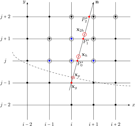
Figure 1. Spatially two-dimensional Cartesian mesh. $\bullet$ is interior point, $\filledsquare$ is ghost point, $\boxdot$ is the point at the boundary, $\largecircle$ is the point for extrapolation, the dashed line is the boundary.

For this, we first construct an interpolation stencil $\mathcal{E}$, composed of grid points of $D$. For instance, in Figure 1, the inward normal $\mathbf{n}$ intersects the grid lines $y=y_{j}$, $y_{j+1}$, $y_{j+2}$ at points $P^{*}_{0}$, $P^{*}_{1}$, $P^{*}_{2}$. Then we choose the three nearest points of the cross point $P^{*}_{l},\,l=0,1,2$, in each line, i.e. marked by a large circle. From these nine points, we can build a Lagrange polynomial $q_{2}(\mathbf{x})\in\mathbb{Q}_{2}(\mathbb{R}^{2})$. Therefore, we evaluate the polynomial $q_{2}(\mathbf{x})$ at $\mathbf{x}_{h}$ and $\mathbf{x}_{2h}$, i. e.

$$\left\{\begin{array}[]{l}\displaystyle{\phi}(\mathbf{x}_{h})\,=\,\sum_{\ell=0}^{8}w_{h,\ell}\,{\phi}(\mathbf{x}_{\ell}),\\ \\ \displaystyle{\phi}(\mathbf{x}_{2h})\,=\,\sum_{\ell=0}^{8}w_{2h,\ell}\,{\phi}(\mathbf{x}_{\ell}),\end{array}\right.$$

with $\mathbf{x}_{\ell}\in\mathcal{E}$. We thus have that $\phi_{i,j-1}$ is approximated from the interior domain.

However, in some cases, we can not find a stencil of nine interior points. For instance, when the interior domain has small acute angle sharp, the normal $\mathbf{n}$ can not have three cross points $P^{*}_{l},\,l=0,1,2$ in interior domain, or we can not have three nearest points of the cross point $P^{*}_{l},\,l=0,1,2$, in each line. In this case, we alternatively use a first degree polynomial $q_{1}(\mathbf{x})$ with a four points stencil or even a zero degree polynomial $q_{0}(\mathbf{x})$ with an one point stencil. We can similarly construct the four points stencil or the one point stencil as above.

5. Numerical simulations

5.1. One single particle motion in $3D$

Before simulating at the statistical level, we investigate on the motion of individual particles in a given magnetic field the accuracy and stability properties with respect to $\varepsilon>0$ of the semi-implicit algorithms presented in Section 3.

Numerical experiments of the present subsection are run with an electric field ${\mathbf{E}}=-\nabla_{\mathbf{x}}\phi$, with

$$\phi\,:\quad{\mathbb{R}}^{3}\to{\mathbb{R}}\,,\qquad\mathbf{x}=(x,y,z)\,\mapsto\,20\,\sqrt{x^{2}+y^{2}}+0.5\,\cos(2\pi\,z)$$

and a time-independent external magnetic field corresponding to

$$b\,:\quad{\mathbb{R}}^{3}\to{\mathbb{R}}\,,\qquad\mathbf{x}_{\perp}=(x,y,0)\,\mapsto\,\frac{1}{10^{2}\,-\,(x^{2}+y^{2})}$$

Moreover we choose for all simulations the initial data as $\mathbf{x}^{0}=(5,0,0)$, $\mathbf{v}^{0}=(4,3,2)$, whereas the final time is $T=10$. In this case, the asymptotic drift velocity predicted by the limiting model (2.15) is explicitly given by ${\mathbf{U}}^{\rm gc}$.

First, for comparison, we compute a reference solution $(\mathbf{x}^{\varepsilon},\mathbf{v}^{\varepsilon},e_{\perp}^{\varepsilon})_{\varepsilon>0}$ to the initial problem (2.4) thanks to an explicit fourth-order Runge-Kutta scheme used with a very small time step of the order of $\varepsilon$ and a reference solution $(\mathbf{x},e_{\perp},v_{\mkern 3.0mu\vphantom{\perp}\vrule depth=0.0pt\mkern 2.0mu\vrule depth=0.0pt\mkern 3.0mu})$ to the (non stiff) asymptotic model (2.15) obtained when $\varepsilon\ll 1$. Recall that the derivation of (2.15) also shows that $\mathbf{v}^{\varepsilon}$ is second order consistent to ${\mathbf{U}}^{\rm gc}\equiv{\mathbf{U}}^{\rm gc}(\mathbf{x},e_{\perp},v_{\mkern 3.0mu\vphantom{\perp}\vrule depth=0.0pt\mkern 2.0mu\vrule depth=0.0pt\mkern 3.0mu})$ when $\varepsilon\ll 1$. Then we compute an approximate solution $(\mathbf{x}^{\varepsilon}_{\Delta t},\mathbf{v}^{\varepsilon}_{\Delta t},e^{\varepsilon}_{\perp\Delta t})$ using either (3.6)–(3.9) or (3.13)-(3.19), and compare them to the reference solutions.

In Figures 2 and 3, we present trajectory on space variables between the reference solution for the initial problem (2.4) and the one obtained with the third-order scheme (3.13)-(3.19). As expected for a fixed time step $\Delta t=0.1$, the scheme is quite stable even in the limit $\varepsilon\ll 1$ and the error on the space variable is uniformly small. In contrast, for a fixed time step, the error on the velocity variable is small for large values of $\varepsilon$, but gets very large when $\varepsilon\ll 1$ since the scheme cannot follow high-frequency time oscillations of order $\varepsilon^{-1}$ when $\varepsilon\ll\Delta t$ (not presented).

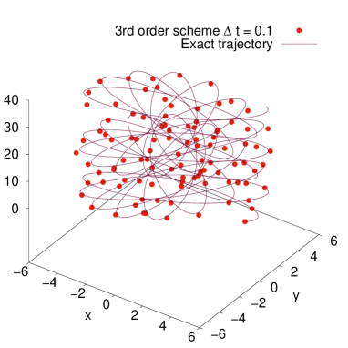
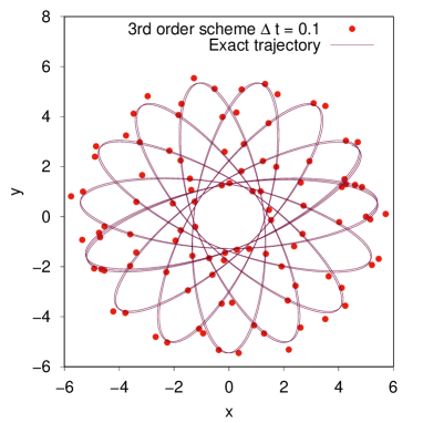
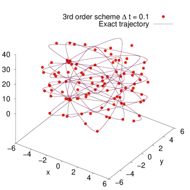
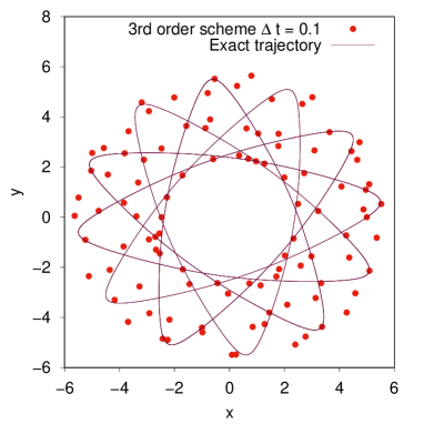
(a) $3D$	(b) $2D$

Figure 2. One single particle motion without electric field. Space trajectory (a) in three dimension, (b) $x-y$ two dimensional projection obtained with fixed time steps $\Delta t=0.1$ with third-order scheme (3.13)-(3.19), plotted as functions from top to bottom as $\varepsilon=10^{-1}$ and $10^{-2}$.

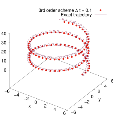
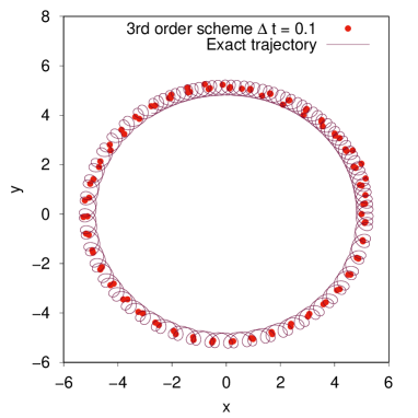
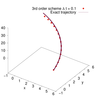
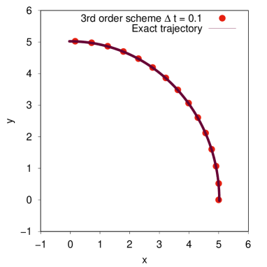
(a) $3D$	(b) $2D$

Figure 3. One single particle motion without electric field. Space trajectory (a) in three dimension, (b) $x-y$ two dimensional projection obtained with fixed time steps $\Delta t=0.1$ with third-order scheme (3.13)-(3.19), plotted as functions from top to bottom as $\varepsilon=10^{-3}$ and $10^{-4}$.

5.2. The Vlasov-Poisson system

We now consider the Vlasov-Poisson system (2.1), then ignoring the contribution of boundary conditions or assuming that the density is concentred far from the boundary, the total energy $\mathcal{E}(t)$ is given by

$$\mathcal{E}(t)\,:=\,\iint_{\Omega\times{\mathbb{R}}^{3}}f^{\varepsilon}(t,\mathbf{x},\mathbf{v})\,\frac{\|\mathbf{v}\|^{2}}{2}\,\textrm{d}\mathbf{x}\,\textrm{d}\mathbf{v}\,+\,\frac{1}{2}\int_{\Omega}\|{\mathbf{E}}^{\varepsilon}(t,\mathbf{x})\|^{2}\textrm{d}\mathbf{x}$$

and is conserved with time. Observe for the asymptotic model (2.16), the same energy can be defined as

$$\mathcal{E}(t)\,:=\,\iint_{\Omega\times{\mathbb{R}}^{3}}F^{\varepsilon}(t,\mathbf{x},e_{\perp},v_{\mkern 3.0mu\vphantom{\perp}\vrule depth=0.0pt\mkern 2.0mu\vrule depth=0.0pt\mkern 3.0mu})\,\left(e_{\perp}+\frac{|v_{\mkern 3.0mu\vphantom{\perp}\vrule depth=0.0pt\mkern 2.0mu\vrule depth=0.0pt\mkern 3.0mu}|^{2}}{2}\right)\,\textrm{d}\mathbf{x}\textrm{d}e_{\perp}\textrm{d}v_{\mkern 3.0mu\vphantom{\perp}\vrule depth=0.0pt\mkern 2.0mu\vrule depth=0.0pt\mkern 3.0mu}\,+\,\frac{1}{2}\int_{\Omega}\|{\mathbf{E}}^{\varepsilon}(t,\mathbf{x})\|^{2}\textrm{d}\mathbf{x}.$$

As far as smooth solutions are concerned, the total energy is preserved by both the original $\varepsilon$-dependent model and by the asymptotic model (2.16). One goal of our experimental observations is to check that despite the fact that our scheme dissipates some parts of the velocity variable to reach the asymptotic regime corresponding to (2.16) it does respect this conservation.

Furthermore, assuming that $b$ does not depend on time, we define the adiabatic variable given by

$$\mu(t)=\int_{\Omega}\int_{{\mathbb{R}}^{3}}f^{\varepsilon}(t,\mathbf{x},\mathbf{v})\,\frac{\|\mathbf{v}_{\perp}\|^{2}}{2b(\mathbf{x}_{\perp})}\,\textrm{d}\mathbf{x}\,\textrm{d}\mathbf{v}\,.$$

In contrast to the energy, an essentially exact conservation of the adiabatic variable is a sign that we have reached the limiting asymptotic regime since it does not hold for the original model but does for the asymptotic (2.16) as $b$ is time-independent and ${\mathbf{E}}$ is curl-free. Observe that, since $b$ is not homogeneous, even in the asymptotic regime the kinetic and potential parts of the total energy are not preserved separately, but the total energy corresponding to the Vlasov-Poisson system is still preserved.

Diocotron instability in a cylinder.

Here we choose $\Omega=D\times(0,L_{z})$ with $D=D(0,6)$ the disk centered at the origin with radius $6$ and $L_{z}=1$. Our simulations start with an initial data that is Maxwellian in velocity and whose macroscopic density is the sum of two Gaussians, explicitly

$$f_{0}(\mathbf{x},\mathbf{v})\,=\,\frac{n_{0}(\mathbf{x})}{(2\pi)^{3/2}}\,\exp\left(-\frac{\|\mathbf{v}\|^{2}}{2}\right),$$

where $n_{0}$ is chosen as

$$n_{0}(\mathbf{x})=\left\{\begin{array}[]{ll}\displaystyle n_{0}\,\left(1\,+\,\alpha(\cos(\theta)+5\,\cos(2\pi\,k_{z}\,z))\right)&{\rm\,if\,}6\leq r_{\perp}\leq 7,\\ \\ \displaystyle 0&{\rm\,else,}\end{array}\right.$$

with $r_{\perp}=\|\mathbf{x}_{\perp}\|$, $\theta=\arctan(y/x)$, $n_{0}=4000$, $k_{z}=3$ and $\alpha=0.001$. Moreover, in the Poisson equation (2.2) we take $\rho_{0}=0$. The parameter $\varepsilon$ is chosen as $\varepsilon=0.05$, where the asymptotic regime is relevant. We compute numerical solutions to the Vlasov-Poisson system (2.1) with the third-order scheme (3.13)-(3.19) and time step $\Delta t=0.1$. We first run one set of numerical simulations homogeneous magnetic field $b=1$.

In Figure 4 we present the time evolution of the relative variation of energy and adiabatic variable. For instance,

$$\Delta\mathcal{E}_{\alpha}=\frac{\mathcal{E}_{\alpha}(t)-\mathcal{E}_{\alpha}(0)}{\mathcal{E}_{\alpha}(0)},\quad\alpha\in\{k,p,t\},$$

where $k$ denotes the kinetic energy, $p$ is the potential energy and $t$ is the total energy. Notice that total energy is conserved at the continuous level but not with our numerical scheme. However, we show that all these features are captured satisfactorily by our scheme even on long time evolutions with a large time step and despite its dissipative implicit nature in the asymptotic regime when $\varepsilon=0.05$.

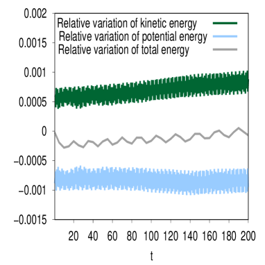
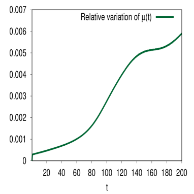
(a) $\Delta\mathcal{E}(t)$	(b) $\Delta\mu(t)$

Figure 4. Diocotron instability in a cylinder. Time evolution of total energy and adiabatic invariant with $\varepsilon=0.05$ obtained using (3.13)-(3.19) with $\Delta t=0.5$.

In Figure 5 we visualize the corresponding dynamics by presenting some snapshots of the time evolution of the macroscopic charge density. We take $\varepsilon=0.05$ such that the magnetic field is sufficiently large to provide a good confinement of the macroscopic density. Here, we expect similar results as for the two dimensional diocotron instability where seven vortices are generated [13, 14].

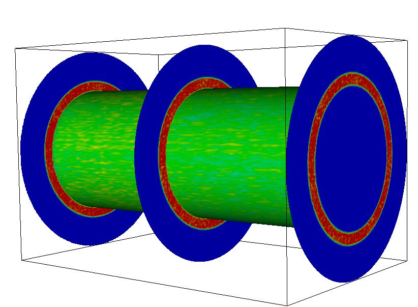
$t=000$	$t=040$
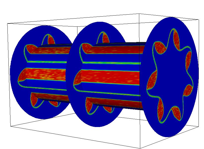
$t=080$	$t=120$
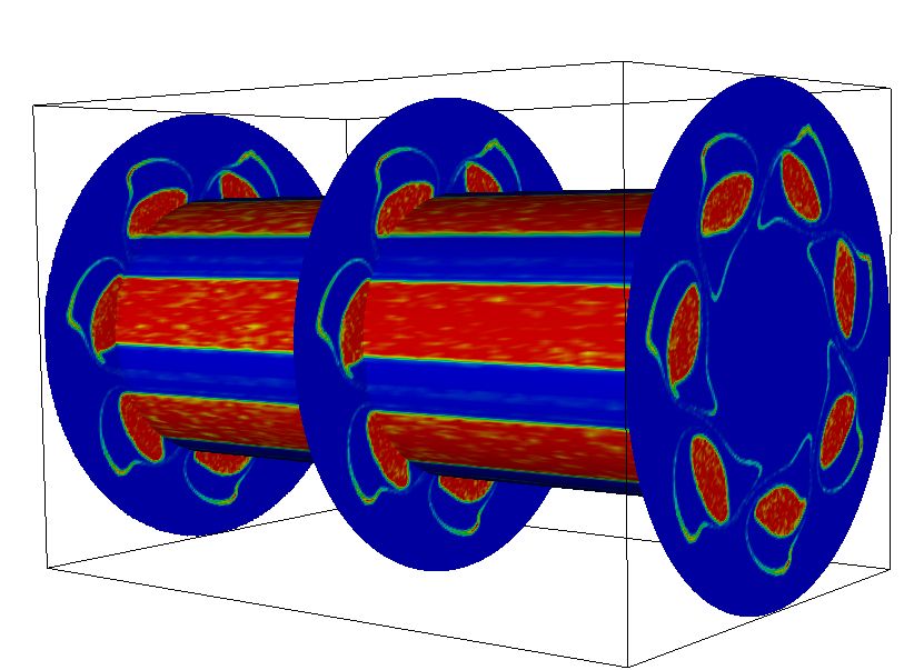
$t=140$	$t=200$

Figure 5. Diocotron instability in a cylinder. Snapshots of the time evolution of the macroscopic charge density $\rho$ when $\varepsilon=0.05$, obtained using (3.13)-(3.19) with $\Delta t=0.5$ .

Fusion of vertices in a $D$-shaped domain

We consider now a D-shaped domain in the plane orthogonal to the magnetic field $D$ presented in Section IV of [23] and depicted in Figure 6 (a). The mapping from curvilinear coordinates $\mathbf{\xi}=(\xi_{1},\xi_{2})$ to physical coordinates $\mathbf{x}_{\perp}=(x,y)$ is given by

$$\left\{\begin{array}[]{l}x\,=\,x_{c}+\xi_{1}\,\cos\left(\xi_{2}\,+\,\arcsin(0.416)\sin(\xi_{2})\right),\\[8.53581pt] y\,=\,y_{c}\,+\,1.66\,\xi_{1}\,\sin(2\pi\xi_{2}),\end{array}\right.$$

for $0\leq\xi_{1}\leq R_{0}$ and $0\leq\xi_{2}\leq 2\pi$ with $(x_{c},y_{c})=(0,0)$ and $R_{0}=10$.

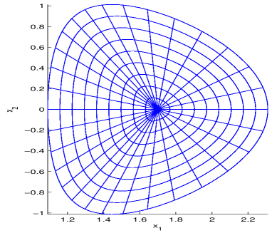
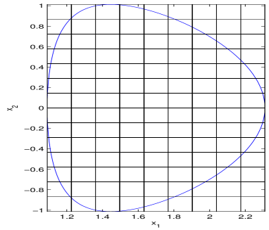
(a)	(b)

Figure 6. D-shaped domain [23]. (a) Constant lines in coordinates $\xi=(\xi_{1},\xi_{2})$; (b) D-shaped domain embedded in Cartesian mesh.

Our simulations start with an initial data that is Maxwellian in velocity and whose macroscopic density is the sum of two Gaussians in the perpendicular plane to the magnetic field and a perturbed constant homogeneous density in the parallel direction to the magnetic field, explicitly

$$f_{0}(\mathbf{x},\mathbf{v})\,=\,\frac{n_{0}(z)}{8\pi^{2}r_{0}^{2}}\left[\exp\left(-\frac{\|\mathbf{x}_{\perp}-\mathbf{x}_{0\perp}\|^{2}}{2r_{0}^{2}}\right)+\exp\left(-\frac{\|\mathbf{x}_{\perp}+\mathbf{x}_{0\perp}\|^{2}}{2\,r_{0}^{2}}\right)\right]\,\exp\left(-\frac{\|\mathbf{v}\|^{2}}{2}\right),$$

with $\mathbf{x}_{0\perp}=(3/2,-3/2,0)$, $r_{0}=3$ and the density $n_{0}(z)=5000\,(1+\alpha\cos(k_{z}\,z))$ with $k_{z}=2\pi/L_{z}$.

We choose a time-independent inhomogeneous magnetic field

$$b\,:\quad{\mathbb{R}}^{2}\to{\mathbb{R}}\,,\qquad\mathbf{x}\,\mapsto\,\frac{20}{\sqrt{20^{2}-\|\mathbf{x}_{\perp}\|^{2}}},$$

that is, radial increasing with value one at the origin.

In Figure 7 we present again the time evolution of the relative variation of energy and adiabatic variable. In this regime, the limit model (2.16) makes sense and it is expected that both the total energy $\mathcal{E}$ and the adiabatic invariant $\mu$ are conserved. Once again the numerical results are satisfactory since even for large times, the relative variations are of order $10^{-3}$.

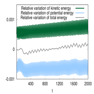
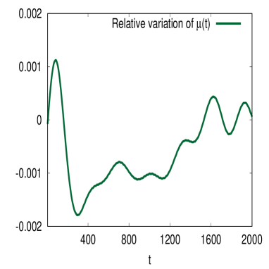
(a) $\Delta\mathcal{E}_{\alpha}(t)=\frac{\mathcal{E}_{\alpha}(t)-\mathcal{E}_{\alpha}(0)}{\mathcal{E}_{\alpha}}$	(b) $\Delta\mu(t)=\frac{\mu(t)-\mu(0)}{\mu(0)}$

Figure 7. Fusion of vertices in a $D$-shaped domain. Time evolution of (a) total energy, kinetic energy and potential energy (b) adiabatic invariant with $\varepsilon=0.01$ obtained using (3.13)-(3.19) with $\Delta t=0.5$.

In Figure 8 we visualize the corresponding dynamics by presenting some snapshots of the time evolution of the macroscopic charge density. We take $\varepsilon=0.01$ such that the magnetic field is sufficiently large to provide a good confinement of the macroscopic density. At time $t=30$, some filament structures can be identified. These filaments are observed more clearly for larger times. Since the intensity of the magnetic field is sufficiently large, the plasma is well confined and the two vertices merge, whereas some the filaments persist and generate a “halo” which propagates in the domain.

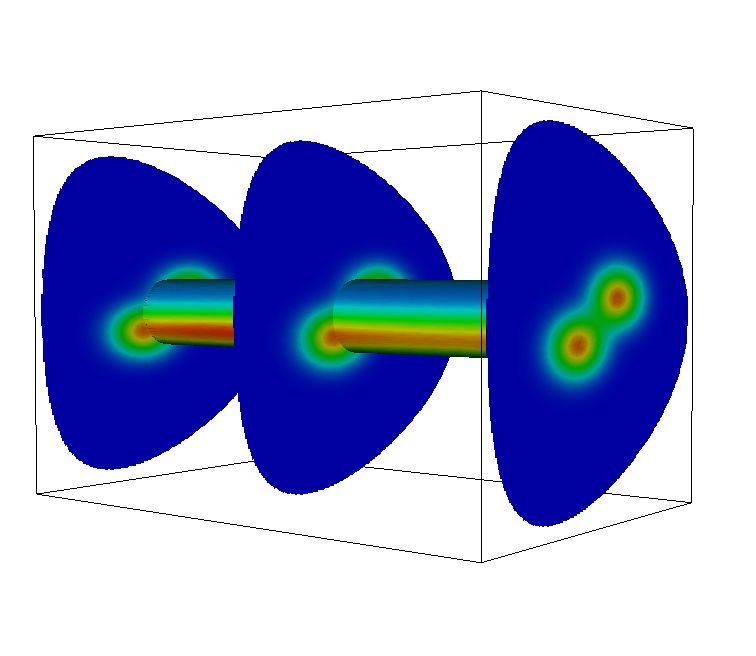
$t=0000$	$t=0160$
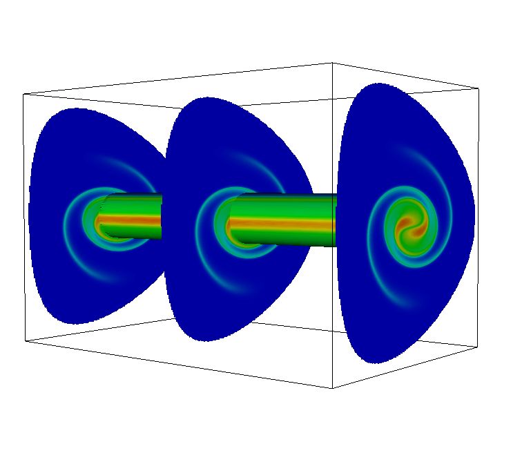
$t=0480$	$t=0640$
$t=0960$	$t=1920$

Figure 8. Fusion of vertices in a $D$-shaped domain. Snapshots of the time evolution of the macroscopic charge density $\rho$ when $\varepsilon=0.01$, obtained using (3.13)-(3.19) with $\Delta t=0.5$ .

6. Conclusion and perspective

In the present paper we have proposed a class of semi-implicit time discretization techniques for particle-in cell simulations of the three dimensional Vlasov-Poisson system. The main feature of our approach is to guarantee the accuracy and stability on slow scale variables even when the amplitude of the magnetic field becomes large including cases with non homogeneous magnetic fields and coarse time grids. Even on large time simulations the obtained numerical schemes also provide an acceptable accuracy on physical invariants (total energy for any $\varepsilon$, adiabatic invariant when $\varepsilon\ll 1$) whereas fast scales are automatically filtered when the time step is large compared to $\varepsilon$.

As a theoretical validation we have proved that the discrete trajectories remain bounded for the semi-implicit schemes and for $\varepsilon\ll 1$, the schemes is consistent with the asymptotic model and preserve the order of accuracy with respect to $\Delta t$. From a practical point of view, the next natural step would be to consider the genuinely three-dimensional Vlasov-Poisson system taking into account curvature effects.

7. Acknowledgements

Francis Filbet was supported by the EUROfusion Consortium and has received funding from the Euratom research and training programme 2014-2018 under grant agreement No. 633053. The views and opinions expressed herein do not necessarily reflect those of the European Commission.

Chang Yang was supported by National Natural Science Foundation of China (Grant No. 11401138).

References

- [1] C. K. Birdsall, A. B. Langdon, Plasma Physics via Computer Simulation Institute of Physics Publishing, Bristol and Philadelphia., (1991).
- [2] S. Boscarino, F. Filbet and G. Russo, High order semi-Implicit schemes for time dependent partial differential equations, J. Scientific Computing, (2016).
- [3] M. Bostan, Asymptotic behavior for the Vlasov-Poisson equations with strong external magnetic field. Straight magnetic field lines preprint (2018).
- [4] M. Bostan and A. Finot, The finite Larmor radius regime for the Vlasov-Poisson equations. The three dimensional setting with non uniform magnetic field preprint (2018).
- [5] G.-H. Cottet and P. Koumoutsakos, Vortex Methods: Theory and Practice. Cambridge University Press, Cambridge, (2000).
- [6] N. Crouseilles, M. Lemou and F. Méhats, Asymptotic preserving schemes for highly oscillatory Vlasov–Poisson equations, Journal of Computational Physics, 248, pp. 287–308 (2013).
- [7] N. Crouseilles, E. Frénod, S. Hirstoaga, A. Mouton, Two-Scale Macro-Micro decomposition of the Vlasov equation with a strong magnetic field, Math. Models Methods Appl. Sci. 23, (2015).
- [8] N. Crouseilles, M. Lemou, F. Méhats, X. Zhao, Uniformly accurate forward semi-Lagrangian methods for highly oscillatory Vlasov-Poisson equations, SIAM Multiscale Model. Simul. (2017).
- [9] N. Crouseilles, M. Lemou, F. Mehats, X. Zhao, Uniformly accurate Particle-in-Cell method for the long time two-dimensional Vlasov-Poisson equation with strong magnetic field, (2017).
- [10] N. Crouseilles, S. Hirstoaga, X. Zhao, Multiscale Particle-in-Cell methods and comparisons for the long time two-dimensional Vlasov-Poisson equation with strong magnetic field, Comput. Phys. Comm. 222, pp. 136-151, (2018).
- [11] P. Degond and F. Deluzet, Asymptotic-preserving methods and multiscale models for plasma physics. J. Comput. Phys. 336 (2017), pp. 429–457.
- [12] P. Degond and F. Filbet, On the asymptotic limit of the three dimensional Vlasov-Poisson system for large magnetic field: formal derivation. J. Stat. Phys. 165 (2016), no. 4, 765–784.
- [13] F. Filbet and L. M. Rodrigues, Asymptotically stable particle-in-cell methods for the Vlasov-Poisson system with a strong external magnetic field, SIAM J. Numer. Anal., 54 (2), pp 1120–1146, (2016).
- [14] F. Filbet and L. M. Rodrigues, Asymptotically Preserving Particle-in-Cell Methods for Inhomogeneous Strongly Magnetized Plasmas, SIAM J. Numer. Anal., 55(5), pp 2416–2443, (2017).
- [15] F. Filbet and E. Sonnendrücker, Comparison of Eulerian Vlasov solvers, Computer Physics Communications, 150, pp. 247–266 (2003).
- [16] E. Frénod, S. Hirstoaga, M. Lutz and E. Sonnendrücker, Long Time Behaviour of an Exponential Integrator for a Vlasov-Poisson System with Strong Magnetic Field. Commun. Comput. Phys. 18, no. 2, 263–296 (2015).
- [17] E. Frénod, E. Sonnendrücker, Long time behavior of the Vlasov equation with strong external magnetic field, Math. Models Methods Appl. Sci. 19, 539-553, (2000).
- [18] V. Grandgirard, M. Brunetti, P. Bertrand, N. Besse, X. Garbet, P. Ghendrih, G. Manfredi, Y. Sarazin, O. Sauter, E. Sonnendrücker, J. Vaclavik, L. Villard, A drift-kinetic Semi-Lagrangian 4D code for ion turbulence simulation, Journal of Computational Physics, 217 (2006), 395–423.
- [19] R.D. Hazeline and A.A. Ware, The drift kinetic equation for toroidal plasmas with large mass velocities. Plasma Phys., 20, pp. 673–678 (1978).
- [20] R.D. Hazeline and J.D. Meiss, Plasma Confinement. Dover Publications, Mineola. (2003).
- [21] H. Johansen and P. Colella, A Cartesian Grid Embedded Boundary Method for Poisson’s Equation on Irregular Domains, Journal of computational physics, 147 (1998), pp. 60–85.
- [22] P. Koumoutsakos, Inviscid Axisymmetrization of an Elliptical Vortex. Journal of Computational Physics 138, 821–857 (1997).
- [23] R.L. Miller, M.S. Chu, J.M. Greene, Y.R. Lin-Liu, R.E. Waltz, Noncircular, finite aspect ratio, local equilibrium model, Physical Plasmas, 5(4) (1998), pp. 973–978.
- [24] R. Kleiber, R. Hatzky, A. Konies, A. Mishchenko and E. Sonnendrücker, An explicit large time step particle-in-cell scheme for nonlinear gyrokinetic simulations in the electromagnetic regime. Physics of Plasmas 23, 032501 (2016)
- [25] M. Kraus, K. Kormann, P. Morrison and E. Sonnendrücker, GEMPIC: geometric electromagnetic particle-in-cell methods. Journal of Plasma Physics 83 (4), 905830401 (2017)
- [26] H. Qin et al, Canonical symplectic particle-in-cell method for long-term large-scale simulations of the Vlasov-Maxwell system Nucl. Fusion, 56, 014001 (2016).
- [27] L. Saint-Raymond, Control of large velocities in the two-dimensional gyro-kinetic approximation. J. Math. Pures Appl. 81, no. 4, 379–399 (2002).
- [28] T. Utsumi , T. Kunugi, J. Koga, A numerical method for solving the one-dimensional Vlasov-Poisson equation in phase space, Computer Physics Communications, 108 (1998), pp. 159–179.
- [29] J. Xiao, H. Qin, J. Liu, Y. He, R. Zhang, and Y. Sun, Explicit high-order non-canonical symplectic particle-in-cell algorithms for Vlasov-Maxwell systems, Physics of Plasmas , 22, 112504 (2015).