Non-Gaussianity of van Hove Function and Dynamic Heterogeneity Length Scale

Abstract

Non-Gaussian nature of the probability distribution of particles’ displacements in the supercooled temperature regime in glass-forming liquids are believed to be one of the major hallmarks of glass transition. It is already been established that this probability distribution which is also known as the van Hove function show universal exponential tail. The origin of such an exponential tail in the distribution function is attributed to the hopping motion of particles observed in the supercooled regime. The non-Gaussian nature can also be explained if one assumes that the system has heterogeneous dynamics in space and time. Thus exponential tail is the manifestation of dynamic heterogeneity. In this work we directly show that non-Gaussanity of the distribution of particles’ displacements occur over the dynamic heterogeneity length scale and dynamical behaviour course grained over this length scale becomes homogeneous. We study the non-Gaussianity of van Hove function by systematically coarse graining at different length scale and extract the length scale of dynamic heterogeneity at which the shape of the van Hove function crosses over from non-Gaussian to Gaussian. The obtained dynamic heterogeneity scale is found to be in very good agreement with the scale obtained from other conventional methods.

I Introduction

The distribution of displacement of particles, also known as van Hove function Van Hove (1954) shows non-Gaussian behaviour in the supercooled temperature (density) regime as demonstrated in Fig.1 for the well studied Kob-Andersen model of glass forming liquids. This has already been established as one of the main manifestations of dynamic heterogeneity in the dynamics of supercooled glass-forming liquids. Non-Gaussianity is also observed in many out of equilibrium systems that show glass like dynamical behaviour e.g., vibrated granular medium. It has been observed that the non-Gaussianity in the van Hove function appears generically as an exponential tail Chaudhuri et al. (2007). A continuous time random walk (CTRW) approach to such an observation, suggests that one can understand the appearance of such an exponential tail in the van Hove distribution, if one assumes that the particles in the systems are performing jump like (hopping) motion between two successive localized diffusive motions. The range of the exponential tail depends on the the diffusivity of the local motion and the waiting time distribution for the successive hopping motions. By carefully choosing the parameters one can fit the observed non-Gaussian feature of the van Hove function in a wide variety of systemsChaudhuri et al. (2007).

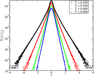
Figure 1: van Hove function for 3dKA model for different temperatures. The non Gaussian tail becomes very prominent with decreasing temperature. The line passing through the data points are the one obtained using Eq.9 (see text for details).

A different approach to rationalize the observed non-Gaussian behaviour in van Hove function is to assume spatial heterogeneity in the diffusion constants of constituent particles. Historically this idea has been introduced to understand the break down of Stokes-Einstein relation in supercooled liquids. In liquids, the Stokes-Einstein (SE) relation Hansen and McDonald ; Einstein (1905); Landau and Lifshitz relates the shear viscosity ($\eta$) to the translational diffusion constant ($D$) of a particle as $D=\frac{AT}{\eta}$, where $A$ is a constant. The value of this constant depends on the details of the particle and boundary conditions and $T$ is the temperature. This relation is derived for a probe particle in the hydrodynamic limit, but the SE relation is found to hold for the self diffusion of liquid particles also at high temperatures Hodgdon and Stillinger (1993). In the supercooled temperature regime the relation is found to break down Pollack (1981); Rössler (1990); Fujara et al. (1992); Kob and Andersen (1994); Tarjus and Kivelson (1995); Chang and Sillescu (1997); Ediger (2000); Monaco et al. (2001); Michele and Leporini (2001); Swallen et al. (2003); Chen et al. (2006); Becker et al. (2006); Xu et al. (2009); Berthier and Biroli (2011); Mallamace et al. (2010). Initially Stillinger and Hodgdon Hodgdon and Stillinger (1993) and later Tarjus and Kivelson Tarjus and Kivelson (1995) phenomenologically proposed that by considering supercooled liquids to consist of mobile “fluid-like” and less mobile “solid-like” regions, the break down of the Stokes-Einstein relation can be explained naturally as the average diffusion constant is predominantly determined by the “fluid like” regions whereas the average relaxation time is dominated by the “solid-like” regions. The clusters consisting of “fluid-like” or “solid-like” particles has been detected in many different studies Kegel et al. (2000); Weeks et al. (2000); Widmer-Cooper et al. (2008); Bhowmik et al. (2016).

For an example, if one considers a system with regions that have two diffusivities - one for “solid like” ($D_{s}$ ) and the other for “liquid like” regions ($D_{l}$). The the distribution of diffusivity can be written as $p(D)=A\delta(D_{s})+B\delta(D_{l})$ where $A$ and $B$ are fixed by the normalization condition and the amount of solid like and liquid like regions. The van Hove function will then read as

$$G_{s}(x,t)=\int dDp(D)g(x|D),$$ (1)

where $g(x|D)=\frac{1}{\sqrt{4\pi Dt}}\exp{\left(-\frac{x^{2}}{4Dt}\right)}$ is the distribution of displacement of particles undergoing diffusive process. With Eq.1 it can be shown that the van Hove function will have a long tail and depending on the distribution of the $p(D)$, the tail of the distribution can be either exponential or even Gaussian Wang et al. (2012). In general the exponential tail has been reported Chaudhuri et al. (2007) which, as emphasized in Wang et al. (2012), might be due to the small range of the data.

A natural question that arises in this context is as follows. If one measures dynamical quantities like van Hove function using coarse-grained over certain length scale, will the dynamics looks spatially homogeneous? For example, if we calculate van Hove function coarse-grained over some specific length scale, will it loose its non Gaussian tail and will become Gaussian. If the answer is affirmative, then this will give us a natural procedure to extract the underlying dynamic heterogeneity length scale. This will also directly prove the picture of supercooled liquid being mosaic structure of fluid-like and solid-like regions with size of these structures being equal to the dynamic heterogeneity length scale. In Ref.Parmar et al. (2017), it is shown that if one calculates the wave-vector dependent $\alpha$-relaxation time, $\tau_{\alpha}(q)$ in the supercooled temperature regime, then one finds that Stokes-Einstein relation does not break down above a characteristic wave vector, $q^{*}$ which depends on the studied temperature, $T$. The inverse of this characteristic wave vector defines a length scale, $\xi^{*}(T)=2\pi/q^{*}(T)$. This length scale, $\xi^{*}(T)$ is found to be same as that of the dynamic heterogeneity length scale obtained from the analysis of four-point dynamic susceptibility Dasgupta et al. (1991), $\chi_{4}(T,t)$ calculated at $\alpha$-relaxation time, $t=\tau_{\alpha}(q=q_{0})$. $q_{0}$ is the position of the first peak in the static structure factor, $S(q)$. This study also suggests that dynamics coarse-grained over dynamic heterogeneity length scale might look homogeneous, leading to a direct measure of dynamic heterogeneity length scale from experimental data.

The goal of the present work is to measure the non-Gaussian behaviour of van Hove function by systematically coarse graining the dynamics over different length scale to study the cross over from non-Gaussian to Gaussian form at some characteristic length scale. Then understand the relation between this characteristic length scale with the dynamic heterogeneity length scale obtained from the conventional methods. For systematic coarse-graining, we have employed the block analysis Chakrabarty et al. (2017) which has recently been used very successfully to perform finite size scaling analysis of four-point susceptibility, $\chi_{4}(t)$.

The rest of the paper is organized as follows. First we will discuss the model glass-forming systems that are studied in this work and the details of the simulation performed. Then we will discuss the correlation functions and the method of block analysis that has been employed to do the systematic coarse-graining of the dynamics. Next we will discuss how distribution of diffusion constants are extracted from the van Hove function using iterative methods. Finally, we will discuss the results and conclude with possible application of this results for experimentally relevant systems.

II Models and Simulation Details

We have studied three different model glass forming liquids in three dimensions for $N=108000$. The model details are given below: 3dKA: The model glass former, we have studied is the Kob-Anderson $80:20$ Kob and Andersen (1995) Lenard-Jones Binary mixture. This model was first introduced by Kob-Anderson to simulate $Ni_{80}P{20}$. This model has been studied extensively by many people and found to be a very good glass former in three dimensions. The interaction potential is given by

$$V_{\alpha\beta}(r)=4.0\epsilon_{\alpha\beta}[(\frac{\sigma_{\alpha\beta}}{r})^{12}-(\frac{\sigma_{\alpha\beta}}{r})^{6}]$$

where $\alpha,\beta\in\{A,B\}$ and $\epsilon_{AA}=1.0$, $\epsilon_{AB}=1.5$, $\epsilon_{BB}=0.5$; $\sigma_{AA}=1.0$, $\sigma_{AB}=0.80$, $\sigma_{BB}=0.88$. The interaction potential is cut off at $2.50\sigma_{\alpha\beta}$ and the number density is $\rho=1.20$. Length, energy and time scale are measured in units of $\sigma_{AA},\epsilon_{AA}$ and $\sqrt{\frac{\sigma_{AA}^{2}}{\epsilon_{AA}}}$. For Argon these units corresponds to a length of $3.4\AA$, an energy of $120Kk_{\beta}$ and time of $3\times 10^{-13}s$. We have done simulation in the temperature range $T\in\{0.430,0.800\}$.

3dIPL: In this model, the inter particle interaction potential is modeled as purely repulsive inverse Power Law form. This model has been studied in Pedersen et al. (2010). We have studied in the temperature range $T\in\{0.450,0.800\}$ The interaction potential is given by

$$V_{\alpha\beta}(r)=1.945\epsilon_{\alpha\beta}[(\frac{\sigma_{\alpha\beta}}{r})^{15.48}]$$

All the parameters and interaction cut-off is same as the 3dKA model.

3dR10: This is a 50:50 binary mixture Karmakar et al. (2010) interacting via the pair wise interaction potential

$$V_{\alpha\beta}(r)=\epsilon_{\alpha\beta}[(\frac{\sigma_{\alpha\beta}}{r})^{10}]$$

Here $\epsilon_{\alpha\beta}=1.0$, $\sigma_{AA}=1.0$, $\sigma_{AB}=1.22$, $\sigma_{BB}=1.40$. The interaction potential is cut-off at $1.38\sigma_{\alpha\beta}$. The number density of particle is 0.85 and the temperature range studied is $T\in\{0.520,0.800\}$.

We use the modified leap-frog algorithm with the Berendsen thermostat to keep the temperature constant in the simulation runs. Any other thermostat does not change the results qualitatively as we are mostly interested in configurational changes in the system instead of momentum correlations. The integration time steps used is $dt=0.005$ in the studied temperature range.

To characterize the dynamics, we have calculated two point correlation function $Q(t)$, which gives the amount of overlap between two configurations which are separated by time $t$.

$$Q(t)=\sum_{i=1}^{N}w(\left|r_{i}(0)-r_{i}(t)\right|),$$ (2)

where the window function $w(x)=1$ when $x\leq a$ and $0$ otherwise. We choose $a=0.3$ which is close to the plateau value of the mean square displacement. This parameter is chosen to remove possible decorrelation that can happen due to vibrational motion of the particles inside the cage formed by their neighbours. A different choice of this parameter does not change the temperature dependence of the $\alpha$-relaxation time, $\tau_{\alpha}$. $\tau_{\alpha}$ is defined from the decay of $Q(t)$ as $\langle Q(\tau_{\alpha})\rangle=1/e$. $\langle\ldots\rangle$ refers to ensemble average and averaging over different time origin. The fluctuation or variance of the overlap function $Q(t)$ is defined as four point susceptibility Dasgupta et al. (1991).

$$\chi_{4}^{p}(t)=\frac{1}{N}[\langle Q^{2}(t)\rangle]-\langle Q(t)\rangle^{2}]$$

Dynamic length-scale, $\xi_{D}$ can be obtained from the finite size scaling of peak height of $\chi_{4}(t)$ very reliably Karmakar et al. (2009). In this study, we have taken the results of $\xi_{D}$ from Ref.Chakrabarty et al. (2017). It is important to note that peak of $\chi_{4}(t)$ appears at $t=\tau_{4}$, which is very close to $\tau_{\alpha}$. This also suggests that heterogeneity is maximum at time scale close to the $\alpha$-relaxation time. In this study thus we will look at the van Hove function at the same time scale.

III Results

We start with the formal definition of the van Hove correlation function

$$G_{s}(x,\tau)=\left<\delta\left[x-(x_{i}(\tau)-x_{i}(0))\right]\right>,$$ (3)

where the $\langle\ldots\rangle$ implies the averaging over the time origin and different statistically independent samples.

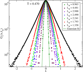
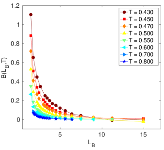
Figure 2: Top Panel: van Hove correlation function as a function of displacement for different coarse-graining block length, $L_{B}$. These data are for 3dKA model. One can clearly see that as one increases the block length, the nature of the distribution changes to Gaussian. All the curves are shifted to match the peak height. The line passing through the data for $L_{B}=8.963$ is a Gaussian fit to the data. Bottom Panel: The Binder cumulant as a function of block length for different temperature. Binder cumulant becomes 0 for Gaussian distribution. Thus one can clearly see that for smaller block length the distribution is very non Gaussian and becomes Gaussian at larger block length. The cross over length increases with decreasing temperature.

To perform systematic spatial coarse-graining of the dynamics, we have used the method of block analysis Avila et al. (2014); Chakrabarty et al. (2017). In this method, the whole simulation box is divided into smaller blocks of length, $L_{B}$. Thus with block size of $L_{B}$, there will be $N_{B}=(L/L_{B})^{d}$, number of blocks in the system. $L$ is the linear size of the simulation box and $d$ is the number of spatial dimensions. This method is shown to be very attractive for doing finite size scaling of four-point susceptibility $\chi_{4}(t)$ for extracting dynamic heterogeneity length scale, $\xi_{D}$. Due to its simplicity, the method will be very useful to study dynamic heterogeneity in experiments with colloidal particles. In this work, we have defined a coarse-grained displacement as

$$\Delta x_{j}^{B}(\tau)=\sum_{i=1}^{n_{j}}\left[x_{i}(\tau)-x_{i}(0)\right],$$ (4)

where $n_{j}$ is the number of particles in the $j^{th}$ block. Note that this number will be different for different blocks. Then we define the blocked van Hove function as

$$G^{B}_{s}(x,\tau)=\left<\sum_{j=1}^{N_{B}}\delta\left[x-\Delta x_{j}^{B}(\tau)\right]\right>,$$ (5)

By varying the block length, $L_{B}$ we have studied how the non-Gaussianity changes with increasing block length. One thing to note is that, as one increases the block length the total displacement decreases, this is easy to understand as there is no center of mass displacement during the simulation and if we choose $L_{B}=L$, then the coarse-grained displacement will be zero. As we are interested in the shape of the van Hove function this issue will not affect the analysis.

In top panel Fig.2, we have shown the van Hove function for $T=0.470$ for 3dKA model for various coarse-graining block length, $L_{B}$. One can clearly see that with increasing block length, the distribution becomes more and more Gaussian and for block length $L_{B}=7.469$, at this particular temperature, the distribution becomes completely Gaussian as shown by the fitted line to a Gaussian function. In the bottom panel, we have calculated the binder cumulant of the distribution to measure the departure from the Gaussian form. The binder cumulant is defined as

$$B(L_{B},T)=1-\frac{\langle x^{4}\rangle}{3\langle x^{2}\rangle^{2}}$$ (6)

which is zero for a Gaussian distribution. The average is done over the distribution, $G_{s}^{B}(x,\tau)$ for the respective block length $L_{B}$. The bottom panel of Fig.2, shows that binder cumulant is non-zero for smaller block sizes and tends to become zero for larger block lengths. The approach to zero happens at larger block length for decreasing temperature.

Next we discuss how the underlying distribution of diffusion constants changes with coarse-graining volume. Before going in to the results, we explain briefly the method used to extract the distribution of diffusivity directly from the van Hove correlation function $G_{s}(x,\tau_{\alpha})$ using the Iterative algorithm suggested in Ref.Lucy (1974) and recently used in Wang et al. (2012) for the diffusion processes in biological systems and in Sengupta and Karmakar (2014); Bhowmik et al. (2016) for dynamics in supercooled liquids. If one assumes that particle displacements are due to diffusion processes and there is a distribution of local diffusivity $p(D)$, then formally we have

$$G_{s}(x,\tau_{\alpha})=\int_{0}^{D_{0}}p(D).g(x|D).dD,$$ (7)

where $g(x|D)=1/\sqrt{4\pi D\tau_{\alpha}}\exp\left(-x^{2}/4D\tau_{\alpha}\right)$ and $D_{0}$ is the upper limit of diffusion constant and will be equal to diffusivity for a free particle diffusion.

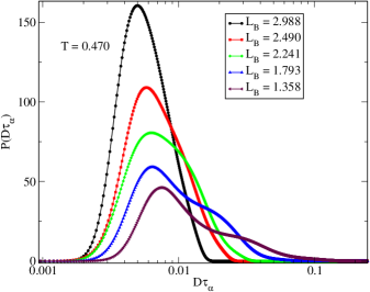
Figure 3: Distribution of diffusion constants obtained for coarse-grained van Hove function for the data in Fig.2. One can clearly see that distribution becomes bimodal to unimodal with increasing block size.

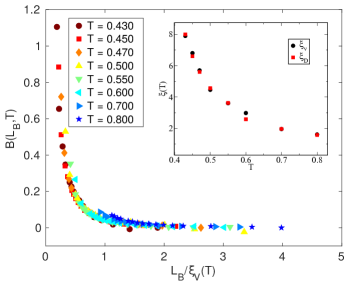
Figure 4: Top panel: Finite size scaling of binder cumulant of the van Hove functions calculated for different block lengths. The scaling collapse is quite good. This suggests the existence of a cross over length scale that grows with decreasing temperature. Inset: Comparison of the cross over length scale, $\xi$ with dynamic heterogeneity length scale, $\xi_{D}$.

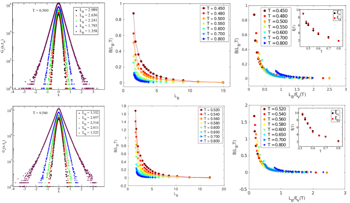
Figure 5: Top left panel: Blocked van Hove function for different block lengths for 3dIPL model. One can clearly see the shape of the van Hove function changes from non Gaussian with exponential tail to Gaussian. The curves are shifted for better clarity. Top middle panel: Binder cumulant of the blocked van Hove function for 3dIPL model again quantitatively showing the non-Gaussian to Gaussian cross over with increasing block size. Top right panel: Finite size scaling of binder cumulant of the van Hove functions. The scaling collapse is quite good. The inset shows the comparison of the cross over length scale, $\xi$ with dynamic heterogeneity length scale, $\xi_{D}$. Bottom panels: Similar analysis done for 3dR10 model.

Now given the $G_{s}(x,\tau_{\alpha})$, $p(D)$ can be calculated using Lucy’s Iterative method Lucy (1974) as

$$p^{n+1}(D)=p^{n}(D)\int_{-\infty}^{\infty}\frac{G_{s}(x,\tau_{\alpha})}{G^{n}_{s}(x,\tau_{\alpha})}g(x|D)dx,$$ (8)

where $p^{n}(D)$ is the estimate of $p(D)$ in the $n^{th}$ iteration with $p^{0}(D)=(1/D_{avg})\exp(-D/D_{avg})$ is the initial input guess distribution. Note that actual form of this guess distribution does not change the final outcome. After $n^{th}$ iteration, $G^{n}_{s}(x,\tau_{\alpha})$ can be written as

$$G^{n}_{s}(x,\tau_{\alpha})=\int_{0}^{D_{0}}p^{n}(D).g(x|D).dD.$$ (9)

Similarly

$$P^{n+1}(D\tau_{\alpha})=P^{n}(D\tau_{\alpha})\int_{-\infty}^{\infty}\frac{G_{s}(x,\tau_{\alpha})}{G^{n}_{s}(x,\tau_{\alpha})}g(x|D)dx,$$ (10)

where $p(D)dD=P(D\tau_{\alpha})d(D\tau_{\alpha})$. The choice of $D\tau_{\alpha}$ as our variable is due to the fact that $D$ changes by orders of magnitude in the studied temperature range whereas $D\tau_{\alpha}$ should change relatively modestly with decreasing temperature and it will be easier to compare the distribution obtained for different temperatures. In Fig.3, we have shown that obtained distribution of diffusion constants for the 3dKA model system at $T=0.470$. The distributions are obtained for the blocked van Hove function shown in Fig.2. These results also clearly show that the underlying distribution of diffusion constant becomes unimodal from bimodal with increasing block length.

We next perform the finite size scaling analysis of the binder cumulant to obtain the coarse-graining length scale above which the van Hove function becomes Gaussian. We assume the following form of the scaling function

$$B(L_{B},T)=\mathcal{G}[L_{B}/\xi_{V}(T)].$$ (11)

In Fig.4, we have shown the finite size scaling of the binder cumulant of the van Hove function calculated for different block sizes for the 3dKA model. The scaling collapse observed to be quite good. We then compared the obtained cross over length, $\xi_{V}$ with that of dynamic heterogeneity length scale, $\xi_{D}$ obtained from the block analysis of peak height of $\chi_{4}$. The $\xi_{D}$ data is taken from Ref.Chakrabarty et al. (2017). The agreement between the two length scales over the whole temperature range suggest that the characteristic coarse-graining length is indeed same as that of the dynamic heterogeneity length scale.

To test whether the observations are generic for other glass forming liquids, we have performed similar analysis for two other model glass-formers, e.g. 3dIPL and 3dR10 model. In Fig.5, we have shown the results for 3dIPL and 3dR10 models. In top left panel of Fig.5, the van Hove function is plotted for $T=0.500$ for different coarse-graining block length for 3dIPL model. For this model also one can see that the van Hove function becomes Gaussian with increasing block length. In the top middle panel shows the binder cumulant of the blocked van Hove function. This also clearly show that binder cumulant goes to zero with increasing block size and the cross over happens at larger block sizes with decreasing temperature. The top right panel shows the scaling analysis of the data shown in the top middle panel. The inset in that figure shows the comparison of the cross over length scale, $\xi_{V}$ with the dynamic heterogeneity length scale, $\xi_{D}$ obtained again from finite size scaling of four-point susceptibility. The data is taken from Ref.Chakrabarty et al. (2017). In the bottom panels of Fig.5, we have shown similar analysis done for 3dR10 model. For both the models, one clearly sees that the cross over length scales are in very good agreement with the dynamic heterogeneity length scales for the respective models.

To conclude, we have shown that the non-Gaussian nature of the van Hove function can indeed be understood using the scenario of dynamic heterogeneity manifested itself as regions of “slow” and “fast” moving particles over the characteristic relaxation time scale of the system. This study clearly show that dynamical properties coarse-grained over heterogeneity length scale becomes homogeneous in complete agreement with the recent findings Parmar et al. (2017) where it was shown that wave vector dependent relaxation time obeys Stokes-Einstein relation below some characteristic wave vector which is inversely related to the dynamic heterogeneity length scale. Finally we show that the dynamic heterogeneity length scale can be easily obtained by performing a careful finite size scaling of the binder cumulant calculated from the blocked van Hove function. We also show that the results obtained for one model system are generically applicable for many other glass-forming liquids also. We believe that this method of obtaining the heterogeneity length scale from van Hove function by systematically coarse-graining the dynamics will be very useful for analyzing data in experiments with colloidal particles. This method can also be used to study the growth of dynamic heterogeneity length scale for inter-facial water molecules near protein surface, cell membranes as these molecules are also shown to show heterogeneous dynamics.

We thank Shiladitya Sengupta and Pinaki Chaudhuri for many useful discussion. We also thank Ananya Debnath for suggesting the usefulness of this method for the study of dynamic heterogeneity of inter-facial water molecules near protein surfaces. Discussion with Srikanth Sastry is also acknowledged.

References

- Van Hove (1954) L. Van Hove, Phys. Rev. 95, 249 (1954).
- Chaudhuri et al. (2007) P. Chaudhuri, L. Berthier, and W. Kob, Phys. Rev. Lett. 99, 060604 (2007).
- (3) P. J. Hansen and R. I. McDonald, Theory of Simple Liquids (4th Edition).
- Einstein (1905) A. Einstein, Phys. Rev. Lett. 17, 549 (1905).
- (5) D. L. Landau and M. E. Lifshitz, Fluid Mechanics, 2nd. Ed.
- Hodgdon and Stillinger (1993) J. A. Hodgdon and F. H. Stillinger, Phys. Rev. E 48, 207 (1993).
- Pollack (1981) G. L. Pollack, Phys. Rev. A 23, 2660 (1981).
- Rössler (1990) E. Rössler, Phys. Rev. Lett. 65, 1595 (1990).
- Fujara et al. (1992) F. Fujara, B. Geil, H. Sillescu, and G. Fleischer, Zeitschrift für Physik B Condensed Matter 88, 195 (1992).
- Kob and Andersen (1994) W. Kob and H. C. Andersen, Phys. Rev. Lett. 73, 1376 (1994).
- Tarjus and Kivelson (1995) G. Tarjus and D. Kivelson, The Journal of Chemical Physics 103, 3071 (1995).
- Chang and Sillescu (1997) I. Chang and H. Sillescu, The Journal of Physical Chemistry B 101, 8794 (1997).
- Ediger (2000) M. D. Ediger, Annual Review of Physical Chemistry 51, 99 (2000).
- Monaco et al. (2001) G. Monaco, D. Fioretto, L. Comez, and G. Ruocco, Phys. Rev. E 63, 061502 (2001).
- Michele and Leporini (2001) C. D. Michele and D. Leporini, Phys. Rev. E 63, 036701 (2001).
- Swallen et al. (2003) S. F. Swallen, P. A. Bonvallet, R. J. McMahon, and M. D. Ediger, Phys. Rev. Lett. 90, 015901 (2003).
- Chen et al. (2006) S.-H. Chen, F. Mallamace, C.-Y. Mou, M. Broccio, C. Corsaro, A. Faraone, and L. Liu, Proceedings of the National Academy of Sciences 103, 12974 (2006).
- Becker et al. (2006) S. R. Becker, P. H. Poole, and F. W. Starr, Phys. Rev. Lett. 97, 055901 (2006).
- Xu et al. (2009) L. Xu, F. Mallamace, Z. Yan, F. W. Starr, S. V. Buldyrev, and H. Eugene Stanley, Nature Physics 5, 565 EP (2009).
- Berthier and Biroli (2011) L. Berthier and G. Biroli, Rev. Mod. Phys. 83, 587 (2011).
- Mallamace et al. (2010) F. Mallamace, C. Branca, C. Corsaro, N. Leone, J. Spooren, H. E. Stanley, and S.-H. Chen, The Journal of Physical Chemistry B 114, 1870 (2010), pMID: 20058894.
- Kegel et al. (2000) W. K. Kegel, van Blaaderen, and Alfons, Science 287, 290 (2000).
- Weeks et al. (2000) E. R. Weeks, J. C. Crocker, A. C. Levitt, A. Schofield, and D. A. Weitz, Science 287, 627 (2000).
- Widmer-Cooper et al. (2008) A. Widmer-Cooper, H. Perry, P. Harrowell, and D. R. Reichman, Nature Physics 4, 711 EP (2008).
- Bhowmik et al. (2016) B. P. Bhowmik, R. Das, and S. Karmakar, Journal of Statistical Mechanics: Theory and Experiment 2016, 074003 (2016).
- Wang et al. (2012) B. Wang, J. Kuo, S. C. Bae, and S. Granick, Nature Materials 11, 481 EP (2012).
- Parmar et al. (2017) A. D. S. Parmar, S. Sengupta, and S. Sastry, Phys. Rev. Lett. 119, 056001 (2017).
- Dasgupta et al. (1991) C. Dasgupta, V. A. Indrani, S. Ramaswamy, and K. M. Phani, Europhys. Lett. 15, 307 (1991).
- Chakrabarty et al. (2017) S. Chakrabarty, I. Tah, S. Karmakar, and C. Dasgupta, Phys. Rev. Lett. 119, 205502 (2017).
- Kob and Andersen (1995) W. Kob and H. C. Andersen, Phys. Rev. E 51, 4626 (1995).
- Pedersen et al. (2010) U. R. Pedersen, T. B. Schrøder, and J. C. Dyre, Phys. Rev. Lett. 105, 157801 (2010).
- Karmakar et al. (2010) S. Karmakar, E. Lerner, I. Procaccia, and J. Zylberg, Phys. Rev. E 82, 031301 (2010).
- Karmakar et al. (2009) S. Karmakar, C. Dasgupta, and S. Sastry, Proc. Natl. Acad. Sci. USA 106, 3675 (2009).
- Avila et al. (2014) K. E. Avila, H. E. Castillo, A. Fiege, K. Vollmayr-Lee, and A. Zippelius, Phys. Rev. Lett. 113, 025701 (2014).
- Lucy (1974) L. B. Lucy, Astron. J. 79, 745 (1974).
- Sengupta and Karmakar (2014) S. Sengupta and S. Karmakar, The Journal of Chemical Physics 140, 224505 (2014).