Photoinduced valley and electron-hole symmetry breaking in $\alpha$-$T_{3}$ lattice: The role of a variable Berry phase

Abstract

We consider $\alpha$-$T_{3}$ lattice illuminated by intense circularly polarized radiation in terahertz regime. We present quasienergy band structure, time-averaged energy spectrum and time-averaged density of states of $\alpha$-$T_{3}$ lattice by solving the Floquet Hamiltonian numerically. We obtain exact analytical expressions of the quasienergies at the Dirac points for all values of $\alpha$ and field strength. We find that the quasienergy band gaps at the Dirac point decrease with increase of $\alpha$. Approximate forms of quasienergy and band gaps at single and multi-photon resonant points are derived using rotating wave approximation. The expressions reveal a stark dependence of quasienergy on the Berry phase of the charge carrier. The quasi energy flat band remains unaltered in presence of radiation for dice lattice ($\alpha=1$). However, it acquires a dispersion in and around the Dirac and even-photon resonant points when $0<\alpha<1$. The valley degeneracy and electron-hole symmetry in the quasienergy spectrum are broken for $0<\alpha<1$. Unlike graphene, the mean energy follows closely the linear dispersion of the Dirac cones till near the single-photon resonant point in dice lattice. There are additional peaks in the time-averaged density of states at the Dirac point for $0<\alpha\leq 1$.

I Introduction

In recent years, dynamical effect of an intense AC field on electronic, transport and optical properties in quantum two-dimensional materials having Dirac-like spectrum has drawn much interest Hanggi ; Eckardt ; Efetov ; Efetov1 ; Lopez ; Oka ; Oka1 ; Zhao ; Kibis ; Wu ; Schilman ; Gupta . It is seen that intense time-periodic field substantially changes the energy band structure by photon-dressing and consequently the topological properties of materials. Inducing gap in Dirac materials is an important issue for electronic devices. A stationary energy gap appears at the Dirac points under a circularly polarized radiation Oka ; Zhao ; Kibis . Also, the gaps appear in the quasienergy spectrum Wu due to single-photon and multi-photon resonances, which decreases with increase in momentum. Oka and Aoki showed that photovoltaic Hall effect can be induced in graphene under intense ac field Oka , even in absence of uniform magnetic field. The energy gap at the Dirac point closes as soon as the spin-orbit interaction in graphene monolayer is taken into account Schilman . The optical conductivity of graphene monolayer under intense field has been reported to show multi-step-like behavior due to sideband modulated optical transitions Wu . A photo induced topological phase transition in silicene has been proposed by Ezawa Ezawa . The photoinduced zero-momentum pseudospin polarization, quasienergy band structure and time-averaged density of states (DOS) of the charge carriers in monolayer silicene have also been studied Schilman-silicene .

There exists an analogous lattice of graphene graphene , known as $\alpha$-$T_{3}$ lattice, in which quasiparticles are described by the Dirac-Weyl equation. The $\alpha$-$T_{3}$ lattice, as shown in Fig.1(a), is a honeycomb lattice with two sites (A,B) and an additional site (C) at the center of each hexagon. The C sites are bonded to the alternate corners of the hexagon, say B sites. The hopping parameter between A and B sites is $t$ and that between C and B sites is $\alpha t$. The sites in such a lattice can be subdivided into two categories on the basis of number of nearest neighbors$-$hub (B) sites with coordination number 6 and rim (A,C) sites with coordination number 3. The rim sites form hexagonal lattice with no bonds among them. The hub sites form a triangular lattice. Each hub site is connected to 6 rim sites out of which 3 are equivalent. The hopping parameter alternates between $t$ and $\alpha t$ among the 6 hub-rim bonds from a single hub site. The $\alpha=0$ results in the honeycomb lattice resembling monolayer graphene, which corresponds to Dirac-Weyl system with pseudospin-1/2. On the other hand, $\alpha=1$ leads to the well-studied $T_{3}$ or dice lattice with pseudospin-1 Sutherland ; Vidal ; Korshunov ; Rizzi ; Urban ; JDMalcolm ; Wolf ; Vigh . Tuning of $\alpha$ from 0 to 1 gradually allows us to study the continuous changes in the electronic properties of massless fermions.

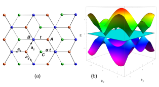
Figure 1: (a) Sketch of the $\alpha$-$T_{3}$ lattice. (b) Band structure of $\alpha$-$T_{3}$ lattice using tight-binding lattice.

The dice lattice can naturally be built by growing trilayers of cubic lattices (e.g. SrTiO₃/SrIrO₃/SrTiO₃) in (111) direction Ran . An optical dice lattice can be produced by a suitable arrangement of three counter-propagating pairs of laser beams Rizzi . The $\alpha$-$T_{3}$ optical lattice can be realized by dephasing one of the pairs of laser beams with respect to other two Raoux ; Rizzi . The Hamiltonian of Hg_1-xCd_xTe quantum well can also be mapped to that of low-energy $\alpha$-T₃ model with effective $\alpha=1/\sqrt{3}$ on appropriate doping Malcolm .

Recently, a list of physical quantities like orbital susceptibility Raoux , optical conductivity Illes ; Illes ; Cserti , magnetotransport properties Tutul ; Malcolm ; Duan ; Firoz , Klein tunneling Urban ; Klein and wave-packet dynamics Tutul1 in $\alpha$-$T_{3}$ lattice have been studied extensively. The Berry phase has become indispensable ingredient in modern condensed matter physics due to its strong influence on magnetic, transport and optical properties Niu-RMP . For example, the variation of the orbital susceptibility with $\alpha$ is a direct consequence of the variable Berry phase of the $\alpha$-T₃ lattice Raoux . It has been pointed out that the quantization of the Hall plataues Tutul ; Malcolm ; Duan and behavior of the SdH oscillation Tutul change with the Berry phase of the $\alpha$-T₃ lattice. The Berry phase dependence of the longitudinal optical conductivity of the $\alpha$-T₃ lattice has also been reported Illes .

In this work, we study quasienergy band structure, time-averaged energy spectrum and time-averaged density of states of $\alpha$-$T_{3}$ lattice irradiated by circularly polarized light. We provide exact and approximate analytical expressions of the quasienergies at the Dirac points as well as at resonant $k$ points for all values of $\alpha$, respectively. The valley degeneracy and the electron-hole symmetry are destroyed by the circularly polarized radiation for $0<\alpha<1$. We establish a direct connection between the quasienergy spectrum and the variable Berry phase, which is responsible for the broken valley degeneracy. The quasienergy gap at the Dirac point decreases with $\alpha$. The behavior of the time-averaged energy and time-averaged density states for $0<\alpha\leq 1$ are appreciably different from that of monolayer graphene.

This paper is organized as follows. In section II, we present preliminary information of the $\alpha$-$T_{3}$ lattice. In section III, we solve Floquet eigensystem for $\alpha$-$T_{3}$ lattice driven by circularly polarized light. In particular, we present numerical and analytical results of quasienergy bands and the corresponding band gaps. In section IV, the results of time-averaged energy spectrum and time-averaged density of states are presented. In section V, we discuss main results of our study.

II Basic information of $\alpha-T_{3}$ lattice

The rescaled tight-binding Hamiltonian of the system considering only nearest neighbour (NN) hopping is given by

$$H_{0}(\textbf{k})=\left(\begin{array}[]{ccc}0&tf^{*}(\textbf{k})\cos\phi&0\\ tf(\textbf{k})\cos\phi&0&tf^{*}(\textbf{k})\sin\phi\\ 0&tf(\textbf{k})\sin\phi&0\end{array}\right)$$ (1)

where $t$ is the NN hopping amplitude, $\alpha$ is parameterized by the angle $\phi$ as $\alpha=\tan\phi$ and $f(\textbf{k})=\sum\limits_{j=1}^{3}\mathrm{e}^{i\bf{k}\cdot{\bf a}_{j}}$. Here, $\bf{a}_{j}$’s are the position vectors of the three nearest neighbors with respect to the rim site. Diagonalising the Hamiltonian gives three energy bands ($E_{\lambda}$) independent of $\alpha$ eucledian : $E_{\pm}(\textbf{k})=\pm t|f(\textbf{k})|$ and $E_{0}(\textbf{k})=0$. Here $\lambda=+1,0,-1$ correspond to the conduction, flat and valence bands, respectively. A unique feature of its band structure is that a flat band $E_{0}({\bf k})$ is sandwiched between two dispersive bands $E_{\pm}({\bf k})$ which have electron-hole symmetry. The nondispersive band also appears in the Lieb Dagotto ; Shen ; Apaja ; Goldman as well as Kagome models Green . Recently, the dispersionless flat band has been engineered in a photonic Lieb lattice formed by a two-dimensional array of optical waveguides Lieb-exp ; Lieb-exp1 . The flat band remains dispersion-less for all values of $\alpha$ and ${\bf k}$. On the other hand, the dispersion of the conduction and valence bands is identical to that of graphene. The full band structure is shown in Fig. 1(b).

The low-energy Hamiltonian around the two inequivalent Dirac points ${\bf K}$ and ${\bf K}^{\prime}$ can be written as

$$H_{0}^{\mu}({\bf k})=\hbar v_{f}{\bf S}(\alpha)\cdot{\bf k},$$ (2)

where $v_{f}=3at/(2\hbar)$, ${\bf k}=\mu k_{x}\hat{\bf x}+k_{y}\hat{\bf y}$ with $\mu=\pm 1$ refers to the K and $\textbf{K}^{\prime}$ valleys, respectively and the components of the spin matrix ${\bf S}(\alpha)$ are defined as

$$S_{x}(\alpha)=\left(\begin{array}[]{ccc}0&\cos\phi&0\\ \cos\phi&0&\sin\phi\\ 0&\sin\phi&0\end{array}\right),$$ (3)

$$S_{y}(\alpha)=\left(\begin{array}[]{ccc}0&-i\cos\phi&0\\ i\cos\phi&0&-i\sin\phi\\ 0&i\sin\phi&0\end{array}\right).$$ (4)

In the vicinity of the two Dirac points, $E_{\pm}(\textbf{k})$ are linear in ${\bf k}$ i.e. $E_{\pm}(\textbf{k})=\pm\hbar v_{f}|\textbf{k}|$, implying massless excitations around the Dirac points, as in the case of graphene.

In contrast to the band structure, the normalized eigen vectors $\psi_{\textbf{k},\lambda}$ depend on $\alpha$ and are given by

$$\psi_{\textbf{k},\pm}=\frac{1}{\sqrt{2}}\left(\begin{array}[]{ccc}\mu\cos\phi e^{-i\mu\theta_{\textbf{k}}}\\ \pm 1\\ \mu\sin\phi e^{i\mu\theta_{\textbf{k}}}\end{array}\right),\psi_{\textbf{k},0}=\left(\begin{array}[]{ccc}\sin\phi e^{-i\mu\theta_{\textbf{k}}}\\ 0\\ -\cos\phi e^{i\mu\theta_{\textbf{k}}}\end{array}\right),$$

where $\theta_{\bf k}=\tan^{-1}(k_{y}/k_{x})$. Moreover, the elements of the spinors from top to bottom represent the probability amplitude of staying in sublattices A (rim), B (hub) and C (rim), respectively. The flat band wavefunction exhibits that the probability amplitude of an electronic wave function centered over the hub sites is always zero. Hence, electrons in the flat band remain localized around the rim sites.

For $\alpha=1$, Eq. (2) reduces to the pseudospin-1 Dirac-Weyl Hamiltonian $H_{0}^{\mu}({\bf k})=\hbar v_{f}\textbf{S}\cdot\textbf{k},$ where $\textbf{S}=(S_{x},S_{y},S_{z})$ are the standard spin-1 matrices.

Berry phase: The topological Berry phase for $\alpha=0$ is simply $\pi$ which is independent of the valleys. For $\alpha>0$, the $\alpha$-dependent Berry phase Illes $\phi_{B}^{\lambda,\mu}$ in the conduction and valence bands is given by

$$\phi_{B}^{\pm 1,\mu}=\pi\mu\cos(2\phi)=\pi\mu\Big{(}\frac{1-\alpha^{2}}{1+\alpha^{2}}\Big{)},$$ (5)

and for the flat band is given by

$$\phi_{B}^{0,\mu}=-2\pi\mu\cos(2\phi)=-2\pi\mu\Big{(}\frac{1-\alpha^{2}}{1+\alpha^{2}}\Big{)}.$$ (6)

Note that the Berry phase is different in the ${\bf K}$ and ${\bf K}^{\prime}$ valleys except for $\alpha=1$. The Berry phase is smoothly decreasing with increase of $\alpha$ and becomes zero at $\alpha=1$. Later, we will show how the Berry phase appears in quasienergy gaps.

III Floquet eigensystem for $\alpha$-$T_{3}$ lattice

We consider a circularly polarized electromagnetic radiation propagating perpendicular to the $\alpha$-$T_{3}$ lattice placed in the $x$-$y$ plane. The corresponding vector potential is given by $\textbf{A}(t)=A_{0}(\cos\omega t\;\hat{\bf x}+\nu\sin\omega t\;\hat{\bf y}),$ where $A_{0}=E_{0}/\omega$ with $E_{0}$ is the amplitude of the electric field and $\omega$ is the frequency of the radiation. Also, $\nu=\pm 1$ denotes counter-clockwise and clockwise rotations of the circularly polarized light, respectively. The frequency of the driving is small compared to the bandwidth of the system. The vector potential satisfies the time periodicity: ${\bf A}(t+T)={\bf A}(t)$ with the time-period $T=2\pi/\omega$. The minimal coupling between the charge carrier and the electric field is obtained through the Peierls substitution: $\hbar{\bf k}\rightarrow(\hbar{\bf k}-q{\bf A}(t))$ with $q=-e$ being the electronic charge. The Hamiltonian for the coupling between the charge carriers and the electromagnetic field can be written as

$$H_{1}^{\mu\nu}(t)=\hbar\omega\beta[S_{-}^{\mu\nu}\mathrm{e}^{i\omega t}+S_{+}^{\mu\nu}\mathrm{e}^{-i\omega t}],$$ (7)

where the $3\times 3$ matrices are $S_{\pm}^{\mu\nu}=\frac{1}{2}[\mu S_{x}(\alpha)\pm i\nu S_{y}(\alpha)]$ and the dimensionless parameter $\beta=eE_{0}l_{\omega}/(\hbar\omega)$ characterizes the strength of the coupling between electromagnetic radiation and charge carrier with $l_{\omega}/a=3\pi t/\hbar\omega\gg 1$ in the THz frequency regime. The dimensionless parameter $\beta$ is less than 1 for the typical intensity of lasers available in the THz frequency regime. In the semiclassical picture, $eE_{0}l_{\omega}$ is the energy gained by the charge carrier while travelling a distance $l_{\omega}$ with the speed $v_{f}$ during one period of the radiation. On the other hand, the charge carrier is dressed with the minimal photon energy $\hbar\omega$.

The total Hamiltonian of a charge carrier near the Dirac point in presence of the electromagnetic radiation is $H^{\mu\nu}({\bf k},t)=H_{0}^{\mu}({\bf k})+H_{1}^{\mu\nu}(t)$ which is periodic in time. By Floquet theory, the solution of time-dependent Schrodinger equation

$$i\hbar\frac{\partial}{\partial{t}}|\psi_{\eta}^{\mu\nu}(\textbf{k},t)\rangle=H^{\mu\nu}(\textbf{k},t)|\psi_{\eta}^{\mu\nu}(\textbf{k},t)\rangle$$ (8)

is given by

$$|\psi_{\eta}^{\mu\nu}(\textbf{k},t)\rangle=\mathrm{e}^{-i\varepsilon_{\eta}^{\mu\nu}(\textbf{k})t/\hbar}|\phi_{\eta}^{\mu\nu}(\textbf{k},t)\rangle.$$ (9)

Here $|\phi_{\eta}^{\mu\nu}(\textbf{k},t)\rangle$ are the time-periodic $1\times 3$ pseudo-spinors and $\varepsilon_{\eta}^{\mu\nu}(\textbf{k})$ are the corresponding quasienergies. There are three independent quasienergy branches along with the three corresponding eigenstates indexed by $\eta=1,0,-1$. Substituting Eq. (9) into Eq. (8), the time-periodic spinor $|\phi_{\eta}^{\mu\nu}(\textbf{k},t)\rangle$ becomes the eigenstate of the Floquet Hamiltonian $H_{F}^{\mu\nu}=H^{\mu\nu}({\bf k},t)-i\hbar\frac{\partial}{\partial t}$ with the eigenvalue $\epsilon_{\eta}^{\mu\nu}(\bf{k})$:

$$\Big{[}H^{\mu\nu}(\textbf{k},t)-i\hbar\frac{\partial}{\partial t}\Big{]}|\phi_{\eta}^{\mu\nu}(\textbf{k},t)\rangle=\epsilon_{\eta}^{\mu\nu}(\bf{k})|\phi_{\eta}^{\mu\nu}(\bf{k},t)\rangle.$$ (10)

Multiplying a phase $\mathrm{e}^{-im\omega t}$ with $m$ being an integer to Eq. (9) and substituting it back to Eq. (10), we obtain

$$(H^{\mu\nu}(\textbf{k},t)-i\hbar\frac{\partial}{\partial t})|\phi_{\eta}^{\mu\nu}(\textbf{k},t)\rangle=(\varepsilon_{\eta}^{\mu\nu}(\textbf{k})+m\hbar\omega)|\phi_{\eta}^{\mu\nu}(\textbf{k},t)\rangle.$$ (11)

This is also an eigenvalue equation as Eq. (10) but with a shifted quasienergy $\varepsilon_{\eta m}^{\mu\nu}(\textbf{k})=\varepsilon_{\eta}^{\mu\nu}(\textbf{k})+m\hbar\omega$. Equations (10) and (11) yield the same Floquet mode, with quasienergies differing by an integer multiple of photon energy $\hbar\omega$. Hence, the index $\eta$ corresponds to a whole class of solutions indexed by $\eta^{\prime}=(\eta,m),m=0,\pm 1,\pm 2,...$ having a discrete spectrum of quasienergies $\varepsilon_{\eta,m}(\textbf{k})$. Thus, a given Floquet state has multiple quasienergy values repeating in the intervals of $\hbar\omega$. For $\alpha$-$T_{3}$ lattice, we have three independent values of quasienergy for a given momentum, which can be attributed to the three independent eigenvalue equations $(\eta=1,0,-1)$. Due to the infinite spectrum without physical distinguishability, the quasienergies can also be confined to a reduced Brillouin zone in energy space with $|\varepsilon_{\eta}^{\mu\nu}(\textbf{k})|<\hbar\omega/2$.

In order to calculate the quasienergies and the corresponding states of the Floquet Hamiltonian, we consider the Fourier expansion of $|\phi_{\eta}^{\mu\nu}(\textbf{k},t)\rangle$

$$|\phi_{\eta}^{\mu\nu}({\bf k},t)\rangle=\sum_{n=-\infty}^{\infty}\mathrm{e}^{-in\omega t}|\chi_{\eta}^{n\mu\nu}({\bf k})\rangle,$$ (12)

which follows from the temporal periodicity of the Floquet mode. Using Eq. (12), the time-dependent differential Eq. (10) reduces to the time-independent eigensystem problem as

$$\sum_{m}\Big{[}H_{0F,mn}^{\mu\nu}+H_{1F,mn}^{\mu\nu}-\epsilon_{\eta}^{\mu\nu}({\bf k})\Big{]}|\chi_{\eta}^{m\mu\nu}({\bf k})\rangle=0,$$ (13)

where the diagonal Floquet Hamiltonian in the Floquet basis is

$$H_{0F,mn}^{\mu\nu}=[\hbar v_{f}{\bf S}(\alpha)\cdot{\bf k}+m\hbar\omega]\delta_{mn}.$$ (14)

and the off-diagonal interaction Hamiltonian

$$H_{1F,mn}^{\mu\nu}=\hbar\omega\beta[S_{-}^{\mu\nu}\delta_{m,n-1}+S_{+}^{\mu\nu}\delta_{m,n+1}]$$ (15)

couples various Fourier modes. Thus, by Floquet matrix theory, we numerically compute the Floquet quasienergies $\varepsilon_{\eta}^{\mu\nu}$ in units of $\hbar\omega$ and the corresponding Floquet states $|\psi_{\eta}^{\mu\nu}(k,t)\rangle$ of the Floquet Hamiltonian $H_{F}^{\mu\nu}$. The following parameters have been used in the numerical calculation: $\omega=2\pi\times 5$ THz, $E_{0}=2$ kV/cm, $v_{f}=10^{6}$ m/s and $\beta=0.3$. Also, $\mu=\nu=+1$ are considered for all the plots unless otherwise stated.

III.1 Exact analytical expressions of quasienergies and band gap at the Dirac points

First, we present exact analytical results of quasienergies and band gaps at the Dirac points. At the Dirac points (${\bf k}=0$), the time-dependent Hamiltonian (in units of $\hbar\omega$) can be written as

$$\bar{H}_{1}^{\mu\nu}(\tilde{t})=\beta[S_{-}^{\mu\nu}e^{i\tilde{t}}+S_{+}^{\mu\nu}e^{-i\tilde{t}}],$$ (16)

where $\tilde{t}=\omega t$.

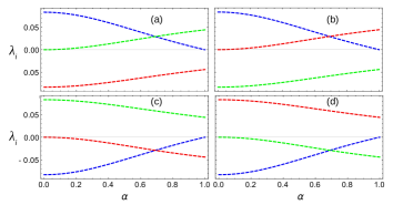
Figure 2: Plots of quasienergies at the Dirac point vs $\alpha$ for various combinations of $\mu$ and $\nu$: (a) $\mu=\nu=1$, (b) $\mu=\nu=-1$, (c) $\mu=1,\nu=-1$, (d) $\mu=-1,\nu=1$. The green, red and blue dotted curves correspond to $\lambda_{1},\lambda_{2}$ and $\lambda_{3}$.

The corresponding Floquet Hamiltonian can be written explicitly as

$$\tilde{H}_{F}^{\mu\nu}(\tilde{t})=\mu\beta\left[\begin{array}[]{ccc}-i\frac{\partial}{\partial\tilde{t}}&\cos\phi\mathrm{e}^{-i\mu\nu\tilde{t}}&0\\ \cos\phi\mathrm{e}^{i\mu\nu\tilde{t}}&-i\frac{\partial}{\partial\tilde{t}}&\sin\phi\mathrm{e}^{-i\mu\nu\tilde{t}}\\ 0&\sin\phi\mathrm{e}^{i\mu\nu\tilde{t}}&-i\frac{\partial}{\partial\tilde{t}}\end{array}\right].$$ (17)

Let us define an unitary operator $\hat{Q}$ given by

$$\hat{Q}=e^{-i\mu\nu({\it I}+S_{z})\tilde{t}},$$ (18)

where ${\it I}$ is the $3\times 3$ identity matrix. By performing the unitary transformation $\hat{Q}^{\dagger}\tilde{H}_{F}^{\mu\nu}(\tilde{t})\hat{Q}$, an effective time-independent Floquet Hamiltonian is obtained

$$\tilde{H}_{F}^{\mu\nu}=\mu\left[\begin{array}[]{ccc}-2\nu&\beta\cos\phi&0\\ \beta\cos\phi&-\nu&\beta\sin\phi\\ 0&\beta\sin\phi&0\end{array}\right].$$ (19)

The zero-momentum quasienergy spectra are given by

$$\lambda_{1} = -\mu\nu+\frac{2\mu}{\sqrt{3}}\sqrt{1+\beta^{2}}\cos\Lambda$$ (20)

$$\lambda_{2} = -\mu\nu-\frac{\mu}{3}\sqrt{1+\beta^{2}}(\sqrt{3}\cos\Lambda+3\sin\Lambda)$$ (21)

$$\lambda_{3} = -\mu\nu-\frac{\mu}{3}\sqrt{1+\beta^{2}}(\sqrt{3}\cos\Lambda-3\sin\Lambda),$$ (22)

where $\Lambda=(1/3)$Arg$[-\xi+\sqrt{\xi^{2}-108(1+\beta^{2})^{3}}]$ and $\xi=27\nu\beta^{2}\big{(}\frac{1-\alpha^{2}}{1+\alpha^{2}}\big{)}$ with Arg$[z]$ gives the argument of the complex number $z$. The corresponding normalized Floquet states are given by

$$|\psi^{\mu\nu}(\tilde{t})\rangle=\frac{\mathrm{e}^{-i(\lambda_{i}+\mu\nu)\tilde{t}}}{\sqrt{1+\beta^{2}\big{(}\frac{\cos^{2}\phi}{(2\mu\nu+\lambda_{i})^{2}}+\frac{\sin^{2}\phi}{\lambda_{i}^{2}}\big{)}}}\left(\begin{array}[]{c}\frac{\beta\cos\phi}{2\mu\nu+\lambda_{i}}\mathrm{e}^{-i\mu\nu\tilde{t}}\\ 1\\ \frac{\beta\sin\phi}{\lambda_{i}}\mathrm{e}^{i\mu\nu\tilde{t}}\end{array}\right).$$ (26)

The parameter $\xi$ can be expressed in terms of the Berry phase given by Eqs. (5) and (6). Thus, the quasienergy is directly related to the Berry phase acquired during a cyclic motion of the charge carriers in presence of a circularly polarized radiation.

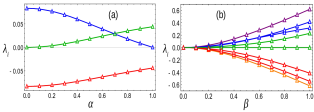
Figure 3: Plots of variation of exact quasienergy at the Dirac point with (a) $\alpha$ for $\beta=0.3$ and (b) $\beta$ for different values of $\alpha$. Exact numerical results are denoted by the triangles. In Fig. (b), the solid green, blue and red lines are for $\alpha=1$, the dotted lines for $\alpha=0.5$ and the purple-orange pair is for $\alpha=0$.

The three Floquet quasienergy branches may be labelled as $(i,m)$, where $i=1,2,3$ represent three branches and $m$ the Floquet index. The corresponding quasienergy $\lambda_{i,m}=\lambda_{i}+m$. The quasienergies of the three branches in the first energy Brillouin zone are given by $\lambda_{1}+\mu(\nu-1),\lambda_{2}+\mu(\nu+1)$ and $\lambda_{3}+\mu\nu$. The three-fold degeneracy at the Dirac point is simply the limiting case ($\beta\rightarrow 0$) of these quasienergies. The variation of these quasienergies with $\alpha$ for $\beta=0.3$ is shown in Fig. 2. Figure 2 displays the photoinduced valley and electron-hole symmetry breaking at the Dirac point for $0<\alpha<1$. The quasienergy variations for the pair having same value of $\mu\nu$ (i.e. $\mu\nu=1$ [Fig. 2(a) and 2(b)] or $\mu\nu=-1$ [Fig. 2(c) and 2(d)]) are identical to each other apart from the interchange of branches. Also, the quasienergy structure for the cases of $\mu\nu=1$ and $\mu\nu=-1$ are inverted copies of each other for $0<\alpha<1$. This implies that spectrum undergoes a flipping on- (i) switching between valleys K and $\textbf{K}^{\prime}$ for a given sense of circular polarization and (ii) changing sense of rotation of the polarization for a given valley. The flipping of quasienergies is trivially symmetric for graphene ($\alpha$=0) and dice lattice ($\alpha$=1) on switching of valleys or polarization.

For $\alpha=0$, the quasienergies within the first energy BZ are obtained as

$$\lambda_{\pm}=\pm\frac{1}{2}(\sqrt{4\beta^{2}+1}-1).$$ (27)

The same results are obtained by Oka and Aoki Oka for irradiated graphene. On the other hand, the quasienergies for the dice lattice ($\alpha=1$) obtained from Eqs. (20,21,22) are $\lambda_{0}=0$ and

$$\lambda_{\pm}=\pm(\sqrt{\beta^{2}+1}-1).$$ (28)

Equations (27) and (28) can be combined to write a general form for quasienergy at the Dirac point as

$$\lambda_{\pm}(S)=\pm(\sqrt{\beta^{2}+S^{2}}-S),$$ (29)

where $S$ is the pseudospin of the underlying lattice. The energy gap at the Dirac point for the pseudospin $S$ is $\Delta_{S}=\lambda_{+}(S)-\lambda_{-}(S)=2(\sqrt{\beta^{2}+S^{2}}-S)$. The energy gap for graphene is $\Delta_{S=\frac{1}{2}}=(\sqrt{4\beta^{2}+1}-1)$ and that for dice lattice is $\Delta_{S=1}=2(\sqrt{\beta^{2}+1}-1)$. It can be easily checked from Fig. 3(a) as well as from Eq. (29) that $\Delta_{S=1}<\Delta_{S=\frac{1}{2}}$. The quasienergy gap at the Dirac point for graphene is higher than that of dice lattice. Thus, the flat band has a shielding effect on the dipole coupling between the electron-photon levels.

In Fig. 3, we show the variation of the three quasienergy branches with $\alpha$ and $\beta$. The colour labeling of Fig. 3 is the same as that of Fig. 2(a). Figure 3(a) shows that our numerical results match very well with the exact results. The quasienergy at the Dirac point increases with the field strength $\beta$ seen at Fig. 3(b).

III.2 Floquet quasienergy branches and band gaps for large values of momentum

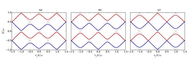
Figure 4: Floquet quasienergy bands for different values of $\alpha$: (a) $\alpha=0$, (b) $\alpha=0.5$, (c) $\alpha=1$.

In this subsection, we present the results obtained by solving the low-energy Floquet Hamiltonian numerically and display the quasienergy band structure within the first two energy Brillouin zones in Fig. 4 for $\alpha=0,0.5$ and 1. The dotted lines indicate the spectrum for zero intensity of radiation, which are identical for all values of $\alpha$. First of all, the quasienergies of the $\alpha$-$T_{3}$ lattice pertaining to different $\eta$ satisfy $\varepsilon_{1}^{\mu\nu}({\bf k})=-\varepsilon_{-1}^{\mu\nu}(\textbf{k})$ for $\alpha=0,1$ and $\varepsilon_{\eta}^{\mu\nu}(\textbf{k})=\varepsilon_{\eta}^{\mu\nu}(-\textbf{k})$ for $0\leq\alpha\leq 1$. The known results of graphene ($\alpha=0$) are reproduced in Fig. 4a. For better visualization, the quasienergy band for $\eta=0$ is shown separately in Fig. 5. The quasienergy branch corresponding to the flat band becomes dispersive mainly around the Dirac and even-photon resonant points for $0<\alpha<1$. This is due to the fact that the flat band states are dressed with integral number of photons in the vicinity of these resonant points, which allows them to mix with dressed conduction and valence band states. The mixing results in dispersion due to shifting of energies of the erstwhile non-dispersive states. On the other hand, the band does not undergo any significant modification at odd-photon resonances, as it cannot be dressed with half-integral number of photons. The dispersion gets completely wiped out at $\alpha=1$. The height of the spikes of the dispersion decreases with increases of the momentum. The band structure gets inverted about the $k$ axis on changing the rotation of electric field vector of the circularly polarized light. The band remains flat for all values of $\alpha$ when applied radiation is linearly polarized. It is to be noted that there is no splitting in the flat band since it does not have any partner band.

Figure 5: Quasienergy band for $\eta=0$ at different values of $\alpha$: (i) $\alpha=0.3$ (green), (ii) $\alpha=0.5$ (red), (iii) $\alpha=0.8$ (purple) and $\alpha=1$ (blue).

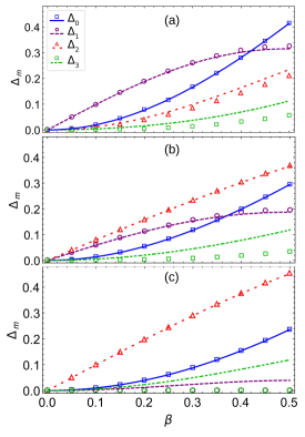
Figure 6: Plots of variation of gaps $\Delta_{m}$ with $\beta$ for (a) $\alpha=0$, (b) $\alpha=0.5$ and (c) $\alpha=1$.

The gaps between the bands ($\eta=\pm 1)$) open up at $k=0$ and at $k_{m}=m\omega/2v_{f}$ with $m=\pm 1,\pm 2,...$. The gap at $k_{m}$ arises due to the AC Stark splitting occurrs due to the multiphoton resonances Gupta ; Home ; Grifoni ; Faisal ; Hsu ; Acosta . There is a set of Bloch states lying on a circle in the vicinity of the Dirac point $k$-space with radius $k_{m}$ such that energy difference between the bands is $m$ multiples of photon energy: $2v_{f}k_{m}=m\omega$. On illumination, new electron-photon states with energy $E_{\lambda}=\hbar v_{f}k_{m}+N_{\lambda}\hbar\omega$ ($\lambda$ band with $N_{\lambda}$ photons) and $E_{\lambda^{\prime}}=-\hbar v_{f}k_{m}+N_{\lambda^{\prime}}\hbar\omega$ with $\lambda^{\prime}\neq\lambda$ ($\lambda^{\prime}$ state with $N_{\lambda^{\prime}}$ photons) are formed. When $E_{\lambda}=E_{\lambda^{\prime}}$ i.e $N_{\lambda}-N_{\lambda^{\prime}}=m\hbar\omega$, the degenerate levels split due to the coupling between the electron and the radiation field and the gap opens up at $k_{m}$. All the gaps tend to diminish at higher values of momentum.

Using the rotating wave approximation (see Appendix), the approximate quasienergies for $\alpha=0$ (for any integer $m$) and $\alpha=1$ (for even $m$) are, respectively, given by

$$(\lambda_{\pm})_{\alpha=0} = \pm\frac{\beta}{2}|J_{m+1}(2\beta)-J_{m-1}(2\beta)|$$ (30)

$$(\lambda_{\pm})_{\alpha=1} = \pm\frac{\beta}{2}|J_{m/2+1}(\beta)-J_{m/2-1}(\beta)|.$$ (31)

From the above expressions, we can see that $(\lambda_{\pm})_{\alpha=0}$ and $(\lambda_{\pm})_{\alpha=1}$ are proportional to the difference between two consecutive integral and even ordered Bessel functions, respectively. The magnitude of the gaps is strongly affected by the argument of the Bessel functions which, for graphene, is twice as that of dice lattice. For $\beta\ll 1$, the asymptotic forms of quasienergy gaps are $(\Delta_{m})_{\alpha=0}\sim\beta^{m}$ and $(\Delta_{m})_{\alpha=1}\sim(\beta/2)^{m/2}$. For weak fields, $(\Delta_{1})_{\alpha=0}$ and $(\Delta_{2})_{\alpha=1}$ vary linearly with $\beta$. The variation of the gaps $\Delta_{m}$ with $\beta$ and $\alpha$ are shown in Fig. 6 and Fig. 7, respectively. The curves represent the numerical results while their corresponding markers represent the results obtained from exact analytical expressions ($\Delta_{0}$) and rotating wave approximation ($\Delta_{1},\Delta_{2},\Delta_{3}$). All the gaps increase monotonically with $\beta$. Moreover, $\Delta_{0}$ (solid blue) and $\Delta_{1}$ (dashed purple) get reduced at higher $\alpha$. In contrast, $\Delta_{2}$ (dotted red) is found to increase with $\alpha$. The gap $\Delta_{3}$ (dashed-dotted green) increases very slowly with $\alpha$. The splitting at even-photon resonant points is affected by the intervention of the flat band dressed with integral number of photons. The interplay of the three bands results in a increase in magnitude of the gap as $\alpha$ increases. We see that the agreement between numerical and analytical results does not hold good at higher momentum.

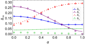
Figure 7: Plots of variation of gaps $\Delta_{m}$ with $\alpha$ for $\beta=0.3$.

IV Time-averaged energies and density of states

In this section, we discuss about time-averaged quantities such as mean energy and the corresponding density of states. The mean energy is a single-valued quantity, which is independent of the choice of the quasienergy of the Floquet state. The mean energy helps to understand whether the Floquet states are occupied or unoccupied Gupta ; Faisal ; Hsu . For example, the Floquet states having lower mean quasienergy will be accommodated first. Also, the mean quasienergy can be used to characterize whether the state is electron-like or hole-like Wu .

Time-averaged energies: The expectation value of the Hamiltonian in a Floquet state is a periodic function of time. This helps us to formulate the energy averaged over a full cycle of a periodic driving and is given by

$$\bar{E_{\eta}^{\mu\nu}}(\textbf{k})=\frac{1}{T}\int_{0}^{T}\langle\psi_{\eta}^{\mu\nu}(\textbf{k},t)|H^{\mu\nu}(\textbf{k},t)|\psi_{\eta}^{\mu\nu}(\textbf{k},t)\rangle dt.$$ (32)

Incorporating the Fourier series (Eq. (12)) into the above equation, we get

$$\bar{E}_{\eta}^{\mu\nu}(\textbf{k})=\varepsilon_{\eta}^{\mu\nu}(\textbf{k})+\sum_{n=-\infty}^{\infty}n\hbar\omega\langle\chi_{\eta}^{n\mu\nu}(\textbf{k})|\chi_{\eta}^{n\mu}(\textbf{k})\rangle.$$ (33)

Hence, the averaged energy can be viewed as the weighted average of energies possessed by the Fourier harmonics of the Floquet modes.

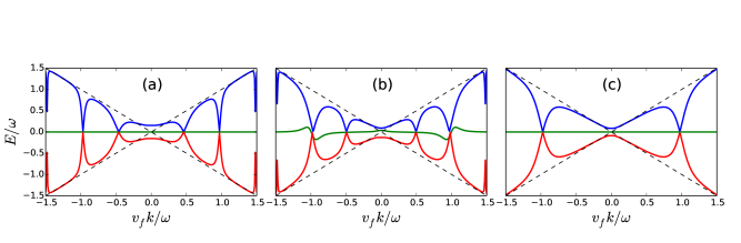
Figure 8: Time-averaged energy of the three Floquet branches for (a) $\alpha=0$, (b) $\alpha=0.5$, (c) $\alpha=1$.

The time-averaged energy (around ${\bf K}$ valley) corresponding to the Floquet states of the three branches for different values of $\alpha$ are shown in Fig. 8. The blue, green and red bands represent the quasielectron, flat band and quasihole states respectively. For $0<\alpha<1$, the mean energy band structure around ${\bf K}^{\prime}$ can be obtained by simply inverting the same for ${\bf K}$ valley. Due to absence of inversion symmetry of the band structure for $0<\alpha<1$, the valley degeneracy is broken. As $\beta\rightarrow 0$, we obtain the field-free Dirac cones shown by the dotted lines. For $0\leq\alpha<1$, the mean energy goes to zero near one-photon and two-photon resonant points due to crossover between quasielectron and quasihole states Wu . The vanishing of mean energies at these resonant points is also observed for $\alpha<1$. But, dice lattice has a non-zero mean energy near $one$-$photon$ resonance. This can be attributed to the fact that the gap at $one$-$photon$ resonance becomes vanishingly small and mimics the radiation-free case for $\alpha=1$. A finite gap exists at the Dirac point for all values of $\alpha$. The three-fold degeneracy at the Dirac point is lifted by the radiation. Careful examination reveals that the symmetric nature of $\eta=\pm 1$ bands (electron-hole symmetry) is slightly disrupted near the Dirac point for $0<\alpha<1$. The symmetry is restored at $\alpha=1$. A distortion occurs in the mean energy spectrum of the flat band at $k=0,\pm\omega/v_{f}$, similar to that obtained in the quasienergy spectrum. The distortions flatten out at $\alpha=1$.

Time-averaged density of states: The time-averaged density of states over a driving cycle is defined as

$$D(E)=g_{s}\sum_{n,\eta,\mu,\textbf{k}}\langle\chi_{\eta}^{n}(\textbf{k})|\chi_{\eta}^{n}(\textbf{k})\rangle\delta\big{(}E-(\varepsilon_{\eta}(\textbf{k})+n\hbar\omega)\big{)}$$ (34)

Here, the factor $g_{s}=2$ appears due to the spin degeneracy. On converting the sum over k to integral, i.e $\sum\limits_{\textbf{k}}\rightarrow\frac{1}{(2\pi)^{2}}\int^{\textbf{k}}d^{2}\textbf{k}$ and using the azimuthal symmetry of quasienergy band structure for circularly polarized light, we get the density of states per unit area as

$$g(E)=D_{0}\sum\limits_{\eta,n,\mu}\int_{0}^{\infty}\langle\chi_{\eta}^{n\mu}(\tilde{k})|\chi_{\eta}^{n\mu}(\tilde{k})\rangle\delta(\tilde{\varepsilon}-(\tilde{\varepsilon}_{\eta}^{\mu}(\tilde{k})+n))\tilde{k}d\tilde{k}$$ (35)

where $D_{0}=g_{s}\omega/(2\pi\hbar v_{f}^{2})=1.515\times$ 10¹³ meV^-1 m^-2. $\tilde{\varepsilon}$ and $\tilde{\varepsilon}_{\eta}^{\mu}(\tilde{k})$ are the dimensionless quasienergies such that $E=\tilde{\varepsilon}\hbar\omega$. Using the property of the Dirac-delta function, the above integral can be further simplified as

$$g(E)=D_{0}\sum_{\gamma,\tilde{k}_{i}^{(\gamma)}(\tilde{\varepsilon})}\frac{\langle\chi_{\eta}^{n\mu}(\tilde{k}_{i}^{(\gamma)}(\tilde{\varepsilon})|\chi_{\eta}^{n\mu}(\tilde{k}_{i}^{(\gamma)}(\tilde{\varepsilon})\rangle\tilde{k}_{i}^{(\gamma)}(\tilde{\varepsilon})}{|\tilde{\varepsilon}_{\eta}^{\prime}(\tilde{k}_{i}^{(\gamma)}\tilde{\varepsilon})|}$$ (36)

where $\gamma=\{n,\eta,\mu\}$ is a set of quantum numbers and $\tilde{k}_{i}^{(\gamma)}(\tilde{\varepsilon})$ is the $i$-th positive root of $\tilde{\varepsilon}-(\tilde{\varepsilon}_{\eta}^{\mu}(\tilde{k})+n)=0$ for a given $n$.

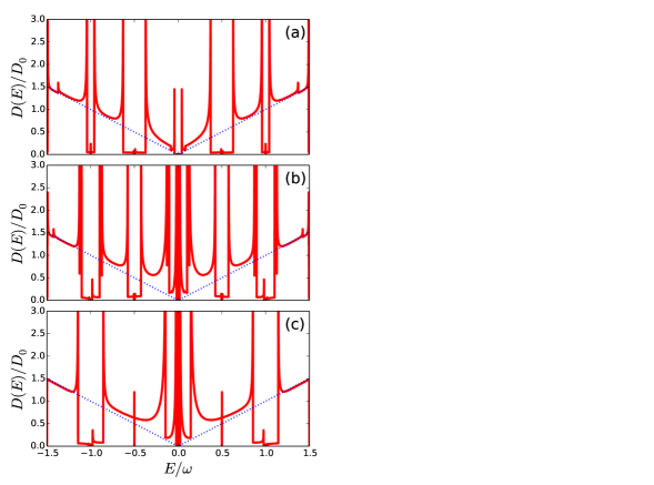
Figure 9: Time-averaged density of states of quasielectron and quasihole states for (a) $\alpha=0$, (b) $\alpha=0.5$, (c) $\alpha=1$.

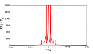
Figure 10: Time-averaged density of states of quasiflat band around the Dirac point for $\alpha=0.5$.

Time-averaged density of states of electronlike and holelikes quasienergy bands for three different values of $\alpha$ is shown in Fig. 9. Figure 9(a) shows the DOS for $\alpha=0$, which is similar to the results obtained by other groups Oka ; Wu . The peaks represent the Van Hove singularities occuring due to the extrema in the quasienergy band structure. Apart from large peaks, there are spikes around $E=\pm\omega/2$ and $E=\pm\omega$ with vanishingly small DOS. This is because of the photoinduced gaps at the boundaries of the energy Brillouin zones. A small but finite contribution of DOS in these energy ranges appears due to closing of gaps at higher momenta. Additional peaks are born at the Dirac point for finite $0<\alpha\leq 1$ as seen in Figs. 9(b) and 9(c). The separation between the peaks centred around $E=\pm\omega/2$ decreases with $\alpha$, while that around $E=\pm\omega$ increases with $\alpha$. This is related to the fact that $\Delta_{1}(\Delta_{2})$ decreases (increases) with $\alpha$.

The time-averaged DOS for the flat band quasienergy around the Dirac point is shown in Fig. 10. Since the regions between two consecutive even-photon resonant points are predominantly flat, a large peak appears at zero energy. The dispersion at even-photon resonant points in the flat band lead to occurence of additional peaks symmetrically placed around around the peak at zero energy. Similar feature in the DOS is repeated at energies equal to integral multiples of photon energy. In dice lattice, only central peaks are present at $N\hbar\omega$ ($N$ being the integer) due to absence of dispersion in the flat band.

V Summary and Conclusion

We have investigated the Floquet quasienergy spectrum numerically and analytically for the $\alpha$-$T_{3}$ lattice driven by circularly polarized radiation. Exact analytical expressions of the quasienergy at the Dirac points for all values of $\alpha$ and field strength are provided. The band gap at the Dirac point appears due to the circularly polarized radiation for all values of $\alpha$. The quasienergy gap at the Dirac point decreases with the increase of $\alpha$. Within the rotating wave approximation, we are able to get approximate expressions of quasienergy at single-photon and multi-photon resonant points. Approximate results match very well with the numerical results based on Floquet method. The expressions reveal that the quasienergy is directly related to the Berry phase acquired during a cyclic motion driven by the rotating electric field. The valley symmetry is broken due to different Berry phase for different valleys for $0<\alpha<1$. The quasienergy flat band remains dispersionless in presence of radiation for dice lattice. However, dispersive spikes appear in and around the Dirac and even-photon resonant points for $0<\alpha<1$. The mean energy is non-vanishing around single-photon resonance point for dice lattice unlike $\alpha<1$. In contrast to graphene, we find that additional peaks appear in the time-averaged density of states at the Dirac point for $0<\alpha\leq 1$. The pattern of the DOS near the single-photon and two-photon resonant points varies significantly with $\alpha$.

Floquet-Bloch states on the surface of a topological insulator have been observed using time- and angle-resolved photoemission spectroscopy (TrARPES)TI-exp . There is a possibility that the quasienergy band structure of the $\alpha$-T₃ lattice may be probed using TrARPES on subjecting the lattice to intense microwave pulses perpendicular to the lattice plane. The variation in quasienergy band gaps with $\alpha$ may be observed by modulating the phase of one of the three counter-propagating laser beams. Similarly, the quasienergy band structure for $\alpha=1/\sqrt{3}$ may be verified by devising suitable means to irradiate Hg_1-xCd_xTe quantum wells. The radiation-dressed band structure of such systems may open up doors for new opto-electronic devices.

VI Acknowledgement

We would like to thank Firoz Islam and Sonu Verma for useful discussions.

VII APPENDIX

VII.1 Analytical results within rotating wave approximation

In this appendix, we shall derive analytical expressions of the quasienergy branches within rotating wave approximation Wu . The analytical expressions help us to understand the Berry phase dependency of the quasienergy bands and band gaps.

The time-periodic Hamiltonian $H^{\mu\nu}({\bf k},t)$ can be transformed in the basis formed by the eigenvectors of the low-energy Hamiltonian $H_{0}^{\mu}(\textbf{k})$ with the help of the unitary operator $\hat{U}_{\textbf{k}}$ given by

$$\hat{U}_{\textbf{k}}=\frac{1}{\sqrt{2}}\left(\begin{array}[]{ccc}\mu\cos\phi e^{-i\mu\theta_{\textbf{k}}}&\sqrt{2}\sin\phi e^{-i\mu\theta_{\textbf{k}}}&\mu\cos\phi e^{-i\mu\theta_{\textbf{k}}}\\ 1&0&-1\\ \mu\sin\phi e^{i\mu\theta_{\textbf{k}}}&-\sqrt{2}\cos\phi e^{i\mu\theta_{\textbf{k}}}&\sin\phi e^{i\mu\theta_{\textbf{k}}}\end{array}\right).$$

The transformed Hamiltonian $\hat{U}_{\textbf{k}}^{\dagger}H^{\mu\nu}(\textbf{k},t)\hat{U}_{\textbf{k}}=\tilde{H}^{\mu\nu}(\textbf{k},t)$ reads as

$$\tilde{H}^{\mu\nu}(\textbf{k},t)=\hbar\omega\Big{[}\frac{v_{f}k}{\omega}S_{z}+\tilde{H}_{\rm intra}(t)+\tilde{H}_{\rm inter}(t)\Big{]},$$ (37)

where $\tilde{H}_{\rm intra}(t)=\beta(\cos\mu\theta_{k}\cos\omega t+\mu\nu\sin\mu\theta_{k}\sin\omega t)S_{z}$ with $S_{z}$ being the $z$-component of the spin-1 matrix and

$$\tilde{H}_{\rm inter}(t)=\frac{if(t)}{\sqrt{2}} \left[\begin{array}[]{ccc}0&\sin 2\phi&\sqrt{2}\mu\cos 2\phi\\ -\sin 2\phi&0&\sin 2\phi\\ -\sqrt{2}\mu\cos 2\phi&-\sin 2\phi&0\end{array}\right]$$ (38)

where $f(t)=\beta(\nu\cos\mu\theta_{k}\sin\omega t-\mu\sin\mu\theta_{k}\cos\omega t)$.

The Schrodinger equation is then given by

$$\Big{[}\frac{i}{\omega}\partial_{t}-\big{(}\frac{v_{f}k}{\omega}S_{z}+\tilde{H}_{\rm intra}(t)+\tilde{H}_{\rm inter}(t)\big{)}\Big{]}|\psi_{\eta}({\bf k},t)\rangle=0.$$ (39)

We solve the Schrodinger equation by omitting the interband term $\tilde{H}_{\rm inter}(t)$ and get the following solutions:

$$|\psi_{+1}^{(0)}({\bf k},t)\rangle=e^{-iv_{f}kt}u(\theta_{\textbf{k}},t)\left(\begin{array}[]{ccc}1\\ 0\\ 0\end{array}\right)$$ (40)

$$|\psi_{-1}^{(0)}({\bf k},t)\rangle=e^{iv_{f}kt}u^{*}(\theta_{\textbf{k}},t)\left(\begin{array}[]{ccc}0\\ 0\\ 1\end{array}\right)$$

$$|\psi_{0}^{(0)}({\bf k},t)\rangle=\left(\begin{array}[]{ccc}0\\ 1\\ 0\end{array}\right)$$

where $u\big{(}\theta_{\textbf{k}},t)=\exp(i\beta[-\cos\mu\theta_{\textbf{k}}\sin\omega t+\mu\nu\sin\mu\theta_{\textbf{k}}(\cos\omega t-1)])$. Note that $u\big{(}\theta_{\textbf{k}},t)$ is also a time-periodic function. The quasienergy of $\psi_{({\bf k},\eta)}^{(0)}(t)$ is exactly the same as the zero field case. It tells us that all the quasienergy gaps appear due to the interband term $\tilde{H}_{\rm inter}(t)$.

Let the solution of Eq. (39) be of the form:

$$|\psi_{\eta}({\bf k},t)\rangle=\sum\limits_{\gamma=-1}^{1}a_{\eta,\gamma}(t)|\psi_{\gamma}^{(0)}({\bf k},t)\rangle,$$

we get

$$\partial_{t}a_{\eta,1}(t) = \frac{\omega}{\sqrt{2}}\Big{[}\sqrt{2}\mu\cos 2\phi\;a_{\eta,-1}(t)e^{2iv_{f}kt}[u^{*}(\theta_{\textbf{k}},t)]^{2}+\sin 2\phi\;e^{iv_{f}kt}u^{*}(\theta_{\textbf{k}},t)a_{\eta,0}(t)\Big{]}f(t)$$ (41)

$$\partial_{\bar{t}}a_{\eta,0}(t) = \frac{\omega}{\sqrt{2}}\Big{[}-a_{\eta,1}(t)e^{-iv_{f}kt}u(\theta_{\textbf{k}},t)+a_{\eta,-1}(t)e^{iv_{f}kt}u^{*}(\theta_{\textbf{k}},t)\Big{]}\sin 2\phi\;f(t)$$ (42)

$$\partial_{\bar{t}}a_{\eta,-1}(t) = -\frac{\omega}{\sqrt{2}}\Big{[}\sqrt{2}\mu\cos 2\phi\;a_{\eta,1}(t)e^{-2iv_{f}kt}[u(\theta_{\textbf{k}},t)]^{2}+\sin 2\phi\;e^{-iv_{f}kt}u(\theta_{\textbf{k}},t)a_{\eta,0}(t)\Big{]}\;f(t).$$ (43)

Taking $(\beta\omega/\sqrt{2})y_{l}(\theta_{k})$ and $(\beta\omega/\sqrt{2})z_{l}(\theta_{k})$ as the discrete Fourier transform of the periodic functions $[u(\theta_{\textbf{k}},t)]^{2}f(t)$ and $u(\theta_{\textbf{k}},t)f(t)$ respectively, we have

$$\partial_{t}a_{\eta,1}(t) = \frac{\beta\omega}{2}\Big{[}\sqrt{2}\cos 2\phi\;a_{\eta,-1}(t)\sum_{l=-\infty}^{\infty}y_{l}^{*}(\theta_{k})e^{i(2v_{f}k-l\omega)t}+\sin 2\phi\;a_{\eta,0}(t)\sum_{l=-\infty}^{\infty}z_{l}^{*}(\theta_{k})e^{i(v_{f}k-l\omega)t}\Big{]}$$ (44)

$$\partial_{t}a_{\eta,0}(t) = \frac{\beta\omega}{2}\Big{[}-a_{\eta,1}(t)\sum_{l=-\infty}^{\infty}z_{l}(\theta_{k})e^{-i(v_{f}k-l\omega)t}+a_{\eta,-1}(t)\sum_{l=-\infty}^{\infty}z_{l}^{*}(\theta_{k})e^{i(v_{f}k-l\omega)t}\Big{]}\sin 2\phi$$ (45)

$$\partial_{t}a_{\eta,-1}(t) = -\frac{\beta\omega}{2}\Big{[}\sqrt{2}\cos 2\phi\;a_{\eta,1}(t)\sum_{l=-\infty}^{\infty}y_{l}(\theta_{k})e^{-i(2v_{f}k-l\omega)t}+\sin 2\phi\;a_{\eta,0}(t)\sum_{l=-\infty}^{\infty}z_{l}(\theta_{k})e^{-i(v_{f}k-l\omega)t}\Big{]}.$$ (46)

Here

$$z_{l}(\theta_{k}) = \frac{1}{\sqrt{2}}\Big{[}u_{l+1}^{(1)}(\theta_{k})(-\mu\sin\mu\theta_{k}+i\nu\cos\mu\theta_{k})$$ (47)

$$- u_{l-1}^{(1)}(\theta_{k})(\mu\sin\mu\theta_{k}+i\nu\cos\mu\theta_{k})\Big{]}$$

and

$$y_{l}(\theta_{k}) = \frac{1}{\sqrt{2}}\Big{[}u_{l+1}^{(2)}(\theta_{k})(-\mu\sin\mu\theta_{k}+i\nu\cos\mu\theta_{k})$$ (48)

$$- u_{l-1}^{(2)}(\theta_{k})(\mu\sin\mu\theta_{k}+i\nu\cos\mu\theta_{k})\Big{]},$$

where $u_{l}^{(j)}(\theta_{k})$ with ($j=1,2)$ is defined as

$$u_{l}^{(j)}(\theta_{k})=\frac{1}{T}\int_{0}^{T}[u(\theta_{\textbf{k}},t)]^{j}e^{-il\omega t}dt.$$ (49)

The exact expressions of $u_{l}^{(1)}(\theta_{k})$ and $u_{l}^{(2)}(\theta_{k})$ are obtained as

$$u_{l}^{(1)}(\theta_{k}) = e^{-i\mu\nu\beta\sin\mu\theta_{k}}J_{l}(2|p(\theta_{k})|)\bigg{(}\frac{-p(\theta_{k})}{|p(\theta_{k})|}\bigg{)}^{l}$$ (50)

$$u_{l}^{(2)}(\theta_{k}) = e^{-i2\mu\nu\beta\sin\mu\theta_{k}}J_{l}(2|q(\theta_{k})|)\bigg{(}\frac{-q(\theta_{k})}{|q(\theta_{k})|}\bigg{)}^{l},$$ (51)

where $J_{l}(x)$ is the $l$-th order Bessel fuction, $p(\theta_{k})=\frac{\beta}{2}(\cos\mu\theta_{k}-i\mu\nu\sin\mu\theta_{k})$ and $q(\theta_{k})=\beta(\cos\mu\theta_{k}-i\mu\nu\sin\mu\theta_{k})$. It is not possible to solve Eqs. (44), (45), and (46) in closed analytical form. However, owing to the high frequency of radiation, standard rotating wave approximation (RWA) can be used to obtain closed form expressions.

There are two frequency detuning terms namely $\delta_{1}=2v_{f}k-m\omega$ and $\delta_{2}=v_{f}k-m\omega$, due to presence of an additional dispersionless band. Near the resonance points, $(\delta_{1,2}\simeq 0)$, the momentum values $\textbf{{k}}_{m}$ are such that the energy difference between the bands equals $m$ multiples of photon energy $\hbar\omega$.

For even $m$ (excluding 0), the terms $y_{m}(\theta_{k})$ and $z_{m/2}(\theta_{k})$ are retained in their respective series. But, for odd integer $m$, we see that retaining the $m$-th term from $y_{l}(\theta_{k})$ series allots $v_{f}k/\omega$ an odd integer value. So within RWA, all the terms in the $z_{l}(\theta_{k})$ series will be rapidly oscillating, allowing us to discard this series altogether. Hence, for odd $m$, we retain only $y_{m}(\theta_{k})$. This leads to two distinct cases for even and odd integers, each of which produces separate systems of coupled differential equations for the determination of Floquet quasienergies.

Case I: For even $m$ case, Eqs. (44), (45) and (46) become

$$\partial_{t}a_{\eta,1}(t) = \frac{\beta\omega}{2}\Big{[}\sqrt{2}\mu\cos 2\phi\;a_{\eta,-1}(t)y_{m}^{*}(\theta_{k})e^{i\delta_{1}t}+\sin 2\phi\;a_{\eta,0}(t)z_{m/2}^{*}(\theta_{k})e^{i\delta_{2}t}\Big{]}$$ (52)

$$\partial_{t}a_{\eta,0}(t) = \frac{\beta\omega}{2}\Big{[}-a_{\eta,1}(t)z_{m/2}(\theta_{k})e^{-i\delta_{2}t}+a_{\eta,-1}(t)z_{m/2}^{*}(\theta_{k})e^{i\delta_{2}t}\Big{]}\;\sin 2\phi$$ (53)

$$\partial_{t}a_{\eta,-1}(t) = -\frac{\beta\omega}{2}\Big{[}\sqrt{2}\mu\cos 2\phi\;a_{\eta,1}(t)y_{m}(\theta_{k})e^{-i\delta_{1}t}+\sin 2\phi\;a_{\eta,0}(t)z_{m/2}(\theta_{k})e^{-i\delta_{2}t}\Big{]}.$$ (54)

Note that Eq. (53) is redundant for $\alpha=0$ case. Equations (52) and (54) with $\alpha=0$ reproduce all the approximate analytical results for graphene provided by Zhou and Wu Wu .

Furthermore, the above set of equations can not be solved analytically unless we solve it on exact resonance i.e. $\delta_{1}=\delta_{2}=0$. On exact resonance condition, the approximate expressions of quasienergies for $0<\alpha<1$ obtained from Eqs. (52), (53) and (54) are $\lambda_{0}=0$ and

$$\lambda_{\pm}=\pm\frac{\beta}{\sqrt{2}}\sqrt{\cos^{2}2\phi|y_{m}(\theta_{\textbf{k}})|^{2}+\sin^{2}2\phi|z_{m/2}(\theta_{\textbf{k}})|^{2}}$$ (55)

From the above expression, we see that the quasienergy is proportional to root mean modulus squared of the coupling parameters $y_{m}(\theta_{\textbf{k}})$ and $z_{m/2}(\theta_{\textbf{k}})$ weighted by terms dependent on Berry phase ($\sim\cos 2\phi$) of the system. The sum of the weights is unity for all $\alpha$. Since the Berry phase varies smoothly from $\pi$ to 0 as $\alpha$ goes 0 to 1, the weight of $y_{m}(\theta_{\textbf{k}})$ decreases while that of $z_{m/2}(\theta_{\textbf{k}})$ increases with $\alpha$. The quasieigenenergy for special cases like $\alpha=0$ and $\alpha=1$ can be obtained easily. For $\alpha=0$, $\lambda_{\pm}=\pm\frac{\beta}{\sqrt{2}}|y_{m}(\theta_{\textbf{k}})|$. This is the same result as obtained for monolayer graphene Wu . On the other hand, for dice lattice ($\alpha=1$), we get $\lambda_{\pm}=\pm\frac{\beta}{\sqrt{2}}|z_{m/2}(\theta_{\textbf{k}})|$ and $\lambda_{0}=0$. For the dice lattice, the quasienergy gap between $\eta=\pm 1$ at the resonance point is

$$\Delta_{m}(\theta_{\bf k})=\sqrt{2}\beta|z_{m/2}(\theta_{\textbf{k}})|.$$ (56)

The magnitude of the gap in graphene and dice lattice depends on the effective coupling parameters $|y_{m}(\theta_{\textbf{k}})|$ and $|z_{m/2}(\theta_{\textbf{k}})|$, respectively. The behaviour of the gap in graphene and dice lattice is quite different.

Case II: For odd $m$, Eqs. (44), (45) and (46) can be approximated as

$$\partial_{t}a_{\eta,1}(t) \approx \frac{\beta\omega\mu}{\sqrt{2}}\cos 2\phi\;a_{\eta,-1}(t)y_{m}^{*}(\theta_{k})e^{i\delta_{1}t}$$ (57)

$$\partial_{t}a_{\eta,0}(t) \approx 0$$ (58)

$$\partial_{t}a_{\eta,-1}(t) \approx -\frac{\beta\omega\mu}{\sqrt{2}}\cos 2\phi\;a_{\eta,1}(t)y_{m}(\theta_{k})e^{-i\delta_{1}t}.$$ (59)

Thus for odd $m$, we obtain simplified expression of quasienergy for a given $\alpha$:

$$\lambda_{\pm}\approx\pm\frac{\beta}{\sqrt{2}}|y_{m}(\theta_{\textbf{k}})|\Big{(}\frac{1-\alpha^{2}}{1+\alpha^{2}}\Big{)}$$ (60)

and $\lambda_{0}=0$. Interestingly, it shows that the gap with odd values of $m$ closes in the dice lattice, which is in sharp contrast with the graphene case. Although Eq. (60) shows that $\Delta_{m}=0$ for $\alpha=1$, but this is not the case. We will get a small non-zero value of $\Delta_{m}$ on taking into account the higher-order contribution from Eqs. (44), (45) and (46).

The quasienergy gap is essentially determined by the Berry phase and two coupling parameters $|y_{m}(\theta_{\textbf{k}})|$ and $|z_{m/2}(\theta_{\textbf{k}})|$. The expressions of the coupling parameters can be simplified further by setting $\theta_{\bf k}=0$ since the quasienergy spectrum is isotropic for all values of $\alpha$ for circularly palarized light. On substitution $\theta_{\bf k}=0$ into Eqs. (47) and (48), we get

$$y_{l}(0) = \frac{i\nu}{\sqrt{2}}(-1)^{l}[J_{l-1}(2\beta)-J_{l+1}(2\beta)]$$ (61)

$$z_{l}(0) = \frac{i\nu}{\sqrt{2}}(-1)^{l}[J_{l-1}(\beta)-J_{l+1}(\beta)].$$ (62)

Thus, the approximate forms of quasienergies for $\alpha=0$ (for any integer $m$) and $\alpha=1$ (for even $m$) turn out to be

$$(\lambda_{\pm})_{\alpha=0} = \pm\frac{\beta}{2}|J_{m+1}(2\beta)-J_{m-1}(2\beta)|,$$ (63)

$$(\lambda_{\pm})_{\alpha=1} = \pm\frac{\beta}{2}|J_{m/2+1}(\beta)-J_{m/2-1}(\beta)|.$$ (64)

For weak field ($\beta\ll 1$), the asymptotic forms of quasienergy gaps are obtained from the above expressions as

$$(\Delta_{m})_{\alpha=0} \sim \frac{\beta^{m}}{(m-1)!}\hskip 2.84544pt{\rm and}\hskip 2.84544pt(\Delta_{m})_{\alpha=1}\sim\frac{2(\beta/2)^{m/2}}{(m/2-1)!}.$$ (65)

References

- (1) P. Hanggi, Quantum Transport and Dissipation (Wiley, New York, 1988), Chap. 5.
- (2) A. Eckardt and E. Anisimova, New J. Phys. 17, 093039 (2015)
- (3) M. V. Fistul and K. V. Efetov, Phys. Rev. Lett. 98, 256803 (2007)
- (4) S. V. Syzranov, M. V. Fistul, and K. V. Efetov, Phys. Rev. B 78, 045407 (2008)
- (5) F. J. Lopez-Rodriguez and G. G. Naumis, Phys. Rev. B 78, 201406(R) (2008)
- (6) T. Oka and H. Aoki, Phys. Rev. B 79, 081406(R) (2009)
- (7) T. Oka and H. Aoki, J. Phys.: Conf. Ser. 200, 062017 (2010)
- (8) W. Zhang, P. Zhang, S. Duan, and Xian-geng Zhao New J. Phys. 11, 063032 (2009)
- (9) O. V. Kibis, Phys. Rev. B 81, 165433 (2010)
- (10) Y. Zhou and M. W. Wu, Phys. Rev. B 83, 245436 (2011)
- (11) A. Scholz, A. Lopez, and J. Schliemann, Phys. Rev. B 83, 245436 (2011)
- (12) A. K. Gupta, O. E. Alon, and N. Moiseyev, Phys. Rev. B 68, 205101 (2003)
- (13) M. Ezawa, Phys. Rev. Lett. 110, 026603 (2013)
- (14) A. Lopez, A. Scholz, B. Santos, and J. Schliemann, Phys. Rev. B 91, 125105 (2015)
- (15) M. I. Katsnelson, Graphene: Carbon in two dimensions (Cambridge University Press, 2012)
- (16) B. Sutherland, Phys. Rev. B 34, 5208 (1986)
- (17) J. Vidal, R. Mosseri, and B. Doucot, Phys. Rev. Lett. 81, 5888 (1998)
- (18) S. E. Korshinov, Phys. Rev. B 63, 134503 (2001)
- (19) M. Rizzi, V. Cataudella, and R. Fazio, Phys. Rev. B 73, 144511 (2006)
- (20) D. F. Urban, D. Bercioux, M. Wimmer, and W. Haussler, Phys. Rev. B 84, 115136 (2011)
- (21) J. D. Malcolm and E. J. Nicol Phys. Rev. B 93, 165433 (2016)
- (22) D. Bercioux, D. F. Urban, H. Grabert, and W. Hausler, Phys. Rev. A 80, 063603 (2009)
- (23) M. Vigh, L. Oroszlány, S. Vajna, P. San-Jose, G. Dávid, J. Cserti, and Balázs Dora, Phys. Rev. B 88, 161413(R), (2013)
- (24) A. Raoux, M. Morigi, J-N. Fuchs, F. Piechon, and G. Montambaux, Phys. Rev. Lett. 112, 026402 (2014)
- (25) F. Wang and Y. Ran, Phys. Rev. B 84, 241103 (2011)
- (26) J. D. Malcolm and E. J. Nicol, Phys. Rev. B 92, 035118 (2015)
- (27) E. Illes, J. P. Carbotte, and E. J. Nicol, Phys. Rev. B 92, 245410 (2015)
- (28) E. Illes and E. J. Nicol, Phys. Rev. B 94, 125435 (2016)
- (29) A. D. Kovacs, G. David, B. Dora, and J. Cserti, Phys. Rev. B 95, 035414 (2017)
- (30) T. Biswas and T. K. Ghosh, J. Phys.: Condens. Matter 28, 495302 (2016)
- (31) D. Xiao, M. C. Chang, and Q. Niu, Rev. Mod. Phys. 82, 1959 (2010)
- (32) J. D. Malcolm and E. J. Nicol, Phys. Rev. B 92, 035118 (2015)
- (33) Y. Xu and L.-M. Duan, Phys. Rev. B 96, 155301 (2017)
- (34) SK Firoz Islam and P. Dutta, Phys. Rev. B 96, 045418 (2017)
- (35) E. Illes and E. J. Nicol, Phys. Rev. B 95, 235432 (2017)
- (36) T. Biswas and T. K. Ghosh, J. Phys.: Condens. Matter 30, (2018) 075301
- (37) The eigen spectrum of unscaled Hamiltonian is . For a fixed k, is determined by the points in two-dimensional Euclidean parameter space of hopping amplitudes and . Since is proportional to , the spectrum will be invariant for all points lying on a circle of fixed radius centred at origin. Rescaling the Hamiltonian by is equivalent to parametrizing the hopping amplitudes as and such that . As a result, variation of or traces out the points on a circle of radius in the parameter space such that the eigenvalues are independent of .
- (38) E. Dagotto, E. Fradkin, and A. Moreo, Phys. Lett. B 172, 383 (1986)
- (39) R. Shen, L. B. Shao, B. Wang, and D. Y. Xing, Phys. Rev. B 81, 041410(R) (2010)
- (40) V. Apaja, M. Hyrkäs, and M. Manninen, Phys. Rev. A 82, 041402(R) (2010)
- (41) N. Goldman, D. F. Urban, and D. Bercioux, Phys. Rev. A 83, 063601 (2011)
- (42) D. Green, L. Santos, and C. Chamon, Phys. Rev. B 82, 075104 (2010)
- (43) R. A. Vicencio, C. Cantillano, L. Morales-Inostroza, B. Real, C. Mejia-Cortes, S. Weimann, A. Szameit, and M. I. Molina, Phys. Rev. Lett. 114, 245503 (2015)
- (44) S. Mukherjee, A. Spracklen, D. Choudhury, N. Goldman, P. Ohberg, E. Andersson, and R. R. Thomson, Phys. Rev. Lett. 114, 245504 (2015)
- (45) M. Holthaus and D. W. Home, Phys. Rev. B 49, 16605 (1994)
- (46) M. Grifoni and P. Hanggi, Phys. Rep. 304, 229 (1998)
- (47) F. H. M. Faisal and J. Z. Kaminski, Phys. Rev. A 54, R1769 (1996); 56, 748 (1997)
- (48) H. Hsu and L. E. Reichl, Phys. Rev. B 74, 115406 (2006)
- (49) D. F. Martinez, L. E. Reichl, and G. A. Luna-Acosta, Phys. Rev. B 66, 174306 (2002)
- (50) Y. H. Wang, H. Steinberg, P. Jarillo-Herrero, and N. Gedik, Science 342, 453 (2013)