Bayesian Learning with Wasserstein Barycenters
Abstract.
We introduce and study a novel model-selection strategy for Bayesian learning, based on optimal transport, along with its associated predictive posterior law: the Wasserstein population barycenter of the posterior law over models. We first show how this estimator, termed Bayesian Wasserstein barycenter (BWB), arises naturally in a general, parameter-free Bayesian model-selection framework, when the considered Bayesian risk is the Wasserstein distance. Examples are given, illustrating how the BWB extends some classic parametric and non-parametric selection strategies. Furthermore, we also provide explicit conditions granting the existence and statistical consistency of the BWB, and discuss some of its general and specific properties, providing insights into its advantages compared to usual choices, such as the model average estimator. Finally, we illustrate how this estimator can be computed using the stochastic gradient descent (SGD) algorithm in Wasserstein space introduced in a companion paper [7], and provide a numerical example for experimental validation of the proposed method.
Key words and phrases:
Bayesian learning, non-parametric estimation, Wasserstein distance and barycenter, consistency, MCMC, stochastic gradient descent in Wasserstein space.1991 Mathematics Subject Classification:
62G05, 62F15, 62H10, 62G20Introduction
Given a set of probability distributions on some data space , learning a model from data points consists in choosing, under a given criterion, an element of that best explains as data sampled from it. The Bayesian paradigm provides a probabilistic approach to deal with model uncertainty in terms of a prior distribution on models , and also furnishes strategies to address the problem of model selection, based on the posterior distribution on given . This type of estimators, usually called predictive posterior laws, include classical Bayesian estimators such as the maximum a posteriori estimator (MAP), the posterior mean, the Bayesian model average estimator (BMA) and generalizations thereof. Predictive posterior estimators typically result from selection criteria consisting in optimizing some loss function, averaged with respect to the posterior law over models, or Bayesian risk function. We refer the reader to [23, 37] and references therein for mathematical background on Bayesian statistics and their use in the machine learning community.
In Section 1, we will formulate the general problem of Bayesian model selection directly on the space of probability measures (or models) on the data space, and show how this abstract framework covers both classic finitely-parametrized settings and parameter-free model spaces, allowing us to retrieve classical selection criteria as particular cases. An eye-opening observation that will follow from adopting this viewpoint is that many classical predictive posteriors can be seen as instances of Fréchet means [22], or barycenters in the space of probability measures, with respect to specific metrics or divergences between them, that play the role of abstract loss functions defined on the model space.
Building upon this general framework, the main goals of this work are to introduce a novel Bayesian model-selection criterion by proposing a loss function on models coming from the theory of optimal transport, and to study some of the distinctive features of the predictive posterior law that results from it. More precisely, let us consider observations in a metric space and a set of candidate models that generated these observations. Equipping the set with a prior distribution , and denoting the corresponding posterior distribution over by , we will define the Bayesian Wasserstein barycenter estimator (BWB) as a minimizer of the “risk function”
| (0.1) |
where is the set of probability measures on , and is the celebrated -Wasserstein distance on probability measures on associated with , see [45, 46].
Wasserstein barycenters were initially studied in [1] and, since then, the concept has been extensively explored from both theoretical and practical perspectives. We refer the reader to the overview [38] for statistical applications, to the works [15, 16, 41, 12] for applications in machine learning, and to [10, 33, 3, 4] for a presentation of recent developments and further references. As a cautionary tale, we mention that the problem of computing Wasserstein barycenters is known to be NP-hard, see [2]. To cope with this, fast methods aiming at learning and generating approximate Wasserstein barycenters on the basis of neural networks techniques, have also been proposed, see e.g. [32, 31].
In Section 2 we will recall Wasserstein distances and revisit Wasserstein barycenters together with their basic properties such as existence, uniqueness and absolute continuity. In Section 3, we will rigorously introduce the BWB estimator , which will correspond to the so-called population Wasserstein barycenter [33] for the posterior distribution on models , and we will state some of its main properties. Specifically, we will show that the BWB has less variance than the BMA and we will study its statistical consistency. In particular, we will address the question of “posterior consistency”, or asymptotic concentration of the posteriors around the Dirac mass on a model as , whenever the data consists of i.i.d. observations following the law , alongside the question of convergence of the BWB to the “true” distribution of the data in that setting. We refer the reader to [17, 23], and references therein, for detailed accounts on posterior consistency, a highly desirable feature of a Bayesian estimation procedure, both from a semi-frequentist perspective as well as from the “merging of opinions” point of view on Bayesian statistics (cf. [23, Chapter 6]). After reviewing central notions and tools from the framework of posterior consistency, namely the celebrated Schwartz’ theorem [44], [23, Theorem 6.17] and the notion of Kullback-Leibler support of , we will provide in that section equivalent and (verifiable) sufficient conditions for both the posterior consistency in the Wasserstein topology and the a.s. convergence
to hold, when is the BWB computed with i.i.d. observations sampled from .
Additionally, Sections 1 to 3 present a series of examples illustrating the main concepts of our work, their relationship to standard objects in Bayesian statistics and the applicability of our theoretical results.
Lastly, we will show how the BWB estimator can be calculated using a novel stochastic algorithm, introduced in the companion paper [7], to compute population Wasserstein barycenters in a general setting. This algorithm, presented in Section 4, can be seen as an abstract stochastic gradient descent method in the Wasserstein space and is advantageous compared to gradient or fixed-point algorithms developed in [3, 4, 48], whose application is restricted to barycenters of model spaces comprised of finitely-many elements only. Moreover, our algorithm has theoretical guarantees of convergence under suitable conditions, it can be easily implemented for some families of regular models for which optimal transport maps are explicit or easily computed (we recall one such family in Section 5.1), and its convergence rate can be studied and established in some cases, see [13] for the Gaussian setting. A comprehensive numerical experiment illustrating this method, and its natural “batch” variants, will be presented in Section 5 and compared to (more conventional) empirical barycenter estimators.
Notation:
-
•
We denote the set of (Borel) probability measures on endowed with the weak topology, and the (measurable) subset of absolutely continuous probability measures, with respect to a common reference -finite measure on .
-
•
As a convention, we shall use the same notation for an element and its density with respect to .
-
•
We denote by the support of a measure and by its cardinality.
-
•
Given and a measurable subset we say that is a model space for if .
-
•
Last, given a measurable map and a measure on we denote by the image measure (or push-forward), that is, the measure on given by .
1. Bayesian learning in model space
We start by setting a general framework for Bayesian learning which covers both finitely-parametrized settings (including hierarchical models) and parameter-free models. We consider a probability measure understood as a prior distribution on the model space . In particular we have
For each , canonically induces a law on , representing the joint law of a random model chosen according to and a sample
of i.i.d. observations drawn from it. That is,
Note that, in the above equation and throughout, denotes integration over w.r.t. , whereas integration over w.r.t. is denoted . The law on of the data , conditionally on a model , is thus given by
| (1.1) |
with density with respect to , and the marginal density of with respect to is .
The posterior distribution given the data is also an element of , which we denote for simplicity and which, by virtue of the Bayes rule, is given in this setting by
| (1.2) |
Notice that defines a.e. a measurable function from to . The density of with respect the prior is called the likelihood function. The fact that implies that a model space for is a model space for too.
We call loss function a non-negative functional on models , interpreting as the cost of selecting model when the true model is . With a loss function and the posterior distribution over models , the Bayes risk (or expected loss) and the corresponding Bayes estimator (or predictive posterior law) are respectively defined as follows:
| (1.3) | |||||
| (1.4) |
See [8] for further background on Bayes risk and statistical decision theory. A key consequence of defining both and directly on the model space (rather than on parameter space), is that learning according to eqs. (1.3)-(1.4) does not depend on the chosen parametrization or the geometry of the parameter space. Moreover, this point of view will allow us to define loss functions in terms of various metrics/divergences directly on the space , and therefore to enhance the classical Bayesian estimation framework through the use of optimal transportation distances on that space. Before further developing these ideas, we discuss how this general framework includes model spaces which are finitely parametrized, and recall some standard choices in that setting. We will also discuss the advantages of formulating the problem of model selection directly on the model space, even when this space can be finitely parametrized.
1.1. Parametric setting
We say that is finitely parametrized if there is an integer , a measurable set termed parameter space, and a measurable function , called parametrization, such that . In other words, is the model corresponding to parameter , which is classically denoted or . In general, is a one-to-one function (the model space is otherwise said to be over-parametrized).
In the standard parametric Bayesian framework, a prior distribution is a probability law over , typically assumed to have a (equally denoted) density with respect to the Lebesgue measure. A function is called a loss function (on parameters), whereby is interpreted as the cost of choosing parameter when the true parameter is . The parametric Bayes risk [8] of is then given by
| (1.5) |
where is the posterior density of given observations . The associated Bayes estimator is defined as . Hence, if the model space is finitely parametrized, learning a model boils down to finding the best model parameter under a given criterion, quantified by the parametric risk function . Among continuous-valued losses on the parameter space, the de facto choice is the quadratic one , whose associated Bayes estimator is the posterior mean . For one-dimensional parameter spaces, the absolute loss yields the posterior median(s) estimator(s). The 0-1 loss formally given by , with the Dirac mass at , yields the risk and its corresponding Bayes estimator is the posterior mode or maximum a posteriori estimator (MAP), .
The parametric case is embedded into the considered model-space setting as follows. The push-forward of through defines a prior over the model space in the sense discussed at the beginning of this section. If is one to one, a loss function induces a loss function on the model space , such that . More generally, any loss function on induces a loss functional on defined as . Moreover, when the data under the model parameterized by consists of an i.i.d. sample from , one can verify that given in eq. (1.2) corresponds precisely to the the push-forward through of and that in eq. (1.5) is given by
with associated with the prior on model space , and .
Example 1.1.
Consider the parametric Bayesian model with parameter space and sample space both equal to and Gaussian parametrized models , with a fixed covariance matrix, and a random mean with prior . The mean and convariance matrix are fixed hyperparameteres. This is classically denoted:
From now on, stands for the density of the Gaussian law evaluated on the value . Following from the introduced notation, the parametrization is thus given by , the model space is and a measure sampled from the prior is a Gaussian distribution on , with fixed covariance matrix and random mean distributed according to . In this case, if both and are nonsingular, the posterior of given is
| (1.6) |
with the sample mean of the observations . A model sampled from the posterior given is thus obtained by sampling distributed according to in eq. (1.6) and then setting . The posterior mean estimator of the parameter is therefore given by
| (1.7) |
and the corresponding predictive posterior model is the Gaussian law . Observe that, in this case, one could equivalently obtain as the mean of the predictive posterior law associated with the loss function on models, defined by This illustrates the equivalence of (some) pairs of losses in the model and parameter spaces that result on the same Bayes estimators. Additionally, observe that Bayesian inference on the mean and the covariance matrix could be similarly formulated in terms of a loss functions on models too, take e.g. with as before, the covariance matrix of a r.v. with law and the Frobenius norm on matrices.
The general model space framework applies equally to models with parameter and data spaces that might be of different nature:
Example 1.2.
Assume and , with , and In this case, is given by Pois, the Poisson distribution of parameter , and a measure sampled from the prior is a Poisson law with random parameter distributed according to the Gamma law. The latter is a conjugate prior for the Poisson distribution, and sampled from , the posterior on models given , is again a Poisson law Pois, with random parameter distributed according to Gamma.
Remark 1.3.
Hierarchical models are also catered for in the proposed setting. For instance, if in Example 1.1 the hyperparameter is random with known density on , it can be integrated out and the prior on parameters becomes an infinite Gaussian mixture:
The parematrization mapping is in this case the same as before, and the corresponding prior and posteriors on models follow the same rationale as above.
As a cautionary note, the following example illustrates how defining estimators directly in terms of parameters might result in non-intrinsic criteria for model selection.
Example 1.4.
On the parameter space consider the priors and , and their associated parametrization maps and respectively. Here denotes the law of a -valued Bernoulli r.v. with the probability of it being equal to . Notice that we have , as the law of under is uniform on . Starting from the prior , the posterior density of given observations is proportional to , with . Thus the MAP estimator for is in this case . On the other hand, starting from the prior , the posterior density of is proportional to and now the associated MAP estimator for is . Hence in general (although their discrepancy vanishes in the limit as ). To summarize, although the same prior and posteriors at the level of models can arise by considering different parametrizations, the latter may easily define very different estimated models even if we agree on the estimation method (here the MAP).
1.2. Non parametric setting: posterior average estimators
The general “learning in model space” approach relies on loss functions that compare directly distributions (instead of their parameters), and thus allows us to define selection criteria based on intrinsic features of the models. It also allows for a wider choice of model-selection criteria, which can account for geometric or information-theoretic properties of the models. The next result illustrates the fact that many examples of Bayesian estimators or predictive posterior, including the classical model average estimator, correspond to finding an instance of Fréchet mean or barycenter [22, 48] under a suitable metric/divergence on probability measures. See Appendix A for the proof.
Proposition 1.5.
Consider on the model the loss functions given by:
-
i)
The -distance:
-
ii)
The squared Hellinger distance
-
iii)
The forward Kullback-Leibler divergence:
-
iv)
The reverse Kullback-Leibler divergence
Assume in each case that the infimum of the corresponding Bayes risk defined in eq. (1.3) is attained with finite value in . Then, in cases i) and iii) the corresponding Bayes estimators (1.4) coincide with the standard Bayesian model average:
| (1.8) |
Furthermore, the Bayes estimators corresponding to the cases ii) and iv) are given by the square model average and the exponential model average, respectively:
| (1.9) |
where and denote the corresponding normalizing constants.
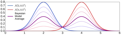
Example 1.6.
If the posterior distribution was approximately equally concentrated on the models and with , that is, two (unimodal) Gaussian distributions with unit variance, then the standard model average is a bimodal non-Gaussian distribution with variance strictly larger than .
Example 1.7.
In the parametric Bayesian model discussed in Example 1.1, the Bayesian model average estimator is the convolution of distributions on :
| (1.10) |
that is, a Gaussian density with mean equal to the posterior mean estimator —see eq. (1.7)— and a covariance matrix that is strictly larger (in the usual order on nonnegative definite symmetric matrices) than that of the predictive posterior law associated with it.
The Bayesian estimators considered Proposition 1.5, eqs. (1.8)-(1.9), share the following characteristic: their values at each point are computed in terms of some posterior average of the values of certain functions evaluated at . This is due to the fact that the corresponding distances/divergences on probability distributions are “vertical” [43]: computing the distance between distributions and involves the integration of vertical displacements between the graphs of their densities across their domain. An undesirable fact about vertical averages is that they are not well suited to incorporate geometric properties into the model space (as illustrated by Example 1.6). More generally, model averages might yield solutions that can be hardly interpretable in terms of the prior and parameters, or even be intractable. This motivates us to explore the use of “horizontal” distances between probability distributions, thus extending the concept of Bayes estimator by making use of the geometric features of the model space. The next section presents the main ideas we will rely on to build such Bayes estimators.
2. Wasserstein distances and Barycenters: a quick review
We shall now introduce objects analogous to those in Proposition 1.5 but suited to Wasserstein distances on the space of probability measures. The following framework is adopted in the sequel:
Assumption 2.1.
The metric space is a separable locally-compact geodesic space endowed with a -finite Borel measure and .
By geodesic we mean that the space is complete and any pair of points admit a mid-point with respect to . Next, we briefly recall some basic elements of optimal transport theory and Wasserstein distances, referring to [45, 46] for general background.
2.1. Optimal transport and the Wasserstein distance
Given two measures over we denote by the set of transport plans or couplings with marginals and , i.e., if and only if , and . Given a real number we define the -Wasserstein space by
The -Wasserstein distance between measures and is given by
| (2.1) |
An optimizer of the right-hand side of eq. (2.1) always exists and is called an optimal transport. The distance turns into a complete metric space. If in eq. (2.1) we assume that , is the Euclidean space, and if is absolutely continuous, then Brenier’s theorem [45, Theorem 2.12(ii)] establishes the uniqueness of a minimizer, and guarantees that it is supported on the graph of the subdifferential of a convex function. The corresponding gradient is thus called an optimal transport map. Explicit formulae for such optimal transport maps do exist in some cases, e.g., for generic one-dimensional distributions and multivariate Gaussians when (see [14]). Contrary to the distances / divergences considered in Proposition 1.5, Wasserstein distances are horizontal [43], in the sense that they involve integrating horizontal displacements between the graphs of probability densities.
Example 2.2.
Example 2.3.
The -Wasserstein distance between Poisson distributions Pois and Pois is , which can be verified from the well-known expression (valid for general one-dimensional distributions ), and the so-called “Poisson-Gamma dual relation”: . When , the optimal coupling between Pois and Pois is obtained taking Pois and binomial with parameters ) conditionally on . Alternatively, one could consider the coupling , where is a Poisson process with intensity 1.
2.2. Wasserstein barycenter
Let us now recall the Wasserstein barycenter, introduced in [1] and further studied in [40, 28, 33], among others. Our definition slightly extends the ones in those works in that the optimization problem is posed in a possibly strict subset of the usual one.
Definition 2.4.
Let . The -Wasserstein risk of is
Given a measurable set , any measure which attains the quantity
with finite value, is called a -Wasserstein barycenter of over .
Notice that in principle we are not assuming to be a model space for , but this will often be the case. When the support of is infinite and , this object is termed -Wasserstein population barycenter of as introduced in [33]; see [10].
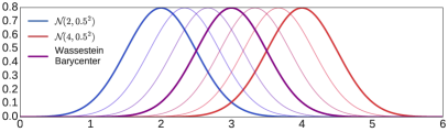
Example 2.5.
Given two univariate Gaussian distributions and , one can verify —using the expression in Example 2.2— that the -Wasserstein barycenter for is given by . This should be compared to Example 1.6. Fig. 1 illustrates the corresponding vertical and a horizontal interpolations between two Gaussian densities with different means and the same variance.
Let us introduce additional notation for the sequel and review then some basic properties of Wasserstein barycenters. Considering with the complete metric as a base Polish metric space, we define in the natural way: is an element of if it is concentrated on a set of measures with finite moments of order , and moreover for some (and then all) it satisfies
We endow with the corresponding Wasserstein distance, which we also denote for simplicity. Also, if is concentrated on measures with finite moments of order which have densities with respect to , then we write and use the notation if, as before, for some .
Remark 2.6.
If has a -Wasserstein barycenter over , then
hence . Moreover, is equivalent to the corresponding model average having a finite -moment, since for any ,
We next state an existence result first established in [33, Theorem 2] for the case . See Appendix B for a simpler, more direct, proof.
Theorem 2.7.
Suppose Assumption 2.1 holds, , and is a weakly closed set. There exists a -Wasserstein barycenter of over if and only if .
Regarding uniqueness, the following general result was proven in [33, Proposition 6] for the case with the Euclidean distance and (observe that, in that situation, the previous result applies):
Lemma 2.8.
Assume and that there exists a set of measures with
and . Then, admits a unique -Wasserstein population barycenter over .
Remark 2.9.
Observe that the model space is not weakly closed. Nevertheless, the existence and uniqueness of a population barycenter over that set can still be guaranteed when , , is the Euclidean distance, is the Lebesgue measure, and
| (2.2) |
This was proven in [28, Theorem 6.2] for compact finite-dimensional manifolds with lower-bounded Ricci curvature (equipped with the volume measure), but one can read-off the (non-compact but flat) Euclidean case from the proof therein, in order to establish the absolute continuity of a barycenter over , in the setting of Lemma 2.8. If then eq. (2.2) can be relaxed to the condition , as shown in [1] or [28, Theorem 5.1].
The following statement, corresponding to [7, Lemma 3.1], provides a useful description of barycenters which generalizes a result proven in [3] when .
Lemma 2.10.
Assume , , Euclidean distance, Lebesgue measure. Let and . There exists a jointly measurable function which is -a.s. equal to the unique optimal transport map from to at . Furthermore, letting be a barycenter of , we have
3. Bayesian Wasserstein barycenter and statistical properties
Building on the Wasserstein distance as a loss function on models, we arrive to the following central object of the article:
Definition 3.1.
Let us consider a prior with model space and data which determines as in eq. (1.2). We define the -Wasserstein Bayes risk of and a Bayes Wasserstein barycenter (BWB) estimator over respectively as follows:
| (3.1) | |||||
| (3.2) |
if the corresponding minimum is finite.
Example 3.2.
In the setting of Example 1.1, the -Wasserstein loss function on Gaussian models (see Example 2.2) induces the usual quadratic loss on the mean parameters: . Thus, in the notation of eq. (1.5), we have
This implies that, for any tuple of data point the BWB corresponds to the Gaussian distribution with mean that is, the posterior mean estimator of the mean parameter. Moreover, in this particular case the barycentric cost or optimal -Wasserstein Bayes risk equals the trace of the covariance of a random vector with law given in eq. (1.6), i.e., . Notice that the covariance of the BWB is strictly smaller than that of the corresponding BMA estimator in eq. (1.10) (in the usual order on symmetric positive semidefinite matrices). This is, in fact, a general property of the BWB as claimed in Proposition 3.9 below.
Example 3.3.
Similarly, in the parametric setting of Example 1.2, the problem of finding BWB estimators can be written in terms of the parametric loss induced by the corresponding -Wasserstein distance on Poisson distributions, computed in Example 2.3. We thus deduce for that the BWB estimator corresponds, in that setting, to the law Pois with the median of the posterior distribution Gamma; for which an explicit expression is not available.
Example 3.4.
Let us assume and that is supported on continuous models over . Let and denote, respectively, the cumulative distribution function and the right-continuous quantile function of such . The coupling , with distributed like and the increasing map , is known to be optimal for the -Wasserstein distance, for any (see [45, Remark 2.19(iv)]). The BWB of the posterior is also independent of and is characterized via its quantile, as follows:
Interestingly enough, the model average of is in turn characterized by its averaged cumulative distribution function: . See Section 5 in the companion paper [7] for details and further discussion on one-dimensional Wasserstein barycenters, in particular, on geometric properties they inherit from the elements of the support of the prior/posterior.
Remark 3.5.
In the sequel, unless otherwise stated, an a.s. statement about is meant to hold almost surely with respect to the marginal law of a data sample of size (sometimes called prior predictive distribution). In particular, for almost every , such statement holds for almost every sample .
Remark 3.6.
We observe that implies for each that
Indeed, for fixed , (we thank an anonymous referee for pointing this out) the following quantity is finite:
| (3.3) |
However, is in general not enough for to hold a.s. for i.i.d. data points sampled from a fixed law , which would be the natural setting to formulate the question of Bayesian consistency (see next subsection). Corollary 3.19 below ensures this fact for suitable given laws , in the framework of Bayesian consistency. In Appendix C we further provide a sufficient condition on the prior (termed integrability after updates) ensuring that for every possible tuple of data points .
The following statement gathers the discussion in Section 2.2 for the case , as well as the main point of Remark 3.6:
Theorem 3.7.
Suppose Assumption 2.1 holds and the model space is weakly closed. Let be a prior with model space and be the corresponding posterior given the data . The following are equivalent:
-
a)
A -Wasserstein barycenter estimator for over exists a.s.
-
b)
a.s.
-
c)
The model average has a.s. a finite -moment.
Moreover, if , a -Wasserstein barycenter estimator over exists a.s. for every .
We thus make in all the sequel the following assumption:
Assumption 3.8.
and there exists a weakly closed model space for .
We will next study some basic statistical properties of the BWB estimator.
3.1. Variance reduction with respect to BMA
In this subsection, we assume that , Lebesgue measure, Euclidean distance and . Let be the unique population barycenter of in that case, and denote by a measurable function equal a.e. to the unique optimal transport map from to . As a consequence of Lemma 2.10 we have the fixed-point property . Thus, for all convex functions , non negative or with at most quadratic growth, we have
where is the Bayesian model average in eq. (1.8). We have used Jensen’s inequality and Fubini’s theorem. This means that the BWB estimator is less spread, or smaller, in the sense of convex-order of probability measures, than the BMA. As a consequence, we have:
Proposition 3.9.
Consider , and let and respectively denote the BMA and the estimators associated with . Then, we have and . In other words, the BWB estimator has less variance than the BMA. Furthermore, with denoting the mean w.r.t. the or , the corresponding covariances satisfy: in the usual order for symmetric positive semidefinite matrices. The inequalities are strict unless is a Dirac mass.
Proof.
Given the previous discussion, the equality of means is obtained by taking and equal to each coordinate of and the inequality of variances by taking . The inequality for the covariances follows by taking for arbitrary .
For the last claim, we just need to make explicit the corresponding equality case of Jensen’s inequality as used in the preceding discussion. Since is strictly convex, the equality of second moments implies that a.e. , that is a.s. constant. This entails that the map does not depend on and that for a.e. , it holds that . The equality case for the covariances is reduced to the previous one considering their traces using also the equality of means. ∎
3.2. Convergence to the true model and Bayesian consistency
A natural question in Bayesian statistics is whether a given predictive posterior estimator is consistent (see [44, 17, 23]). In short, this means the convergence of the predictive posterior law, in some specified sense, towards the true model , as we observe more and more i.i.d. data sampled from . We are specifically interested in the question of whether the BWB estimator converges to the model and, more precisely, on conditions which guarantee that
| (3.4) |
as , where is for each a BWB over a model space . Here and in the sequel, denotes the product law of the infinite sample of i.i.d. data distributed according to . We will see that this question is linked to the notion of consistency (cf. [23, Definition 6.1]) of the prior, introduced next:
Definition 3.10.
The prior is said to be consistent at in the weak topology (resp. -Wasserstein topology) if for each open neighbourhood of in the weak topology of (resp. -Wasserstein topology of ), one has
Remark 3.11.
We notice that in the literature of Bayesian consistency, see e.g. [44, 23], satisfying the above property (in either topology) would be called “strongly consistent” at in allusion to the -a.s. convergences, whereas the term “weakly consistent” would be used when those convergences hold in probability. Since we will be only dealing with the almost sure notion, in order to avoid possible confusions with topological concepts, the adverb “strongly” is omitted throughout when referring to consistency of the prior, while the adverb “weakly” only refers to the weak topology on probability measures.
The celebrated Schwartz theorem [44] provides sufficient conditions for consistency w.r.t. a given topology, see also [23, Chapter 6] for a modern treatment. A key ingredient is the notion of Kullback-Leibler support:
Definition 3.12.
A measure is an element the Kullback-Leibler support of , denoted
if for every , with the reverse Kullback-Leibler entropy defined as if and as otherwise.
Remark 3.13.
The statistical model is interpreted as being “correct” or well specified, if the data distribution is an element of , the support of w.r.t. the weak topology, see [9, 26, 29, 30, 23]. The condition is stronger. Indeed, by the Csiszar-Pinsker inequality and the fact that the dual bounded-Lipschitz distance (metrizing the weak topology in ) is majorized by the total variation distance, one can check that . In particular, one has for any weakly closed model space for . (The reader may consult the mentioned works for the misspecified framework too.)
Remark 3.14.
If , then , the marginal law of one data point in the Bayesian model defined by . Indeed, for any measurable set such that we have This will be useful later.
We recall (see Theorem 6.17 and Example 6.20 in [23]) the following result which concerns the weak topology:
Theorem 3.15.
Assume (only) that is Polish endowed with a -finite Borel measure , that and that . Then, is consistent at in the weak topology.
We now state a general result relating consistency of at in the -Wasserstein topology and the convergence (3.4) (or consistency of the predictive posterior ), with other asymptotic properties of the posterior laws in the Wasserstein setting. Recall that the notation throughout stands for the Wasserstein distance both in and .
Theorem 3.16.
Suppose Assumptions 2.1 and 3.8 hold, that , and that
| (3.5) |
The following are equivalent:
-
a)
, -a.s. as .
-
b)
-a.s. as , we have and the barycentric cost (or optimal Wasserstein Bayes risk or) goes to .
-
c)
is consistent at in the -Wasserstein topology and the moment of the BMA estimator (1.8) converge -a.s. to that of as , i.e. for some (and then all) we have
(3.6) -
d)
is consistent at in the weak topology and for some (and then all) we have
(3.7)
Proof.
By minimality of a barycenter over ,
Thus, for some depending only on ,
| (3.8) | ||||
| (3.9) |
proving that a) b). The converse b) a) follows from
Let us now show that a) c). The convergence implies (by the Portmanteau theorem) that for all closed sets of . Taking with a neighborhood of yields the consistency of at in the -Wasserstein topology. Moreover it implies that for each ,
as . Choosing , we have for any , from where (3.6) follows.
We next prove that c) a). The space being Polish, there is countable basis of open neighborhoods of such that -a.s., for all . Thus, if is any open set such that , for some we have and therefore , -a.s. This implies, by the Portmanteau theorem, that the sequence weakly converges to , -a.s., as probability measures on the metric space . As in the previous (converse) implication, we obtain from (3.6) the convergence of some moments of order of , to the corresponding moment of , -a.s. This plus the weak convergence just established imply that -a.s.
We have thus established that a), b) and c) are equivalent. Notice now that the function
| (3.10) |
is continuous on , since is continuous with polynomial growth of order on . Moreover, , that is, has polynomial growth of order at most on . Therefore, if a) or equivalently c) holds, we have -a.s. that
which is tantamount to (3.7). Moreover if c) holds, consistency of at in the weak topology is obvious. This shows that c) d).
Last, if d) holds, we deduce with Markov’s inequality that, for each rational ,
| (3.11) |
as . This, together with the consistency of at w.r.t. weak topology, is equivalent to having that consistency w.r.t. the Wasserstein topology. Moreover, we have
and so the convergence (3.7) implies the convergence (3.6). This and the previous show that d) implies c), concluding the proof.
∎
Remark 3.17.
The convergence (3.11) for each is exactly what one must add to consistency at of in the weak topology to obtain such consistency in the -Wasserstein topology. However, the latter is only equivalent to the -a.s. weak convergence of to as measures on the metric space as , which is not enough to grant the -a.s. convergence in of to . Similarly, consistency at of in the -Wasserstein topology cannot in general be obtained by adding only the convergence of moments 3.6 to the consistency at of in the weak topology. Of course, if the space is bounded, weak and -Wasserstein topologies on it coincide, and consistency of at in the weak topology implies in that case the convergence (3.7) (since the function in the previous proof is in that case continuous and bounded). Hence, in that case, all the equivalent properties in Theorem 3.16 are satisfied. The same is true if a.e. is supported on a fixed bounded (weakly) closed set (just replace by ).
An immediate consequence of the proof of Theorem 3.16 (cf. the estimate (3.8)) is the following bound, which can be used to obtain quantitative estimates for the average rate of convergence of the BWB, if the posterior and the Wasserstein distance between models are explicit enough:
Corollary 3.18.
Under the assumptions of Theorem 3.16, for some constant we have
The following result gathers sufficient conditions for consistency at of in the -Wasserstein topology and convergence of the BWB.
Corollary 3.19.
Suppose Assumptions 2.1 and 3.8 hold, and moreover that . Then is consistent at in the weak topology and condition (3.5) holds. If moreover either condition (i) or (ii) below hold, then is consistent at in the -Wasserstein topology and , -a.s. as :
-
(i)
the convergence (3.7) holds;
-
(ii)
for some , -a.s. the moments of the BMA estimator are bounded uniformly in .
Proof.
In view of Theorem 3.15, to prove the first claim we just need to prove that (3.5) holds. To that end, let us first check that, whenever , we have If measurable is such that , then for a.e. and every , , one has , from which we get by Remark 3.14, hence . We conclude noting that the set has null - measure, by Remark 3.6.
Given the previous and part d) of Theorem 3.16, the convergence (3.7) immediately implies that is consistent at in the -Wasserstein topology and that -a.s. as . To conclude the proof it is enough to show that the -a.s. uniform boundedness of the moments of the BMA estimator for some , implies, under the given assumptions, that said convergence (3.7) holds. Consider to that end the function defined by (3.10) in the proof of Theorem 3.16. For each we have
The assumption on the moments of the BWA estimators imply that is finite, -a.s., following from applying Jensen’s inequality to the convex function on and the integral w.r.t. defining . Since is arbitrary, it just remains to ensure that -a.s. as (that is, the convergence (3.11) holds). The elementary relations and for all yield the bound
where the first term on the r.h.s. goes -a.s. to as , since is a bounded continuous function and is consistent at in the weak topology. The second term on the r.h.s. is bounded by
For each , this expression can be made arbitrarily small by taking large enough, since and because the uniform boundedness of the moments of the BWA estimators implies their moments are uniformly integrable. We conclude that -a.s. as as desired. ∎
Example 3.20.
Given Gaussian distributions and on , one can check that and hence that in the parametric Bayesian model dealt with in Examples 1.1 and 3.2. Therefore, by Theorem 3.15, in those examples is consistent w.r.t. the weak topology at for any . Moreover, the prior is easily seen to be in , hence Lemma 3.19 ensures that a.s. for all . This fact alternatively follows from the existence of a Wasserstein barycenter for for any data points , verified in this case. To verify consistency of in the -Wasserstein topology at any as well as convergence of the BWB, let us compute and apply directly Theorem 3.16. Denoting by a r.v. with law , we find
with as and
which a.s. goes to as by the Law of Large Numbers, whenever the data consists of an i.i.d. sample from the true model . Notice that the identity found in this case, can be seen as a bias-variance type decomposition for the posterior law on . In this case, one can readily see that .
Example 3.21.
Although the BWB estimator in the Poisson parametric Bayesian model of Example 1.2 is not explicit (see Example 3.3), we can still apply Theorem 3.16 a) to prove that it converges to the true model generating the data. Indeed, if Pois, using the expression for the Wasserstein distance between Poisson laws computed in Example 2.3 we see that
with a r.v. with law Gamma. An elementary computation using the Gamma distribution’s mean and variance shows, in this case, that
which goes to zero a.s. as , whenever the data is an i.i.d. sample from the true model . We deduce with Corollary 3.19 that .
As noticed earlier, consistency of at w.r.t. the -Wasserstein topology is not enough to grant that . But we will see next that this is true under a boundednees condition on the support of . Recall that is said to be bounded in if
A typical example is the finitely parametrized case with compact parameter space and continuous parametrization mapping . More generally, amounts to being supported on a set of models with centered moments bounded by a constant. In particular, and the support of every may be unbounded, and still be bounded. We have
Lemma 3.22.
If is consistent at in the -Wasserstein topology and is bounded in , then as .
Proof.
Let and , then
Since is arbitrary, we only need to check that the second term in the last line goes -a.s. to zero as . By consistency we have a.s. as , and since , we conclude that
∎
Remark 3.23.
consistent at in the weak topology and bounded in is in general not enough to obtain the conclusion of Lemma 3.22. To see this, write
| (3.12) |
where is a fixed small weak neighborhood of (e.g. one can use the bounded Lipschitz distance to build ). As in the proof of Lemma 3.22, the second term in the r.h.s. of (3.12) goes -a.s. to zero as in this case too. However there is no reason why the term should be small. The reason is that for the functional , even if bounded on , there is no reason why should be small (no matter how small may be). Indeed, the statement “ is small if is small” would mean mathematically that the weak and the Wasserstein topologies coincide on locally around , but this is not true in general, even if is bounded111For instance, for and we have that is Wasserstein bounded, and yet weakly but not in Wasserstein topology.. This should not be confused with the fact that, if equiped with the Wasserstein topology and metric is bounded, then on weak and -Wasserstein convergence coincide. Consistency at of in the weak topology, on the other hand, is equivalent to , -a.s. in the weak topology of , when is equipped with the weak topology. This does not imply , -a.s. in the weak topology of , when is equipped with the Wasserstein topology, and hence provides another point of view as to why the l.h.s. of (3.12) does not go to zero without stronger assumptions.
The next result based on Schwartz theorem provides a (rather strong) condition ensuring that the equivalent properties in Theorem 3.16 hold. Unfortunately, we have not been able to prove such a result under more general assumptions.
Theorem 3.24.
Before proving Theorem 3.24 some remarks on its assumptions and proof are in order.
Remark 3.25.
The uniform control assumed on exponential moments implies, by Jensen’s inequality, that By triangle inequality, this in turn implies that is bounded.
Remark 3.26.
The general picture of Bayesian consistency (including the misspecified case) parallels in several aspects Sanov’s large deviations theorem (see e.g. the Bayesian Sanov Theorem in [26, Theorem in 2.1] and references therein), and it similarly relies on exponential controls of (posterior) integrals. The proof of Theorem 3.24 follows the argument of [23, Example 6.20], where Theorem 3.15 above is obtained by combining Schwartz’ theorem ([23, Theorem 6.17]) with Hoeffding’s concentration inequality, to get uniform exponential controls of the posterior mass of complements of weak neighborhoods of , which are defined in terms of bounded random variables. A exponential moment control is what is needed to derive such concentration inequalities for unbounded random variables (e.g. moments), defining neighborhoods in the Wasserstein topology. Notice that finite exponential moments are also required for Sanov’s theorem to hold in the Wasserstein topology [47]. The uniform bound on exponential moments appears however too strong an assumption (it does not hold e.g. in the setting of Example 3.20). The question of relaxing that condition is left for future work.
Remark 3.27.
Proof of Theorem 3.24.
First we show that if is any -neighbourhood of then -a.s. we have . According to Schwartz Theorem in the extended form [23, Theorem 6.17], under the assumption that , it is enough to find for each such a sequence of measurable functions or “tests” such that
-
(1)
, and
-
(2)
First we will construct tests that satisfy Point 1 and Point 2 above, over an appropriate subbase of neighbourhoods , to finally extend those properties to general neighborhoods.
Recall that in iff for all continuous functions on with for some it holds that ; see [46]. Given such and we define the open sets
which form a sub-base for the -Wasserstein neighborhood system at the distribution . We can assume that by otherwise considering instead. Given a neighborhood of as above, we define the test functions
By the law of large numbers, , so Point 1 is verified. Point 2 is trivial if , so we assume from now on that . Thanks to the exponential moments control assumed on , for a.e. the random variable with has a moment-generating function which is finite for all , namely
We thus have the bounds
for all . Therefore, we may apply Bernstein’s inequality in the form of [36, Corollary 2.10] to the random variables under the measure on , obtaining for any that
with , , and . Going back to the tests and using the definition of we deduce that
Thanks to the uniform control of exponential moments on the support, we conclude as desired that
Now, a general neighborhood contains a finite intersection of, say, elements of the sub-base, i.e. , so
Therefore we can conclude as in the sub-base case that Point 2 is verified. All in all, we have established that is -Wasserstein consistent at . Thanks to Lemma 3.22 and the boundedness of (see Remark 3.25) the last two claims are immediate. ∎
4. BWB calculation through descent algorithms in Wasserstein space
In this section we review some of the available methods to compute Wasserstein barycenters, and then explain how they can be used to calculate the BWB estimator. We will first survey the method proposed by Álvarez-Esteban, Barrio, Cuesta-Albertos and Matrán in [3, Theorem 3.6] and by Zemel and Panaretos in [48, Theorem 3, Corollary 2], applicable in the setting where the probability distribution on the model space has finite support. This method is interpreted in [48] as a gradient descent in the Wasserstein space. We will then discuss the main aspects of the stochastic gradient descent in Wasserstein space (SGDW), introduced in our companion paper [7], building also upon the gradient descent idea. The latter method allows moreover the computation of population barycenters for a distribution on the model space, using a streaming of random probability distributions sampled from it. In particular, we will recall the conditions established in [7] which ensure its convergence. The reader is referred to [41, 16, 34, 18] for alternative approaches to computing Wasserstein barycenters.
The two discussed methods can be easily implemented when explicit analytical expressions for optimal transport maps between distributions in the model space are available (see [7] or Section 5 for some examples). Moreover, in that case these methods can easily be coupled with sampling procedures (MCMC or others) for the posterior distribution in order to compute the BWB. We will see that the computation of the BWB through the SGDW has several advantageous features. In particular, when expressions for optimal transport maps are known, it can be done at nearly the same cost as the posterior sampling.
From now on we specialize Assumption 2.1, and make the following set of assumptions:
Assumption 4.1.
, , Euclidean metric, Lebesgue measure. Furthermore, and there is a model space for which is weakly closed.
The following concept will be central in the “gradient-type” algorithms we consider:
Definition 4.2.
We say that is a Karcher mean of if
Remark 4.3.
It is known that any 2-Wasserstein barycenter is a Karcher mean (c.f. [48]). However, the class of Karcher means is in general a strictly larger one, see [3]. For conditions ensuring uniqueness of Karcher means, see [48, 38] for the case when the support of is finite and [10] for the case of an infinite support. In one dimension, the uniqueness of Karcher means holds without further assumptions. See [7] for a deeper discussion.
4.1. Gradient descent on Wasserstein space
Consider finitely supported: for some , , we have
Following [3] and [48], we define an operator over by
| (4.1) |
Starting from one can then define the sequence
| (4.2) |
The next result proven in [3, Theorem 3.6] and independently in [48, Theorem 3, Corollary 2], establishes the convergence of the above sequence to a fixed-point of , which is nothing other than a Karcher mean for :
Proposition 4.4.
The sequence in eq. (4.2) is tight and every weakly convergent subsequence of converges in to an absolutely continuous measure in which is a Karcher mean of . If some has a bounded density, and if there exists a unique Karcher mean , then is the Wasserstein barycenter of and .
Panaretos and Zemel [48, Theorem 1] discovered that the sequence (4.2) can indeed be interpreted as a gradient descent (GD) scheme with respect to the Riemannian-like structure of the Wasserstein space . In fact, the functional on given by
has a Frechet derivative at each point , given by
where is the identity map in . This means that for each such , one has
| (4.3) |
when goes to zero, by virtue of [5, Corollary 10.2.7]. It follows from Brenier’s theorem [45, Theorem 2.12(ii)] that is a fixed point of defined in eq. (4.1) if and only if . The gradient descent sequence in Wasserstein space (GDW) with step starting from is defined by (c.f. [48])
and it coincides with the sequence in eq. (4.2) if . These ideas serve as inspiration for the stochastic gradient descent iteration in the next part.
4.2. Stochastic gradient descent for population barycenters
We recall next the stochastic gradient descent sequence introduced in the companion paper [7], where the reader is referred to for details. Additionally to the assumptions in the previous part, we will also make use of an extra one introduced in [7]:
Assumption 4.5.
has a -compact model space . Moreover this set is geodesically convex: for every and , , with the identity operator.
In particular, under these assumptions, for each and a.e. , there is a unique optimal transport map from to and, by [33, Proposition 6], the 2-Wasserstein population barycenter is unique. We notice that, although strong at first sight, assumption 4.5 can be guaranteed in suitable parametric situations (e.g., Gaussian, or even the location scatter setting recalled in Section 5.1), or under moment and density constraints on the measures in (e.g., under uniform bounds on their moments of order and their Boltzmann entropy, which are geodesically convex functionals, see [5]).
Definition 4.6.
Let , , and for . We define the stochastic gradient descent in Wasserstein space sequence (SGDW) by
| (4.4) |
The sequence is a.s. well-defined, as one can show by induction that a.s. thanks to Assumption 4.5. The rationale for definition 4.4 is similar to that of Section 4.1, though now we wish to emphasize the population case: If we call now
| (4.5) |
the functional minimized by a 2-Wasserstein barycenter, then we (formally at least) expect
| (4.6) |
Hence, with , is an unbiased estimator of . This immediately suggests the stochastic descent sequence (4.4) introduced in [7], drawing inspiration from the classic SGD ideas [42].
Clearly is a Karcher mean for iff . Just like for the GD sequence, the SGD sequence is typically expected to converge to stationary points, or Karcher means in the present setting, rather than to minimisers. Next theorem provides sufficient conditions for the SGDW sequence to a.s. converge to a Wasserstein barycenter, and is the main result of [7]. The following assumption on the steps , standard in the framework of SGD methods, is needed:
| (4.7) |
4.3. Batch stochastic gradient descent on Wasserstein space
We briefly recall how the variance of the SGDW sequence can be reduced by using batches:
Definition 4.8.
Let , , and for and . The batch stochastic gradient descent (BSGD) sequence is given by
| (4.8) |
The following two results, extracted from [7], justify the above definition: The first result states that this sequence is still converging, while the second one states that batches help reducing noise:
Proposition 4.9.
Proposition 4.10.
The batch estimator for of batch size , given by , has integrated variance
i.e. decreasing linearly in the batch size.
4.4. Computation of the BWB
It is immediate to deduce a simple methodology based on the SGDW algorithm, to compute the BWB estimator for general (finitely or infinitely supported) posterior laws .
We make the practical assumption that we are capable of generating independent models from the posteriors (in the parametric setting, this can be done through efficient Markov Chain Monte Carlo (MCMC) techniques [6, 25, 11] or transport sampling procedures [20, 39, 27, 35]). On the theoretical side, we assume conditions 4.1 and 4.5 are satisfied by , the prior law on models, implying the posterior a.s. satisfies those conditions for all too.
The proposed method can be sketched as follows:
-
(1)
Given a prior on models and data , sample and set .
-
(2)
Sample independent from
-
(3)
Set
-
(4)
Increase by and go to (2).
The algorithm can be run until large enough such that the squared Wasserstein distance
between and is repeatedly smaller than some given positive threshold.
Moreover, under the assumptions of Theorem 3.24, is consistent in the -topology at the law of the data and then, for some (random) large enough and given one has where is the . Notice that, besides the sequential generation of a finite i.i.d. sequence , at each step one only needs to compose a new transport map with the transport map pushing forward to , cumulatively constructed in the previous iterations. If an expression for each map is available, this can easily be done (and stored), specifying (only) the values of the lastly computed map on a pre-fixed grid.
The batch version SGWD can be implemented in a similar way to compute the BWB estimator.
Remark 4.11.
An alternative, natural approach would be to sample, for given a fixed number of realizations , , and compute, using the GDW algorithm, the Wasserstein barycenter of the (finitely supported) empirical measure
or -Wasserstein empirical barycenter of (see [10]). Indeed, by Varadarajan’s theorem, conditionally on , a.s. converges weakly as to , and in the metric as soon as . Since under our assumptions a.s. has a unique -Wasserstein barycenter and, by [33, Theorem 3], converges with respect to a.s. as to it, we also get through this approach that
for some (random) large enough . The clear disadvantage of this method is computational: besides generating samples of , we need to additionally run a possibly large number of GDW steps to approximate , and we need to evaluate at each step new transport maps (instead of one, for the SGDW). Moreover, if additional new samples from become available, we need to run the whole scheme again to take advantage of this new information. On the contrary, the online nature of the SGDW method allows one to refine the already computed estimator by only performing new steps of the algorithm.
5. Numerical experiments
Before presenting the experimental validation of the proposed methods we give a brief presentation of the scatter-location family of distributions. Our experiments consider this family because the optimal transport maps between two laws in the scatter-location family can be described explicitly. This property facilitates the numerical computation/approximation of barycenters, as the various iterative algorithms described so far take a more amenable form. See [7] for further examples.
5.1. Location-Scatter family
We follow the setting of [4]: Given a fixed distribution , referred to as generator, the associated location-scatter family is given by
where is the set of symmetric positive definite matrices of size . Without loss of generality we can assume that has zero mean and identity covariance. Note that is the multivariate normal family if is the standard multivariate normal distribution.
The optimal map between two members and of is explicit, given by where . This family of optimal maps contains the identity and is closed under convex combination.
If is supported on , then its -Wasserstein barycenter belongs to . In fact, call its mean and its covariance matrix . Since the optimal map from to is , where , and we know that , -almost surely, then we must have that , since clearly , and as a consequence .
A stochastic gradient descent iteration, starting from a distribution , sampling some , and with step , produces the measure . If has a multivariate distribution , then has distribution with mean and covariance . We have that with . Then has distribution
with mean and covariance
The batch stochastic gradient descent iteration is characterized by
5.2. Experiment
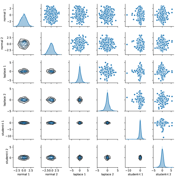
We considered a model within a location-scatter family (LS), with generator on with independent coordinates, as follows:
-
•
coordinates 1 to 5 are standard Normal distributions
-
•
coordinates 6 to 10 are standard Laplace distributions, and
-
•
coordinates 11 to 15 are standard Student’s -distributions ( degrees of freedom).
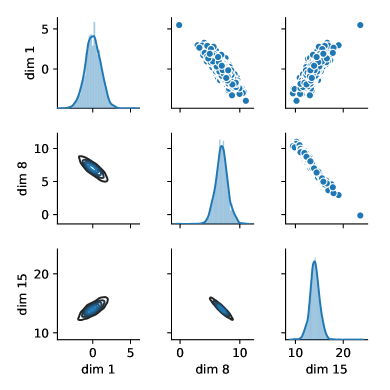
Fig. 2 shows samples (uni- and bi-variate marginals) from coordinates of .
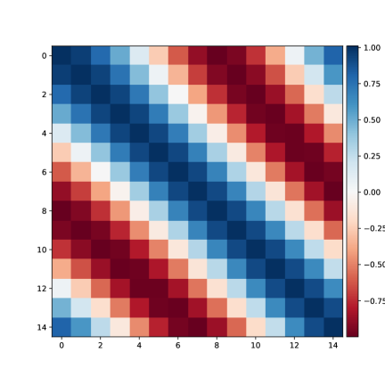
In this LS family, we chose the true model with location vector defined as for , and scatter matrix with for 222We chose for because this defines a non-uniform grid over ., with the covariance (kernel) function . Given the parameters and , the so constructed covariance matrix will be denoted . We chose the parameters , and for . Thus, under the true model the coordinates can be negatively/positively correlated and there is also a coordinate-independent noise component due to the Kronecker delta . Fig. 3 shows the covariance matrix and three coordinates of the true model .
The model prior is the push-forward induced by a prior over the mean vector and the parameters of the covariance , chosen independently according to :
| (5.1) |
where is a exponential density with rate . Given samples from the true model (also referred to as observations or data points), samples are produced from the posterior measure using Markov chain Monte Carlo (MCMC).
The numerical analysis presented in what follows focuses on the behavior of the BWB as a function of both the number of samples and the number of data points .
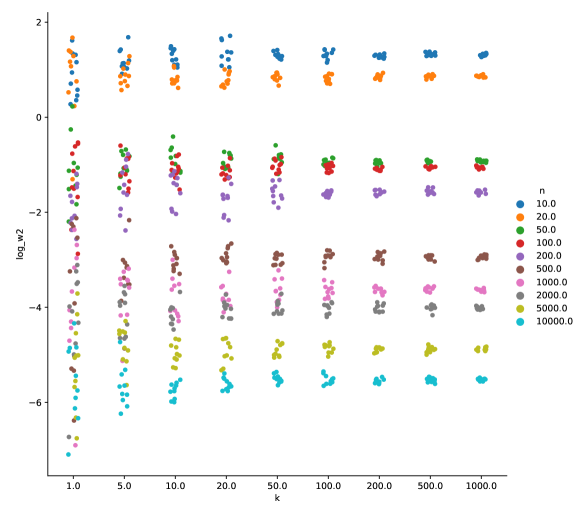
Numerical consistency of the empirical posterior
We first validate the empirical measure as a consistent sample version of the true posterior under the distance, that is, we check that for large . We estimate 10 times for each combination of the (number of) observations and samples in the following sets
-
•
-
•
Fig. 4 shows the 10 estimates of for different values of (in the -axis) and of (color coded). Notice how the estimates become more concentrated for larger and that the Wasserstein distance between the empirical measure and the true model decreases for larger . Additionally, Table 1 shows that the standard deviation of the 10 estimates of decreases as either or increases.
| n \ k | 1 | 5 | 10 | 20 | 50 | 100 | 200 | 500 | 1000 |
|---|---|---|---|---|---|---|---|---|---|
| 10 | 1.2506 | 0.8681 | 0.5880 | 0.9690 | 0.2354 | 0.3440 | 0.1253 | 0.1330 | 0.0972 |
| 20 | 1.5168 | 0.5691 | 0.3524 | 0.3182 | 0.1850 | 0.1841 | 0.1049 | 0.0811 | 0.0509 |
| 50 | 0.3479 | 0.0948 | 0.1275 | 0.0572 | 0.0623 | 0.0229 | 0.0157 | 0.0085 | 0.0092 |
| 100 | 0.2003 | 0.1092 | 0.0712 | 0.0469 | 0.0431 | 0.0254 | 0.0087 | 0.0079 | 0.0084 |
| 200 | 0.0749 | 0.1249 | 0.0717 | 0.0533 | 0.0393 | 0.0101 | 0.0092 | 0.0109 | 0.0072 |
| 500 | 0.0478 | 0.0285 | 0.0093 | 0.0086 | 0.0053 | 0.0056 | 0.0045 | 0.0023 | 0.0022 |
| 1000 | 0.0299 | 0.0113 | 0.0113 | 0.0064 | 0.0067 | 0.0036 | 0.0016 | 0.0012 | 0.0007 |
| 2000 | 0.0145 | 0.0071 | 0.0040 | 0.0031 | 0.0027 | 0.0019 | 0.0014 | 0.0011 | 0.0006 |
| 5000 | 0.0072 | 0.0031 | 0.0015 | 0.0018 | 0.0010 | 0.0007 | 0.0004 | 0.0005 | 0.0002 |
| 10000 | 0.0038 | 0.0020 | 0.0005 | 0.0005 | 0.0004 | 0.0004 | 0.0002 | 0.0002 | 0.0001 |
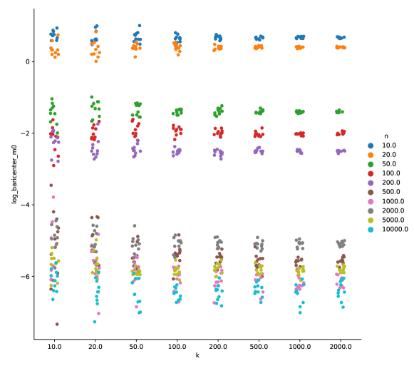
Wasserstein distance between the empirical barycenter and the true model
For each empirical posterior , we computed the empirical Wasserstein barycenter as suggested in Remark 4.11. Thus, we used the iterative GDW procedure in eq. (4.2), namely the (deterministic) gradient descent method, and repeated this calculation 10 times. As a stopping criterion for gradient descent, we considered the relative variation of the cost; the computation was terminated when this cost fell below . Fig. 5 shows the distances between the so computed barycenters and the true model, while Table 2 shows the average distance for each pair (). Notice that, in general, both the average and standard deviation of the barycenters decrease as either or increases, yet for large values (e.g., ) numerical issues appear.
| n / k | 10 | 20 | 50 | 100 | 200 | 500 | 1000 | 2000 |
|---|---|---|---|---|---|---|---|---|
| 10 | 2.1294 | 2.0139 | 2.0384 | 1.9396 | 1.9608 | 1.9411 | 1.9699 | 1.9548 |
| 20 | 1.4382 | 1.4498 | 1.4826 | 1.4973 | 1.4785 | 1.4953 | 1.4955 | 1.4914 |
| 50 | 0.2455 | 0.2759 | 0.2639 | 0.2468 | 0.2499 | 0.2483 | 0.2443 | 0.2454 |
| 100 | 0.1211 | 0.1387 | 0.1509 | 0.1458 | 0.1379 | 0.1328 | 0.1318 | 0.1349 |
| 200 | 0.1116 | 0.0922 | 0.0859 | 0.0817 | 0.0777 | 0.0824 | 0.0820 | 0.0819 |
| 500 | 0.0094 | 0.0077 | 0.0043 | 0.0047 | 0.0041 | 0.0038 | 0.0037 | 0.0039 |
| 1000 | 0.0068 | 0.0039 | 0.0031 | 0.0025 | 0.0023 | 0.0022 | 0.0021 | 0.0021 |
| 2000 | 0.0072 | 0.0066 | 0.0063 | 0.0062 | 0.0063 | 0.0060 | 0.0062 | 0.0062 |
| 5000 | 0.0037 | 0.0037 | 0.0028 | 0.0029 | 0.0031 | 0.0031 | 0.0028 | 0.0030 |
| 10000 | 0.0023 | 0.0017 | 0.0017 | 0.0015 | 0.0016 | 0.0017 | 0.0016 | 0.0017 |
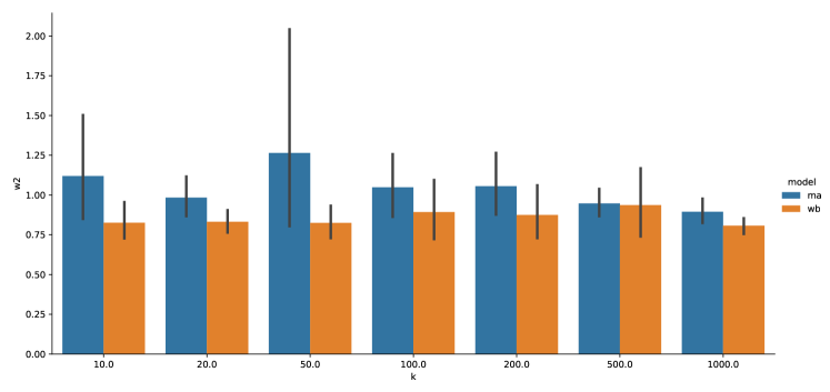
Distance between the empirical barycenter and the Bayesian model average
We then compared the empirical Wasserstein barycenters to the standard Bayesian model averages, denoted here , in terms of their distance to the true model , for observations. To that end, we estimated the distances via empirical approximations with samples for each model based on [21]. We simulated this procedure 10 times for . Fig. 6 shows the sample average and variance of the distances of the Wasserstein barycenters and Bayesian model averages. The empirical barycenter is seen to be closer to the true model than the model average, regardless of the number of MCMC samples .
Computation of the Wasserstein barycenter with batch-SGDW
Lastly, we compared the empirical barycenters to the barycenter obtained by the batch SGDW method in eq. (4.8) with different batch sizes. Here, we shall denote the latter by with the number of observations, the steps of the algorithm, and the batch size. Fig. 7 shows the evolution of the distance between the stochastic gradient descent sequences and the true model for observations and batches of sizes , with step-size for . Notice from Fig. 7 that the larger the batch, the more concentrated the trajectories of become. Additionally, Table 3 summarizes the means of the distance to the true model , using the sequences after against the empirical estimator using all the simulations with . Finally, Table 4 shows the standard deviation of the distance to the true model , which can be seen to decrease as the batch size grows. Critically, we observe that for batch sizes the stochastic estimation was better than its empirical counterpart, i.e., it had smaller variance with similar (or even smaller) bias. This is noteworthy given the fact that computing our Wasserstein barycenter estimator via the batch stochastic gradient descent method is computationally less demanding than computing it via the empirical method.
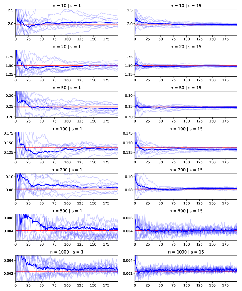
| n / s | 1 | 2 | 5 | 10 | 15 | 20 | empirical |
|---|---|---|---|---|---|---|---|
| 10 | 2.0421 | 2.0091 | 1.9549 | 1.9721 | 1.9732 | 1.9712 | 1.9532 |
| 20 | 1.4819 | 1.4868 | 1.5100 | 1.4852 | 1.4840 | 1.4891 | 1.4916 |
| 50 | 0.2406 | 0.2512 | 0.2465 | 0.2427 | 0.2444 | 0.2460 | 0.2469 |
| 100 | 0.1340 | 0.1392 | 0.1340 | 0.1349 | 0.1334 | 0.1338 | 0.1366 |
| 200 | 0.0843 | 0.0811 | 0.0819 | 0.0807 | 0.0820 | 0.0819 | 0.0811 |
| 500 | 0.0044 | 0.0042 | 0.0039 | 0.0039 | 0.0041 | 0.0040 | 0.0041 |
| n / s | 1 | 2 | 5 | 10 | 15 | 20 | empirical |
|---|---|---|---|---|---|---|---|
| 10 | 0.1836 | 0.1071 | 0.0526 | 0.0474 | 0.0397 | 0.0232 | 0.0916 |
| 20 | 0.0751 | 0.0565 | 0.0553 | 0.0189 | 0.0253 | 0.0186 | 0.0790 |
| 50 | 0.0210 | 0.0174 | 0.0072 | 0.0084 | 0.0050 | 0.0039 | 0.0138 |
| 100 | 0.0102 | 0.0076 | 0.0049 | 0.0048 | 0.0035 | 0.0023 | 0.0112 |
| 200 | 0.0074 | 0.0045 | 0.0021 | 0.0035 | 0.0013 | 0.0017 | 0.0047 |
| 500 | 0.0016 | 0.0007 | 0.0005 | 0.0004 | 0.0004 | 0.0004 | 0.0009 |
| 1000 | 0.0005 | 0.0006 | 0.0004 | 0.0004 | 0.0003 | 0.0003 | 0.0005 |
Conclusion
Based on this illustrative numerical example, we can conclude:
-
•
the empirical posterior constructed using MCMC is consistent under the distance and therefore it can be relied upon to compute Wasserstein barycenters,
-
•
the empirical Wasserstein barycenter estimator tends to converge faster (and with lower variance) to the true model than the empirical Bayesian model average,
-
•
computing the population Wasserstein barycenter estimator via batch stochastic gradient descent is promising as an alternative to computing the empirical barycenter (i.e., to applying the deterministic gradient descent method to a finitely-sampled posterior).
Acknowledgments
We would like to thank two anonymous referees for suggesting us some of the parametric examples we have analyzed, and for their valuable questions and comments, which allowed us to clarify the presentation of the paper and refine our results. This work was partially funded by the ANID-Chile grants: Fondecyt-Regular 1201948(JF) and 1210606 (FT); Center for Mathematical Modeling ACE210010 and FB210005 (JF, FT); and Advanced Center for Electrical and Electronic Engineering FB0008 (FT).
References
- [1] Martial Agueh and Guillaume Carlier. Barycenters in the Wasserstein space. SIAM Journal on Mathematical Analysis, 43(2):904–924, 2011.
- [2] Jason Alschuler and Enricm Boix-Adsera. Wasserstein barycenters are NP-hard to compute. arXiv preprint arXiv:2101.01100, 2021.
- [3] Pedro C Álvarez-Esteban, Eustasio del Barrio, Juan A Cuesta-Albertos, and Carlos Matrán. A fixed-point approach to barycenters in Wasserstein space. Journal of Mathematical Analysis and Applications, 441(2):744–762, 2016.
- [4] Pedro C Álvarez-Esteban, Eustasio del Barrio, Juan A Cuesta-Albertos, and Carlos Matrán. Wide consensus aggregation in the Wasserstein space. application to location-scatter families. Bernoulli, 24(4A):3147–3179, 2018.
- [5] Luigi Ambrosio, Nicola Gigli, and Giuseppe Savaré. Gradient flows in metric spaces and in the space of probability measures. Lectures in Mathematics ETH Zürich. Birkhäuser Verlag, Basel, second edition, 2008.
- [6] Christophe Andrieu, Nando De Freitas, Arnaud Doucet, and Michael I Jordan. An introduction to MCMC for machine learning. Machine learning, 50(1):5–43, 2003.
- [7] J. Backhoff-Veraguas, J. Fontbona, G. Rios, and F. Tobar. Stochastic gradient descent in Wasserstein space. arXiv preprint arXiv:2201.04232, 2022.
- [8] James O Berger. Statistical decision theory and Bayesian analysis. Springer Science & Business Media, 2013.
- [9] Robert H Berk et al. Limiting behavior of posterior distributions when the model is incorrect. The Annals of Mathematical Statistics, 37(1):51–58, 1966.
- [10] Jérémie Bigot and Thierry Klein. Characterization of barycenters in the Wasserstein space by averaging optimal transport maps. ESAIM: Probability and Statistics, 22:35–57, 2018.
- [11] Steve Brooks, Andrew Gelman, Galin Jones, and Xiao-Li Meng. Handbook of markov chain monte carlo. CRC press, 2011.
- [12] Elsa Cazelles, Felipe Tobar, and Joaquin Fontbona. A novel notion of barycenter for probability distributions based on optimal weak mass transport. 2021 Conference on Neural Information Processing Systems NeurIPS, arXiv preprint arXiv:2102.13380, 2021.
- [13] Sinho Chewi, Tyler Maunu, Philippe Rigollet, and Austin J Stromme. Gradient descent algorithms for Bures-Wasserstein barycenters. In Conference on Learning Theory, pages 1276–1304. PMLR, 2020.
- [14] Juan Cuesta-Albertos, L Ruschendorf, and Araceli Tuero-Diaz. Optimal coupling of multivariate distributions and stochastic processes. Journal of Multivariate Analysis, 46(2):335–361, 1993.
- [15] Marco Cuturi and Arnaud Doucet. Fast computation of Wasserstein barycenters. In International Conference on Machine Learning, pages 685–693, 2014.
- [16] Marco Cuturi and Gabriel Peyré. A smoothed dual approach for variational Wasserstein problems. SIAM Journal on Imaging Sciences, 9(1):320–343, 2016.
- [17] Persi Diaconis and David Freedman. On the consistency of Bayes estimates. The Annals of Statistics, pages 1–26, 1986.
- [18] Pierre Dognin, Igor Melnyk, Youssef Mroueh, Jerret Ross, Cicero Dos Santos, and Tom Sercu. Wasserstein barycenter model ensembling. arXiv preprint arXiv:1902.04999, 2019.
- [19] D. C. Dowson and B. V. Landau. The Fréchet distance between multivariate normal distributions. J. Multivariate Anal., 12(3):450–455, 1982.
- [20] Tarek A El Moselhy and Youssef M Marzouk. Bayesian inference with optimal maps. Journal of Computational Physics, 231(23):7815–7850, 2012.
- [21] Rémi Flamary and Nicolas Courty. POT Python Optimal Transport library, 2017.
- [22] Maurice Fréchet. Les éléments aléatoires de nature quelconque dans un espace distancié. In Annales de l’institut Henri Poincaré, volume 10, pages 215–310, 1948.
- [23] Subhashis Ghosal and Aad van der Vaart. Fundamentals of nonparametric Bayesian inference, volume 44. Cambridge University Press, 2017.
- [24] Clark R. Givens and Rae Michael Shortt. A class of Wasserstein metrics for probability distributions. Michigan Math. J., 31(2):231–240, 1984.
- [25] Jonathan Goodman and Jonathan Weare. Ensemble samplers with affine invariance. Communications in applied mathematics and computational science, 5(1):65–80, 2010.
- [26] Marian Grendár and George Judge. Asymptotic equivalence of empirical likelihood and Bayesian map. Ann. Statist., 37(5A):2445–2457, 2009.
- [27] Sanggyun Kim, Diego Mesa, Rui Ma, and Todd P Coleman. Tractable fully Bayesian inference via convex optimization and optimal transport theory. arXiv preprint arXiv:1509.08582, 2015.
- [28] Young-Heon Kim and Brendan Pass. Wasserstein barycenters over Riemannian manifolds. Advances in Mathematics, 307:640–683, 2017.
- [29] Bastiaan Jan Korneel Kleijn. Bayesian asymptotics under misspecification. PhD thesis, Vrije Universiteit Amsterdam, 2004.
- [30] Bastiaan Jan Korneel Kleijn and Adrianus Willem Van der Vaart. The Bernstein-von-Mises theorem under misspecification. Electronic Journal of Statistics, 6:354–381, 2012.
- [31] Alexander Korotin, Vage Egiazarian, Li Lingxiao, and Evgeny Burnaev. Wasserstein iterative networks for barycenter estimation. arXiv preprint arXiv:2201.12245, 2022.
- [32] Julien Lacombe, Julie Digne, Nicolas Courty, and Nicolas Bonneel. Learning to generate Wasserstein barycenters. arXiv preprint arXiv:2102.12178, 2021.
- [33] Thibaut Le Gouic and Jean-Michel Loubes. Existence and consistency of Wasserstein barycenters. Probability Theory and Related Fields, 168(3-4):901–917, 2017.
- [34] Anton Mallasto, Augusto Gerolin, and Hà Quang Minh. Entropy-regularized 2-Wasserstein distance between gaussian measures. Information Geometry, pages 1–35, 2021.
- [35] Youssef Marzouk, Tarek Moselhy, Matthew Parno, and Alessio Spantini. Sampling via measure transport: An introduction. Handbook of uncertainty quantification, pages 1–41, 2016.
- [36] Pascal Massart. Concentration inequalities and model selection. Springer, 2007.
- [37] Kevin P Murphy. Machine learning: a probabilistic perspective. The MIT Press, Cambridge, MA, 2012.
- [38] Victor M. Panaretos and Yoav Zemel. An invitation to statistics in Wasserstein space. SpringerBriefs in Probability and Mathematical Statistics. Springer, Cham, [2020] ©2020.
- [39] Matthew Parno. Transport maps for accelerated Bayesian computation. PhD thesis, Massachusetts Institute of Technology, 2015.
- [40] Brendan Pass. Optimal transportation with infinitely many marginals. Journal of Functional Analysis, 264(4):947–963, 2013.
- [41] Gabriel Peyré and Marco Cuturi. Computational optimal transport: With applications to data science. Foundations and Trends® in Machine Learning, 11(5-6):355–607, 2019.
- [42] Herbert Robbins and Sutton Monro. A stochastic approximation method. The Annals of Mathematical Statistics, pages 400–407, 1951.
- [43] Filippo Santambrogio. Optimal transport for applied mathematicians. Birkäuser, NY, pages 99–102, 2015.
- [44] Lorraine Schwartz. On Bayes procedures. Zeitschrift für Wahrscheinlichkeitstheorie und verwandte Gebiete, 4(1):10–26, 1965.
- [45] Cédric Villani. Topics in optimal transportation, volume 58 of Graduate Studies in Mathematics. American Mathematical Society, Providence, RI, 2003.
- [46] Cédric Villani. Optimal transport. Old and new, volume 338 of Grundlehren der mathematischen Wissenschaften [Fundamental Principles of Mathematical Sciences]. Springer-Verlag, Berlin, 2009.
- [47] Ran Wang, Xinyu Wang, and Liming Wu. Sanov’s theorem in the Wasserstein distance: a necessary and sufficient condition. Statistics & Probability Letters, 80(5-6):505–512, 2010.
- [48] Y. Zemel and V. Panaretos. Fréchet means and Procrustes analysis in Wasserstein space. Bernoulli, 25(2):932–976, 2019.
Appendix A Bayes estimators as generalized model averages
We prove here Proposition 1.5. For notational simplicity we omit the subscripts of estimators and normalizing constants.
i) Squared -distance: By Fubini’s theorem, minimizing in this case amounts to minimize
over the set of densities. But the optimal value cannot be better than if we minimize pointwise the term inside the curly brackets, obtaining the candidate
As this pointwise minimizer is already a probability density, we conclude.
ii) Squared Hellinger distance: Writing
we see that optimizing the asociated Bayes risk amounts to maximizing over the concave functional with for and , under the constraint . Notice by the Cauchy-Schwarz inequality that this functional is finite if (and only if) , -a.e. Hence, introducing a real Lagrange multiplier for the constraint, we need to find a critical point of the concave functional
which must thus be a maximum. Again, as in i), we cannot do better in this case than if we maximize for each the concave functional over . Finding for each the critical point in terms of and integrating then w.r.t. to get rid of , we find the extremum of is attained when equals the Bayesian square model average:
iii) Forward Kullback-Leibler divergence: the loss function is now
and so the associated Bayes risk can be written as
Introducing the Boltzmann entropy of and adjusting the constant we get that
so the optimizer of is the Bayesian model average.
iv) Reverse Kullback-Leibler divergence: since we have
Denote by the normalization constant so that . Then,
Therefore, the extremum of is attained when the last expression vanishes, in other words when is the Bayesian exponential model average given by
Appendix B Wasserstein barycenters
Proof of Theorem 2.7.
Assume . Then is finite. Now, let be such that
For large enough we have
by convexity of optimal transport costs. From this we derive that (for every )
By Markov inequality this shows, for each , that there is large enough such that . As explained in [33], the assumptions on imply that is compact (Hopf-Rinow theorem), and so we deduce the tightness of . By Prokhorov theorem, up to selection of a subsequence, there exists which is its weak limit. By Fatou’s lemma:
hence is a Wasserstein barycenter. For the converse implication, see Remark 2.6. ∎
Appendix C A condition for existence of barycenters of Bayesian posteriors
We last provide a general condition on the prior ensuring that, for given ,
Definition C.1.
We say that is integrable after updates if it satisfies the conditions
-
(1)
For all :
-
(2)
For some and :
Remark C.2.
Condition (2) above can be intuitively denoted as . Of course, one has .
Remark C.3.
If has finite support, then Conditions (1) and (2) are satisfied. On the other hand, if is supported on a scatter-location family (see Section 5.1) containing one element with a bounded density and a finite -moment, then Conditions (1) and (2) are fulfilled if for example is tight. Conditions (1) and (2) are also satisfied in Example 3.2.
Lemma C.4.
Suppose that is integrable after updates. Then, for each , the measure
is also integrable after updates.
Proof.
We verify Property (1) first. Let and given. Then
with conjugate Hölder exponents. This is finite since fulfils Property (1).
We now establish Property (2). Let . Then
The first term in the r.h.s. is finite by Property (1). The second term in the r.h.s. is finite by Property (2), if we take small enough and close enough to . We conclude. ∎
Lemma C.5.
Suppose that is integrable after updates. Then for all and , the posterior is also integrable after updates.
Proof.
By Lemma C.4, we obtain that is integrable after updates. By induction, suppose has this property. Then as
we likewise conclude that is integrable after updates. ∎