On QoS-Compliant Telehaptic Communication over Shared Networks

Abstract

The development of communication protocols for teleoperation with force feedback (generally known as telehaptics) has gained widespread interest over the past decade. Several protocols have been proposed for performing telehaptic interaction over shared networks. However, a comprehensive analysis of the impact of network cross-traffic on telehaptic streams, and the feasibility of Quality of Service (QoS) compliance is lacking in the literature. In this paper, we seek to fill this gap. Specifically, we explore the QoS experienced by two classes of telehaptic protocols on shared networks — Constant Bitrate (CBR) protocols and adaptive sampling based protocols, accounting for CBR as well as TCP cross-traffic. Our treatment of CBR-based telehaptic protocols is based on a micro-analysis of the interplay between TCP and CBR flows on a shared bottleneck link, which is broadly applicable for performance evaluation of CBR-based media streaming applications. Based on our analytical characterization of telehaptic QoS, and via extensive simulations and real network experiments, we formulate a set of sufficient conditions for telehaptic QoS-compliance. These conditions provide guidelines for designers of telehaptic protocols, and for network administrators to configure their networks for guaranteeing QoS-compliant telehaptic communication.

A preliminary version of this article was presented at IEEE International Symposium on Haptic Audio-Visual Environments and Games (HAVE), 2017.
Authors’ address: V. Gokhale, J. Nair and S. Chaudhuri, Department of Electrical Engineering, Indian Institute of Technology Bombay, Mumbai 400076, India; emails: {vineet, jayakrishnan.nair, sc}@ee.iitb.ac.in; V. Gokhale and J. Fesl, Institute of Applied Informatics, University of South Bohemia, České Budějovice 37005, Czech Republic; emails: {vgokhale, jfesl}@prf.jcu.cz.

1 INTRODUCTION

The past two decades have witnessed rapid advancements in the science of exploration and manipulation of remote objects with the augmentation of force feedback – a field generally referred to as telehaptics. The primary aim of telehaptics is to provide a touch-based immersive environment to the human user for efficiently controlling a remote object. Typically, this necessitates ultra low latency transmission of haptic, auditory and visual information over a communication network. Specifically, for a seamless telehaptic interaction, stringent Quality of Service (QoS) constraints need to be met for each media type. Table 1 summarizes the QoS requirements for telehaptic communication in terms of three important metrics: frame delay, jitter, and packet loss [Marshall et al. (2008)].

Media	Delay (ms)	Jitter (ms)	Loss (%)
Haptic	30	10	10
Audio	150	30	1
Video	400	30	1

Table 1: QoS specifications for frame delay, jitter, and packet loss for a smooth telehaptic communication.

In general, non-conformance to the above QoS constraints results in a loss of synchronization between the human operator and the remote environment, resulting in a degraded perception of the remote environment. Specifically, violating the haptic QoS constraints destabilizes the global haptic control loop leading to catastrophic effects on the application. Thus, QoS compliance plays a crucial role in achieving a smooth telehaptic activity.

It is typically infeasible to deploy dedicated networks for the purpose of teleoperation. Moreover, the ubiquitous Internet practically connects every remote corner of the world. Therefore, it is pragmatic to utilize the existing networking resources for teleoperation rather than relying on dedicated resources. However, the internet, or any shared network, is utilized simultaneously by several traffic flows. As a result, the overall cross-traffic seen by the telehaptic application is both unknown as well as time-varying. This makes telehaptic QoS compliance on shared networks extremely challenging.

Several protocols have been designed specifically for telehaptic communication on shared networks [Fujimoto and Ishibashi (2005), Al Osman et al. (2007), Eid et al. (2011), Cizmeci et al. (2014), Gokhale et al. (2015), Gokhale et al. (2017)]. However, the performance evaluation of these protocols has only been carried out in highly controlled and simplistic network settings. For example, typically, either no cross-traffic or only constant bit rate (CBR) cross-traffic is considered in the evaluation of these protocols. However, in real-world networks, a majority of the traffic is comprised of Transmission Control Protocol (TCP) flows [Yao et al. (2002), Ryu et al. (2003)], which are rate-adaptive in nature. Thus, the evaluation of any telehaptic protocol is incomplete without analyzing its interplay with TCP cross-traffic.

In this paper, we provide a comprehensive assessment of the interplay between telehaptic traffic and heterogeneous cross-traffic, consisting of CBR as well as TCP flows. This leads to the formulation of a set of sufficiency conditions for telehaptic QoS compliance. Our analysis is focused on the following two classes of telehaptic protocols.

1. CBR-based telehaptic protocols: This class of protocols generates a constant bitrate (CBR) data stream, i.e., they inject traffic into the network at a steady rate. Examples of such protocols include the Application Layer Protocol for HAptic Networking (ALPHAN) [Al Osman et al. (2007)], Adaptive Multiplexer (AdMux) [Eid et al. (2011)], Haptics over Internet Protocol (HoIP) [Gokhale et al. (2015)], and the protocol proposed in [Fujimoto and Ishibashi (2005)]. Interestingly, a recently proposed delay-based rate adaptive protocol [Gokhale et al. (2017)] also generates a CBR data stream in presence of TCP traffic. Hence, under TCP cross-traffic conditions the rate-adaptive protocol in [Gokhale et al. (2017)] also belongs to the class of CBR-based protocols.

2. Adaptive sampling based telehaptic protocols: This class of protocols employs the adaptive sampling scheme to compress the haptic signal [Clarke et al. (2006), Hinterseer et al. (2008), Sakr et al. (2011), Bhardwaj et al. (2013)]. The idea behind adaptive sampling strategy is to identify perceptually significant haptic samples; transmitting only these samples leads to a substantial reduction in long-term average telehaptic data rate. Several papers propose telehaptic communication using adaptive sampling [Steinbach et al. (2011), Nasir and Khalil (2012), Cizmeci et al. (2014), Gokhale et al. (2016)].

For the above two classes of protocols, we investigate the interplay between telehaptic stream and heterogeneous cross-traffic consisting of TCP and CBR flows. Our contributions are the following.

1. We develop a mathematical model for analyzing the interplay between TCP and CBR flows sharing a single botteneck link, resulting in an analytical characterization of delay and jitter experienced by the CBR flow (see Section 2). This methodology can be used for performance evaluation of any CBR-based streaming protocol in the presence of heterogenous (TCP and CBR) cross-traffic.

2. We utilize the above framework to characterize delay and jitter experienced by CBR based telehaptic protocols in the presence of TCP and CBR cross-traffic (see Section 3). We validate these characterizations through simulations and network experiments, and subsequently formulate a set of sufficiency conditions for telehaptic QoS compliance for CBR based telehaptic protocols on shared networks (see Section 4). Finally, we show that meeting the haptic delay constraint implies meeting the delay constraint for audio and video under reasonable media multiplexing mechanisms (see Section 6).

3. For adaptive sampling based protocols, we perform a simulation-driven study to show that the statistical compression provided by the adaptive sampling strategy provides no meaningful economies in terms of network bandwidth requirement. Further, we consider the multiplexing protocol in [Cizmeci et al. (2014)] as a working example, and demonstrate that uneven packet sizes can result in QoS violations on the packet loss criteria. Finally, we provide some important guidelines crucial for the design of telehaptic communication protocols that are based on adaptive sampling scheme (see Section 5).

1.1 Typical Telehaptic Environment

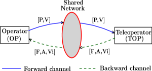
Figure 1: Schematic of a point-to-point telehaptic communication framework. Notations: [P, V] - [position, velocity], [F, A, Vi] - [force, audio, video].

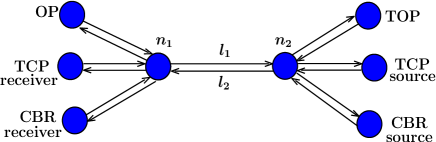
Figure 2: Single bottleneck network topology showing the telehaptic and cross-traffic sources and receivers. $l_{1}$ and $l_{2}$ - bottleneck links on forward and backward channels; $n_{1}$ and $n_{2}$ - intermediate nodes.

We now describe the framework of a typical point-to-point telehaptic communication system on a shared network, shown in Figure 2. The human operator (OP) controls the remote robotic manipulator known as the teleoperator (TOP). The OP transmits the current position and velocity commands on the forward channel. The TOP follows the trajectory of the OP through execution of the received commands. The resulting force feedback is transmitted back to the OP along with the captured audio and video signals on the backward channel. Note that the telehaptic communication is inherently bidirectional and asymmetric in nature.

1.2 Organization of the Article

This article is organized as follows. In Section 2, we provide a brief overview of the working principle of TCP, and present our proposed mathematical model for characterizing the interplay between TCP and CBR flows. In Section 3, we specialize our model for characterizing the QoS parameters for CBR-based telehaptic protocols. We validate our claims through rigorous simulations and network experiments in Section 4. In Section 5, we present our results on the interplay between a telehaptic communication protocol employing the adaptive sampling scheme and network cross-traffic. We address audio and video delays for CBR-based telehaptic protocols in Section 6. Finally, we review the related literature on the interplay between TCP and CBR traffic in Section 7, and conclude in Section 8.

2 TCP-CBR Interplay

TCP forms the backbone of a wide range of internet applications that demand reliable data transfer, such as web browsing, email, file download, and even video streaming applications like YouTube and Netflix. Studies show that TCP traffic constitutes over 90% of all internet traffic [Ryu et al. (2003), Yao et al. (2002)]. TCP is a transport layer protocol that controls the rate at which the application injects traffic into the network based on the perceived network conditions. It achieves end-to-end reliability through retransmission of lost packets, which are detected using packet acknowledgments (ACKs) that are sent to the source by the receiver. In this section, we provide an analytical characterization of the delay and the jitter encountered by a CBR stream co-existing with a TCP stream on a single bottleneck link. This analysis, which generalizes the work of [Sun et al. (2004)] on queue dynamics of a single TCP flow, is of independent interest, shedding light on the interplay between TCP and CBR streams in a network. Further, our results can be applied to analyze the performance of CBR-based steaming media applications on shared networks. In Section 3, we apply these results to analyze QoS compliance of CBR-based telehaptic protocols that coexist with TCP cross-traffic on a shared network.

We begin by providing a brief overview of TCP NewReno [Floyd et al. (2004)], which is the most widely deployed variant of TCP on the internet.

2.1 TCP Background

A TCP source maintains a variable called congestion window (denoted by $W$) that defines the number of TCP packets that are outstanding, i.e., transmitted but not yet acknowledged. The congestion window $W$ controls the rate at which TCP traffic is injected into the network – a higher $W$ corresponds to a higher transmission rate, and vice-versa. The TCP source increments $W$ by 1 every round trip time (RTT). This phase is commonly referred to as congestion avoidance in the literature. Once a packet loss is detected, TCP infers that the network is overloaded and cuts its transmission rate aggressively. This phase is referred to as fast retransmit, fast recovery in the literature, wherein the TCP source retransmits the lost packet and awaits the corresponding ACK. Once this ACK is received, the TCP source re-enters the congestion avoidance phase with an initial congestion window that is half the window size at the time the loss was detected.

To provide a concrete visualization of the rate adaptation, consider the single bottleneck network topology shown in Figure 2 with a single TCP source (we ignore telehaptic and CBR cross-traffic for now). Let $\mu$ denote the capacity (in kbps) of the bottleneck link $l_{2}$, and $B$ denote the queue size (in bytes) at the ingress of the bottleneck link ($n_{2}$). Let $\tau$ (in ms) denote the one-way propagation delay of the TCP flow. The reference [Sun et al. (2004)] demonstrates that in such a setting, the congestion window $W$ and the queue occupancy $Q$ on the bottleneck link exhibit a cyclic (periodic) variation, as shown in Figure 3a. The interval between $t_{1}$ and $t_{2}$ corresponds to the congestion avoidance phase. Note that $W$ is incremented in steps of 1, and the resulting increase in transmission rate causes the queue occupancy to increase. The duration between two consecutive updates in $W$ during the congestion avoidance is termed as a slot [Sun et al. (2004)]. Once a packet loss (due to queue overflow) is detected (at $t_{2}$), the source enters the fast retransmit, fast recovery phase. In this phase, corresponding to the interval between $t_{2}$ and $t_{3}$, the source retransmits the lost packet, and reduces its transmission rate aggressively causing the queue to drain quickly. Once the source receives the ACK corresponding to the retransmitted packet (at $t_{3}$), it re-enters the congestion avoidance phase, and the cycle repeats.

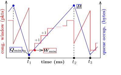
(a)

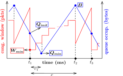
(b)

Figure 3: Evolution of TCP congestion window and bottleneck queue occupancy for (a) single TCP flow (b) heterogeneous flows involving single TCP flow and at least one CBR flow.

During the congestion avoidance phase, note that when an ACK arrives after the start of a slot the source transmits a packet to compensate for the packet that has left the network. On the other hand, at the start of a slot (when the congestion window is increased by 1) the source transmits two packets back-to-back. While the first one is the compensating packet, the second one adds an extra packet into the network for satisfying the updated $W$ value. We term this additional packet as the probing packet, since this packet probes the network for extra bandwidth. In other words, the source transmits a probing packet at the start of each slot. It is worth noting that the length of a slot is simply the RTT encountered by the corresponding probing packet.

Let $W_{min}$ and $Q_{min}$ denote the minimum value of $W$ and $Q$ in one cycle, respectively. The reference [Sun et al. (2004)] provides an analytical characterization of $W_{min}$ and $Q_{min}.$ Specifically, it is proved that if $B>2\mu\tau,$

$$Q_{min}=\frac{B-2\mu\tau}{2},\qquad W_{min}=\frac{B+2\mu\tau}{2S_{tcp}},$$

where $S_{tcp}$ is the size of a TCP packet.

In the following, we generalize the analysis in [Sun et al. (2004)] to include a CBR flow co-existing with the TCP flow on the bottleneck link. This non-trivial generalization leads to a characterization of (i) the maximum and minimum end-to-end CBR delay, (ii) the maximum CBR jitter. This characterization will be useful in our subsequent analysis of the interplay between heterogeneous cross-traffic and telehaptic stream.

2.2 TCP-CBR Interplay

For our analysis, we consider the same network setting as above, except that there are now two traffic flows on the network, a TCP flow and a CBR flow. Let $R$ denote the data rate of the CBR flow. For simplicity, we assume that the reverse channel (i.e., link $l_{1}$) is uncongested.

Assumptions: For the ease of our analysis, we follow [Sun et al. (2004)] and make the below assumptions.

1. The TCP source has an infinite backlog of data.

2. The access links to $l_{1}$ and $l_{2}$ have very high bandwidth and negligible propagation delays. In effect, the traffic sources (respectively, receivers) directly feed into (respectively, read from) $n_{2}$ (respectively, $n_{1}$).

3. The queue size at the ingress of the bottleneck link ($n_{2}$) is greater than the bandwidth-delay product of the TCP flow i.e., $B>2\mu\tau$. This condition guarantees that the queue never empties, and hence the bottleneck link is never underutilized [Villamizar and Song (1994)].

4. In every cycle, the TCP stream loses exactly one packet due to queue overflow at $n_{2}$.

2.2.1   Characterization of Queue Occupancy

Similar to the case of a single TCP flow in [Sun et al. (2004)]), it can be shown that in steady state $W$ and $Q$ vary periodically in time; see Figure 3b. However, the presence of the CBR traffic changes the nature of the queue occupancy evolution relative to the congestion window evolution. Note that during the congestion avoidance phase (the interval between $t_{1}$ and $t_{2}$), the queue occupancy initially decreases over $c_{1}$ slots, and then increases until an overflow occurs. Let $c$ denote the total number of slots in the congestion avoidance phase of each cycle.

Let $Q_{init}$ denote the queue occupancy at the start of the congestion avoidance phase. Let $i$ be the slot index, and $Q(i)$ denote the value of $Q$ at the start of $i$^th slot. Therefore, we can write $Q(1)=Q_{init}$. For brevity, we only present the key results of our analysis in this section. Interested readers can refer to Appendix 9.1 for a detailed description. From our analysis, we obtain closed form expressions for $W_{min},Q_{init}$, and $c$ as given by Equations (1), (2), and (3), respectively.

$$W_{min}=\frac{(B+2\mu\tau)(1-\alpha)}{2S_{tcp}},$$ (1)

$$Q_{init}=\frac{(B+2\mu\tau)(1+\alpha)}{2}-2\mu\tau,$$ (2)

$$c=\frac{(B+2\mu\tau)(1-\alpha)}{2S_{tcp}}+1,$$ (3)

where $\alpha:=\frac{R}{\mu}$. Additionally, the analysis also yields Equations (4) and (5) with unknowns $Q_{min}$ and $c_{1}$.

$$Q_{min}+\Big{[}\frac{(B+2\mu\tau)(1-\alpha)}{2S_{tcp}}-c_{1}+1\Big{]}\Big{[}\frac{S_{tcp}}{1-\alpha}\Big{]}=B$$ (4)

$$Q_{min}=\Big{[}\frac{(B+2\mu\tau)(1+\alpha)}{2}-2\mu\tau\Big{]}\alpha^{c_{1}}+\Big{[}\frac{(B-2\mu\tau)(1-\alpha^{c_{1}})}{2}\Big{]}+S_{tcp}\sum_{j=0}^{c_{1}-2}(c_{1}-1-j)\alpha^{j}$$ (5)

As can be noticed, $Q_{min}$ and $c_{1}$ do not admit a closed form characterization. However, they are easily amenable to numerical computation as follows. The evolution of the queue occupancy across slots during the congestion avoidance phase is given by:

$$\begin{split}Q(i)=\Big{[}\frac{(B+2\mu\tau)(1+\alpha)}{2}-2\mu\tau\Big{]}\alpha^{i-1}+\Big{[}\frac{(B-2\mu\tau)(1-\alpha^{i-1})}{2}\Big{]}+S_{tcp}\sum_{j=0}^{i-3}(i-2-j)\alpha^{j},\\ \forall i\in[1,c].\end{split}$$ (6)

Note that (5) is a special case of (6) setting $i=c_{1}+1$ (which corresponds to the queue occupancy after $c_{1}$ slots). Since $Q(\cdot)$ is unimodal over a cycle, $Q_{min}$ can be computed numerically by minimizing $Q(i)$ over $i\in[1,c].$ Therefore, we have

$$Q_{min}=\min_{i\in[1,c]}Q(i),\quad c_{1}=\operatorname*{arg\,min}_{i\in[1,c]}Q(i)-1.$$ (7)

As described previously, TCP rate adaptation is based on queue overflows which occur when the queue occupancy reaches the maximum permissible value $B$. This implies that the maximum queue occupancy $Q_{max}=B$. Therefore, we can write $Q(i)\in[Q_{min},Q_{max}]$.

To summarize, the above analysis characterizes the minimum and the maximum queue occupancy at the ingress of the bottleneck link in terms of network parameters ($\mu,\tau,B$) and the CBR source parameter $R$.

2.2.2   Characterization of CBR Delay

Based on the above results, we now move to the characterization of the end-to-end delay experienced by the CBR flow. The delay experienced by the CBR packets is composed of propagation delay and queueing delay. The latter is in turn proportional to the queue occupancy encountered by the CBR packet upon arrival into the queue at the bottleneck link. Thus, the minimum and the maximum end-to-end delay seen by CBR packets, denoted $d_{min}$ and $d_{max},$ respectively, are given by

$$d_{min} =\tau+\frac{Q_{min}}{\mu},$$ (8)

$$d_{max} =\tau+\frac{B}{\mu}.$$ (9)

To summarize, the CBR delays vary cyclically (in synchronization with the queue occupancy) over the range [$d_{min},d_{max}$]. We apply this delay characterization to determine the telehaptic delays (Section 3.1), and subsequently to derive sufficiency conditions for QoS compliance of telehaptic flows (Sections 4 and 5).

2.2.3   Characterization of CBR Jitter

We now move to characterizing the jitter experienced by the CBR flow in presence of TCP cross-traffic. Jitter refers to the variation in the inter-packet delay. Formally, we define the CBR jitter as

$$\delta_{cbr}=\Delta D_{j},$$

where $\Delta D_{i}$ refers to the difference between the end-to-end delays experienced by $j$^th and $(j-1)$^th CBR packets [Knoche and De Meer (1997)]. Therefore, the maximum CBR jitter is given as

$$\delta_{cbr(max)}=\max_{j}\Delta D_{j}.$$

Note that our definition of maximum jitter captures the largest positive difference between the end-to-end delays experienced by successive CBR packets. Indeed, for streaming applications, it is these positive delay differences that are troublesome; a negative delay difference only means that a sample arrived earlier than its nominal rendering time.

Since the only variable component of the end-to-end delay is the queueing delay, it follows that

$$\delta_{cbr(max)}=\max_{j}\frac{1}{\mu}\Delta Q_{j},$$

where $\Delta Q_{j}$ denotes the difference between the queue occupancy seen by $j$^th and $(j-1)$^th CBR packets. This results in the following characterization of the CBR jitter.

$$\delta_{cbr(max)}=\frac{1}{\mu}\left[m_{tcp}S_{tcp}+(R-\mu)T_{cbr}\right].$$ (10)

Here, $T_{cbr}$ refers to the interval between the transmission of successive CBR packets, and $m_{tcp}$ denotes the maximum number of packets transmitted by the TCP source in an interval of length $T_{cbr}$. Thus, all that remains is to characterize $m_{tcp}.$

At this stage, it is appropriate to describe the cumulative acknowledgement principle of TCP NewReno, as this governs the TCP parameter $m_{tcp}$. According to this principle, the TCP receiver transmits an ACK every $n$^th packet, where $n\geq 1$, thereby cumulatively acknowledging the reception of $n$ successive packets. Note that the description of the working of TCP in Section 2.1 corresponds to $n=1$. In general, a TCP source transmits a burst of $n$ packets when a (cumulative) ACK that acknowledges only compensating packets is received (this burst consists of $n$ compensating packets), and transmits a burst of $n+1$ packets when a (cumulative) ACK that acknowledges a probing packet is received (this burst consists of $n$ compensating packets and a probing packet). Note that packets transmitted in the same burst are not necessarily acknowledged simultaneously. Specifically, if there are $m<n$ unacknowledged packets at the receiver when a burst of $n$ packets arrives, then the receiver cumulatively acknowledges the older $m$ packets and the earliest $n-m$ packets in the current burst. The remaining $m$ packets of the current burst are cumulatively acknowledged when the next burst arrives.

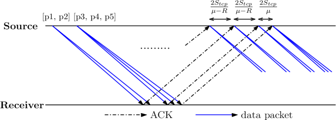
Figure 4: Demonstration of the working of cumulative ACK mechanism of TCP with $n=$ 2, along with the specification of inter-ACK gap. The packets are numbered sequentially in the order of their transmission, and the packets belonging to the same burst are grouped together using square brackets.

Since the source transmissions are triggered by ACK receptions, $m_{tcp}$ depends on the maximum number of ACKs that can be received by the source in an interval of length $T_{cbr}.$ Nominally, as we show in Figure 4 with $n=$ 2 (explained in detail in Appendix 9.2), the interval between successive ACK receptions at the source equals $\frac{nS_{tcp}}{\mu-R}$, if the ACKs acknowledge only the probing packets. However, at a slot boundary, the two ACKs are received with a (smaller) time gap of $\frac{nS_{tcp}}{\mu}$ due to the following: Suppose that there are $n-1$ unacknowledged packets at the receiver when the burst of $n+1$ packets containing a probe packet is received. In this case, the burst would trigger two ACKs from the receiver, one to acknowledge the $n-1$ older packets and the first packet of the current burst, and another to acknowledge the remaining $n$ packets of the current burst. It is important to note the following.

• The two ACKs would be received $nS_{tcp}/\mu$ time units apart, since this is the time required for $n$ back-to-back packet receptions at the receiver.

• The first ACK would trigger a transmission of $n-$packet burst from the source, while the second (which acknowledges a probing packet) would trigger a transmission of $(n+1)-$packet burst.

Thus, $m_{tcp}$ is given by

$$m_{tcp}=n+1+n\Bigg{(}1+\left\lfloor\frac{T_{cbr}-\frac{nS_{tcp}}{\mu}}{\frac{nS_{tcp}}{\mu-R}}\right\rfloor\Bigg{)}I_{\big{(}T_{cbr}>\frac{nS_{tcp}}{\mu}\big{)}},$$ (11)

where $I_{z}=$ 1 if $z=$ 1, and 0 otherwise. Here, the term $n+1$ is due to the packets in the $(n+1)-$packet burst. The term inside the parenthesis represents the maximum number of $n-$packet bursts that can be transmitted in the interval of length $T_{cbr}$ in addition to the $(n+1)-$packet burst. In other words, it is the maximum number of $n-$packet bursts transmitted in an interval of length $T_{cbr}-\frac{nS_{tcp}}{\mu}$.

From Equations (10) and (11), the maximum jitter experienced by the CBR stream is given as

$$\delta_{cbr(max)}=\frac{S_{tcp}}{\mu}\Bigg{[}n+1+n\Bigg{(}1+\left\lfloor\frac{T_{cbr}-\frac{nS_{tcp}}{\mu}}{\frac{nS_{tcp}}{\mu-R}}\right\rfloor\Bigg{)}I_{\big{(}T_{cbr}>\frac{nS_{tcp}}{\mu}\big{)}}\Bigg{]}+\frac{RT_{cbr}}{\mu}-T_{cbr}.$$ (12)

The above characterization allows us to express the maximum jitter of CBR stream in terms of a set of source parameters ($n,S_{tcp},T_{cbr},R$) and a network parameter $\mu$. Interestingly, $\delta_{cbr(max)}$ has no dependence on other network parameters like $B$ and $\tau,$ both of which influence the delay profile significantly. Therefore, we conclude that unlike CBR delay, maximum CBR jitter is primarily source-driven.

3 CBR-based Telehaptic Protocols: QoS Characterization

In this section, we apply the analytical characterization of TCP-CBR interplay in Section 2 to analyse the QoS experienced by CBR-based telehaptic flows in the presence of heterogeneous cross-traffic. For concreteness in exposition, we assume that the (CBR based) telehaptic flow encounters one TCP and one CBR cross-traffic flow over the bottleneck link in the network topology shown in Figure 2. Let $R_{h}$ and $R_{cross}$ denote the rates of the telehaptic stream and the CBR cross-traffic stream, respectively. Note that the aggregate rate of CBR cross-traffic as seen by the TCP source (using the notation of Section 2) equals $R=R_{h}+R_{cross}.$ Finally, let the inter-packet gap of telehaptic stream be denoted by $T_{h}$, and the packet size of CBR cross-traffic be denoted by $S_{cross}$.

3.1 Characterization of Haptic Delay

The maximum and the minimum delay experienced by telehaptic packets follow directly from the analysis in Section 2. Indeed, the characterization of the minimum queue occupancy $Q_{min}$ on the bottleneck link depends on the aggregate rate $R$ of the CBR cross-traffic seen by the TCP source (and not on the composition of the CBR cross traffic). Thus, Equations (8) and (9) also determine the minimum and the maximum delays encountered by the telehaptic packets, respectively. In other words, haptic delays vary cyclically in the range $[d_{min},d_{max}]$. We validate these bounds through simulations and real network experiments in Sections 4.1.1 and 4.2.1, respectively.

3.2 Characterization of Haptic Jitter

Next, we turn to the characterization of the maximum jitter experienced by the telehaptic packets. It is important to note that in practice, negative haptic jitter (caused by decreasing haptic delays) are canceled using a jitter buffer at the receiver. The jitter buffer delays the play-out of the received samples such that the rendering jitter is minimized. Therefore, in this paper, we focus only on positive haptic jitter, (as discussed in Section 2.2.3), which has the potential to impair human perception during a telehaptic activity.

Unlike delay, the jitter experienced by the two CBR streams (the telehaptic stream and the cross-traffic stream with rate $R_{cross)}$) will in general be different. This is because the jitter of each stream is determined by the maximum cross-traffic injected into the queue between successive packets of that stream. Accordingly, in the following, we adapt the jitter characterization in Section 2.2.3 to obtain an expression for the maximum haptic jitter.

Analogous to Equation (10), the maximum haptic jitter can be expressed as

$$\delta_{h(max)}=\frac{1}{\mu}[m_{tcp}S_{tcp}+m_{cross}S_{cross}+(R_{h}-\mu)T_{h}],$$

where $m_{cross}$ denotes the maximum number of CBR cross-traffic packets transmitted within an interval of length $T_{h}$. The numerator in the above expression indicates the maximum increase in the queue occupancy between the arrival of two successive telehaptic packets. Analogous to Equation (11), we can write the maximum number of TCP packets that can be transmitted in the interval $T_{h}$ as

$$m_{tcp}=n+1+n\Bigg{(}1+\left\lfloor\frac{T_{h}-\frac{nS_{tcp}}{\mu}}{\frac{nS_{tcp}}{\mu-R}}\right\rfloor\Bigg{)}I_{\big{(}T_{h}>\frac{nS_{tcp}}{\mu}\big{)}}.$$

Moreover, it is easy to see that

$$m_{cross}=\left\lceil\frac{R_{cross}T_{h}}{S_{cross}}\right\rceil.$$

Combining the above equations, the maximum haptic jitter is given by

$$\delta_{h(max)}=\frac{\Bigg{[}n+1+n\Bigg{(}1+\left\lfloor\frac{T_{h}-\frac{nS_{tcp}}{\mu}}{\frac{nS_{tcp}}{\mu-R}}\right\rfloor\Bigg{)}I_{\big{(}T_{h}>\frac{nS_{tcp}}{\mu}\big{)}}\Bigg{]}S_{tcp}+\left\lceil R_{cross}T_{h}\right\rceil+R_{h}T_{h}}{\mu}-T_{h}$$ (13)

We validate Equation (13) experimentally in Sections 4.1.2 and 4.2.2.

4 CBR-based Telehaptic Protocols: Experimental Results

The goal of this section is to validate our analysis presented in Section 3, and to subsequently develop an understanding of the conditions required for QoS-compliant telehaptic communication on a shared network for CBR based telehaptic protocols.

In the first part of this section, we use NS3 – a discrete event network simulator for validating our analytical model. We find that our delay and jitter bounds are fairly accurate over a wide range of network settings. We also make the empirical observation that telehaptic packet losses are rare so long as the packet sizes are small relative to TCP packets. The above observations lead us to formulate a comprehensive set of conditions for QoS-compliant telehaptic communication on shared networks.

To further test the validity of our conclusions under real network conditions, we also conducted rigorous experiments on a real network. The results of these experiments are presented in the second part of this section. The delay and packet loss observations match with those in the simulations. Interestingly, we find a mismatch between the the measured jitter in these experiments and our analytical jitter bound. We are able to trace these errors to differences between the implementation of TCP NewReno in the employed operating system and the RFC specification. We conclude that telehaptic jitter is highly sensitive to variations in the implementation of TCP in the operating systems of the sender/receiver.

The experimental settings that follow apply to both simulations as well as network experiments. We employ the single bottleneck network topology shown in Figure 2. Unless otherwise specified, we use the following network settings throughout this section. We set $\mu=$ 6 Mbps, $\tau=$ 8 ms and $B=$ 14 kB. We work with real haptic traces generated by the Phantom Omni device [Sensable (2012)] which offers a single point of interaction between the human user and the haptic environment. Considering the standard haptic sampling rate of 1 kHz, and accounting for the overhead due to packet headers, we get a forward channel data rate $R_{f}=$ 688 kbps, with packets of size 86 bytes transmitted every millisecond [Gokhale et al. (2015)]. On the backward channel, we simulate audio and video payload at the rate of 64 kbps and 400 kbps, respectively. We consider the media multiplexing mechanism proposed in [Gokhale et al. (2015)], where each packet contains a single haptic sample and an audio/video fragment of a fixed size. Accounting for the the packet header overhead leads to a backward channel data rate $R_{b}=$ 1.096 Mbps, with packets of size 137 bytes transmitted every millisecond.

For brevity, we report the results for the case in which cross-traffic sources are added to the backward channel only. We introduce a TCP NewReno source with the standard packet size $S_{tcp}=$ 578 bytes. We also add a CBR cross-traffic source with packet size $S_{cross}=$ 150 bytes. In the notation of Section 2.2, note that the aggregate CBR rate on the backward channel $R=R_{b}+R_{cross}.$ For sustaining the TCP flow throughout the duration of the experiment, we need to ensure that $R<\mu$ so that the TCP flow has sufficient network bandwidth to perform rate adaptation. Our simulations and network experiments are performed for a duration of 500 seconds. Due to the fact that QoS requirements of delay and jitter for haptic samples are stricter than those for audio/video, we only report haptic delay and jitter measurements in this section. We discuss audio/video QoS compliance in Section 6. However, we report the packet loss measurements for all three media types.

4.1 Simulations

In this section, we present the validation results of our analysis through simulations.

4.1.1   Haptic Delay

In our simulations, we observe that the TCP congestion window exhibits steady behavior only if $R<$ 5.5  Mbps. Hence, we restrict our measurements to a maximum CBR rate of $R=$ 5.5 Mbps, since our analysis applies only to steady state TCP dynamics. In Table 2, we report the minimum and the maximum haptic delays as measured in the simulations and the corresponding analytical bounds (stated in Section 3.1) by varying $R_{cross}$ to get $R$ in the range [$R_{b}$, 5.5 Mbps]. Throughout this range, we see that while the analytical lower bound $d_{min}$ has a modest accuracy, the upper bound $d_{max}$ is highly accurate.

$R$ (Mbps)	$d_{min}$ (ms)		$d_{max}$ (ms)
	A	S	A	S
1.096	9.91	8.89	26.66	26.47
2	10.74	9.21	26.66	26.40
3	12.27	11.71	26.66	26.62
4	14.81	12.95	26.66	26.45
5	19.87	16.95	26.66	26.55
5.5	22.68	19.77	26.66	26.43

Table 2: Comparison of $d_{min}$ and $d_{max}$ by analysis (A) and simulation (S) for a wide range of $R$.

$\mu$ (Mbps)	$\delta_{h(max)}$ (ms)
	A	S
9	1.46	1.46
12	1.62	1.61
15	1.09	1.09
18	0.84	0.85
21	0.49	0.49
25	0.63	0.62

Table 3: Comparison of $\delta_{h(max)}$ by analysis (A) and simulation (S) for a wide range of $\mu$.

In Figure 6, we plot the temporal variation of the haptic delay for $R=$ 3 Mbps (i.e., $R_{cross}=$ 1.904 Mbps), along with the analytical bounds. Note that the haptic delay evolves periodically over time, matching our analytical upper and lower bounds.

We make the following remarks.

• The upper bound $d_{max},$ which is insensitive to $R,$ is highly accurate. However, the lower bound $d_{min}$ becomes inaccurate as $R$ approaches $\mu$. This is because our characterization of $d_{min}$ assumes a single TCP packet loss in each cycle; see Assumption (4) in Section 2.2. However, we observe in our traces that as $R$ approaches $\mu$, TCP starts to lose multiple packets per cycle, leading to a very different congestion window evolution from the one analyzed. Simulating a wide range of network settings, we observe that a sufficient condition for a single TCP packet loss per cycle (and consequently for the accuracy of $d_{min}$) is $R\leq 0.65\mu.$

• Since the analytical upper bound $d_{max}$ is highly accurate, it can be used to check for QoS-compliance of the haptic delay for a given network setting, i.e. $d_{max}<$ 30 ms. In the network setting under consideration, $d_{max}=$ 26.66 ms which is less than the QoS limit of 30 ms. Indeed, our measurements confirm that the haptic delay constraint is satisfied in this case.

To see another example, consider the following setting: $\mu=$ 6 Mbps, $\tau=$ 15 ms, and $B=$ 45 kB. In this case, using (9), we obtain $d_{max}=$ 75 ms, which suggests that the haptic delay constraint cannot be met. Indeed, simulations show that this is the case; see Figure 6. Thus, the expression for $d_{max}$ can be used to identify the class of network settings where the QoS-compliance of the haptic delay is feasible.

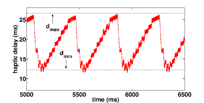
Figure 5: Plot of haptic delay showing the corroboration between analytical estimate and simulation measurement.

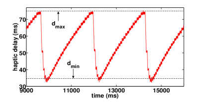
Figure 6: Plot of haptic delay demonstrating the severe QoS violation for a particular network setting.

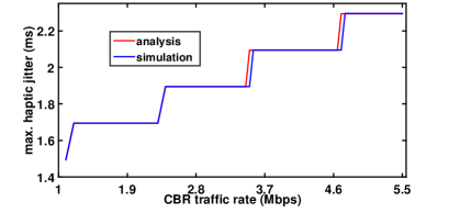
Figure 7: Plot demonstrating the corroboration between theoretical estimates and simulation measurements of maximum haptic jitter.

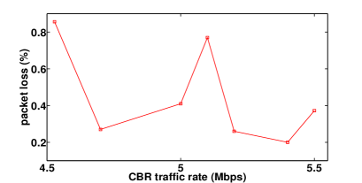
Figure 8: Packet losses recorded on the backward channel for a case where the telehaptic packet sizes are comparable to the TCP packet sizes.

4.1.2   Haptic Jitter

We now turn to measurements of the maximum haptic jitter. Figure 8 shows the maximum haptic jitter curves, both by analysis and simulation, for $R\in[R_{b},5.5$ Mbps$]$. It can be seen that the analytical estimates corroborate well with the simulation measurements, thereby validating our characterization. It is to be noted that the indicator variable $I_{(T_{h}>\frac{nS_{tcp}}{\mu})}$ in Equation (13) takes the value 0 for the chosen setting, i.e., $T_{h}<nS_{tcp}/\mu$. In order to test the robustness of our model to the network parameters, we choose another setting that results in $I_{(T_{h}>\frac{nS_{tcp}}{\mu})}=$ 1. Specifically, we use $\mu$ as the control parameter and vary it in the range [9, 25] Mbps. Also, we set $R_{cross}=$ 6.9 Mbps, so that $R=$ 8Mbps. In Table 3, we report the maximum haptic jitter by analysis (A) and simulation (S). Throughout the considered range of $\mu$, it can be seen that our analysis accurately estimates the maximum haptic jitter.

4.1.3   Packet Loss

We now report the the packet loss suffered by the telehaptic stream. Interestingly, for all our simulations reported so far, we notice that telehaptic packet losses are zero in spite of the regular queue overflows induced by TCP. The rationale behind this interesting behavior is that the telehaptic source generates smaller packets compared to the TCP packets (137 bytes per packet on the backward channel for the telehaptic stream, versus 578 bytes per packet for the TCP stream). As a result, even when the queue drops a TCP packet, the adjacent telehaptic packets can still (potentially) be accommodated in the queue. This observation is in line with the results in [Sawashima et al. (1997)], which also investigates CBR loss in the presence of TCP cross-traffic.

To confirm our conjecture that smaller telehaptic packet sizes are responsible for the absence of telehaptic packet losses, we simulate a scenario with higher resolution haptic, audio, and video devices, so that the telehaptic packet size becomes comparable to the TCP packet size. Specifically, consider a haptic device like Cybergrasp [Immersion (2003)] or Festo’s exohand [Festo (2013)]. Assuming two interaction points for each of the ten fingers of the hands results in a twenty-fold increase in the haptic payload rate. Additionally, we simulate high-definition audio and video payload with rates of 128 kbps and 2 Mbps, respectively. This results in $R_{b}=$ 4.528 Mbps, and a packet size of 566 bytes on the backward channel for every millisecond. Note that the telehaptic packets are now comparable in size to the TCP packets. Figure 8 presents the packet loss (in %) encountered by this telehaptic stream, where we vary $R_{cross}$ to get $R$ in the range $[R_{b},$ 5.5 Mbps]. Note that with the larger telehaptic packets, losses do occur. While the measured telehaptic losses pose no threat to haptic media (with a QoS limit of 10%), audio and video (which have a more stringent limit of 1%) are more susceptible to QoS violations.

To summarize, if telehaptic packets are small relative to TCP packets, the telehaptic stream sees little or no packet loss. However, if the telehaptic packets become comparable in size to TCP packets (due to higher fidelity media devices), packet losses become noticeable.

In conclusion, we see that for QoS-compliant communication under CBR-based telehaptic protocols, the following conditions need to be satisfied.

• For buffer stability, we naturally require that the aggregate CBR data rate is less than the link capacity, i.e., $R<\mu.$

• In order to satisfy the haptic delay constraint, we need $d_{max}<30$ ms, i.e.,

  $$\tau+\frac{B}{\mu}<30.$$ (14)

• In order to satisfy the haptic jitter constraint, we need to configure the source and the network parameters such that $\delta_{h(max)}<$ 10 ms, where $\delta_{h(max)}$ is given by Equation (13).

• To avoid loss in the presence of concurrent TCP traffic, the packet sizes used by the telehaptic protocol should be small relative to the TCP packet sizes.

4.2 Network Experiments

In order to validate our model under real network conditions and with real implementations of TCP NewReno in Debian operating system (kernel version 4.14), we perform experiments on a real network setup using the single bottleneck network topology that we used earlier (shown in Figure 2). Each node in the topology is run on a virtual machine created using the VMware virtualization infrastructure. We install the virtualization software on two workstations, each of which hosts multiple virtual machines. The virtual machines corresponding to the traffic sources and the adjoining intermediate node ($n_{2}$) are installed on the same workstation, and the remaining nodes are installed on another workstation. The two workstations are distantly located from each others, and are connected via a physical network.

The network parameters are configured as per our simulation settings ($\mu=$ 6 Mbps, $\tau=$ 8 ms, and $B=$ 14 kB) using the NetEm tool which is a standard built-in Linux kernel feature for network emulation. The CBR traffic (telehaptic and cross-traffic) is generated using socket programs running on the corresponding sources, whereas the TCP NewReno traffic is generated using the Iperf tool [Tirumala (1999)]. We note that the TCP NewReno implementation uses minimum packet size of 1512 bytes (further details explained in Section 4.2.2), and $n=$ 2.

4.2.1   Haptic Delay

We begin by presenting the minimum and the maximum haptic delay measurements in our network experiments. As in the measurements corresponding to Table 2, we vary $R_{cross}$ to get $R$ in the range [$R_{b},5.5$ Mbps]. In Table 4, we report $d_{min}$ and $d_{max}$ measured in our network experiments (E). For ease of comparison, we also present the delays corresponding to analysis (A) and simulations (S) that we reported earlier in Table 2. It can be seen that the delay measurements corroborate well with the analytical estimates, thereby validating the accuracy of our delay analysis model under real network conditions as well. Note that the Linux implementation of TCP NewReno uses larger packet sizes, and hence the queue starts to drop packets at a lower queue occupancy than in simulations. This results in a lower $d_{max}$ in network experiments.

$R$ (Mbps)	$d_{min}$ (ms)			$d_{max}$ (ms)
	A	S	E	A	S	E
1.096	9.91	8.89	8.34	26.66	26.47	22.17
2	10.74	9.21	8.79	26.66	26.40	22.58
3	12.27	11.71	11.46	26.66	26.62	23.29
4	14.81	12.95	12.42	26.66	26.45	23.09
5	19.87	16.95	17.13	26.66	26.55	24.58
5.5	22.68	19.77	20.06	26.66	26.43	24.69

Table 4: Comparison of $d_{min}$ and $d_{max}$ by analysis (A), simulation (S), and real network experiments (E) for a wide range of $R$.

$R$ (Mbps)	$\delta_{h(max)}$ (ms)
	A	E
1.096	5.43	10.62
2	5.63	10.94
3	5.83	11.27
4	6.03	11.44
5	6.23	7.87
5.5	6.23	6.03

Table 5: Analytical (A) and experimental (E) measurements for $\delta_{h(max)}$ over a wide range of $R$.

4.2.2   Haptic Jitter

We now move to maximum haptic jitter measurements. As shown in Equation (13), $\delta_{h(max)}$ has a direct dependence on $S_{tcp}$. We compute the $\delta_{h(max)}$ with $S_{tcp}=$ 1512 B for different values of $R_{cross}$ using Equation (13). In Table 5, we present the analytical estimates (A) and their corresponding experimental measurements (E) of $\delta_{h(max)}$. As can be seen, there exists considerable error between the two quantities.

We now explain the rationale behind this error. From our traces, we notice that the TCP NewReno implementation in Debian operating system deviates from the definition in the RFC [Floyd et al. (2004)] as follows:
$S_{tcp}$ is implemented as a dynamic parameter that depends on the value of $W_{min}$. When $W_{min}$ is low, which corresponds to low bandwidth availability in the network, the source transmits packets of (smaller) size $S_{tcp}=$ 1512 B. On the other hand, when $W_{min}$ is high, which corresponds to high bandwidth availability, the source increases the packet size to $S_{tcp}=$ 2960 B. For intermediate values of $W_{min},$ the source transmits a mix of small and large packets.

As a consequence, the amount of traffic (in bytes) injected by the TCP source into the network at a slot boundary, which as we have seen determines $\delta_{h(max)}$, depends on $W_{min}$. We can now explain the deviation of $\delta_{h}(E)$ from $\delta_{h}(A)$ as follows. When $R$ is small, we expect $W_{min}$ to be high (as per Equation (1)). Therefore, at the slot boundaries the source transmits three larger packets resulting in higher $\delta_{h(max)}$. It is worth noting that for $R\in$ [1.096, 4] Mbps, simply by assigning $S_{tcp}=$ 2960 B, $\delta_{h(max)}(A)$ precisely matches $\delta_{h(max)}(E)$. As $R$ is increased further, the source gradually starts to transmit smaller packets. For example, when $R=$ 5 Mbps, we observe that one larger and two smaller packets are transmitted at the slot boundaries. This results in diminishing error between $\delta_{h(max)}(E)\text{ and }\delta_{h(max)}(A)$. When $R=$ 5.5 Mbps, three smaller packets are transmitted, resulting in a negligible error between the two.

We conclude that the maximum haptic jitter is highly sensitive to the implementation aspects of TCP NewReno. While our analysis assumes the dynamics specified in the RFC [Floyd et al. (2004)], the actual implementation in the Debian operating system deviates from the RFC, resulting in a mismatch between the analytical and the experimental jitter. Coming up with an analytical bound for the haptic jitter that is robust to the specifics of common TCP implementations is an interesting avenue for future work.

4.2.3   Packet Loss

The telehaptic packet losses in all of our network experiments are zero. Note that this is because the bottleneck queue can still admit smaller sized telehaptic packets while it drops the larger sized TCP packets. Note that the TCP packets here are larger compared to those in simulations.

5 Adaptive Sampling based Telehaptic Protocols

In this section, we study the interplay between adaptive sampling based telehaptic protocols and heterogeneous cross-traffic involving TCP and CBR flows. An adaptive sampling scheme based protocol transmits only perceptually significant haptic samples on the forward and/or backward channels. As before, the goal of this section is to evaluate the impact of network cross-traffic on telehaptic traffic generated by the adaptive sampling based telehaptic protocols. This also leads to formulating the conditions for QoS-compliant telehaptic communication.

If the protocol employs Weber sampler [Hinterseer et al. (2008)], a specific type of adaptive sampling strategy, on the backward channel, it must also specify how the irregularly spaced, perceptually significant haptic samples are multiplexed with audio/video data. For a working example, we consider the visual-haptic multiplexing protocol [Cizmeci et al. (2014)], which multiplexes haptic and video streams on the backward channel as follows: The perceptually significant haptic samples are packetized with video data of worth 1 ms, so that the haptic samples suffer minimal packetization delay. On the other hand, when a series of haptic samples are perceptually insignificant, the protocol packs a large chunk of a video frame, not exceeding data of worth 15 ms, into a single packet for transmission.

In order to evaluate the protocol with realistic data, we record ten pilot signals collected from Phantom Omni device during a real telehaptic activity. For brevity, we report the results only for one of these traces, but we note that our findings remain consistent across traces. The video payload rate is set to 400 kbps, as before. We use the network settings described previously in Section 4.

In Figure 10, we plot the instantaneous telehaptic transmission rate on the backward channel due to visual-haptic multiplexing protocol. As can be seen from the figure, the instantaneous rate exhibits large fluctuations in the range [613, 1079] kbps, while the long term average rate of 712 kbps is substantially lower compared to the peak instantaneous rate (1079 kbps). We now move to our investigation of the interplay between this telehaptic flow and network cross-traffic. We begin by investigating the impact of CBR cross-traffic alone on the telehaptic traffic (Section 5.1), and then move to heterogeneous cross-traffic case (Section 5.2).

5.1 CBR Cross-Traffic

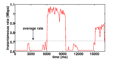
Figure 9: Instantaneous telehaptic data rate exhibiting rapid fluctuations under visual-haptic multiplexing.

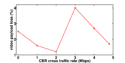
Figure 10: Video payload loss in presence of heterogeneous cross-traffic under visual-haptic multiplexing.

In this section, our goal is to demonstrate that from the standpoint of QoS compliance on a shared network, the statistical compression provided by adaptive sampling offers no meaningful economies in terms of network bandwidth requirement of the telehaptic application. In other words, the network has to be able to support the peak transmission rate of the telehaptic flow for QoS compliance.

To illustrate this, we consider an example where the network is provisioned for the long term average telehaptic rate. This means that the amount of network bandwidth available for the telehaptic stream at all times exceeds its average rate. To simulate this scenario, we set $R_{cross}=$ 5.28 Mbps so that the bandwidth available to the telehaptic stream is 720 kbps which is greater than the average rate of 712 kbps, as shown in Figure 10. We remove the TCP source for this experiment. In Figure 10, consider the interval between 6000 ms and 10000 ms, when the instantaneous rate exceeds the available bandwidth. In this interval, our simulation traces reveal a significant haptic and video payload losses of around 6.2%. Even though the haptic loss is below the QoS limits (10%), the video loss is alarmingly high, causing severe violations of the QoS requirement (1%). Additionally, we note that the haptic delay severely violates the Qos limit of 30 ms. As another example, setting $\mu=$ 3 Mbps and $R_{cross}=$ 2.28 Mbps results in larger haptic and video payload losses of around 9.6%.

This suggests that for Qos compliance, the network needs to be provisioned for the peak telehaptic rate rather than the long term average rate. Hence, the statistical (but network-unaware) compression achieved by adaptive sampling is not particularly effective from the standpoint of reducing the bandwidth requirement of the telehaptic application. This departure from the existing theories on adaptive sampling schemes, for example [Hinterseer et al. (2008), Clarke et al. (2006)], is another key contribution of this work, since the previous studies treat the long term average data rate as the primary parameter in the evaluation of quality of a telehaptic interaction.

5.2 Heterogeneous Cross-Traffic

For the case of heterogeneous cross-traffic, we reinstate the TCP source on the backward channel. Since $R_{b}\in$ [613, 1079] kbps, we vary $R_{cross}$ in the range [0, 4.4] Mbps so that $R\in$ [$R_{b}$, 5.5 Mbps]. Due to space limitations, we only state our main findings:

1. Equation (14) captures the peak delay seen by telehaptic packets accurately.

2. Figure 10 shows the video payload loss (in %) recorded for various values of $R_{cross}$. It can be seen that the video loss faces severe QoS violations throughout. This is because the visual-haptic multiplexing protocol transmits large packets with video payload in the absence of perceptually significant haptic samples. Recall, from our discussion in Section 4.1.3, that large packets are more likely to get dropped in the presence of TCP cross-traffic. Interestingly, haptic media suffers zero losses in this case. This is because the protocol transmits the perceptually significant samples in smaller packets of size 137 bytes. Once again, this illustrates that the packet sizing performed by a telehaptic protocol plays a crucial role in influencing the loss experienced in the presence of TCP cross-traffic.

Note that we do not discuss jitter in this section, since haptic jitter is harder to define under adaptive sampling, which only transmits perceptually significant samples that are irregularly placed in time.

To summarize, the conditions for QoS compliance for adaptive sampling based telehaptic protocols are:

• The network be provisioned for the peak telehaptic rate in order to alleviate the effects of the large fluctuations in the instantaneous telehaptic rate.

• To meet the haptic delay constraint, Equation (14) be satisfied.

• To avoid packet loss in presence of a TCP flow, large packet sizes be avoided.

6 Delay QoS Compliance for Audio-Video

While the previous sections have largely focused on haptic QoS compliance, we consider audio/video QoS compliance in this section. The goal of this section is to show that meeting the haptic delay requirement for CBR based telehaptic protocols typically guarantees that the (less stringent) delay requirements for audio and video are also satisfied under reasonable multiplexing schemes.

Since the relationship between haptic delay and audio-video delay depends strongly on the multiplexing framework being employed, we consider a specific example – the hierarchical multiplexing scheme developed in [Gokhale et al. (2017)]; an analogous analysis can also be performed for other multiplexing mechanisms. The multiplexing mechanism in [Gokhale et al. (2017)] is the following: An audio/video fragment of fixed size $s_{m}$ (in bytes) is transmitted along with each haptic sample, with audio payload having strict priority over video payload. With the assumption that the haptic delay deadline of 30 ms is met, we can derive the following expressions for the maximum delay experienced by the audio and the video frames.

$$d_{aud}=30+\frac{s_{a}}{s_{m}}T_{h},\qquad d_{vid}=30+\frac{1}{f_{v}},$$

where $s_{a}$ (in bytes) is the size of an audio frame, $f_{v}$ (in Hz) denotes the frame rate of the video signal, and $T_{h}$ is the inter-packet gap of telehaptic stream as before; see the reference [Gokhale et al. (2017)] for more details on this.

For the setting considered in Section 4, it can be shown that $s_{a}=$ 160 bytes, $s_{m}=$ 58 bytes, and $f_{v}=$ 25 Hz. Hence, $d_{aud}=$ 32.75 ms and $d_{vid}=$ 70 ms. We see that even the worst case audio and video delays are comfortably within their respective QoS limits. Thus, we conclude that compliance with the haptic delay constraint (which follows from Equation (14)) implies compliance with the delay constraints for audio and video media as well.

7 Related Work

In this section, we discuss the prior works relevant to this paper. Surprisingly, we note that there are no works that make a detailed examination of the interplay between telehaptic and TCP flows. A few works, however, have included TCP flows in their investigation, but the analyses themselves are rather trivial to draw any broad conclusions [Wirz et al. (2008), Gokhale et al. (2016)]. In the rest of this section, we present a brief review of the literature focused on the interplay between generic UDP (voice or video) and TCP flows.

7.0.1   Impact on TCP Flows:

A large volume of work is present in the literature in which the sole performance metric is TCP throughput. The work in [Doshi and Cao (2003)] provides an understanding of the network bandwidth sharing between multimedia streaming and TCP flows. In [Zahedi and Pahlavan (2000), Gupta et al. (2002), Aad et al. (2008), Bruno et al. (2008)], the authors discuss the impact of UDP flows on TCP throughput in wireless adhoc networks or LANs. The authors in [Gupta et al. (2004)] present a novel mechanism to enhance the TCP throughput in presence of concurrent UDP flows. The work in [Rohner et al. (2005)] demonstrates that the interaction of UDP and TCP on multihop wireless networks can result in significantly low throughput and unstable routes. The authors in [Suznjevic et al. (2014)] investigate the effect of UDP flows on the online gaming flows that are TCP-based, again with an emphasis on TCP throughput. The authors in [Beritelli et al. (2003), Bu et al. (2006)] investigate the impact of Voice over IP (VoIP) traffic on TCP traffic. A few works have proposed protocol designs for UDP-based traffic that yield to TCP flows in a fair manner; see, for example, [Rejaie et al. (1999), Rhee et al. (2000), Handley et al. (2002)]. It is important to remark that none of the prior works discussed so far focus on the impact of TCP traffic on the QoS experienced by the UDP flow.

7.0.2   Impact on UDP Flows:

As the multimedia streaming and tele-conferencing applications (both typically use UDP) gradually started gaining popularity, studies concerning the impact of TCP on UDP flows became the center of gravity for many research groups. The primary performance metrics of interest in these studies are the following: delay, jitter, and packet loss. In the rest of this section, we systematically discuss the prior works considering each of these metrics one-by-one.

Delay: The work in [Veres et al. (2001)] explores the possibility of providing differentiated services to voice, video, and data traffic with an objective of guaranteeing simultaneous delay QoS-compliance to media applications in a wireless network setting. A non-exhaustive list of works that carry out further investigations in this direction are [Arranz et al. (2001), Shetiya and Sharma (2005), Zhai et al. (2006), Papadimitriou and Tsaoussidis (2006), Boggia et al. (2007), Andreadis et al. (2008), Kim et al. (2009)]. In [Chen et al. (2006)], the authors employ a Markov chain model to estimate the average delay when UDP traffic shares the network resources with TCP streams on a wireless LAN. Recent investigations in this direction [De Cicco et al. (2011), Zhang et al. (2013)] employ the popular tele-conferencing tool Skype (which uses UDP) for studying its interplay with TCP traffic. These works report the long-term average RTT encountered by the Skype packets. Note that in each of the above studies, only the average delay is considered as the performance metric for real-time voice and/or video traffic. However, we remark that for ultra-sensitive telehaptic applications the instantaneous delay is a more meaningful evaluation metric than the time-average delay.

A few recent studies report the instantaneous delay of UDP packets under the influence of TCP flows. The authors in [Xu et al. (2012)] study voice and video delays with popular video telephony applications Google+, iChat, and Skype. Similar investigations have been carried out with a recently proposed protocol named Google Congestion Control (GCC) in [De Cicco et al. (2013), Carlucci et al. (2014)]. It is worth noting that all of the above works merely report the measured instantaneous UDP delays for the considered network settings.

To summarize, all of the above studies take into consideration only the experimental measurement of the UDP delays. It is imperative to point out that a theoretical characterization that provides a general model for the observed UDP delay profiles is lacking in the literature. Further, hitherto no work has considered investigating the conditions for meeting the delay deadline for haptic modality, which is more challenging compared to audio and video delay criteria.

Jitter: Several works like [Bonald et al. (2000), He and Chan (2003), Lin and Lai (2007)] have attempted to examine the time-average jitter suffered by a generic UDP streams due to coexisting TCP cross-traffic. Under similar settings, the authors in [Wong and Donaldson (2003)] have reported the average jitter encountered by voice and video streams. However, similar to delay, the more relevant parameter of interest is the instantaneous jitter which the above works do not explore. The reference [Cheng et al. (2008)] presents the instantaneous jitter faced by video streams in presence of TCP and other UDP streams. However, their investigation is based only on experimental observations; a mathematical model for characterization of the jitter is missing.

The authors in [Karam and Tobagi (2002)] experimentally investigate the impact of different packet scheduling schemes, like priority queueing and weighted round robin, on video jitter. In contrast, in this article, we consider droptail scheduling, which is a widespread form of packet scheduling in the internet. The work in [Daniel et al. (2003)] develops a statistical model for simulating jitter behavior in packet networks. However, both these works do not take the TCP rate dynamics into account.

Packet Loss: The first known effort in analyzing the UDP packet losses under the effect of TCP streams was carried out in [Sawashima et al. (1997)]. Their hypothesis is that when the network queues are full, smaller UDP packets have a lower likelihood of getting dropped, and vice-versa. The work in [Xylomenos and Polyzos (1999)] carries out similar investigation.

Several other works also analyze the UDP packet losses using a variety of control parameters. While the works in [Bonald et al. (2000), Papadimitriou and Tsaoussidis (2006)] use the number of competing streams (network load), the works in [Vishwanath et al. (2011), Bai and Yan (2012), Zhang et al. (2013)] study UDP losses from the standpoint of the queue sizes. The authors in [Haßlinger and Hohlfeld (2008)] infer the relationship between packet transmission timescales and UDP losses.

More recent studies have investigated the losses induced by TCP on VoIP flows. The work in [De Cicco et al. (2011)] studies Skype packet losses under time-varying network bandwidth conditions. Similar experiments have been conducted with GCC [De Cicco et al. (2013)]. We note that these works only report the observed packet loss without shedding light on its dependence on any parameter.

Since we seek to investigate the vulnerability of the telehaptic packets to queue drops, the work most closely related to our work is [Sawashima et al. (1997)].

8 Concluding Remarks

In this paper, we presented a comprehensive assessment of the interplay between telehaptic protocols and heterogeneous cross-traffic in a shared network. For CBR based telehaptic protocols, we derived bounds on the delay as well as jitter, whose accuracy was validated through extensive simulations as well as network experiments. For adaptive sampling based protocols, we observed that the network should be provisioned for the peak telehaptic rate to prevent QoS violations. Our analysis and experiments lead us to formulate a set of conditions for QoS-compliant telehaptic communication on shared networks. These conditions can in turn be used to characterize the class of network settings where QoS compliant telehaptic communication is feasible.

ONLINE APPENDIX

9 Analysis of TCP-CBR Interplay

In this section, we report in detail the development of the analytical model that characterizes the dynamics of interplay between TCP and CBR traffic on a shared network. We begin by characterizing the queue occupancy (Section 9.1), and then move to characterization of the maximum CBR jitter (Section 9.2).

9.1 Characterization of Queue Occupancy

We present Figure 3b with a few additional notations in Figure 11. Since we are considering only TCP and CBR traffic types, the queue occupancy at the onset of $i$^th slot $Q(i)=Q_{C}(i)+Q_{T}(i),$ where $Q_{C}(i)$ and $Q_{T}(i)$ denote the amount of CBR and TCP traffic in the queue, respectively, at the onset of $i$^th slot. Let $T$ denote the duration of the fast retransmit, fast recovery phase.

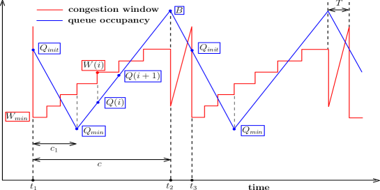
Figure 11: Evolution of TCP congestion window and bottleneck queue occupancy for heterogeneous traffic flows involving TCP and CBR streams.

We begin by analyzing the queue occupancy evolution in the congestion avoidance phase (Section 9.1.1), and subsequently move to the fast retransmit, fast recovery phase (Section 9.1.2).

9.1.1   Congestion Avoidance

In this section, we analyze in detail the queue dynamics in the congestion avoidance phase ($t_{1}$ to $t_{2}$ in Figure 11). Unlike the congestion avoidance in the single TCP source case (depicted in Figure 3a), where the queue occupancy varies monotonically, this phase in the TCP-CBR case can be split into the following two regions:

1. increasing region: queue occupancy builds up from $Q_{min}\text{ to }B$ over $c-c_{1}$ slots,

2. decreasing region: queue occupancy reduces from $Q_{init}\text{ to }Q_{min}$ over $c_{1}$ slots.

We seek to obtain the relationships between queue occupancy at various stages in each of the above mentioned regions.

Increasing region: Let $RTT(i)$ denote the duration of the $i$^th slot. Recall that $RTT(i)$ is the RTT encountered by the probing packet transmitted in the $i$^th slot. Therefore, we can write

$$RTT(i)=2\tau+\frac{Q(i)}{\mu},$$ (15)

where $2\tau$ is the round trip propagation delay, and the second term is the queueing delay faced by the probing packet at the ingress of the bottleneck link. Note that $Q(i)$ is the queue occupancy at the onset of $i$^th slot, which is exactly the queue occupancy seen by the probing packet.

We know that the TCP source injects an amount of traffic equal to $W(i)S_{tcp}$ over $i$^th slot. Let $D_{T}(i)$ denote the amount of TCP traffic drained from the queue during $i$^th slot. Recall that the TCP source transmits an additional packet in each slot relative to the previous slot. Based on the analysis in [Sun et al. (2004)], we make a reasonable assumption that the TCP component of queue occupancy builds up at the rate of 1 packet per slot. Relating initial states of the queue, input, and output during $i$^th and $(i+1)$^th slots, we obtain the following equation for the TCP component of the queue.

$$[Q_{T}(i+1)+W(i+1)S_{tcp}-D_{T}(i+1)]-[Q_{T}(i)+W(i)S_{tcp}-D_{T}(i)]=S_{tcp},\forall i\in[c_{1}+1,c-1].$$ (16)

Here, the first and the second terms in LHS signify the queue occupancy at end of $(i+1)$^th and $i$^th slots, respectively.

We now derive an analogous equation for CBR component of the queue. The amount of traffic injected by the CBR stream during the $i$^th slot is given by $RTT(i)R$. Note that in the increasing region $RTT(i+1)>RTT(i)$, and hence the CBR source transmits higher amount of traffic in the $(i+i)$^th slot relative to the $i$^th slot. Let $\Delta Q_{C}(i)$ denote the difference in the CBR component of the queue at the end of $(i+1)$^th and $i$^th slots. Let $D_{C}(i)$ denote the amount of CBR traffic drained from the queue during $i$^th slot. Relating the initial queue states, input and output during $i$^th and $(i+1)$^th slots, we obtain the following equation for the CBR component of the queue.

$$\begin{split}[Q_{C}(i+1)+RTT(i+1)R-D_{C}(i+1)]-[Q_{C}(i)+RTT(i)R-D_{C}(i)]=\Delta Q_{C}(i),\\ \forall i\in[c_{1}+1,c-1].\end{split}$$ (17)

We know that $Q_{T}(i)+Q_{C}(i)=Q(i)$, and the total queue drain over the $i$^th slot $D_{T}(i)~{}+~{}D_{C}(i)~{}=~{}\mu RTT(i)$. Using these relationships in Equations (16) and (17), and subsequently adding them up, we obtain

$$\begin{split}Q(i+1)-Q(i)+(R-\mu)[RTT(i+1)-RTT(i)]+[W(i+1)-W(i)]S_{tcp}\\ =S_{tcp}+\Delta Q_{C}(i),\forall i\in[c_{1}+1,c-1].\end{split}$$ (18)

We know that $Q_{T}(i+1)-Q_{T}(i)=S_{tcp},\forall i\in[c_{1}+1,c-1]$, and $W(i+1)-W(i)=1$. Hence, the queue occupancy increases at the rate of $\Delta Q_{C}(i)+S_{tcp}$ per slot i.e., $Q(i+1)-Q(i)=S_{tcp}+\Delta Q_{C}(i),\forall i\in[c_{1}+1,c-1]$. Using these relationships in Equations (15) and (18), we obtain

$$\Delta Q_{C}(i)=\frac{RS_{tcp}}{\mu-R},\forall i\in[c_{1}+1,c-1].$$ (19)

This suggests that in the increasing region of congestion avoidance, the CBR traffic builds up in the queue at a constant rate of $\frac{RS_{tcp}}{\mu-R}$ per slot. Further, the ratio of increments in CBR and TCP components per slot equals $\frac{R}{\mu-R}$. Interestingly, this ratio is independent of TCP parameters.

We now seek to derive the relationship between the end-to-end queue occupancy in the increasing region (i.e., $Q_{min}$ and $B$). From Equation (19) we can calculate that $Q(i)$ increases at the rate of $\frac{\mu S_{tcp}}{\mu-R}$ per slot. Since the queue occupancy build up from $Q_{min}$ to $B$ comprises of $c-c_{1}$ slots, we can write

$$Q_{min}+(c-c_{1})\frac{\mu S_{tcp}}{\mu-R}=B.$$ (20)

Decreasing region: We now move to the decreasing region of the congestion avoidance, i.e. $i\in[1,c_{1}]$. Note that since the queue occupancy is a decreasing function of $i$ in this region, we can infer (from Equation (15)) that RTTs encountered by the probing packets in successive slots reduce progressively. Using the basic input-output equation in each of the slots, we can write

$$Q(i+1)=Q(i)+RTT(i)R+W(i)S_{tcp}-\mu RTT(i),\forall i\in[1,c_{1}].$$ (21)

By definition, $Q(1)=Q_{init}$, $Q(c_{1}+1)=Q_{min}$, and $W(i)=W_{min}+i-1$. Adding up the $c_{1}$ components of Equation (21), we obtain the following relationship between $Q_{init}$ and $Q_{min}$.

$$\begin{split}Q_{min}=Q_{init}+(R-\mu)\sum\limits_{i=1}^{c_{1}}RTT(i)+\sum\limits_{i=1}^{c_{1}}(W_{min}+i-1)S_{tcp}.\end{split}$$ (22)

Substituting Equation (15) in (22), we obtain

$$Q_{min}=Q_{init}\alpha^{c_{1}}+\Bigg{(}\frac{1-\alpha^{c_{1}}}{1-\alpha}\Bigg{)}[W_{min}S_{tcp}-(1-\alpha)2\mu\tau]+S_{tcp}\sum_{j=0}^{c_{1}-2}(c_{1}-1-j)\alpha^{j},$$ (23)

where $\alpha=R/\mu$.

9.1.2   Fast Retransmit, Fast Recovery

We now move to modeling the queue dynamics in the fast retransmit, fast recovery phase (interval between $t_{2}$ and $t_{3}$ in Figure 11).

End-to-end queue occupancy: It can be shown that over the duration $T$, the TCP NewReno source transmits $W_{min}$ packets and receives $2W_{min}$ ACKs (including duplicates). A total of $2W_{min}$ ACK arrivals imply that $2W_{min}$ TCP packets have escaped the bottleneck link in the duration $T$. Recall (from Section 2.1) that there are $2W_{min}$ outstanding packets at the start of the fast retransmit, fast recovery phase (at $t_{2}$ in Figure 11). This implies that the fast retransmit, fast recovery phase ends (at $t_{3}$) exactly when all of the TCP packets that were outstanding at the beginning (at $t_{2}$) have been acknowledged. We already know that at $t_{2}$ the queue occupancy $B$ is shared between CBR and TCP traffic in the ratio $\frac{R}{\mu-R}$. This implies that over the duration of $T$, along with $2W_{min}S_{tcp}$ bytes of TCP data, $2W_{min}S_{tcp}\frac{R}{\mu-R}$ bytes of CBR data have also escaped the bottleneck link. Therefore, we obtain the expression for $T$ as

$$T=\frac{2W_{min}S_{tcp}+2W_{min}S_{tcp}\frac{R}{\mu-R}}{\mu}=\frac{2W_{min}S_{tcp}}{\mu-R}$$ (24)

Owing to the transmission of $W_{min}$ TCP packets, we can express the relationship between $B$ and $Q_{init}$

$$Q_{init}=B+(R-\mu)T+W_{min}S_{tcp}$$ (25)

From Equations (24) and (25), we obtain

$$Q_{init}=B-W_{min}S_{tcp}$$ (26)

TCP component of queue at the end: We now seek to compute the amount of TCP data present in the queue at $t_{3}$. As discussed previously, all the TCP packets that are outstanding at $t_{2}$ are acknowledged at $t_{3}$. This clearance of backlog implies that all of the TCP packets present in the queue at $t_{3}$ must have been injected in the interval $T$ (between $t_{2}$ and $t_{3}$). At $t_{3}$, these packets are either present in the queue or are in flight in the channel. For the ease of analysis, we make a reasonable assumption that the ratio of amount of TCP data present in the queue at $t_{3}$ and total TCP data injected in $T$ is comparable to the corresponding ratio of the CBR stream. Recall that the amount of CBR and TCP data transmitted in the interval $T$ are given as $RT$ and $W_{min}S_{tcp}$, respectively. Hence, the ratio of CBR and TCP data in the queue at $t_{3}$ can be written as $\frac{RT}{W_{min}S_{tcp}}$. Using the expression for $T$ from Equation (24), this ratio reduces to $\frac{2R}{\mu-R}$.

This finding is striking as the ratio of CBR and TCP components in the queue doubles during the interval $T$. Recall that this ratio is equal to $\frac{R}{\mu-R}$ at the beginning of this interval. The justification for the increase in the ratio is the following: As per the TCP NewReno protocol design, after the retransmission of the lost packet, the TCP source makes no transmissions until it receives $W_{min}$ ACKs. On the contrary, the CBR source continues to pump in data at the steady rate of $R$. Thus, the queue is predominantly occupied by the CBR traffic at the end of $T$, thereby bloating the ratio of CBR and TCP contents in the queue.

Using this ratio, the amount of TCP data in the queue at $t_{3}$ can be expressed as $Q_{init}(\frac{\mu-R}{\mu+R})$. Naturally, the channel will be shared between the TCP and the CBR streams in the same proportion as the queue. Hence, the amount of in-flight TCP data can be approximated as $2\mu\tau(\frac{\mu-R}{\mu+R})$. Therefore, we obtain an equation for the TCP component of $Q_{init}$ as follows.

$$Q_{init}\Big{(}\frac{\mu-R}{\mu+R}\Big{)}=W_{min}S_{tcp}-2\mu\tau\Big{(}\frac{\mu-R}{\mu+R}\Big{)}$$ (27)

9.1.3   Congestion Window

We now move to relating the congestion windows at the start and the end of a cycle. As discussed in Section 2.1, at the beginning of a cycle $W$ is set to half its value at the end of congestion avoidance in the previous cycle. Recall that $W$ is incremented $c-1$ times during congestion avoidance. Relating the congestion window at the start and the end of congestion avoidance, we obtain

$$W_{min}=\frac{W_{min}+c-1}{2}$$

which on simplification gives

$$W_{min}=c-1$$ (28)

Solving the simultaneous equations (26), (27) and (28), we obtain the closed form expressions for $W_{min}$, $Q_{init}$ and $c$ as follows.

$$W_{min}=\frac{(B+2\mu\tau)(1-\alpha)}{2S_{tcp}}$$ (29)

$$Q_{init}=\frac{(B+2\mu\tau)(1+\alpha)}{2}-2\mu\tau$$ (30)

$$c=\frac{(B+2\mu\tau)(1-\alpha)}{2S_{tcp}}+1$$ (31)

Using these in Equations (20) and (22), we obtain

$$Q_{min}+\Big{[}\frac{(B+2\mu\tau)(1-\alpha)}{2S_{tcp}}-c_{1}+1\Big{]}\Big{[}\frac{S_{tcp}}{1-\alpha}\Big{]}=B$$ (32)

$$Q_{min}=\Big{[}\frac{(B+2\mu\tau)(1+\alpha)}{2}-2\mu\tau\Big{]}\alpha^{c_{1}}+\Big{[}\frac{(B-2\mu\tau)(1-\alpha^{c_{1}})}{2}\Big{]}+S_{tcp}\sum_{j=0}^{c_{1}-2}(c_{1}-1-j)\alpha^{j}$$ (33)

This completes the formal derivation of Equation (5) that we briefly described in Section 2.2.1.

9.2 Characterization of CBR Jitter

In this section, we present the detailed derivation of analytical expression for $m_{tcp}$ – the maximum number of TCP packets transmitted between two successive CBR packets.

As pointed out in Section 9.1.2, during congestion avoidance, the queue and hence the channel are shared by the CBR and TCP streams in the ratio $\frac{R}{\mu-R}$ (see Equation (19)). In other words, the TCP stream gets served at the rate of $\mu-R$. Let us now consider two adjacent ACKs, none corresponding to probing packets. The time spacing between the two ACKs can be given as $\frac{nS_{tcp}}{\mu-R}$, since there are $n$ packet receptions between the transmission of two ACKs. Note that each of these ACKs give rise to transmission of an $n-$packet burst.

On the other hand, the transmission of a probing packet gives rise to a slightly different situation. Recall that the probing packet is always transmitted as a part of an $(n+1)-$packet burst. When the earliest packet in this burst arrives at the receiver, two scenarios can occur depending on $p$ - the number of packets waiting at the receiver to be acknowledged. Naturally, $p\leq n-1$. We now consider the different possible values that $p$ can take, and analyze each scenario.

1. $p<n-1$: In this case, the reception of the earliest $n-p$ packets trigger an ACK. The remaining $p+1$ packets in the burst wait for the earliest $n-p-1$ packets from the subsequent burst for triggering the next ACK. In this case, the time interval between these two ACKs can be calculated to be $\frac{nS_{tcp}}{\mu-R}$.

2. $p=n-1$: In this case, the reception of the first packet in the burst triggers an ACK. The latter $n$ packets of the same burst trigger another ACK. It is worth remarking that since the TCP packet transmissions are bursty in nature, it is fairly reasonable to assume that the TCP packets belonging to a burst occupy contiguous locations in the queue. Hence, the TCP packets consume the full channel capacity ($\mu$) until the burst is served by the queue. Therefore, the time interval between the two back-to-back ACKs in this case can be calculated as $\frac{nS_{tcp}}{\mu}$.

The important difference between the above two scenarios is the following: For generating two ACKs, in the latter case a single burst of packets is sufficient, whereas in the former case two bursts need to be necessarily transmitted. Therefore, the ACKs are spaced more closely in the latter case than the former. Hence, the ACKs corresponding to the latter case give rise to maximum number TCP packets injected between two CBR packets. It can be shown that the situation $p=n-1$ is guaranteed to occur once every $n$^th window update during congestion avoidance. Hence, for this analysis we restrict our attention to the latter case.

We refer back to Figure 4 for the current analysis. If $T_{h}<\frac{nS_{tcp}}{\mu}$, then $m_{tcp}=n+1$ as no more than one burst can be transmitted in the interval $T_{h}$. On the other hand, if $T_{h}>\frac{nS_{tcp}}{\mu}$, the number of $n-$packet bursts transmitted in addition to the $(n+1)-$packet burst in the interval $T_{h}$ can be expressed as $1+\left\lfloor\frac{T_{h}-\frac{nS_{tcp}}{\mu}}{\frac{nS_{tcp}}{\mu-R}}\right\rfloor$. Hence, we write the general expression for $m_{tcp}$ as

$$m_{tcp}=n+1+\Bigg{(}1+\left\lfloor\frac{T_{h}-\frac{nS_{tcp}}{\mu}}{\frac{nS_{tcp}}{\mu-R}}\right\rfloor\Bigg{)}nI_{\big{(}T_{h}>\frac{nS_{tcp}}{\mu}\big{)}}.$$ (34)

References

- [1]
- Aad et al. (2008) Imad Aad, Jean-Pierre Hubaux, and Edward W Knightly. 2008. Impact of denial of service attacks on ad hoc networks. IEEE/ACM transactions on networking 16, 4 (2008), 791–802.
- Al Osman et al. (2007) H Al Osman, M Eid, R Iglesias, and A El Saddik. 2007. Alphan: Application layer protocol for haptic networking. In Haptic, Audio and Visual Environments and Games, 2007. HAVE 2007. IEEE International Workshop on. IEEE, 96–101.
- Andreadis et al. (2008) Alessandro Andreadis, Giuliano Benelli, and Riccardo Zambon. 2008. An admission control algorithm for QoS provisioning in IEEE 802.11 e EDCA. In Wireless Pervasive Computing, 2008. ISWPC 2008. 3rd International Symposium on. IEEE, 298–302.
- Arranz et al. (2001) MG Arranz, R Aguero, L Munoz, and P Mahonen. 2001. Behavior of UDP-based applications over IEEE 802.11 wireless networks. In Personal, Indoor and Mobile Radio Communications, 2001 12th IEEE International Symposium on, Vol. 2. IEEE, F–F.
- Bai and Yan (2012) Botao Bai and Jinyao Yan. 2012. The role of buffer unit in routers with very small buffers. In Computing and Networking Technology (ICCNT), 2012 8th International Conference on. IEEE, 1–4.
- Beritelli et al. (2003) Francesco Beritelli, Giuseppe Ruggeri, and Giovanni Schembra. 2003. TCP-friendly transmission of voice over IP. Transactions on Emerging Telecommunications Technologies 14, 3 (2003), 193–203.
- Bhardwaj et al. (2013) Amit Bhardwaj, Onkar Dabeer, and Subhasis Chaudhuri. 2013. Can we improve over weber sampling of haptic signals?. In Information Theory and Applications Workshop (ITA), 2013. IEEE, 1–6.
- Boggia et al. (2007) Gennaro Boggia, Pietro Camarda, Luigi Alfredo Grieco, and Saverio Mascolo. 2007. Feedback-based control for providing real-time services with the 802.11 e MAC. IEEE/ACM transactions on networking 15, 2 (2007), 323–333.
- Bonald et al. (2000) Thomas Bonald, Martin May, and J-C Bolot. 2000. Analytic evaluation of RED performance. In INFOCOM 2000. Nineteenth Annual Joint Conference of the IEEE Computer and Communications Societies. Proceedings. IEEE, Vol. 3. IEEE, 1415–1424.
- Bruno et al. (2008) Raffaele Bruno, Marco Conti, and Enrico Gregori. 2008. Throughput analysis and measurements in IEEE 802.11 WLANs with TCP and UDP traffic flows. IEEE Transactions on Mobile Computing 7, 2 (2008), 171–186.
- Bu et al. (2006) Tian Bu, Yong Liub, and Don Towsley. 2006. On the TCP-Friendliness of VoIP Traffic. In IEEE INFOCOM. 1.
- Carlucci et al. (2014) Gaetano Carlucci, Luca De Cicco, and Saverio Mascolo. 2014. Modelling and control for web real-time communication. In Decision and Control (CDC), 2014 IEEE 53rd Annual Conference on. IEEE, 6824–6829.
- Chen et al. (2006) Xiang Chen, Hongqiang Zhai, Xuejun Tian, and Yuguang Fang. 2006. Supporting QoS in IEEE 802.11 e wireless LANs. IEEE Transactions on Wireless Communications 5, 8 (2006), 2217–2227.
- Cheng et al. (2008) Xiaolin Cheng, Prasant Mohapatra, Sung-Ju Lee, and Sujata Banerjee. 2008. Performance evaluation of video streaming in multihop wireless mesh networks. In Proceedings of the 18th International Workshop on Network and Operating Systems Support for Digital Audio and Video. ACM, 57–62.
- Cizmeci et al. (2014) Burak Cizmeci, Rahul Chaudhari, Xiao Xu, Nicolas Alt, and Eckehard Steinbach. 2014. A Visual-Haptic Multiplexing Scheme for Teleoperation over Constant-Bitrate Communication Links. In Haptics: Neuroscience, Devices, Modeling, and Applications. Springer, 131–138.
- Clarke et al. (2006) Stella Clarke, Gerhard Schillhuber, Michael F Zaeh, and Heinz Ulbrich. 2006. Telepresence across delayed networks: a combined prediction and compression approach. In Haptic Audio Visual Environments and their Applications, 2006. HAVE 2006. IEEE International Workshop on. IEEE, 171–175.
- Daniel et al. (2003) Edward J Daniel, Christopher M White, and Keith A Teague. 2003. An interarrival delay jitter model using multistructure network delay characteristics for packet networks. In Signals, Systems and Computers, 2004. Conference Record of the Thirty-Seventh Asilomar Conference on, Vol. 2. IEEE, 1738–1742.
- De Cicco et al. (2013) Luca De Cicco, Gaetano Carlucci, and Saverio Mascolo. 2013. Experimental investigation of the google congestion control for real-time flows. In Proceedings of the 2013 ACM SIGCOMM workshop on Future human-centric multimedia networking. ACM, 21–26.
- De Cicco et al. (2011) Luca De Cicco, Saverio Mascolo, and Vittorio Palmisano. 2011. Skype video congestion control: An experimental investigation. Computer Networks 55, 3 (2011), 558–571.
- Doshi and Cao (2003) Rushabh Doshi and Pei Cao. 2003. Streaming traffic fairness over low bandwidth WAN links. In Internet Applications. WIAPP 2003. Proceedings. The Third IEEE Workshop on. IEEE, 30–34.
- Eid et al. (2011) Mohamad Eid, Jongeun Cha, and Abdulmotaleb El Saddik. 2011. Admux: An adaptive multiplexer for haptic–audio–visual data communication. IEEE Transactions on Instrumentation and Measurement 60, 1 (2011), 21–31.
- Festo (2013) Festo. 2013. Festo ExoHand: http://www.festo.com/. (2013).
- Floyd et al. (2004) Sally Floyd, Andrei Gurtov, and Tom Henderson. 2004. The NewReno modification to TCP’s fast recovery algorithm. (2004).
- Fujimoto and Ishibashi (2005) Masaki Fujimoto and Yutaka Ishibashi. 2005. Packetization interval of haptic media in networked virtual environments. In Proceedings of 4th ACM SIGCOMM workshop on Network and system support for games. ACM, 1–6.
- Gokhale et al. (2015) Vineet Gokhale, Subhasis Chaudhuri, and Onkar Dabeer. 2015. HoIP: A point-to-point haptic data communication protocol and its evaluation. In Twenty First National Conference on Communications (NCC). IEEE, 1–6.
- Gokhale et al. (2016) Vineet Gokhale, Jayakrishnan Nair, and Subhasis Chaudhuri. 2016. Opportunistic adaptive haptic sampling on forward channel in telehaptic communication. In Haptics Symposium (HAPTICS). IEEE.
- Gokhale et al. (2017) Vineet Gokhale, Jayakrishnan Nair, and Subhasis Chaudhuri. 2017. Congestion Control for Network-Aware Telehaptic Communication. ACM Transactions on Multimedia Computing, Communications, and Applications (TOMM) 13, 2 (2017), 17.
- Gupta et al. (2002) Vikram Gupta, Srikanth Krishnamurthy, and Michalis Faloutsos. 2002. Denial of service attacks at the MAC layer in wireless ad hoc networks. In MILCOM 2002. Proceedings, Vol. 2. IEEE, 1118–1123.
- Gupta et al. (2004) Vikram Gupta, Srikanth V Krishnamurthy, and Michalis Faloutsos. 2004. Improving the performance of TCP in the presence of interacting UDP flows in ad hoc networks. In International Conference on Research in Networking. Springer, 64–75.
- Handley et al. (2002) Mark Handley, Sally Floyd, Jitendra Padhye, and Jörg Widmer. 2002. TCP friendly rate control (TFRC): Protocol specification. Technical Report.
- Haßlinger and Hohlfeld (2008) Gerhard Haßlinger and Oliver Hohlfeld. 2008. The Gilbert-Elliott model for packet loss in real time services on the Internet. In Measuring, Modelling and Evaluation of Computer and Communication Systems (MMB), 2008 14th GI/ITG Conference-. VDE, 1–15.
- He and Chan (2003) Jingyi He and S-HG Chan. 2003. TCP and UDP performance for Internet over optical packet-switched networks. In Communications, 2003. ICC’03. IEEE International Conference on, Vol. 2. IEEE, 1350–1354.
- Hinterseer et al. (2008) Peter Hinterseer, Sandra Hirche, Subhasis Chaudhuri, Eckehard Steinbach, and Martin Buss. 2008. Perception-based data reduction and transmission of haptic data in telepresence and teleaction systems. IEEE Transactions on Signal Processing 56, 2 (2008), 588–597.
- Immersion (2003) Immersion. 2003. CyberGrasp User’s Guide v1.2. (2003).
- Karam and Tobagi (2002) Mansour J Karam and Fouad A Tobagi. 2002. Analysis of delay and delay jitter of voice traffic in the Internet. Computer Networks 40, 6 (2002), 711–726.
- Kim et al. (2009) Sunmyeng Kim, Rongsheng Huang, and Yuguang Fang. 2009. Deterministic priority channel access scheme for QoS support in IEEE 802.11 e wireless LANs. IEEE Transactions on Vehicular Technology 58, 2 (2009), 855–864.
- Knoche and De Meer (1997) H Knoche and H De Meer. 1997. QoS parameters: A comparative study. Univ. Hamburg, Hamburg, Germany, Tech. Rep (1997).
- Lin and Lai (2007) Y-C Lin and Wei Kuang Lai. 2007. Adaptive bandwidth sharing mechanism for quality of service administration in infrastructure wireless networks. IET communications 1, 5 (2007), 846–857.
- Marshall et al. (2008) Alan Marshall, Kian Meng Yap, and Wai Yu. 2008. Providing QoS for networked peers in distributed haptic virtual environments. Advances in Multimedia (2008).
- Nasir and Khalil (2012) Qassim Nasir and Enas Khalil. 2012. Perception based adaptive haptic communication protocol (pahcp). In Computer Systems and Industrial Informatics (ICCSII), 2012 International Conference on. IEEE, 1–6.
- Papadimitriou and Tsaoussidis (2006) Panagiotis Papadimitriou and Vassilis Tsaoussidis. 2006. On transport layer mechanisms for real-time QoS. J. Mobile Multimedia 1, 4 (2006), 342–363.
- Rejaie et al. (1999) Reza Rejaie, Mark Handley, and Deborah Estrin. 1999. RAP: An end-to-end rate-based congestion control mechanism for realtime streams in the Internet. In INFOCOM’99. Eighteenth Annual Joint Conference of the IEEE Computer and Communications Societies. Proceedings. IEEE, Vol. 3. IEEE, 1337–1345.
- Rhee et al. (2000) Injong Rhee, Volkan Ozdemir, and Yung Yi. 2000. TEAR: TCP emulation at receivers-flow control for multimedia streaming. Technical Report. NCSU Technical Report.
- Rohner et al. (2005) Christian Rohner, Erik Nordström, Per Gunningberg, and Christian Tschudin. 2005. Interactions between TCP, UDP and routing protocols in wireless multi-hop ad hoc networks. In Proc. IEEE ICPS Workshop on Multi-hop Ad hoc Networks: from theory to reality (REALMAN’05).
- Ryu et al. (2003) Seungwan Ryu, Christopher Rump, and Chunming Qiao. 2003. Advances in internet congestion control. IEEE Communications Surveys & Tutorials 5, 1 (2003), 28–39.
- Sakr et al. (2011) Nizar Sakr, Nicolas D Georganas, and Jiying Zhao. 2011. Human perception-based data reduction for haptic communication in six-dof telepresence systems. IEEE Transactions on Instrumentation and Measurement 60, 11 (2011), 3534–3546.
- Sawashima et al. (1997) Hidenari Sawashima, Yoshiaki Hori, Hideki Sunahara, and Yuji Oie. 1997. Characteristics of UDP packet loss: Effect of tcp traffic. In Proceedings of INET’97: The Seventh Annual Conference of the Internet Society.
- Sensable (2012) Sensable. 2012. Phantom omni device reference: www.sensable.com/haptic-phantom-omni.htm. (july 2012).
- Shetiya and Sharma (2005) Harish Shetiya and Vinod Sharma. 2005. Algorithms for routing and centralized scheduling to provide QoS in IEEE 802.16 mesh networks. In Proceedings of the 1st ACM workshop on Wireless multimedia networking and performance modeling. ACM, 140–149.
- Steinbach et al. (2011) Eckehard Steinbach, Sandra Hirche, Julius Kammerl, Iason Vittorias, and Rahul Chaudhari. 2011. Haptic data compression and communication. IEEE Signal Processing Magazine 28, 1 (2011), 87–96.
- Sun et al. (2004) Jinsheng Sun, Moshe Zukerman, King-Tim Ko, Guanrong Chen, and Sammy Chan. 2004. Effect of large buffers on TCP queueing behavior. In INFOCOM 2004. Twenty-third AnnualJoint Conference of the IEEE Computer and Communications Societies, Vol. 2. IEEE, 751–761.
- Suznjevic et al. (2014) Mirko Suznjevic, Jose Saldana, Maja Matijasevic, Julián Fernández-Navajas, and José Ruiz-Mas. 2014. Analyzing the effect of TCP and server population on massively multiplayer games. International Journal of Computer Games Technology 2014 (2014), 2.
- Tirumala (1999) Ajay Tirumala. 1999. Iperf: The TCP/UDP bandwidth measurement tool. http://dast. nlanr. net/Projects/Iperf/ (1999).
- Veres et al. (2001) Andras Veres, Andrew T. Campbell, Michael Barry, and Li-Hsiang Sun. 2001. Supporting service differentiation in wireless packet networks using distributed control. IEEE Journal on selected Areas in Communications 19, 10 (2001), 2081–2093.
- Villamizar and Song (1994) Curtis Villamizar and Cheng Song. 1994. High performance TCP in ANSNET. ACM SIGCOMM Computer Communication Review 24, 5 (1994), 45–60.
- Vishwanath et al. (2011) Arun Vishwanath, Vijay Sivaraman, and George N Rouskas. 2011. Anomalous loss performance for mixed real-time and TCP traffic in routers with very small buffers. IEEE/ACM Transactions on Networking 19, 4 (2011), 933–946.
- Wirz et al. (2008) Raul Wirz, Manuel Ferre, Raul Marín, Jorge Barrio, José M Claver, and Javier Ortego. 2008. Efficient transport protocol for networked haptics applications. In Haptics: Perception, Devices and Scenarios. Springer, 3–12.
- Wong and Donaldson (2003) George W Wong and Robert W Donaldson. 2003. Improving the QoS performance of EDCF in IEEE 802.11 e wireless LANs. In Communications, Computers and signal Processing, 2003. PACRIM. 2003 IEEE Pacific Rim Conference on, Vol. 1. IEEE, 392–396.
- Xu et al. (2012) Yang Xu, Chenguang Yu, Jingjiang Li, and Yong Liu. 2012. Video telephony for end-consumers: measurement study of Google+, iChat, and Skype. In Proceedings of the 2012 Internet Measurement Conference. ACM, 371–384.
- Xylomenos and Polyzos (1999) George Xylomenos and George C Polyzos. 1999. TCP and UDP performance over a wireless LAN. In INFOCOM’99. Eighteenth Annual Joint Conference of the IEEE Computer and Communications Societies. Proceedings. IEEE, Vol. 2. IEEE, 439–446.
- Yao et al. (2002) Shun Yao, Fei Xue, Biswanath Mukherjee, SJ Ben Yoo, and Sudhir Dixit. 2002. Electrical ingress buffering and traffic aggregation for optical packet switching and their effect on TCP-level performance in optical mesh networks. IEEE Communications Magazine 40, 9 (2002), 66–72.
- Zahedi and Pahlavan (2000) Ali Zahedi and Kevin Pahlavan. 2000. Capacity of a wireless LAN with voice and data services. IEEE Transactions on Communications 48, 7 (2000), 1160–1170.
- Zhai et al. (2006) Hongqiang Zhai, Jianfeng Wang, and Yuguang Fang. 2006. Providing statistical QoS guarantee for voice over IP in the IEEE 802.11 wireless LANs. IEEE Wireless Communications 13, 1 (2006), 36–43.
- Zhang et al. (2013) Xinggong Zhang, Yang Xu, Hao Hu, Yong Liu, Zongming Guo, and Yao Wang. 2013. Modeling and analysis of Skype video calls: Rate control and video quality. IEEE Transactions on Multimedia 15, 6 (2013), 1446–1457.