Technical design and commissioning of a sensor net for fine-meshed measuring of the magnetic field at the KATRIN spectrometer

Abstract

The KArlsruhe TRItium Neutrino experiment (KATRIN) aims to measure the absolute neutrino mass scale with an unprecedented sensitivity of 0.2 eV/c² (90% C.L.), using $\beta$ decay electrons from tritium decay. The kinetic energy of the decay electrons is measured using an electrostatic integrating main spectrometer with magnetic adiabatic collimation and requires a certain magnetic field profile. For the control of the magnetic field in the main spectrometer area two networks of mobile magnetic field sensor units are developed and commissioned. The radial system is operated close to the outer surface of the main spectrometer whereas the vertical one is mounted along vertical planes left and right of the main spectrometer. The sensor setup can take several thousand magnetic field samples at a fine meshed grid, thus allowing to study the magnetic field inside the main spectrometer and the influence of magnetic materials in the vicinity of the main spectrometer.

magnetic field sensor net, Mobile Magnetic Sensor Unit, KATRIN, Spectrometer

1 Introduction

The Karlsruhe TRItium Neutrino experiment [1] is a next-generation experiment for a direct and model-independent determination of the absolute neutrino mass scale. By analyzing the shape of the tritium $\beta$-decay spectrum near the endpoint energy at $E_{0}=18.6$ KATRIN will achieve a sensitivity of $m_{v}=0.2$ eV/c² (90% C.L.). A schematic overview of the KATRIN setup is shown in fig:KATRINsetup.

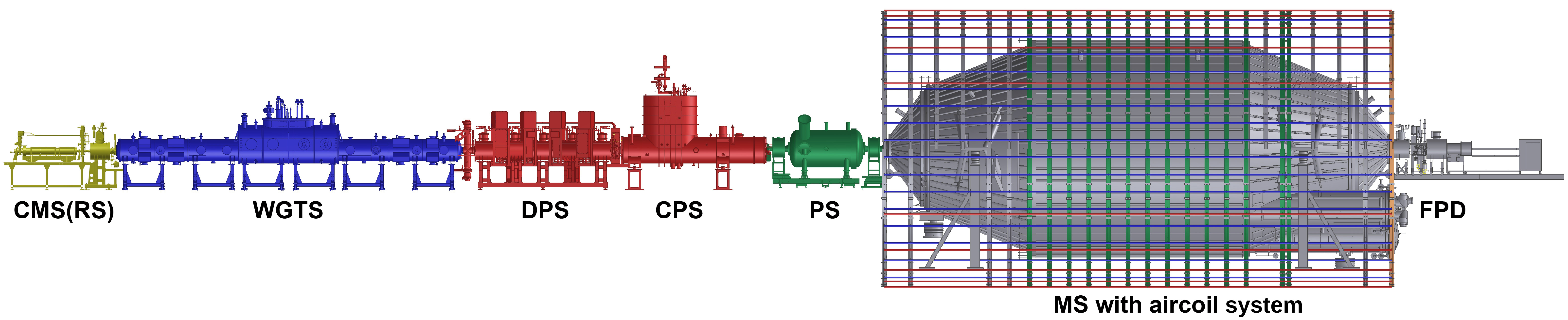
Figure 1: Schematic overview of 70m long KATRIN setup, consisting of calibration and monitor rear system (CMS/RS), the electron emitting section with the windowless gaseous tritium source (WGTS), differential pumping (DPS) and cryotrapping section (CPS), the small pre-spectrometer (PS) and the large main spectrometer (MS) with the aircoil system and lastly the segmented PIN-diode detector with upstream pinch and detector magnet (FPD).

The experimental setup uses a magnetic transport flux of 190 Tcm² to guide the $\beta$-decay electrons from a windowless gaseous tritium source through a pumping section towards two electrostatic energy spectrometers and onto a detector. The operating principle of the spectrometers is based on a magnetic adiabatic collimation with electrostatic filtering (MAC-E filter)[2, 3, 4], where a retarding electric potential is used to reflect electrons below a given energy threshold. In order to ensure the correct function of the MAC-E filter, a certain magnetic field profile is required. The shape of the magnetic flux tube inside the main spectrometer (MS) has a significant influence on the overall energy resolution function of the spectrometer. In addition, the alignment and shape of the magnetic field lines plays an essential role for the electronic background via a) the generation of secondary electrons through wall contact of energetic electrons (see fig:MagLinesKAT) and b) the generation and storage of charged particles due to penning traps and the magnetic bottle effect.

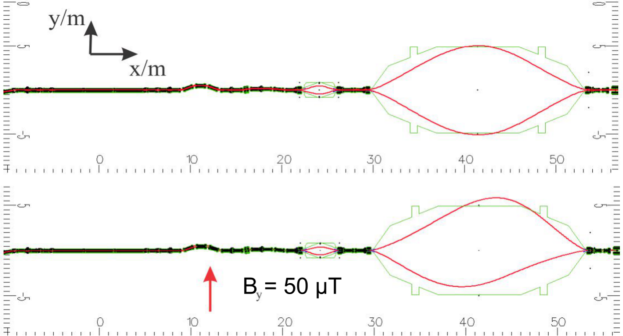
Figure 2: A CAD view (taken from a PartOpt [6] simulation) showing the KATRIN high field solenoids energized according to reference values, and in red the corresponding boundary $190$ Tcm² magnetic transport flux lines in the central horizontal plane without air coils. Both axes are given in meters. Top: without external perturbation touching the spectrometer walls. Bottom: In case of an additional global external magnetic field (e.g.earth magnetic field) of $By=50$ $\mu$T the perturbed field lines intersect with the MS walls.

For the control of the desired magnetic field shape, large aircoil systems [15, 8] are arranged around the MS: The earth magnetic field compensation system (EMCS) for the compensation of the earth magnetic field and the low field coil system (LFCS) for the fine tuning of the magnetic transport flux tube (see fig:Aircoilsystem). The requirements on the magentic field and achieved performances of the magnetic field generating systems are described in more detail in [5]. Although the calculation of the magnetic field inside the main spectrometer generated by all the relevant current leading elements is in principle possible and well performed, perturbing external dipoles, magnetization effects in the direct environment of the spectrometer and the incorrect alignment and orientation of the spectrometer solenoids, EMCS and LFCS can have a disturbing influence. Due to the extreme vacuum conditions the installation of magnetic field sensors inside the main spectrometer is not possible during KATRIN operation.

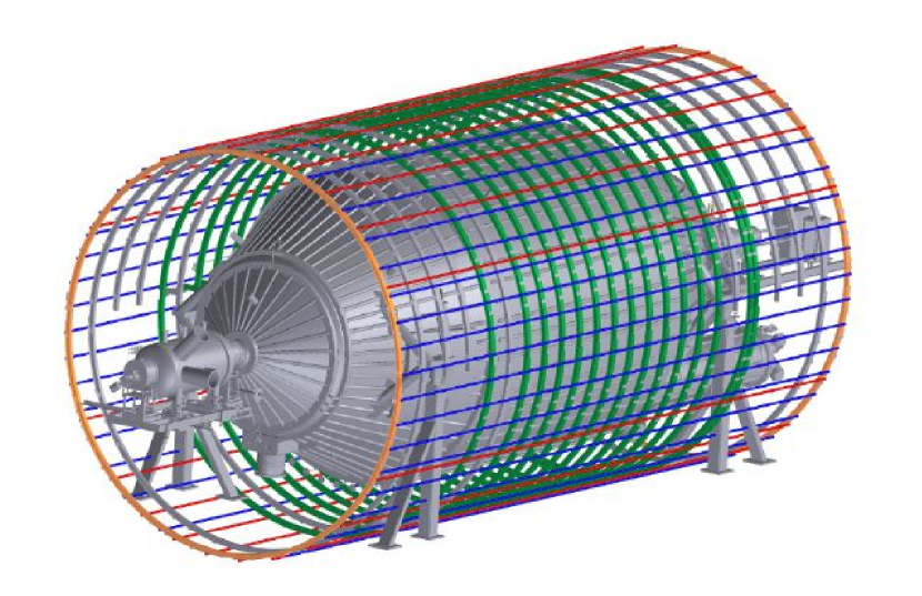
(a)

(b)

Figure 3: The CAD (a) and photographic (b) view of KATRIN main spectrometer. LFCS: The ring shaped low field coils distributed co-axially along the MS (green circles in Figure (a)). The current leading elements of the EMCS run parallel to the spectrometer walls (blue and red lines as well as orange circles in Figure (a)). A more detailed description can be found in [8].

This paper focuses on the technical realization of two magnetic sensor networks that allow to measure the magnetic field in the direct environment of KATRIN main spectrometer over large areas with fine meshed sample positions. The radial magnetic measuring system (RMMS), based on the mobile sensor unit [10], is operated on 4 LFCS rings. The vertical magnetic measuring system (VMMS) covers vertical planes parallel to the MS beam axis.

2 The radial magnetic field measuring system

The radial magnetic field measuring system (RMMS) is a system for measuring the magnetic field close to the KATRIN MS surface. The initial concept is based on a mobile sensor unit (MobSU) [10], which moves on the inner side of the LFCS support ring and measures the magnetic field on predefined sampling positions. According to the mechanical structure of the LFCS, up to 14 units can be installed. At present four of these units have been installed and fully commissioned on LFCS 3, 6, 9 and 12 (see fig:MobSUFoto). This configuration has been chosen to get magnetic field values at points symmetric with respect to the analyzing plane which is characterized by the minimal magnetic field $B_{A}$ at the center of the MS.

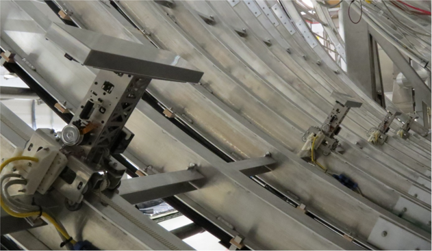
Figure 4: The four mounted mobile sensor units in their rest positions (docking stations) on the inner belts of the LFCS support structure. In the foreground the MobS unit on LFCS 3 close to the source side of the cylindrical part of the MS. Further away the MobS units on LFCS 6, 9 and 12 can be seen.

fig:RMMSConfig displays the schematic interaction of all involved RMMS subsystems and their integration with the KATRIN experiment. The upper part of the figure shows the structure of radial magnetic measuring system with the master and control module and the four installed MobSU.

Figure 5: Schematic structure of the RMMS and its integration into the KATRIN slow control system. Figure is taken from [9].

The so-called docking station (DS) is the start and end point of unit motion. It also represents the electromechanical as well as the data transfer link between the sensor unit and the master module (see [10]) which is the interface to the KATRIN slow control database. Each subsystem of the RMMS can be configured and controlled by means of the PC tool ’MagSeN-GUI’. The connection between the radial magnetic field measuring system and the data management system and the SlowControl [11] of KATRIN is realized via a modular CompactRIO Platform^® (cRIO) [12]. In addition to the communication and transmission of the data to the higher-level processing stage, the controlled charging of the batteries installed on the MobSU is also performed via an interface integrated in the cRIO. Equivalent to many other KATRIN subsystems, the measured data of the RMMS can be accessed via an ADEI interface [11]. The complete system is described in [9].

2.1 The Mobile Sensor Unit

The mobile sensor unit represents the actual sensor from the point of view of the sensor network. The prototype of the unit described in [10] has been modified and its properties improved. fig:MobSU shows the structure of the final MobSU version. The drive principle is now based on a combination of a tooth belt attached to the inner side of the LFCS support and toothed gear wheels within the MobSU drive. Due to the use of an aluminum skeleton layout of the drive chassis, the frame and the wings, a total weight of 2.9 kg is achieved with a unit height of 296 mm. The aluminum frame forms a Faraday cage and provides the necessary stiffness and electrical safety of the entire unit. The improved two-way spring-loaded chassis provides enough grip and dynamics to overcome the LFCS carrier’s structural height, lateral offsets and mechanical discontinuities along the track.

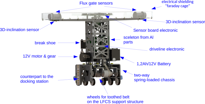
Figure 6: Mechanical structure of the mobile sensor unit with the drive, frame and wings on which the flux-gate-sensors and the inclinometers are attached. Height: 296 mm, Width: 532 mm, Weight: 2.9 kg. Distance between both flux-gate-sensors: 450 mm

Furthermore, three-dimensional inclination sensor systems based on the FXLS8471Q [14] are positioned on the wings in such a way that they are centered parallel to the flux-gate-sensors. Due to a variation in the temporal behavior of the individual components, especially due to a dependence on the battery voltage, deviations of the positioning accuracy of the unit were detected. In order to counteract these uncertainties, a control algorithm without time dependent parameters has been developed, which is described in detail in [9]. By use of an incremental encoder, the local positions of the units on their tracks are recorded with a mechanical accuracy of 48.9 $\mu$m and digital inclination accuracy of 0.37^∘ during the entire revolution around the spectrometer. tab:accurMobs shows the determined sensor system accuracies.

Sensor	Accuracy
Magnetometer	0.5% (at $\pm 1000\mu$T) $\pm$20nT
Position	48.9$\mu$m $\pm$36nm
Inclination	0.37∘ $\pm$0.0219∘

Table 1: Experimentally determined parameters for RMMS measurement accuracy after calibration process

In addition, the maximum speed is reduced in a controlled manner for the area of downward motion of the mobile unit. This procedure makes it possible to reach the target position with an accuracy better than 1 mm. fig:MobSUStopAccur shows the distribution of stopping accuracy (difference between the target and reached position) for all four MobSU based on 15 randomly selected measurement runs.

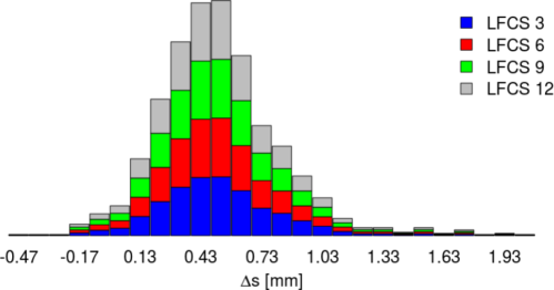
Figure 7: Distribution of the global stopping reproduction accuracy of the installed mobile units for 15 randomly selected measurement runs. Figure taken from [9].

In order to achieve the mechanical precision mentioned above, new concepts have been implemented in the motion control, as described in [9] in more detail. The necessary parameters are configured within the PC-Tool MagSeN-GUI. In particular, the desired number of magnetic field sampling positions on the entire LFCS ring must be set. The number of sampling positions (schematically shown in fig:MeasPosA) is used to calculate the required distance between the stopping positions of the mobile sensor unit which affects the total duration of one measurement cycle (see fig:MeasDur).

number of pts.	meas. duration
60	$\approx 9.5$ min
72	$\approx 10.8$ min
144	$\approx 15.8$ min

(a)

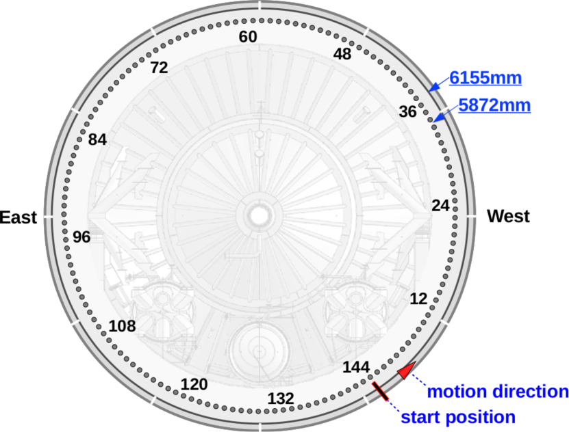
(b)

Figure 8: (a) Experimentally determined measurement duration for one measuring run depending on the configured number of positions. (b) Schematic representation of the sampling positions (dark circles) and sampling point numbers of the mobile sensor unit on the LFCS coil support structure with an average radius of 6155 mm viewed from the detector site. The average radius of the flux-gate-sensor path is 5872 mm. Starting position and motion direction are indicated.

2.2 Magnetization effect and influence of compensation systems

During the commissioning phase of the large air coil system (see [8]), the operational performance and functionality of the radial magnetic field sensor net was also inspected. For this purpose, the amperage of each individual LFCS coil was gradually adjusted and the magnetic field was recorded using the RMMS at $2*144$ measuring positions per MobSU. The 1152 points in total served as a basis for the investigation of possible magnetization effects. fig:hystdBz shows the absolute difference of the $B_{z}$-component of the magnetic field between the two flux gate magnetometers of a single sensor unit depending on the current in the associated LFCS coil, using LFCS 6 as an example. The black dashed line indicates the position of the slice for the hysteresis view in fig:hystdBzb. It should be noted that all values used are in inclination corrected local MobSU coordinates.

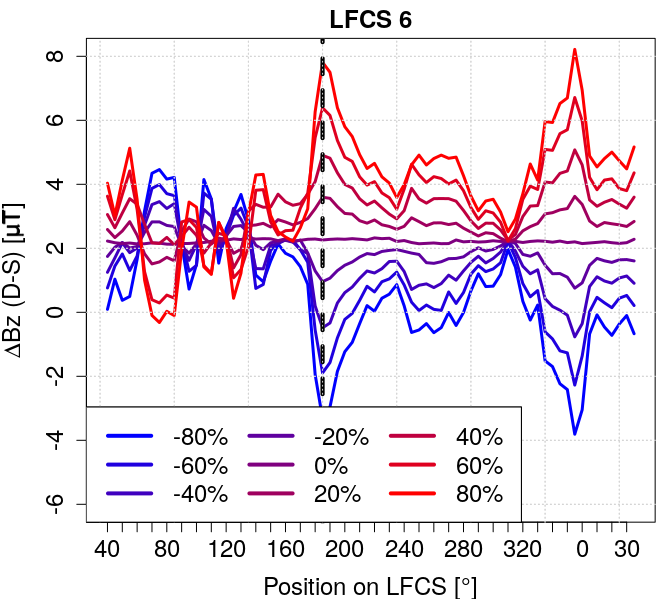
(a)

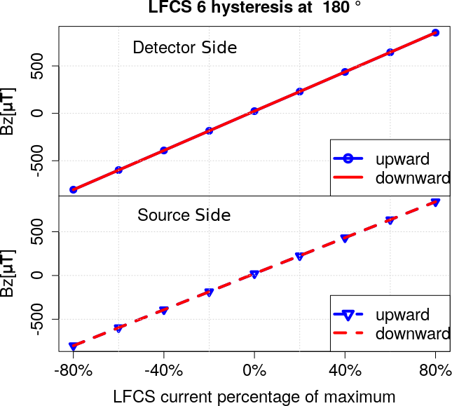
(b)

Figure 9: a) Absolute difference for $B_{z}$-component of the magnetic field between the two MobSU magnetometers for different percentages of LFCS current settings in steps of $20\%$ of the full current. Full currents used (100%): 100 A for LFCS 1,2,12,13, 115 A for LFCS 3…11 and 70 A for LFCS 14. The MobSU position is shown in degree of rotation along the axis of the abscissas. Figure taken from [9]. b) Hysteresis view at position of 180^∘ on the LFCS 6.

2.3 Coordinate system transformation and field determination in the analyzing plane

Due to the slight deformations and a possible misalignment of the LFCS (see [8]) the transformation of the locally obtained magnetic field values into a more global KATRIN coordinate system [16] is problematic. However, on the basis of the LFCS deformation measurement [17] (data listing the radii of the LFCS at 36 angles along the circumference) a first attempt has been made. The deviation of the LFCS radii from the ideal $R_{i}=6.155$ m at the sampling positions can be approximated iteratively by a spline interpolation taking into account the manually determined start positions and angles at the docking station. Based on this, the distance traveled by the sensor unit can be taken as the arc length $S$ of the LFCS circle to determine the global position $t_{x,y,z}$ of the unit under the condition $S_{Model}\equiv S_{MobSU}$.

$$S_{Model}=A_{corr}\cdot\int_{\alpha_{Dock}}^{\alpha_{th}}\sqrt{\left(R^{2}+\left({{\partial R}\over{\partial\alpha}}\right)^{2}\right)_{\alpha=u}}du$$ (1)

$$t_{x}=R\cdot cos(\alpha_{th})\qquad t_{y}=R\cdot sin(\alpha_{th})\qquad t_{z}=t_{z}$$ (2)

$A_{corr}=\frac{s_{Dock}}{s_{Model}}$ represents a standardization constant at $\alpha_{th}=\alpha_{Dock}$ condition where $\alpha_{th}$ indicates the numerically determined theoretical rotation angle of MobSU. The experimentally determined positional data for the position in the z-direction $t_{z}$, the LFCS total circumference $S_{Dock}$ and the start or end angle $\alpha_{Dock}$ of the MS revolution are summarized in tab:PosDataForSpline.

	LFCS 3	LFCS 6	LFCS 9	LFCS 12
$t_{z}$ [m] ([mm])	-4.040 (5)	-1.338 (5)	1.354 (5)	4.058 (5)
$s_{Dock}$ [m] ([mm])	38.715 (3.96)	38.705 (3.89)	38.745 (3.11)	38.678 (3.23)
$\alpha_{Dock}$ [∘]	36.86 (0.175)	36.04 (0.216)	37.03 (0.307)	37.07 (0.349)

Table 2: Data of the LFCS support beams : $t_{z}$ the position in z direction relative to the MS center, $S_{Dock}$ the total arc of sensor path for 1 revolution and $\alpha_{Dock}$ the start value for the inclination. The numbers in brackets represent the absolute deviation determined by using several unit runs.

With the sensor element orientation shown in fig:mCoords, the known theoretical rotation angle $\alpha_{th}$ and the measured inclination angles $\vec{g}_{DS}$ and $\vec{g}_{SS}$ of both MobSU magnetometer, the inclination corrected rotation matrix $M_{rot}$ can be created.

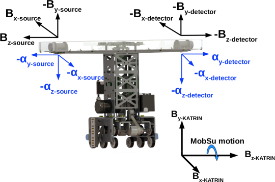
Figure 10: Orientation of the sensor components of the mobile sensor unit. Movement sequence of the unit around the spectrometer corresponds to the rotation around the longitudinal center axis of the MS (the z-axis of the global KATRIN coordinate system). Figure adopted from [9].

$$M_{rot}=N_{MobSU}\cdot N_{Trans}\cdot K$$ (3)

Where $N_{MobSU}$ represents an ideal rotation matrix based on $\alpha_{th}$, $N_{Trans}$ specifies the MobSU construction-related translation matrix and $K$ indicates the inclination correction matrix. A more detailed description is given in [9]. The coordinate transformation has a considerable influence on the total error of the magnetic field measurement, $\overrightarrow{\Delta B}$ which is calculated according to eq:BError and is shown in fig:BFehler. It should be noted that all of the magnetic field errors on the Detector Side (DS) and the Source Side (SS) correlate in different ways. This can be explained by inaccuracies and deviations of the mathematical model of coordinate transformation presented here. As the overall error is relatively small, this aspect can be neglected. To achieve better results, an improvement of the model data from [17] by at least a factor of 10 is necessary.

$$\overrightarrow{\Delta B}=M_{rot_{DS/SS}}\cdot{{\overrightarrow{\sigma_{B}}_{DS/SS}}\over{\sqrt{32}}}+\overrightarrow{\Delta g}_{max}\cdot|B_{DS/SS}|$$ (4)

$M_{rot}$ specifies the mentioned corrected rotation matrix for the individual magnetometer, $\overrightarrow{\sigma_{B}}$ represents the corresponding uncertainty of the magnetic field measurement and $\overrightarrow{\Delta g}_{max}$ indicates the maximum error of the MobSU internal inclination system.

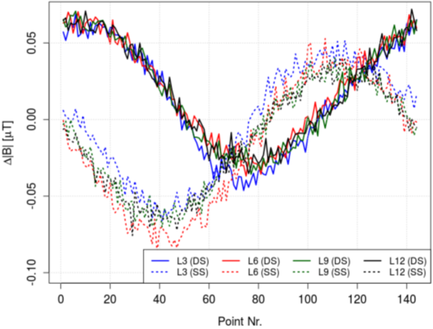
Figure 11: Total error of the magnetic field $\Delta|B|$ after transformation into the KATRIN coordinate system. Figure based on [9].

The availability of the measured values in KATRIN coordinates allows a direct comparison with simulated values. On the other hand one can use interpolation methods to derive magnetic field values inside the MS volume. The magnetic field in the analyzing plane as a result of a bi-linear interpolation on an irregular grid performed in [9] is shown in fig:MidSlice. This method covers 86% of the total analyzing plane area.

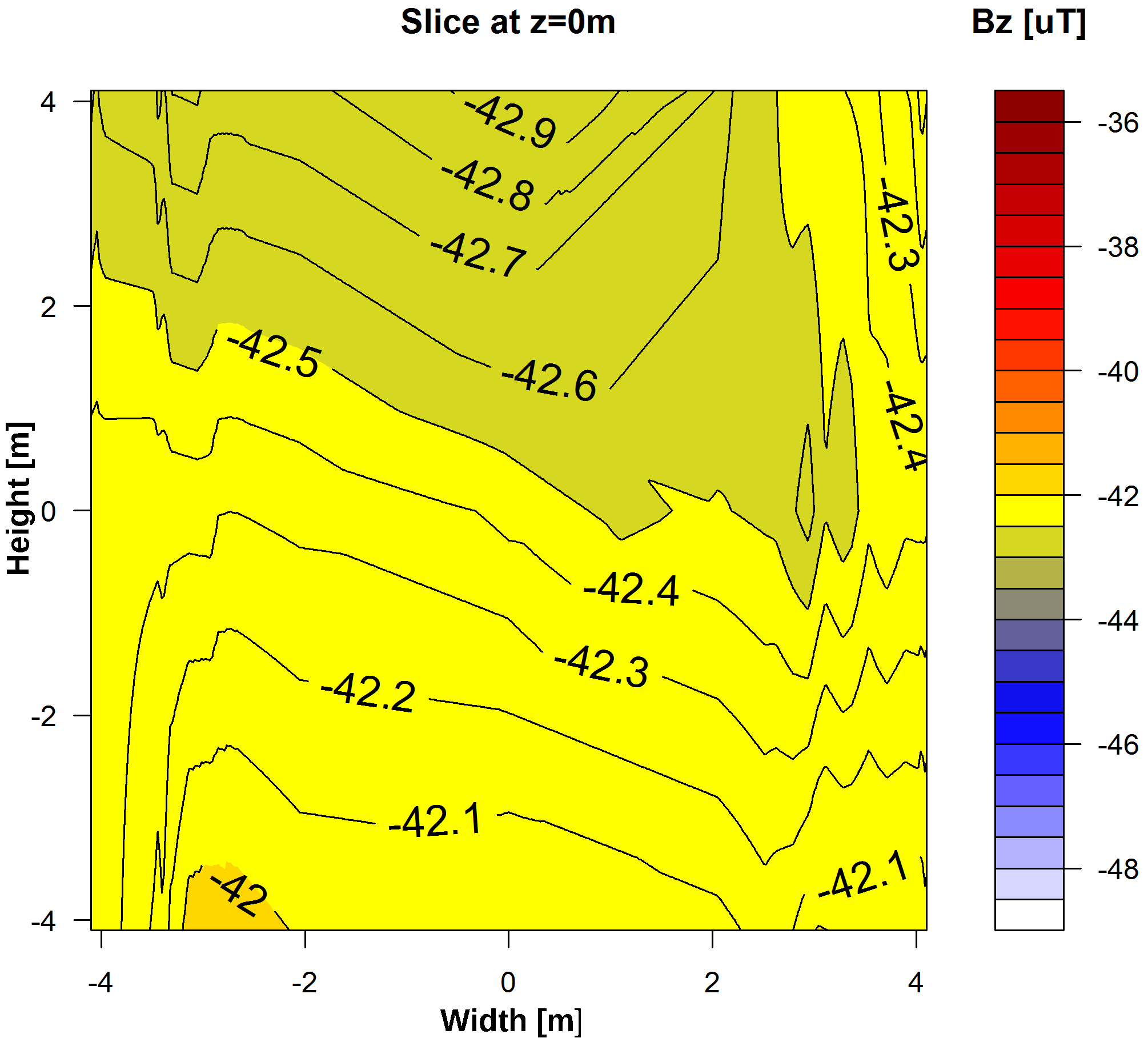
(a)

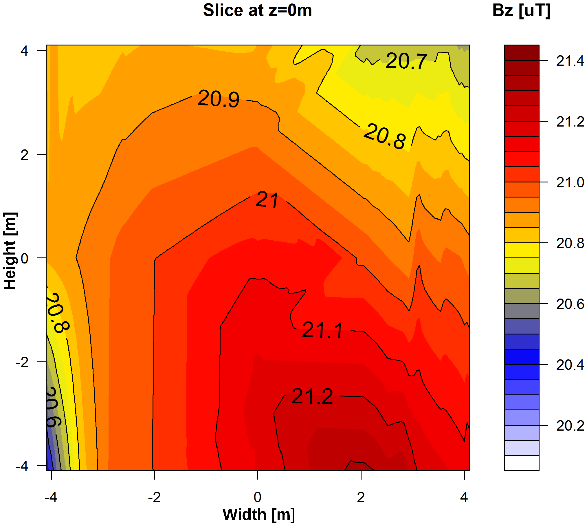
(b)

Figure 12: Interpolation results of $B_{z}$ in the analysis plane (center of the MS) for (a) detector magnet at 2.5 T, pinch magnet at 4.2 T and PS at 3.1 T, all other magnets off (b) all magnets off, only earth magnetic field.

3 The vertical magnetic field measuring system

Magnetic field investigations in the immediate environment of the MS revealed both remanent and induced magnetization effects of the hall walls which have a direct influence on the magnetic field in the analysis plane (see [19]). For this reason, a vertical magnetic measuring system (VMMS) covering vertical planes parallel to hall walls has been developed. Mechanically, the VMMS is inspired by the technology of the MobSU and is based on a movable construction of linear rails which are attached to the hall pillars.

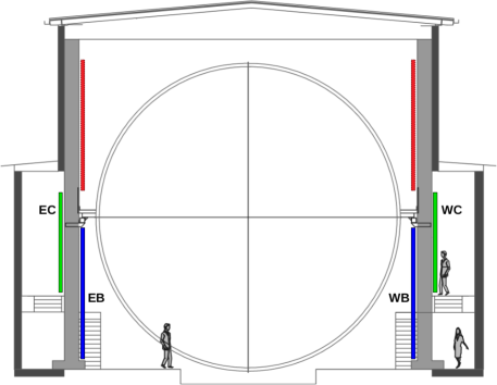
Figure 13: Schematic representation of the VMMS position within the KATRIN MS hall. Individual layers are color-coded. View from the north. Individual systems are marked with EC (east center), EB (east bottom), WC (west center) and WB (west bottom).

In terms of measuring accuracy and positioning precision, all requirements are met equivalent to the system of the mobile sensor units. The aim is to completely cover the wall surface in the area of the cylindrical MS vessel at three height levels and to measure the magnetic field with a mesh width of 20 cm x 20 cm. At the current stage four VMMS at two height levels are installed and commissioned. fig:VMMSHall shows the position of the individual systems. The construction of the upper system (in red) is currently in the concept phase and will be finished in the near future.
fig:VMMSmech shows the schematic structure of such a VMMS system in a CAD view. The two movable components (horizontal and vertical), the movement limited hinge to prevent inadmissibly strong pendulum movement during the movement, as well as the drive chains connecting the subsystems and the cable duct can be seen.

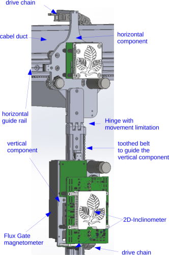
Figure 14: Schematic structure of the VMMS system in a CAD view.

The movement sequence is as follows: the vertical component starts in the lowest position and moves upwards to the next sampling position at a distance of 20 cm. After the measurement has been carried out at this point, it moves to the next sampling position. As soon as the end of the vertical linear rail has been reached, the horizontal component is moved to the next position and the vertical system returns back to the initial point. After reaching the overall target position, the above procedure is repeated. In this way, a grid of magnetic field measuring points is built up until the end of the horizontal linear rail is reached. tab:VKenngr shows a listing of the most important parameters of the VMMS with regard to track length, total measuring time and total number of measuring positions. Using the already mentioned method of bilinear interpolation on irregular grids, a more detailed investigation of the influence of magnetization effects on hall walls can be carried out. Using the EC component of VMMS as an example, the interpolation results of the magnetic field magnitude $|\vec{B}|$ are shown in the fig:MagVInterpol_Earth.

	EB	EC	WB	WC
vertical track length [m]	4.40	2.60	4.60	2.60
horizontal track length [m]	20.20	21.00	20.80	21.00
measuring positions	2346	1484	2520	1484
measuring time [h]	5.68	3.85	6.16	3.85

Table 3: Significant parameters in relation to the track length, number of measuring positions and total measuring time of individual VMMS systems.

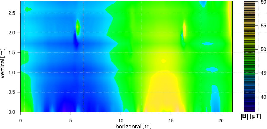
Figure 15: Interpolation result of the earth magnetic field measurement $|\vec{B}|$ in $\mu$T using 1484 sampling positions of the EC VMMS.

4 Summary and Outlook

In order to inspect the magnetic field inside the KATRIN main spectrometer during normal operation, two high-resolution magnetic sensor systems have been developed and combined to form a fine-meshed magnetic sensor network. Depending on the mesh size, several thousand magnetic field samples can be taken close to the surface of the MS (RMMS) and on vertical planes left and right of the main spectrometer (VMMS). The electromechanical features of the mobile sensor units have been investigated and the serviceability of the systems has been demonstrated. It has also been shown that the magnetic field at the analyzing plane $B_{A}$, formed by the MS spectrometer magnets inside the main spectrometer, can be derived from the RMMS magnetic field samples by interpolation. However, with more refined interpolation strategies and methods like the Laplace method [18] the stability of the result should be investigated. Moreover, as the error connected with interpolation numerics generally varies with $1/N$, with $N$ being the number of sampling points, the installation of 2 more units on LFCS 7 and LFCS 8 adjacent to the analyzing plane is advisable.
Furthermore, model based simulations of the magnetic field can be checked and improved by magnetic field samples at the MS site. Especially the magnetic dipoles method [20] needs several thousand B-field samples from RMMS and VMMS. Using this method the magnetization of model dipoles (several hundreds) can be determined and represented in simulations.

The authors wish to express gratitude to the group for Experimental Techniques of the Institute for Nuclear Physics (IKP) at KIT and for highly efficient and competent support. Furthermore, we wish to thank Prof. Dr. E. W. Otten, Mainz University for helpful discussions and support. In addition, we like to thank the University of Applied Sciences, Fulda and the Fachbereich Elektrotechnik und Informationstechnik for their support during the entire process.

This work has been funded by the German Ministry for Education and Research under the Project codes 05A14REA, 05A11REA, 05A08RE1

References

- [1] KATRIN Collaboration, KATRIN Design Report, 2004, FZKA scientific report 7090, \hrefhttp://bibliothek.fzk.de/zb/berichte/FZKA7090.pdf http://bibliothek.fzk.de/zb/berichte/FZKA7090.pdf.
- [2] V.M. Lobashev, P.E. Spivac, A method for measuring the anti-electron-neutrino rest mass, Nucl. Instrum. Meth. A240 (1985), 305.
- [3] H. Backe, J. Bonn, Th. Edling, H. Fischer, A. Hermanni, P. Leiderer, Th. Loeken, R.B. Moore, A. Osipowicz, E. W. Otten, A Picard A solenoid retarding spectrometer and an atomic tritium source for use in a neutrino mass experiment, Proc.of the VIIth Moriond Workshop on “New and Exotic Phenomena”, Les Arcs, France,1987 (O. Fackler, J.Tran Thanh Van, eds.) Editions Frontiers, Gif-sur-Yvette, France 1987, p.297.
- [4] A.Picard et.al, A solenoid retarding spectrometer with high resolution and transmission for keV electrons, Nucl. Instrum. Meth. B 63 (1992) 345.
- [5] W. Gill et.al, The KATRIN Superconducting Magnets: Overview and First Performance Results, arXiv:1806.08312, 2018
- [6] B. Zipfel, PartOpt Precision field calculation and Particle Optics design, 2002, http://www.partopt.net.
- [7] A. Osipowicz and F. Glück, Air coil design at the MS,14. KATRIN Collaboration Meeting, 2008,http://fuzzy.fzk.de/bscw/bscw.cgi/d443733/95-TRP-4440-D1-FGlueck-AOsipovicz.ppt.
-
[8]
M. Erhard et al.,