A diffuse interface model for the analysis of propagating bulges in cylindrical balloons

Abstract

With the aim to characterize the formation and propagation of bulges in cylindrical rubber balloons, we carry out an expansion of the non-linear axisymmetric membrane model assuming slow axial variations. We obtain a diffuse interface model similar to that introduced by van der Waals in the context of liquid-vapor phase transitions. This provides a quantitative basis to the well-known analogy between propagating bulges and phase transitions. The diffuse interface model is amenable to numerical as well as analytical solutions, including linear and non-linear bifurcation analyses. Comparisons to the original membrane model reveal that the diffuse interface model captures the bulging phenomenon very accurately, even for well-localized phase boundaries.

1 Introduction

1.1 Problem and background

Bulges in cylindrical rubber balloons are a classical example of localization in solid mechanics. When a balloon is inflated, an initial regime of uniform inflation is followed by the formation of a bulge: the bulge appears initially as a long-wavelength buckling mode that localizes rapidly and then grows locally, until it propagates and eventually invades the entire balloon [1]. As in other localization phenomena, the formation of a bulge reflects the non-convexity of the strain energy when restricted to homogeneous deformations: the onset of bulging occurs quickly after the maximum in the volume-pressure loading curve, and the propagation pressure can be predicted by Maxwell’s equal-area rule [2].

Several other localization phenomena have been studied in solid mechanics, such as stress-induced phase transformations [3, 4, 5], the necking of bars [6, 7, 8], kink bands in compressed fiber composites [9, 10], as well as localized structures in thin elastic shells [11] and tape springs [12, 13].

These localization phenomena have been investigated based on two types of models, as discussed in [14] for example. On the one hand, non-regularized models, also known as sharp interface models, make use of a classical strain energy functional depending solely on the strain: the onset of localization is associated with the loss of ellipticity of the equations of equilibrium at a critical value of the load [15]. Such models can typically predict the critical load, the formation of different phases and the orientation of the phase boundaries, but cannot predict their subsequent evolution, nor their number or distribution in space; they cannot resolve the displacement inside the localized region either. On the other hand, regularized models, also known as diffuse interface models, make use of a stored elastic energy functional depending on both the strain and the strain gradient: such models remedy the limitations of the non-regularized models, and in particular remain well posed beyond the onset of localization [16].

Regularized models are often introduced heuristically, but can in some cases be justified mathematically. Such a justification has been done in the case of periodic elastic solids, such as elastic crystals [17, 18], trusses made of elastic bars or beams [19], or elastic solids with a periodic micro-structure [14, 20]. In these works on periodic solids, the ratio $R/L\ll 1$ of microscopic cell size $R$ to the macroscopic dimension $L$ of the structure is used as an expansion parameter, and the homogenized properties of the periodic medium are derived through a systematic expansion in terms of the macroscopic strain and of its successive gradients.

The goal of this paper is to derive a one-dimensional, regularized model applicable to the analysis of axisymmetric bulges in cylindrical rubber balloons. It is part of a general effort to characterize localization phenomena occurring in slender structures, which have been much less studied than in periodic solids. In slender structures, regularized models can be derived by an asymptotic expansion as well, using now the aspect ratio $R/L\ll 1$ as the expansion parameter where $R$ is the typical transverse dimension of the structure and $L$ its length. This approach has been carried out for the analysis of necking, and diffuse interface models have been derived asymptotically, first for a two-dimensional hyperelastic strip by Mielke [21] and later for a general prismatic solid in three dimensions by Audoly & Hutchinson [22]. These authors proposed an expansion method upon which we build ours (and which we improve).

Our asymptotic expansion starts from the axisymmetric membrane model, which has been used extensively to analyze bulges in cylindrical balloons [23, 1]. Its outcome is a one-dimensional diffuse interface model, exactly similar to that introduced heuristically by van der Waals [24] to analyze the liquid-vapor phase transitions at a mesoscopic level. The analogy between bulges in balloons and phase transitions has been known for a long time: Chater & Hutchinson [2] have adapted Maxwell’s rule for the the coexistence of two phases to derive the pressure at which a bulge can propagate in a balloon, while Müller & Strehlow [25] have proposed a pedagogical introduction to the theory of phase transitions based on the mechanics of rubber balloons. Here, we push the analogy further, and show that the diffuse interface model can provide a quantitative description of bulges in balloons, not only accounting for the propagation pressure, but also for the domain boundary between the bulged and unbulged phases, as well as for its formation via a bifurcation—borrowing from the theory of phase transitions, we will refer to this boundary as a ‘diffuse interface’. The diffuse interface model is classical, tractable, and amenable to analytical bifurcation and post-bifurcation analysis, as we demonstrate. It is also simpler than the axisymmetric membrane model on which it is based.

There is a vast body of work on the bulging of cylindrical balloons, all of which have used the theory of axisymmetric membranes as a starting point. The stability and bifurcations from homogeneous solutions have been analyzed in [26, 27, 28]. Non-linear solutions comprising bulges have been derived in [29]. The analysis of stability has been later extended to arbitrary incompressible hyperelastic materials, to various closure conditions at the ends of the tube, as well as to various type of loading controls based on either the internal pressure, the mass or the volume of the enclosed gas [30]. In a recent series of four papers, Fu et al. [31, 32, 33, 34] revisit the bifurcation problem, complement it with the weakly non-linear post-bifurcation analysis in the case of an infinite tube, and address imperfection sensitivity. Besides these theoretical studies, there has been a number of experimental and numerical papers on balloons. A compelling agreement between experiments and numerical simulations of the non-linear membrane model has been obtained by Kyriakides & Chang [23, 1], who provide detailed experimental and numerical results on the initiation, growth and propagation of bulges, highlighting the analogy with phase transitions. Given that the agreement between experiments and the non-linear membrane theory has already been covered thoroughly in this work, our focus here will be on comparing the diffuse interface model to the non-linear membrane model, using exactly the same material model as in Kyriakides’ simulations and experiments.

1.2 Outline of the main results

Our work focusses on solutions to the non-linear axisymmetric membrane model that vary slowly in the axial direction, as happens typically at the onset of localization. A systematic expansion of the membrane energy is obtained in terms of the aspect-ratio parameter $\varepsilon=R/L\ll 1$, where $R$ is the initial radius of the balloon and $L$ its initial length. The result reads

$$\mathcal{E}[p,\mu]=\int_{0}^{L}\left[G_{0}(p,\mu(Z))+\frac{1}{2}B_{0}(p,\mu(Z))\mu^{\prime 2}(Z)\right]\mathrm{d}Z$$ (1)

where $p$ denotes the (scaled) internal pressure, a control parameter in the experiments, $Z$ is the axial coordinate and $\mu(Z)$ is a strain measure, see figure 1. Specifically, $\mu$ is the orthoradial stretch, defined as the ratio $\mu(Z)=\frac{r(Z)}{R}$ of the current radius $r$ to the initial radius.

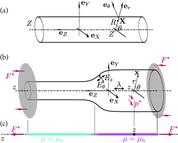
Figure 1: Inflation of a cylindrical membrane: (a) reference configuration, (b) sketch of an equilibrium configuration when the membrane is subject to an axial force $F$ and an internal pressure $p$. (c) Equivalent diffuse interface model derived in this paper: a bar having an order parameter $\mu(Z)$ undergoes a phase transformation.

The potential $G_{0}$ appearing in the first term is a non-convex function of the stretch $\mu$, much like in Ericksen’s bar [3]: the non-regularized model for the balloon would correspond to the energy functional $\int_{0}^{L}G_{0}(p,\mu(Z))\,\mathrm{d}Z$. Values of $p$ such that several minima of $G_{0}$ exist correspond to pressures for which different phases (associated with different values of the stretch $\mu$) are in competition. The second term $\frac{1}{2}\,B_{0}\,\mu^{\prime 2}$ in the integrand is a correction of order $\varepsilon^{2}$, that accounts for the energetic cost of inhomogeneity; in the theory of phase transitions, this is the term that would account for surface tension at an interface.

We provide simple and explicit formulas for both the potential $G_{0}$ characterizing homogeneous solutions, see §3, equations (9), (11) (13) and (14) in particular, and for the modulus $B_{0}$ of the regularizing term, see §4 and equation (20b).

The diffuse interface model is obtained by a systematic, formal expansion. It is asymptotically exact and does not rely on any unjustified kinematic assumptions: equation (1) approximates the energy of the original membrane model with an error of order $\varepsilon^{4}$ that is negligible compared to the smallest term retained, namely the gradient term of order $\varepsilon^{2}$. By contrast, regularized models for slender structures have been proposed in earlier work starting from kinematic hypotheses, which appeared to be incorrect: see the treatment of necking in an elastic cylinder in [35] as well as the critical discussion in [22].

Our derivation is based on a finite-strain membrane model. The non-linear features of the elastic constitutive law at finite strain are ultimately reflected in the diffuse interface model through the non-linear potential $G_{0}(p,\mu)$ and through the dependence of the second gradient coefficient $B_{0}(p,\mu)$ on the current strain $\mu$. By contrast, an assumption of small strain has been used in previous work [36, 37] on the justification of a diffuse interface model to analyze phase transformations in an elastic cylinder: this assumption is questionable since the presence of coexisting phases involves finite variations of strain across the interface.

The outline of the paper is as follows. In §2, we introduce the non-linear membrane model. In §3 we analyze its homogeneous solutions, and derive an expression for the potential $G_{0}$. Section 4 is the core of the paper, and establishes the diffuse interface model (1) by an asymptotic method. Section 5 derives solutions to the diffuse interface model using various methods, and compares them with the predictions of the original membrane model.

2 Non-linear membrane model

We consider a cylindrical membrane with uniform initial thickness $H$ and radius $R$. We use the cylindrical coordinates $(Z,\theta)$ in reference configuration as Lagrangian variables. When subject to external load, the cylinder deforms into an axisymmetric membrane, see figure 1a. The cylindrical coordinates of a material point in actual configuration are written as $(r(Z),\theta)$, corresponding to a position $\mathbf{x}(Z,\theta)=z(Z)\,\mathbf{e}_{z}+r(Z)\,\mathbf{e}_{r}(\theta)$, where $(\mathbf{e}_{r}(\theta),\mathbf{e}_{\theta}(\theta),\mathbf{e}_{z})$ is the local cylindrical basis.

In the axisymmetric membrane theory, the deformation gradient is a $3\times 2$ matrix which writes

$$\mathbf{F}=\mu\,\mathbf{e_{\theta}}\otimes\mathbf{e}_{\theta}+(R\,\mu^{\prime}\,\mathbf{e}_{r}+\lambda\,\mathbf{e}_{z})\otimes\mathbf{e}_{z}$$

where we have defined an apparent axial stretch $\lambda$ and the circumferential stretch $\mu$ as

$$\lambda(Z) =\frac{\mathrm{d}z}{\mathrm{d}Z}(Z),$$ (2a)

$$\mu(Z) =\frac{r(Z)}{R}.$$ (2b)

The Green-Lagrange strain tensor $\mathbf{E}=\frac{1}{2}(\mathbf{F}^{T}\cdot\mathbf{F}-\mathbf{1})$ is a $2\times 2$ diagonal matrix in the basis $(\mathbf{e}_{\theta},\mathbf{e}_{z})$ tangent to the undeformed mid-surface: it will be represented compactly as a vector, whose entries are the diagonal components $E_{\theta}$ and $E_{z}$ of the matrix,

$$\mathbf{E}(\lambda,\mu,\mu^{\prime})=\left(\begin{array}[]{c}E_{\theta}\\ E_{z}\end{array}\right)=\frac{1}{2}\begin{pmatrix}\mu^{2}-1\\ \lambda^{2}+(R\mu^{\prime})^{2}-1\end{pmatrix},$$ (3)

where $\mu^{\prime}=\frac{\mathrm{d}\mu}{\mathrm{d}Z}$ is a stretch gradient, namely the axial gradient of circumferential stretch.

A material model is now specified through a strain energy per unit volume $w^{*}(E_{\theta},E_{z})$. In previous work on axisymmetric membranes [23, 1, 31], the 2d material model proposed by Ogden [38] for incompressible rubber has been used:

$$w^{*}(E_{\theta},E_{z})=\sum_{i=1}^{3}\frac{S_{i}}{\alpha_{i}}\left(\ell_{\theta}^{\alpha_{i}}+\ell_{z}^{\alpha_{i}}+\left(\frac{1}{\ell_{\theta}\ell_{z}}\right)^{\alpha_{i}}\right),\quad\textrm{with }\begin{cases}\ell_{\theta}=\sqrt{2E_{\theta}+1}&\textrm{(circumfer.\ stretch)}\textrm{,}\\ \ell_{z}=\sqrt{2E_{z}+1}&\textrm{(axial stretch)}\textrm{.}\end{cases}$$ (4)

We use this model as well for our numerical examples, with the same set of material parameters $\alpha_{i}$’s and $S_{i}$’s as used in previous work, namely $S_{1}=617$ kPa, $S_{2}=1.86$kPa, $S_{3}=-9.79$kPa, $\alpha_{1}=1.3$, $\alpha_{2}=5.08$ and $\alpha_{3}=-2$. All our results can be easily adapted to a different constitutive law. For this constitutive law, the initial shear modulus $S_{\mathrm{ini}}$ can be obtained as $S_{\mathrm{ini}}=\sum_{i=1}^{3}\alpha_{i}\,S_{i}$.

The domain $0\leq Z\leq L$ represents one half of a balloon comprising a single bulge center at $Z=0$, with symmetry conditions $\mu^{\prime}=\lambda^{\prime}=0$ enforced at $Z=0$. At the other endpoint $Z=L$, we consider the ideal boundary conditions sketched in figure 1b, whereby the terminal section of the balloon is resting and freely sliding on a planar ‘plug’. These conditions would be difficult to achieve in experiments but they offer the advantage of being compatible with a uniform expansion of the membrane, which simplifies the analysis. By contrast, actual cylindrical balloons are typically closed up on their ends and cannot be inflated in a homogeneous manner due to end effects; these end effects could reproduced by employing different boundary conditions, but we prefer to ignore them. Note that Kyriakides & Chang[23, 1] use a rigid plug condition on one end, $\mu(L)=1$, which is not realistic either. Our boundary conditions, sketched in figure 1 and provided in explicit form in §55.1, are natural: the applicable equilibrium condition will emerge automatically from the condition that the energy is stationary.

As in the experiments of Kyriakides & Chang [1], the membrane is subject to an interior pressure $p^{\ast}$ and to a stretching force $F^{\ast}$ applied along the axis, see figure 1. The total potential energy reads

$$\mathcal{E}_{\mathrm{memb}}^{\ast}=\int_{0}^{L}\Big{(}w^{*}(\mathbf{E})\,2\,\pi\,R\,H\,\mathrm{d}Z-\pi\,(R\,\mu)^{2}\,(\lambda\,\mathrm{d}Z)\,p^{\ast}-(\lambda\,\mathrm{d}Z)\,F^{*}\Big{)}$$

where $2\,\pi\,R\,H\,\mathrm{d}Z$ is the initial volume element, $\pi\,(R\,\mu)^{2}\,(\lambda\,\mathrm{d}Z)=\pi\,r^{2}\,\mathrm{d}z$ is the current enclosed volume element, and $\lambda\,\mathrm{d}Z=\mathrm{d}z$ is the current axial length element.

We introduce a rescaled energy, denoted without an asterisk as $\mathcal{E}_{\mathrm{memb}}=\frac{\mathcal{E}_{\mathrm{memb}}^{\ast}}{(2\pi\,R\,H)\,S_{\mathrm{ini}}}$:

$$\mathcal{E}_{\mathrm{memb}}[p,\lambda,\mu]=\int_{0}^{L}\left(w(\mathbf{E}(\lambda,\mu,\mu^{\prime}))-p\frac{e}{2}\,\lambda\,\mu^{2}-F\lambda\right)\mathrm{d}Z\textrm{.}$$ (5)

The strain energy, the force and pressure have been rescaled as well, as $w=\frac{w^{*}}{S_{\mathrm{ini}}}$, $F=\frac{F^{\ast}}{2\pi RHS_{\mathrm{ini}}}$ and $p=\frac{p^{\ast}}{S_{\mathrm{ini}}}$, respectively, and $e=\frac{R}{H}$ is an initial aspect ratio. In our numerical examples, we use the same value $e=\frac{55}{16}$ as in [1]: even though this balloon is relatively thick prior to deformation, the non-linear membrane model has been checked to match the experimental results accurately in [1]. We also use the same value of the load

$$F=1.149$$ (6)

as in these experiments. The parameter $F$ will never be changed, and we do not keep track of how the various quantities depend on $F$; the argument $F$ will systematically be omitted in functions, as we did already in the left hand side of (5).

The functions $\lambda(Z)$ and $\mu(Z)$ that make the energy (5) stationary yield the axisymmetric equilibra of the balloon. These solutions are obtained by a numerical method described in section 55.1, and are plotted as the black curves in figure 3, where they are used as a reference.

3 Analysis of homogeneous solutions

Our general goal is to justify the diffuse interface model when $\lambda(Z)$ and $\mu(Z)$ vary slowly as a function of $Z$. In this section, we start by considering the case where $\lambda$ and $\mu$ do not depend on $Z$,

$$\frac{\mathrm{d}\lambda}{\mathrm{d}Z}=0,\qquad\frac{\mathrm{d}\mu}{\mathrm{d}Z}=0\textrm{.}$$ (7)

This corresponds to homogeneous solutions, i.e. to solutions with uniform inflation. These homogeneous solutions are well known, and are re-derived here for the sake of completeness. A catalog of such homogeneous solutions will be obtained, which plays a key role in the subsequent derivation of the diffuse interface model.

3.1 Kinematics of homogeneous solutions

For homogeneous solutions, the gradient term $\mu^{\prime}$ in (3) vanishes and the membrane strain reads

$$\mathbf{E}_{0}(\lambda,\mu)=\begin{pmatrix}E_{0}^{\theta}\\ E_{0}^{z}\end{pmatrix}=\frac{1}{2}\left(\begin{array}[]{c}\mu^{2}-1\\ \lambda^{2}-1\end{array}\right).$$ (8)

All the quantities pertaining to homogeneous solutions are denoted using a subscript ‘$0$’. In the homogeneous case, the strain energy becomes

$$w_{0}(\lambda,\mu)=\frac{1}{S_{\mathrm{ini}}}\sum_{i=1}^{3}\frac{S_{i}}{\alpha_{i}}\left(\lambda^{\alpha_{i}}+\mu^{\alpha_{i}}+\left(\frac{1}{\lambda\,\mu}\right)^{\alpha_{i}}\right)\textrm{.}$$ (9)

Of particular importance will be the second Piola-Kirchhoff membrane stress $\boldsymbol{\Sigma}_{0}$, defined as the gradient of the strain energy with respect to the strain:

$$\boldsymbol{\Sigma}_{0}(\lambda,\mu)=\begin{pmatrix}\Sigma_{0}^{\theta}\\ \Sigma_{0}^{z}\end{pmatrix}=\begin{pmatrix}\frac{\partial w}{\partial E_{\theta}}\\ \frac{\partial w}{\partial E_{z}}\end{pmatrix}_{\mathbf{E}=\mathbf{E}_{0}}=\begin{pmatrix}\frac{1}{\mu}\frac{\partial w_{0}}{\partial\mu}(\lambda,\mu)\\ \frac{1}{\lambda}\frac{\partial w_{0}}{\partial\lambda}(\lambda,\mu)\end{pmatrix}\textrm{.}$$ (10)

3.2 Equilibrium of homogeneous solutions

In view of (5), the total potential energy of a homogeneous solution per unit reference length is

$$g_{0}(p,\lambda,\mu)=w_{0}(\lambda,\mu)-p\frac{e}{2}\,\lambda\,\mu^{2}-F\lambda.$$ (11)

Given the load parameters $p$ (and $F$) the equilibrium values of $\lambda$ and $\mu$ are found by the condition of equilibrium in the axial and transverse directions,

$$\frac{\partial g_{0}}{\partial\lambda}(p,\lambda,\mu) = 0,$$ (12a)

$$\frac{\partial g_{0}}{\partial\mu}(p,\lambda,\mu) = 0.$$ (12b)

We leave the load $p$ left unspecified for the moment, and we view the axial equilibrium (12a) as an implicit equation for $\lambda=\lambda_{0}(p,\mu)$ in terms of $p$ and $\mu$: by definition, $\lambda_{0}(p,\mu)$ is the solution to the implicit equation

$$\frac{\partial g_{0}}{\partial\lambda}(p,\lambda_{0}(p,\mu),\mu)=0.$$ (13)

From now on, we will systematically eliminate $\lambda=\lambda_{0}(p,\mu)$ in favor of the second unknown $\mu$. Starting with the potential $g_{0}$, we define a reduced potential $G_{0}$ as

$$G_{0}(p,\mu)=g_{0}(p,\lambda_{0}(p,\mu),\mu)\textrm{,}$$ (14)

as well as the stress $n_{0}$ dual to $\mu$,

$$n_{0}(p,\mu)=-\frac{\partial G_{0}}{\partial\mu}(p,\mu)\textrm{.}$$ (15a)

This $$n_{0}(p,\mu)$$ can be interpreted as an imbalance of hoop stress; it vanishes at equilibrium,

$$n_{0}(p,\mu)=0.$$ (15b)

Indeed, we have $n_{0}=-\frac{\partial G_{0}}{\partial\mu}=-\frac{\mathrm{d}g_{0}(p,\lambda_{0}(p,\mu),\mu)}{\mathrm{d}\mu}=-\frac{\partial g_{0}}{\partial\mu}-\frac{\partial\lambda_{0}}{\partial\mu}\frac{\partial g_{0}}{\partial\lambda}$, where the both terms are zero by the equilibrium conditions (12b–13).

To summarize, we view $\lambda$ as an internal variable slaved to the ‘macroscopic’ variable $\mu$ (the roles of $\lambda$ and $\mu$ could be exchanged but the other way around would be more complicated as the mapping from $\lambda$ to $\mu$ is not single-valued). A catalog of homogeneous solutions can be obtained by (i) solving the axial equilibrium (12a) for $\lambda=\lambda_{0}(p,\mu)$, (ii) defining a reduced potential energy $G_{0}(p,\mu)$ by (14), and (iii) solving the equilibrium condition $n_{0}(p,\mu)=0$ in the $(p,\mu)$ plane.

This program has been carried out and the results are shown in figure 2.

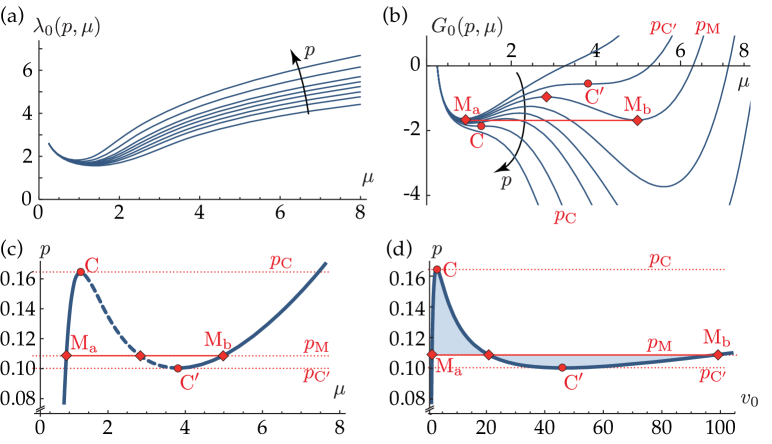
Figure 2: Analysis of the homogeneous solutions, with $F=1.149$. (a) For any value of the pressure $p$, the axial equilibrium (13) yields an implicit curve in the $(\mu,\lambda)$ plane that defines the stretch $\lambda_{0}(p,\mu)$ in terms of $\mu$; the different curves correspond to $p=0.0885,0.1002,0.1087,0.1187,0.1285,0.140,0.1646,0.200$. (b) Reduced potential $G_{0}$ as a function of $\mu$ for the same set of values of $p$. Critical points are shown in red: Considère points $\mathrm{C}$ and $\mathrm{C}^{\prime}$ where the pressure is extremal (disks), and Maxwell construction (line and diamonds). (c) Homogeneous solutions in the $(\mu,p)$-plane, as determined by solving the transverse equilibrium $n_{0}(p,\mu)=0$. The dashed part of the curve between the Considère points is unstable, as $\partial^{2}G_{0}/\partial\mu^{2}<0$. (d) Same set of homogeneous solutions, now represented in the $(v_{0},p)$ plane where $v_{0}=\mu^{2}\,\lambda_{0}(p,\mu)$ is the ratio of the final to the initial volume. With this set of conjugate variables, Maxwell’s rule applies and the two shaded regions have the same area.

The homogeneous stretch $\lambda_{0}(p,\mu)$ and the potential $G_{0}(p,\mu)$ are shown in parts a and b of the figure. In figure 2c, the pressure is plotted in terms of $\mu$ and is seen to increase, attain a local maximum $p_{\mathrm{C}}=0.1646$, decrease, attain a local minimum $p_{\mathrm{C}^{\prime}}=0.1002$, and finally increase again. The points of extremal pressure are where the onset of localization is expected to occur in a infinite medium ($L=\infty$) according to Considère’s criterion [39]: we will refer to them as Considère points. For intermediate values of the pressure, $p_{\mathrm{C}}<p<p_{\mathrm{C^{\prime}}}$, the potential $G_{0}(p,\mu)$ plotted in figure 2b has two minima and one maximum as a function of $\mu$. The non-convexity of $G_{0}$ makes it possible for the bulged and unbulged domains to coexist, as recalled in the next section; the diffuse interface model derived later in §4 will be able to account for the boundary between these domains.

3.3 Maxwell’s construction

In a first attempt to address inhomogeneities, we consider solutions made up of two phases, with respective properties $\left(\lambda_{\mathrm{a}}=\lambda_{0}\left(p,\mu_{\mathrm{a}}\right),\mu_{\mathrm{a}}\right)$ and $\left(\lambda_{\mathrm{b}}=\lambda_{0}\left(p,\mu_{\mathrm{b}}\right),\mu_{\mathrm{b}}\right)$. Discontinuities are allowed for the moment, their contribution to the energy being ignored: gradient term $\mu^{\prime}$ appearing in the membrane model are simply discarded. Let $c$ denote the fraction of the phase ‘$\mathrm{a}$’, and $(1-c)$ the fraction of the phase ‘$\mathrm{b}$’, as measured after pulling everything back in the reference configuration.

Under these assumptions, the membrane energy (5) takes the form

$$\mathcal{E}_{0}\left(p,c,\mu_{\mathrm{a}},\mu_{\mathrm{b}}\right)=L\left(c\,G_{0}\left(p,\mu_{\mathrm{a}}\right)+(1-c)\,G_{0}\left(p,\mu_{\mathrm{b}}\right)\right).$$

Optimizing with respect to the $\mu_{i}$’s and to $c$ successively, we find

$$\begin{array}[]{rclll}n_{0}(p,\mu_{i})&=&0&\text{\qquad}&\text{(mechanical equilibrium in each phase)}\\ G_{0}\left(p,\mu_{\mathrm{b}}\right)-G_{0}\left(p,\mu_{\mathrm{a}}\right)&=&0&&\text{(chemical equilibrium)}\end{array}$$ (16)

These equations can be solved for $p$ and the $\mu_{i}$’s: in particular this selects a value of the pressure $p=p_{\text{M}}$, known as Maxwell’s pressure, where the two phases can coexist. The propagation pressure $p_{\text{M}}$ is a function of both the applied force $F$ and of the constitutive model for the membrane, but this is implicit in our notation. For $F=1.149$ and for the particular values of the constitutive parameters used here, we have obtained the Maxwell load as $p_{\mathrm{M}}=0.1087$, see the red line joining the points labeled $\mathrm{M}_{\mathrm{a}}$ and $\mathrm{M}_{\mathrm{b}}$ in figure 2

Maxwell’s equal-area rule for the propagation pressure can be rederived as follows. The quantity $G_{0}(p,\mu_{\textrm{b}})-G_{0}(p,\mu_{\textrm{a}})$ appearing in (16) can be written as the integral of $\mathrm{d}G_{0}$ along the curve corresponding to homogeneous solutions in the $(p,\mu)$ plane. Along this curve, $\frac{\partial G_{0}}{\partial\mu}=-n_{0}=0$ by (15a). Therefore, $\mathrm{d}G_{0}=\frac{\partial G_{0}}{\partial p}(p,\mu)\,\mathrm{d}p=\frac{\mathrm{d}g_{0}(p,\lambda_{0}(p,\mu),\mu)}{\mathrm{d}p}\,\mathrm{d}p=\left(\frac{\partial g_{0}}{\partial p}+\frac{\partial g_{0}}{\partial\lambda}\frac{\partial\lambda_{0}}{\partial\mu}\right)\mathrm{d}p=\frac{\partial g_{0}}{\partial p}\mathrm{d}p$ after using (13). In view of (11), this can be written as $\mathrm{d}G_{0}=\frac{e}{2}\,v_{0}\,\mathrm{d}p$, where $v_{0}(p,\mu)=\lambda_{0}(p,\mu)\mu^{2}=\frac{\pi\,r^{2}\,\mathrm{d}z}{\pi\,R^{2}\,\mathrm{d}Z}$ denotes the ratio of the deformed to the undeformed volume of homogeneous solutions. Using (16), the variation of $G_{0}$ from one Maxwell point $\mu_{\mathrm{a}}$ to the other $\mu_{\mathrm{b}}$ is zero, and so

$$\int_{\mu_{\mathrm{a}}}^{\mu_{\mathrm{b}}}v_{0}(p,\mu)\,\mathrm{d}p=0\textrm{.}$$

This equality implies the equality of the area of the shaded regions in figure 2d, which uses $v_{0}$ as the horizontal axis and $p$ as the vertical axis.

4 Derivation of the diffuse interface model

We proceed to derive the diffuse interface model from the non-linear membrane theory. This reduction combines an assumption of scale separation, whereby the solution is assumed to vary on a length scale $L$ much larger than the radius $R$, and the elimination of the unknown $\lambda$ in favor of $\mu$ by means of the relation $\lambda=\lambda_{0}(p,\mu)$.

4.1 Principle of the expansion

We assume scale separation and use the convention that the radius $R$ is fixed and finite while $L=R/\varepsilon$ goes to infinity: the solution is sought in terms of a scaled variable $\tilde{Z}=\varepsilon\,Z$ through scaled functions $\tilde{\lambda}$ and $\tilde{\mu}$, where $\varepsilon\ll 1$ is our expansion parameter,

$$\lambda_{\varepsilon}(Z)=\tilde{\lambda}(\varepsilon\,Z),\qquad\mu_{\varepsilon}(Z)=\tilde{\mu}(\varepsilon\,Z)\textrm{.}$$

As a consequence of this scaling assumption, any derivative with respect to the slow axial variable $Z$ entails a multiplication by the small parameter $\varepsilon$:

$$\lambda_{\varepsilon}(Z)=\tilde{\lambda}(\varepsilon\,Z)=\mathcal{O}(1), \mu_{\varepsilon}(Z)=\tilde{\mu}(\varepsilon\,Z)=\mathcal{O}(1),$$

$$\frac{\mathrm{d}\lambda_{\varepsilon}}{\mathrm{d}Z}=\epsilon\,\frac{\mathrm{d}\tilde{\lambda}}{\mathrm{d}\tilde{Z}}(\varepsilon\,Z)=\mathcal{O}(\varepsilon), \frac{\mathrm{d}\mu_{\varepsilon}}{\mathrm{d}Z}=\varepsilon\,\frac{\mathrm{d}\tilde{\mu}}{\mathrm{d}\tilde{Z}}(\varepsilon\,Z)=\mathcal{O}(\varepsilon)\textrm{.}$$

For the sake of legibility, we drop the subscripts $\varepsilon$ and remove any reference to the scaled functions $\tilde{\lambda}$ and $\tilde{\mu}$ in the following: it will be sufficient for us to use the above order of magnitude estimates.

4.2 Derivation of the gradient effect by a formal expansion

The general expression of the membrane strain (3) can be split in two terms

$$\mathbf{E}(\lambda,\mu,\mu^{\prime})=\mathbf{E}_{0}(\lambda,\mu)+\mathbf{E}_{1}(\mu^{\prime}),$$ (17a)

where the first one depends on the stretch and the second one on the stretch gradient,

$$\mathbf{E}_{0}(\lambda,\mu) = \frac{1}{2}\left(\begin{array}[]{c}\mu^{2}-1\\ \lambda^{2}-1\end{array}\right),$$ (17d)

$$\mathbf{E}_{1}(\mu^{\prime}) = \frac{1}{2}\left(\begin{array}[]{c}0\\ (R\mu^{\prime})^{2}\end{array}\right).$$ (17g)

In view of the results from the previous section, their orders of magnitude are

$$\mathbf{E}_{0}(\lambda,\mu)=\mathcal{O}(1)\qquad\mathbf{E}_{1}(\mu^{\prime})=\mathcal{O}(\varepsilon^{2}).$$ (17h)

In line with the fact that we use the finite elasticity theory, the strain $\mathbf{E}_{0}$ is of order 1.

$\mathbf{E}_{1}$ being a small correction to $\mathbf{E}_{0}$, the strain energy density can be expanded as

$$\begin{array}[]{rcl}w(\mathbf{E})&=&w(\mathbf{E}_{0}(\lambda,\mu)+\mathbf{E}_{1}(\mu^{\prime}))\\ &=&w(\mathbf{E}_{0}(\lambda,\mu))+\frac{\partial w}{\partial\mathbf{E}}(\mathbf{E}_{0}(\lambda,\mu))\cdot\mathbf{E}_{1}(\mu^{\prime})+\mathcal{O}(|\mathbf{E}_{1}|^{2})\\ &=&w_{0}(\lambda,\mu)+\boldsymbol{\Sigma}_{0}(\lambda,\mu)\cdot\mathbf{E}_{1}(\mu^{\prime})+\mathcal{O}(\varepsilon^{4})\end{array}$$ (18)

where we have used the definition of the membrane stress $\boldsymbol{\Sigma}_{0}$ in (10). Inserting this into (5) yields the following approximation of the energy

$$\mathcal{E}_{\text{memb}}[p,\mu]=\int_{0}^{L}\Big{(}g_{0}(p,\lambda(Z),\mu(Z))+\boldsymbol{\Sigma}_{0}(\lambda(Z),\mu(Z))\cdot\mathbf{E}_{1}(\mu^{\prime}(Z))\Big{)}\,\mathrm{d}Z+\mathcal{O}(L\,\varepsilon^{4}).$$ (19)

Note that the gradient of axial stretch $\lambda^{\prime}$ does not appear in this expression.

4.3 Energy of the diffuse interface model

An important result, proved in appendix A, is that it is consistent, at this order of approximation, to replace the unknown $\lambda(Z)$ with the axial stretch $\lambda_{0}(p,\mu(Z))$ of the homogeneous solution having the local value of $\mu(Z)$ as its circumferential stretch. This eliminates $\lambda(Z)$ from the equations, and we obtain the diffuse interface model

$$\mathcal{E}[p,\mu]=\int_{0}^{L}G_{0}(p,\mu(Z))\,\mathrm{d}Z+\frac{1}{2}\int_{0}^{L}B_{0}(p,\mu(Z))\,\mu^{\prime 2}(Z)\,\mathrm{d}Z.$$ (20a)

where we have omitted terms of order $$L\,\varepsilon^{4} B_{0}$$ and higher. The coefficient of the regularizing term has a simple expression which is found by identifying with (19) and (10) as

$$B_{0}(p,\mu(Z))=R^{2}\,\left[\frac{1}{\lambda}\,\frac{\partial w_{0}}{\partial\lambda}(\lambda,\mu(Z))\right]_{\lambda=\lambda_{0}(p,\mu(Z))}.$$ (20b)

This defines the regularizing term in terms of the energy $w_{0}(\lambda,\mu)$ of homogeneous solutions, see (9). Even though this is implicit in our notation, both $G_{0}$ and $B_{0}$ depend on the force $F$.

Equations (20a–20b) are our main result, and can be restated as follows. The energy $\mathcal{E}_{\text{memb}}$ of the full non-linear membrane model can be approximated as the sum of (i) the non-regularized energy $\int G_{0}\,\mathrm{d}Z$ which depends on the stretch $\mu$ but not on its gradient, and is of order $L$, and (ii) a much smaller correction $\frac{1}{2}\int B_{0}\,\mu^{\prime 2}\mathrm{d}Z$, of order $\varepsilon^{2}$, that depends on the strain $\mu$ and as well as on its gradient $\mu^{\prime}=\frac{\mathrm{d}\mu}{\mathrm{d}Z}$. These two terms provide an approximation of the full energy $\mathcal{E}$ of the non-linear membrane model which is accurate up to order $L\,\varepsilon^{4}$.

4.4 Non-linear equilibrium of the diffuse interface model

The equilibrium equations are obtained from (20a) by the Euler-Lagrange method as

$$n_{0}(p,\mu(Z))-\frac{1}{2}\,\frac{\partial B_{0}}{\partial\mu}(p,\mu(Z))\,\mu^{\prime 2}(Z)+\frac{\mathrm{d}}{\mathrm{d}Z}(B_{0}(p,\mu(Z))\,\mu^{\prime}(Z))=0.$$ (21a)

In the absence of kinematic constraints, the variational method yields the natural conditions at the endpoints as well,

$$\mu^{\prime}(0)=\mu^{\prime}(L)=0\textrm{.}$$ (21b)

Here, $\mu^{\prime}(L)=0$ is consistent with the symmetry condition at the center $Z=0$ of the bulge.

The equilibrium condition (21a) reduces to the condition (15b) applicable to homogeneous solutions, namely $n_{0}(p,\mu)=0$, when the gradient effect is removed, by setting $B_{0}=0$.

4.5 Solution for a domain boundary in an infinite balloon

The existence of a first integral associated with the equilibrium (21a) has been noted by a number of authors such as Coleman & Newman [35]. It can be obtained by expanding the derivative in the last term in the right-hand side, and by multiplying the entire side by $\mu^{\prime}(Z)$; the result is $\frac{\mathrm{d}(-G_{0}+B_{0}\,\mu^{\prime 2})}{\mathrm{d}Z}=0$. This shows that the following quantity is conserved:

$$-G_{0}(p,\mu(Z))+B_{0}(p,\mu(Z))\,\mu^{\prime 2}(Z)=C\textrm{.}$$ (22)

This equation can be used to solve for $\mu(Z)$ by quadrature. However, this method is impractical for numerical calculations as it involves evaluating integrals that are close to singular, even when the singular parts are taken care of analytically [22]. This is why our numerical simulations in §55.1 use a direct integration method of the equilibrium (21a) rather than the quadrature method.

In the case of the boundary separating two domains in an infinite medium, however, the quadrature method is tractable. Then, the pressure matches Maxwell’s pressure, $p=p_{\mathrm{M}}$, and $\mu(Z)$ tends to $\mu_{\mathrm{a}}$ and $\mu_{\mathrm{b}}$ for $Z\to\pm\infty$, respectively. The value of $C$ consistent with these asymptotic behaviors is the common value $C=G_{0}(p_{\mathrm{M}},\mu_{\mathrm{a}})=G_{0}(p_{\mathrm{M}},\mu_{\mathrm{b}})$ of the potential, see (16). The implicit equation (22) can then be plotted in the phase space $(\mu(Z),\mu^{\prime}(Z))$ using a contour plot method. We have checked that the resulting curve (not shown) falls on top of the dotted green curve labeled $\mathrm{A}^{\prime}$ in figure 3c, obtained by numerical integration of the equilibrium with a large but finite aspect ratio, $L/R=30$: the analytical solution (22) in an infinite balloon provides an excellent approximation to a propagating interface in a finite balloon, as long as it is sufficiently remote from the endpoints. In the bifurcation diagram, the numerical solutions appears as a point $\mathrm{A}^{\prime}$ lying almost exactly on Maxwell’s plateau, see figure 3a.

This analytical solution is also an excellent approximation to the domain boundary predicted by the original membrane model, as discussed below in §55.1.

5 Comparison of the diffuse interface and membrane models

Using a formal expansion method, we have shown that the 2d non-linear axisymmetric membrane model (§2) is asymptotically equivalent to the 1d diffuse interface model in (20). This equivalence holds for ‘slowly’ varying solutions, i.e. when the axial gradients involve a length scale much larger than the tube radius, $|\mathrm{d}\mu/\mathrm{d}Z|\ll 1/R$. Here, we compare the predictions of the approximate diffuse interface model to those of the original membrane model. The goal is twofold. First, we verify our asymptotic expansion by checking consistency for slowly-varying solutions. Second, we push the diffuse interface model outside its domain of strict mathematical validity, by applying it to problems involving sharp boundaries and comparing to the predictions of the original membrane model.

5.1 Comparison of the full bifurcation diagrams

We start by comparing the bifurcation diagrams obtained with each one of the models for balloons of finite length $L$, see figure 3a.

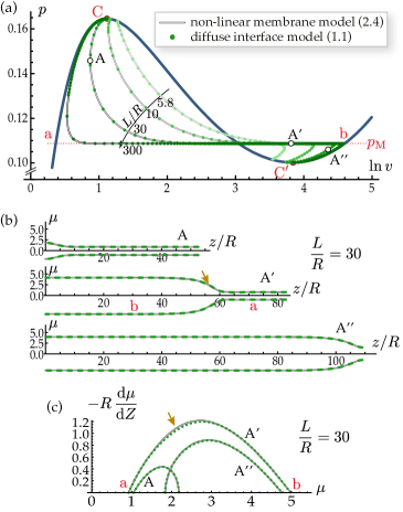
Figure 3: Comparison of the predictions of the non-linear membrane model and of the diffuse interface model, for $F=1.149$. (a) Bifurcation diagrams for different values of the aspect-ratio $L/R$: homogeneous solutions (dark blue curve), bifurcated branches of the membrane model (double-struck black curves) and of the diffuse interface model (green dots); Considère’s points (red dots) and Maxwell’s plateau (dotted red line). Note that we use the logarithm of the scaled volume $v$ on the horizontal axis, so that Maxwell’s equal-area rule does not apply directly. (b) Comparison of the deformed configurations in physical space $(z/R,\mu=r/R)$ for $L/R=30$, for the three configurations labeled $\mathrm{A}$, $\mathrm{A}^{\prime}$ and $\mathrm{A}^{\prime\prime}$ in (a), corresponding to $(v,p)=(2.39,0.146)$, $(45.,0.109)$ and $(77.43,0.106)$ respectively. (c) Same solutions visualized in the phase space: a small discrepancy is visible in the center of the sharp interface (arrow).

In this numerical example, both the membrane and the diffuse interval models use the constitutive law in (4), the standard set of material parameters listed below this equation, and the value of the pulling force $F$ in (6). We limit our attention to solutions that are either homogeneous or comprise a single bulge centered at $Z=0$: recall that the simulation domain $(0,L)$ represents one half of a real balloon.

The equilibrium equations of the membrane model are obtained from the energy (5) by an Euler-Lagrange method, and are solved numerically. These equations of equilibrium and their numerical solution have already been documented in [1], and we refer to this work for details; in our work, the solution branches were calculated using the path-following method from the AUTO-07p library [40]. While [1] used boundary conditions representing rigid plugs, we use instead the natural boundary conditions, namely the axial and radial equilibria $F=\frac{\partial w}{\partial\ell_{z}}\,\frac{z^{\prime}}{\ell_{z}}-p\,e\frac{\ell_{\theta}^{2}}{2}$ and $\mu^{\prime}=0$. These boundary conditions are relevant to the soft boundary device sketched in figure 1b, and are enforced at $Z=L$. At the center of bulge $Z=0$, we impose the symmetry conditions $\mu^{\prime}=0$ and $z=0$.

To solve the diffuse interface model (21) numerically, we first sample the functions $n_{0}(p,\mu)$ and $B_{0}(p,\mu)$ numerically. This tabulation is available as by-product of the analysis of homogeneous solutions from Section 3. Next, the solution branches are generated by solving the boundary value problem (21) using the path-following library AUTO-07p. Alternatively, we tried solving this boundary value problem by the quadrature method described earlier, but it did not work well for the reason already explained.

The bifurcation diagrams are shown in figure 3a. The homogeneous solutions are plotted using the thick, dark blue curve: they are identical for both models, and are also identical to those derived earlier in figure 2d. Bifurcated solutions are shown as black double-struck curves (membrane model) and green dots (diffuse interface model) for different value of $\overline{L}=L/R$. The bifurcation diagram uses the natural logarithm of the scaled volume $v$ on the horizontal axis,

$$v=\frac{1}{L/R}\,\int_{0}^{L}\mu^{2}\,\lambda_{0}(p,\mu)\,\frac{\mathrm{d}Z}{R}\textrm{.}$$ (23)

This is consistent with the definition of the scaled volume $v_{0}$ used in the analysis of homogeneous solutions. For large values of the aspect-ratio $L/R$, the bifurcated branches display a plateau corresponding to Maxwell’s pressure $p_{\mathrm{M}}$.

The diffuse interface model appears to be highly accurate, as its bifurcation diagram is almost identical to that of the membrane model: in the figure, the green dots fall exactly onto the double-struck curves. Given that the diffuse interface model has been derived under an assumption of ‘slow’ axial variations, it could be expected that the models would agree near the bifurcation points (in the neighborhood of the dark blue curve) where the localization is mild. We did not anticipate the good agreement far from the bifurcation point, for configurations featuring relatively sharp interfaces such as that labeled $\mathrm{A}^{\prime}$ in the figure: for this solution, the largest value of the stretch gradient is 1.2, see figure 3c—even though this is not a small number, the diffuse interface model remains remarkably accurate.

Selected deformed configurations are plotted in figure 3b in real space: the predictions of both models are still indistinguishable, even inside the domain boundary. The predictions of the two models are not exactly identical, however: a small difference is visible when these solutions are represented in phase space, see figure 3c; in phase space, the subtle features of the interface are highlighted, while the uniform domains shrink to the points labeled ‘$\mathrm{a}$’ and ‘$\mathrm{b}$’ in the figure.

To sum up, the diffuse interface model reproduces the entire bifurcation diagram of the original membrane model with good accuracy, even for well localized domain boundaries. In the following sections, we show that it is also well suited to linear and non-linear buckling analyses.

5.2 Onset of bulging: linear bifurcation analysis, finite length

We now compare the bifurcation load at the onset of bulging, as predicted by the diffuse interface model on the one hand, and by the membrane model on the other hand. The diffuse interface model yields a simple analytical prediction, that matches that of the membrane model exactly.

The critical load of the diffuse interface model is derived by a classical linear bifurcation analysis as follows. Consider a perturbation to a homogeneous solution $\mu_{0}$, in the form $\mu(Z)=\mu_{0}+\mu_{1}(Z)$. Linearizing the equilibrium equation of the diffuse interface model in (21a) with respect to $\mu_{1}$, we obtain

$$\frac{\partial n_{0}}{\partial\mu}(p,\mu_{0})\,\mu_{1}(Z)+B_{0}(p,\mu_{0})\,\mu_{1}^{\prime\prime}(Z)=0.$$ (24)

The boundary conditions are $\mu_{1}^{\prime}(0)=0$ and $\mu_{1}^{\prime}(L)=0$. The first critical mode $\mu_{1}(Z)=\cos\frac{\pi\,Z}{L}$ corresponds to half a bulge in the simulation domain $(0,L)$. When inserted into the above expression, this yields

$$\frac{\partial n_{0}}{\partial\mu}(p,\mu_{0})=\frac{B_{0}(p,\mu_{0})}{R^{2}}\,\frac{\pi^{2}}{\overline{L}^{2}}\quad\textrm{(diffuse interface model)}\textrm{.}$$ (25)

This equation must be solved together with the axial equilibrium condition for the unperturbed solution (15b), $n_{0}(p,\mu_{0})=0$. For any given value of the aspect-ratio $\overline{L}$, the roots $(p_{\star}(\overline{L}),\mu_{\star}(\overline{L})=\mu_{0}(p_{\star}(\overline{L})))$ of these two equations define the critical parameters where the bifurcation occurs. The corresponding scaled volume can then be reconstructed as $v_{\star}(\overline{L})=v_{0}(p_{\mathrm{\star}}(\overline{L}),\mu_{\star}(\overline{L}))$. The dependence of the critical volume $v_{\star}$ on the aspect-ratio is shown by the green dots in figure 4a.

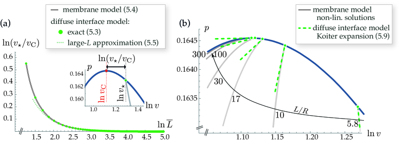
Figure 4: Linear and non-linear bifurcation analyses of the bulging instability based on the diffuse interface model, and comparison with the membrane model. (a) Critical volume $v_{\star}$ at the onset of bulging as a function of the aspect-ratio $\overline{L}=L/R$. The diffuse interface model predicts the bifurcation load exactly (the green dots fall exactly onto the double-struck curve). Inset: bifurcation point shown in the bifurcation diagram as in figure 3a for a particular value $\overline{L}=L/R=5.8$. (b) Initial tangents to the bifurcated branches for different values of the aspect-ratio $\overline{L}=L/R$, as predicted by a weakly non-linear expansion of the membrane model (green dotted lines); comparison with the non-linear branches predicted by the membrane model (double-struck curves).

For comparison, we derive the bifurcation load predicted by the membrane model. The critical load for hard plugs has been obtained by Kyriakides & Chang [1]. Adapting their bifurcation analysis to soft plugs, we obtain the bifurcation condition as

$$\lambda_{0}(p,\mu_{0})\,\frac{(p\,e\,\lambda_{0}(p,\mu_{0})-w_{0,\mu^{2}})\,w_{0,\lambda^{2}}+(w_{0,\lambda\mu}-p\,e\,\mu_{0})^{2}}{w_{0,\lambda}\,w_{0,\lambda^{2}}}=\frac{\pi^{2}}{\overline{L}^{2}}\quad\textrm{(membrane model)}$$ (26)

where commas in subscripts denote partial derivatives of the homogeneous strain energy $w_{0}$ defined in (9), all of which are evaluated at $(\lambda,\mu)=(\lambda_{0}(p,\mu_{0}),\mu_{0})$. Solving this equation together with the axial equilibrium yields $p_{\star}$ and $\mu_{\star}=\mu_{0}(p_{\star})$ as a function of $\overline{L}$, as earlier.

The bifurcation loads of the diffuse interface model (green dots) and of the membrane model (solid dark gray curve) are compared in figure 4a. They agree exactly. This is not surprising as, close to bifurcation, the solutions of the membrane model depart from a uniform solution by an arbitrarily small perturbation, implying that the axial gradients are arbitrarily small: the assumptions underlying the diffuse interface model are satisfied close to the bifurcation point. The diffuse interface model captures exactly the retardation of the onset of buckling in balloons of finite length. Similarly, the critical load predicted by the one-dimensional diffuse interface model for the analysis of necking in solid cylinders has been found in [22] to agree exactly with that based on the three-dimensional analysis of [8].

For large values of the aspect-ratios $\overline{L}$, the bifurcation equation (25) can be simplified by noticing that the left-hand side goes to zero, as the bifurcations takes place closer and closer to the Considère point $(p_{\mathrm{C}},\mu_{\mathrm{C}})$ where the load is maximum, $\frac{\partial n_{0}}{\partial\mu}(p_{\text{C}},\mu_{\text{C}})=0$. Expanding the left-hand side accordingly, one obtains from (25)

$$\mu_{\star}\approx\mu_{\text{C}}+\frac{B_{0}(p_{\text{C}},\mu_{\text{C}})}{R^{2}\,\frac{\partial^{2}n_{0}}{\partial\mu^{2}}(p_{\text{C}},\mu_{\text{C}})}\,\frac{\pi^{2}}{\overline{L}^{2}}\quad\textrm{(diffuse interface model, large $\overline{L}$).}$$ (27)

This yields the dotted curve in figure 4a, which is indeed consistent with the two other curves in the limit $\overline{L}\to\infty$.

5.3 Onset of bulging: weakly non-linear bifurcation analysis, finite length

Following the method of Lyapunov and Koiter [41], an expansion of the bifurcated branch can be found by introducing a small arc-length parameter $\eta$ and expanding $p$ and $\mu$ as

$$\mu =\mu_{0}(p) \;+\; \eta\,\mu_{1}(Z) \;+\; \eta^{2}\,\mu_{2}(Z) \;+\; \mathcal{O}(\eta^{3})$$ (28a)

$$p =p_{\star} \;+\; \eta^{2}\,p_{2} \;+\; \mathcal{O}(\eta^{3}),$$ (28b)

where $\mu_{0}(p)$ denotes the branch of homogeneous solutions satisfying the equilibrium condition $n_{0}(p,\mu_{0}(p))=0$, see (15b), $p_{\star}=p_{\star}(\overline{L})$ is the critical pressure found by the linear stability analysis, $\mu_{1}(Z)=\cos\frac{\pi Z}{L}$ is the linear bifurcation mode, and $\mu_{2}(Z)$ and $p_{2}$ are higher-order corrections. The latter are now determined by inserting this expansion into the non-linear equilibrium (21), and by solving it order by order in $\eta$.

It is actually preferable to work with the weak form of the equilibrium (principle of virtual work), which formally writes $\mathcal{E}_{,\mu}(p,\mu)\cdot[\hat{\mu}]=0$, for any kinematically admissible virtual stretch $\hat{\mu}$. Here, $\mathcal{E}_{,\mu}(p,\mu)$ denotes the first variation of the total potential energy, defined as

$$\mathcal{E}_{,\mu}(p,\mu)\cdot[\hat{\mu}]=\lim_{t\rightarrow 0}\frac{\mathcal{E}(p,\mu+t\,\widehat{\mu})-\mathcal{E}(p,\mu)}{t}\textrm{.}$$

Higher-order variations of the energy are defined similarly.

When the expansion (28) is inserted into the principle of virtual work, one obtains, at order $\eta$, the condition

$$\forall\hat{\mu},\quad\mathcal{E}_{,\mu^{2}}(p_{\star},\mu_{0}(p_{\star}))\cdot[\mu_{1},\hat{\mu}]=0.$$ (29)

We have recovered the bifurcation condition (24), which is automatically satisfied by the linear mode $\mu_{1}(Z)$.

At order $\eta^{2}$ the expansion yields

$$\forall\hat{\mu},\quad\mathcal{E}_{,\mu^{2}}(p_{\star},\mu_{0}(p_{\star}))\cdot[\mu_{2},\hat{\mu}]+\frac{1}{2}\mathcal{E}_{,\mu^{3}}(p_{\star},\mu_{0}(p_{\star}))\cdot[\mu_{1},\mu_{1},\hat{\mu}]=0.$$ (30)

The first term in the left-hand side involves the tangent stiffness operator $\mathcal{E}_{,\mu^{2}}(p_{\star},\mu_{0}(p_{\star}))$ which is known to be singular by the bifurcation condition (29). Therefore a solvability condition must be verified before attempting to solve equation (30) for $\mu_{2}(Z)$; it is derived by replacing $\hat{\mu}$ with $\mu_{1}$ and reads $\mathcal{E}_{,\mu^{3}}(p_{\star},\mu_{0}(p_{\star}))\cdot[\mu_{1},\mu_{1},\mu_{1}]=0$. In the left-hand side, the interactions of the three modes $\mu_{1}$ produces harmonic waves with wave-vector $\pi/L$ and $3\pi/L$, which all cancel out upon integration over the domain $0\leq Z\leq L$: the solvability condition is automatically verified (this is referred to as a symmetric system in bifurcation theory).

Next, equation (30) can be solved for $\mu_{2}$, and the solution reads

$$\mu_{2}(Z)=\mu_{20}+\mu_{21}\cos(\frac{\pi}{L}\,Z)+\mu_{22}\cos(\frac{2\,\pi}{L}\,Z)\textrm{.}$$

The coefficient $\mu_{21}$ remains unspecified at this order (in can be used to re-normalize the arc-length $\eta$), and the other coefficients are found as

$$\mu_{20}=\frac{1}{4}\,\left(\frac{B_{0,\mu}^{\star}}{B_{0}^{\star}}-\frac{n_{0,\mu^{2}}^{\star}}{n_{0,\mu}^{\star}}\right),\qquad\mu_{22}=\frac{1}{12}\,\left(-\frac{3\,B_{0,\mu}^{\star}}{B^{\star}_{0}}+\frac{n_{0,\mu^{2}}^{\star}}{n_{0,\mu}^{\star}}\right),$$

In our notation, any quantity bearing a star is evaluated at the critical point $(p_{\star},\mu_{0}(p_{\star}))$.

Next, the solvability condition at order $\eta^{3}$ yields the coefficient $p_{2}$ as

$$p_{2}=\frac{-3(\lambda_{0,\mu}^{\star}\,n_{0,\mu^{2}}^{\star})^{2}-6\,\lambda_{0}^{\star}\,\lambda_{0,\mu}^{\star}\,n_{0,\mu}^{\star}\,n_{0,\mu^{2}}^{\star}+\lambda_{0}^{\star}\,(6\,\lambda_{0,\mu^{2}}^{\star}\,(n_{0,\mu})^{2}-3\,\lambda_{0}^{\star}\,n_{0,\mu^{3}}^{\star}\,n_{0,\mu}^{\star}+5\,\lambda_{0}^{\star}\,(n_{0,\mu^{2}}^{\star})^{2})}{24\,\lambda_{0}^{\star}\,\left(-\lambda_{0,p}^{\star}\,(n_{0,\mu}^{\star})^{2}+n_{0,\mu}^{\star}\,\left(\lambda_{0,\mu}^{\star}\,n_{0,\mu}^{\star}+\lambda_{0}^{\star}\,n_{0,\mu\,p}^{\star}\right)-\lambda_{0}^{\star}\,n_{0,\mu^{2}}^{\star}\,n_{0,p}^{\star}\right)}\textrm{.}$$

The right-hand side is defined in terms of the properties of the homogeneous solution (§3), and can evaluated numerically for any value of $\overline{L}$: recall that all the quantities in the right-hand side are evaluated at $(p_{\star}(\overline{L}),\mu_{\star}(\overline{L})=\mu_{0}(p_{\star}(\overline{L}))$, where $p_{\star}(\overline{L})$ is the critical load as determined from the linear buckling analysis, see (25).

Finally, an expansion of the volume factor $v$ defined in (23) is obtained as follows. Observe that the integrand defining $v$ is the function $v_{0}(p,\mu)=\mu^{2}\,\lambda_{0}(p,\mu)$: inserting the expansions of $p$ and $\mu$ from (28) into $v_{0}$ and averaging over $Z$, one derives an expansion of the volume factor as $v(p,\mu)=v(p_{\star},\mu_{\star})+v_{2}\,\eta^{2}+\dots$, where the coefficient reads

$$v_{2}=p_{2}\,v_{0,p}^{\star}+\left(\mu_{20}+p_{2}\,\frac{\mathrm{d}\mu_{0}}{\mathrm{d}p}(p_{\star})\right)\,v_{0,\mu}^{\star}+\frac{1}{4}\,v_{0,\mu^{2}}^{\star}.$$

The right-hand side depends on the properties of the homogeneous solutions, and can be evaluated numerically for any given value of the aspect-ratio $\overline{L}$.

When the expansion of $v$ is combined with that of $p$ in (28b), we finally obtain the initial slope of the bifurcated branch as

$$\left(\frac{\mathrm{d}p}{\mathrm{d}v}\right)_{\star}=\frac{p_{2}\,\eta^{2}+\cdots}{v_{2}\,\eta^{2}+\cdots}=\frac{p_{2}}{v_{2}}\textrm{,}$$ (31)

where $p_{2}$ and $v_{2}$ have just been calculated. The corresponding tangents are plotted on figure 4(b) for various values of $\overline{L}$. They agree very well with the bifurcated branches of the non-linear membrane model.

To sum up, the diffuse interface model is amenable to a weakly non-linear analysis which reproduces accurately the solutions of the original, fully non-linear membrane model.

5.4 Onset of localization: weakly non-linear analysis, infinite length

The domain of validity of the weakly non-linear expansion derived in the previous section is more and more limited when the aspect-ratio gets larger, $L/R\to\infty$: in figure 4b, the domain where the tangent (dashed green line) yields a reasonable approximation to the bifurcated branch (black double-struck curve) shrinks when the aspect-ratio increases from $L/R=10$ to $300$. This is because for large values of $L/R$, the extended buckling mode localizes rapidly after bifurcation, a feature not captured by the analysis of the previous section. Here, we derive a different weakly non-linear solution of the diffuse interface model, assuming that the cylinder is infinitely long, $L/R=\infty$. This solution captures the quick localization of the bulges; it is similar to that derived Fu et al. [31] based on the full membrane model but its derivation is somewhat simpler.

In the limit $L/R\to\infty$, the bifurcation takes place at the Considère point $(\mu_{\mathrm{C}},p_{\mathrm{C}})$, where the pressure attains its maximum (the other bifurcation taking place at the minimum pressure $p_{\mathrm{C^{\prime}}}$, which can be treated similarly). Accordingly, the weakly bulged solution satisfies $p\approx p_{\mathrm{C}}$ and $\mu(Z)\approx\mu_{\mathrm{C}}$, and the potential $G_{0}$ can be expanded as

$$G_{0}(p,\mu)=G_{0}^{\mathrm{C}}+G_{0,p}^{\mathrm{C}}\,(p-p_{\mathrm{C}})+G_{0,\mu}^{\mathrm{C}}\,(\mu-\mu_{\mathrm{C}})\cdots\\ {}+\frac{G_{0,p^{2}}^{\mathrm{C}}}{2}\,(p-p_{\mathrm{C}})^{2}+G_{0,p\mu}^{\mathrm{C}}\,(p-p_{\mathrm{C}})\,(\mu-\mu_{\mathrm{C}})+\frac{G_{0,\mu^{2}}^{\mathrm{C}}}{2}\,(\mu-\mu_{\mathrm{C}})^{2}+\frac{G_{0,\mu^{3}}^{\mathrm{C}}}{6}\,(\mu-\mu_{\mathrm{C}})^{3}+\cdots$$ (32)

The arguments appearing in subscript after a comma denote a partial derivative, while a superscript ‘$\mathrm{C}$’ means that the function is evaluated at Considère’s point $(p_{\mathrm{C}},\mu_{\mathrm{C}})$. The values of all the coefficients $G_{0}^{\mathrm{C}}$, $G_{0,p}^{\mathrm{C}}$, etc. are available from the analysis of homogeneous solutions (§3).

In the right-hand side above, we can discard the terms that do not depend on $\mu$, as well as the terms containing $G_{0,\mu}^{\mathrm{C}}$ which cancels by equation (15b), and that containing $G_{0,\mu^{2}}^{\mathrm{C}}$ which cancels a the maximum pressure $p_{\mathrm{C}}$. Accordingly, the energy (1) can be approximated as

$$\mathcal{E}\approx\int_{-\infty}^{+\infty}\left[\mathrm{Cte}(p)+G_{0,p\mu}^{\mathrm{C}}\,(p-p_{\mathrm{C}})\,(\mu-\mu_{\mathrm{C}})+\frac{G_{0,\mu^{3}}^{\mathrm{C}}}{6}\,(\mu-\mu_{\mathrm{C}})^{3}+\frac{1}{2}\,B_{0}^{\mathrm{C}}\,\left(\frac{\mathrm{d}\mu}{\mathrm{d}Z}\right)^{2}\right]\,\mathrm{d}Z\textrm{.}$$ (33)

The signs of the coefficients appearing in the integrand are important: for our particular constitutive law and using the results of Section 3, their numerical value is

$$G_{0,p\mu}^{\mathrm{C}}=\frac{\partial^{2}G_{0}}{\partial p\,\partial\mu}(p_{\mathrm{C}},\mu_{\mathrm{C}})=-9.366,\quad G_{0,\mu^{3}}^{\mathrm{C}}=\frac{\partial^{3}G_{0}}{\partial\mu^{3}}(p_{\mathrm{C}},\mu_{\mathrm{C}})=-3.413,\quad B_{0}^{\mathrm{C}}=B_{0}(p_{\mathrm{C}},\mu_{\mathrm{C}})=0.8956\textrm{.}$$

A balance argument on the three last term in the integrand above suggests the change of variable

$$\mu(Z)=\mu_{\mathrm{C}}+(p_{\mathrm{C}}-p)^{1/2}\,\mu^{{\dagger}}\,\overline{\mu}(\overline{Z})$$ (34a)

where

$$\mu^{{\dagger}}=\left(\frac{2\,|G_{0,p\mu}^{\mathrm{C}}|}{|G_{0,\mu^{3}}^{\mathrm{C}}|}\right)^{1/2},\quad\overline{Z}=\left(\frac{2\,|G_{0,p\mu}^{\mathrm{C}}|\,|G_{0,\mu^{3}}^{\mathrm{C}}|}{(B_{0}^{\mathrm{C}})^{2}}\,(p_{\mathrm{C}}-p)\right)^{1/4}\,Z\textrm{.}$$ (34b)

In terms of the rescaled variables, the energy expansion (33) writes

$$\overline{\mathcal{E}}=\frac{1}{2}\int_{-\infty}^{+\infty}\left[\overline{\mu}(\overline{Z})-\frac{\overline{\mu}^{3}(\overline{Z})}{3}+\left(\frac{\mathrm{d}\overline{\mu}}{\mathrm{d}\overline{Z}}\right)^{2}\right]\,\mathrm{d}\overline{Z},$$

after dropping the term $G_{0}(p,\mu_{\mathrm{C}})$ that is independent of $\mu$, and rescaling the energy using a numerical constant. The weakly non-linear solutions are the stationary points $\overline{\mu}(\overline{Z})$ of this energy functional. They can be analyzed based on the analogy with a mass moving in a potential $U(\overline{\mu})=-\frac{\overline{\mu}}{2}+\frac{\overline{\mu}^{3}}{6}$, when $\overline{Z}$ is viewed as a time variable. A first type of solutions are those corresponding to the equilibria in the effective potential $U(\overline{\mu})$, namely $\overline{\mu}(\overline{Z})=\pm 1$: they yield an expansion of the branch of homogeneous solutions near the point of maximum pressure, as can be checked. A second type of solution corresponds to a soliton, i.e. to a non-constant but bounded solution; it can be derived by a quadrature method, using the conservation of the total mechanical energy of the mass in the effective potential. The result is

$$\overline{\mu}(\overline{Z})=-1+\frac{3}{\cosh^{2}\frac{\overline{Z}-\overline{Z}_{0}}{2}}\textrm{.}$$ (35)

This solution represents a weakly localized bulge centered about $\overline{Z}_{0}$. It is identical to that derived by Fu et al. [31] based on the full membrane model. The soliton solution (35) is plotted in figure 5b–c, and compared to the non-linear solution of the diffuse interface model: the weakly non-linear solution and the full non-linear solution agree asymptotically close to the bifurcation point, as expected.

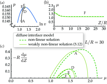
Figure 5: Comparison of the analytical weakly non-linear solutions (35) and the numerical non-linear solutions of the diffuse interface model, for an aspect-ratio $L/R=30$. The simulation domain represents one half of a balloon having a single bulge in the center. (a) Position of a few selected configurations in the phase diagram; point $\mathrm{A}$ is the same configuration as in figure 3. (b) Comparison close to the bifurcation point. (c) Comparison for different bulging amplitudes in phase space: the weakly non-linear solution is asymptotically exact for small bulging amplitudes.

Unlike the weakly non-linear solution from the previous section, this solution captures the rapid localization of the bulge past the bifurcation point: from (34b), the width of the interface is $Z\sim(p-p_{\mathrm{C}})^{-1/4}$ near bifurcation.

To derive the weakly non-linear solution, we have retained some terms in the expansion of the energy (33), and omitted others such as $\frac{1}{2}\,G_{0,\mu p^{2}}^{\mathrm{C}}\,(\mu-\mu_{\mathrm{C}})\,(p-p_{\mathrm{C}})^{2}$ or $\frac{1}{2}\,B_{0,p}^{\mathrm{C}}\,(p-p_{\mathrm{C}})\,{\mu^{\prime}}^{2}$. This can be justified a posteriori, based on the scaling laws of the weakly non-linear solution: the scaling assumptions $(\mu-\mu_{\mathrm{C}})\sim(p_{\mathrm{C}}-p)^{1/2}$ and $Z\sim(p_{\mathrm{C}}-p)^{-1/4}$ not only make the last three terms in (33) balanced (which is by design), they also make the other terms negligible, as can be checked. The expansion (33) is therefore consistent.

6 Conclusion and final remarks

We have proposed a diffuse interface model for the analysis of the formation, localization and propagation of bulges in cylindrical rubber balloons. The model has been derived from the non-linear membrane theory, and is asymptotically exact in the limit where the strain gradient $\frac{\mathrm{d}\mu}{\mathrm{d}Z}$ is small compared to $1/R$. Analytical and numerical solutions to the diffuse interface model have been obtained, showing good agreement with the predictions of the original non-linear membrane model, both at the onset of localization and for well-localized solutions: in practice, the diffuse interface model remains accurate well beyond its domain of strict mathematical validity, i.e. even for relative large gradients such as those found at the boundary between a bulged and a non-bulged domain. Hopefully, our work will shed new light on the classical problem of bulging in elastic balloons, and will help highlighting its tight connection with the theory of phase transitions.

The model handles finite strain: only the strain gradients are assumed to be small. The elastic response of the material under finite strain gets reflected into the diffuse interface model through the non-linear potential $G_{0}(p,\mu)$ and the non-linear strain gradient modulus $B_{0}(p,\mu)$. Thanks to this feature, the predictions of the model are exact as far as linear bifurcation analyses are concerned, and remain accurate even well into the post-bifurcation regime. By contrast, expansion methods underlying bifurcation analyses typically assume that the solution is close to a homogeneous solution, and have a much narrower domain of applicability.

A simple expression for the coefficient $B_{0}(p,\mu)$ of the strain gradient term has been established, see (20b). Remarkably, this coefficient is directly proportional to the pre-stress $\boldsymbol{\Sigma}_{0}$ in the homogeneous solution, see (19). The same observation has been made concerning the strain-gradient model applicable to necking in a hyperelastic cylinder [22]. In both cases, the contribution of the strain gradient to the elastic energy occurs through a ‘geometric rigidity effect’ — the vibration of a string under tension is another example of this geometric rigidity effect, whereby the pre-stress brings in an effective elastic stiffness.

The consistency of our results with those of Audoly & Hutchinson [22] for a solid cylinder can be checked as follows. In (20a), we have derived the contribution of the strain gradient to the energy of a balloon using dimensionless quantities. In terms of the original (non-scaled) quantities, it can be rewritten as $\frac{1}{2}\int_{0}^{L}B_{0}^{*}\,\mu^{\prime 2}(Z)\,\mathrm{d}Z$, where the non-scaled modulus is found from (20b) as $B_{0}^{*}=(2\pi\,R\,H)\,R^{2}\,\frac{1}{\lambda}\frac{\partial{w}_{0}^{*}}{\partial\lambda}$, after restoring the initial area that had been scaled out. Identifying $I=(2\pi\,R\,H)\,R^{2}$ as the geometric moment of inertia of the annular cross-section in reference configuration, the contribution of the strain gradient to the energy can therefore be written as $\frac{1}{2}\int_{0}^{L}I\,\frac{1}{\lambda}\frac{\partial{w}_{0}^{*}}{\partial\lambda}\,\mu^{\prime 2}(Z)\,\mathrm{d}Z$ in an axisymmetric membrane. In fact, this holds for a solid cylinder as well, as can be checked by combining equations 2.28, 2.13 and 2.8 from [22].

In the future, the following extensions of the model could be considered. While we have only been concerned with bifurcations in this paper, one could analyze the stability of the solutions based on the diffuse interface model as well: presumably, this would confirm the stability results obtained previously from the non-linear membrane model. Different boundary conditions than the natural boundary conditions could be used at the ends of the balloons: a hard plug can be enforced by the boundary condition $\mu=1$, while a rounded elastic cap can be prescribed through a non-cylindrical reference configuration $R(Z)$; if, however, the prescribed initial profile $R$ varies quickly with $Z$, there may be a conflict with our asymptotic procedure that assumes slow variations, and the diffuse interface model may not be able to account accurately for such boundary conditions. A coupling with an electrical field could also be introduced, as is relevant to the actuation of balloons made of dielectric elastomers [42, 43, 44]; we believe that a natural extension of our asymptotic expansion can be derived for dielectric balloons. In future work, we also hope to apply our asymptotic reduction method to other localization phenomena occurring in slender structures, such as the Plateau-Rayleigh instability in soft elastic rods with surface tension [45], and the localized kinks in tape springs [12, 13].

We would like to thank John Hutchinson for drawing our attention to the absence of a strain gradient model for the analysis of bulging in balloons, and for providing useful feedback on the manuscript.

Appendix A Elimination of $\lambda(Z)$ from the diffuse interface model

This appendix provides details on the elimination of the unknown $\lambda(Z)$ from the intermediate form (19) of the energy, leading to the final form (20).

As the approximation of the energy (19) contains no derivative of the axial stretch $\lambda$, optimizing with respect with the $\lambda$ variable yields an algebraic (i.e. non-differential) problem for $\lambda(Z)$

$$\frac{\partial g_{0}}{\partial\lambda}(p,\lambda(Z),\mu(Z))+\frac{\partial\boldsymbol{\Sigma}_{0}}{\partial\lambda}(\lambda(Z),\mu(Z))\cdot\mathbf{E}_{1}(\mu^{\prime}(Z))+\mathcal{O}(\varepsilon^{4})=0.$$ (36)

The first term is of order $\varepsilon^{0}=1$, the following term is of order $\varepsilon^{2}$ by (17h), and we have omitted terms of order $\varepsilon^{4}$ and higher.

Let us solve (36) order by order for $\lambda$. At dominant order $\varepsilon^{0}=1$, $\lambda(Z)$ is a solution of $\frac{\partial g_{0}}{\partial\lambda}(p,\lambda,\mu(Z))=0$, which we identify as the equilibrium condition (12a) applicable to homogeneous solutions. In (13), the solution to this equation has be=en introduced as $\lambda(Z)=\lambda_{0}(p,\mu(Z))$, i.e.

$$\lambda(Z)=\lambda_{0}(p,\mu(Z))+\mathcal{O}(\varepsilon^{2}).$$

To order $\varepsilon^{2}$, the solution of equation (36) is found as

$$\lambda(Z)=\lambda_{0}(p,\mu(Z))+\lambda_{[2]}(Z)+\mathcal{O}(\varepsilon^{4}),$$ (37)

where $\lambda_{[2]}=-\left(\frac{\partial\boldsymbol{\Sigma}_{0}}{\partial\lambda}\cdot\mathbf{E}_{1}(\mu^{\prime})\right)/\frac{\partial^{2}g_{0}}{\partial\lambda^{2}}$ is a correction of order $\varepsilon^{2}$, arising from the strain correction $\mathbf{E}_{1}(\mu^{\prime})=\mathcal{O}(\varepsilon^{2})$ (the expression of $\lambda_{[2]}$ is given for the sake of completeness but is not needed in the following).

Inserting the expansion (37) for $\lambda(Z)$ into (19) and expanding in series, we find

$$\mathcal{E}=\int\left[G_{0}(p,\mu)+\frac{\partial g_{0}}{\partial\lambda}(p,\lambda_{0},\mu)\,\lambda_{[2]}\right]\,\mathrm{d}Z+\int\boldsymbol{\Sigma}_{0}(\lambda_{0},\mu)\cdot\mathbf{E}_{1}(\mu^{\prime})\,\mathrm{d}Z+\mathcal{O}(L\,\varepsilon^{4}),$$

where we use $\lambda_{0}$ as a shorthand for $\lambda_{0}(p,\mu(Z))$. As the second term in the bracket vanishes by (13), we are left with

$$\mathcal{E}=\int G_{0}(p,\mu)\,\mathrm{d}Z+\int\boldsymbol{\Sigma}_{0}(\lambda_{0},\mu)\cdot\mathbf{E}_{1}(\mu^{\prime})\,\mathrm{d}Z+\mathcal{O}(L\,\varepsilon^{4}).$$

Inserting the explicit expressions of $\boldsymbol{\Sigma}_{0}$ and $\mathbf{E}_{1}$ from (10) and (17g), one obtains the expressions announced in (20).

References

- Kyriakides and Chang [1991] S. Kyriakides, Y.-C. Chang, The initiation and propagation of a localized instability in an inflated elastic tube, International Journal of Solids and Structures 27 (9) (1991) 1085–1111.
- Chater and Hutchinson [1984] E. Chater, J. W. Hutchinson, On the propagation of bulges and buckles, Journal of Applied Mechanics 51 (2) (1984) 269–277.
- Ericksen [1975] J. L. Ericksen, Equilirbium of bars, Journal of Elasticity 5 (1975) 191.
- Bhattacharya [2004] S. Bhattacharya, Microstructure of martensite, Oxford Series on materials modelling, Oxford University Press, 2004.
- Fu and Freidin [2004] Y. Fu, A. Freidin, Characterization and stability of two-phase piecewise-homogeneous deformations, Proc. R. Soc. A 460 (2004) 2065.
- Bridgman [1952] P. W. Bridgman, Studies in large plastic flow and fracture, Metallurgy and metallurgical engineering series, McGraw-Hill, New York, 1952.
- Barenblatt [1974] G. I. Barenblatt, Neck propagation in polymers, Rheologica Acta 13 (1974) 924–933.
- Hutchinson and Miles [1974] J. W. Hutchinson, J. P. Miles, Bifurcation analysis of the onset of necking in an elastic/plastic cylinder under uniaxial tension, Journal of the Mechanics and Physics of Solids 22 (1974) 61–71.
- Wadee et al. [2004] M. A. Wadee, G. W. Hunt, M. A. Peletier, Kink band instabilities in layered structures, Journal of the Mechanics and Physics of Solids 52 (2004) 1071–1091.
- Fu and Zhang [2006] Y. Fu, Y. Zhang, Continuum-mechanical modelling of kink-band formation in fibre-reinforced composites, International Journal of Solids and Structures 43 (2006) 3306.
- Power and Kyriakides [1994] T. L. Power, S. Kyriakides, Localization and propagation of instabilities in long shallow panels under external pressure, Journal of Applied Mechanics 61 (1994) 755–763.
- Seffen and Pellegrino [1999] K. A. Seffen, S. Pellegrino, Deployment dynamics of tape springs, Proceedings of the Royal Society of London. Series A: Mathematical, Physical and Engineering Sciences 455 (1983) (1999) 1003–1048.
- Seffen et al. [2000] K. A. Seffen, Z. You, S. Pellegrino, Folding and deployment of curved tape springs, International Journal of Mechanical Sciences 42 (10) (2000) 2055–2073.
- Triantafyllidis and Bardenhagen [1996] N. Triantafyllidis, S. Bardenhagen, The influence of scale size on the stability of periodic solids and the role of associated higher order gradient continuum models, Journal of the Mechanics and Physics of Solids 44 (1996) 1891–1928.
- Knowles and Sternberg [1978] J. Knowles, E. Sternberg, On the failure ot ellipticity and the emergence of discontinuous deformation gradients in plane finite elastostatics, journal of Elasticity 4 (1978) 329.
- Triantafyllidis and Aifantis [1986] N. Triantafyllidis, E. C. Aifantis, A gradient approach to localization of deformation. I. Hyperelastic materials, Journal of Elasticity 16 (1986) 225–237.
- Triantafyllidis and Bardenhagen [1993] N. Triantafyllidis, S. Bardenhagen, On higher order gradient continuum theories in 1-D nonlinear elasticity. Derivation from and comparison to the corresponding discrete models, Journal of Elasticity 33 (3) (1993) 259–293.
- Bardenhagen and Triantafyllidis [1994] S. Bardenhagen, N. Triantafyllidis, Derivation of higher order gradient continuum theories in 2,3-d non-linear elasticity from periodic lattice models, J. Mech. Phys. Solids 42 (1994) 111–139.
- Abdoul-Anziz and Seppecher [2018] H. Abdoul-Anziz, P. Seppecher, Strain gradient and generalized continua obtained by homogenizing frame lattices, Mathematics and Mechanics of Complex Systems .
- Bacigalupo et al. [2017] A. Bacigalupo, M. Paggi, F. Dal Corso, D. Bigoni, Identification of higher-order continua equivalent to a Cauchy elastic composite, Mechanics Research Communications .
- Mielke [1991] A. Mielke, Hamiltonian and Lagrangian flows on center manifolds, with application to elliptic variational problems, vol. 1489 of Lecture notes in mathematics, Springer-Verlag, Berlin, 1991.
- Audoly and Hutchinson [2016] B. Audoly, J. W. Hutchinson, Analysis of necking based on a one-dimensional model, Journal of Mechanics Physics of Solids 97 (2016) 68–91.
- Kyriakides and Chang [1990] S. Kyriakides, Y.-C. Chang, On the inflation of a long elastic tube in the presence of axial load, International Journal of Solids and Structures 26 (1990) 975.
- van der Waals [1894] J. D. van der Waals, Thermodynamische Theorie der Kapillarität unter Voraussetzung stetiger Dichteänderung., Z. Phys. Chem. 13 (1894) 657–725.
- Müller and Strehlow [2004] A. Müller, P. Strehlow, Rubber and Rubber Balloons, Springer, 2004.
- Corneliussen and Shield [1961] A. Corneliussen, R. T. Shield, Finite Deformation of Elastic Membranes with Application to the Stability of an Inflated and Extended Tube, Arch. Rational Mech. Anal. 7 (1961) 273.
- Shield [1972] R. T. Shield, On the stability of finitely deformed elastic membranes, Part II: stability of inflated cylindrical and spherical membranes., J. Appl. Math. Phys. 23.
- Haughton and Odgen [1979] D. M. Haughton, R. W. Odgen, Bifurcation of inflated circular cylinders of elastic material under axial loading, part i: membrane theory for thin-walled tubes, Journal of the Mechanics and Physics of Solids 27 (1979) 179.
- Yin [1977] W.-L. Yin, Non-uniform inflation of a cylindrical elastic membrane and direct determination of the strain energy function, Journal of Elasticity 7 (3) (1977) 265–282.
- Chen [1997] Y.-C. Chen, Stability and bifurcation of finite deformations of elastic cylindrical membranes, part I: Stability analysis, International Journal of Solids and Structures 34 (1997) 1735.
- Fu et al. [2008] Y. B. Fu, S. P. Pearce, K. K. Liu, Post-bifurcation analysis of a thin-walled hyperelastic tube under inflation, International Journal of Non-Linear Mechanics 43 (8) (2008) 697–706.
- Fu and Xie [2010] Y. B. Fu, Y. X. Xie, Stability of localized bulging in inflated membrane tubes under volume control, International Journal of Engineering Science 48 (2010) 1242–1252.
- Pearce and Fu [2010] S. P. Pearce, Y. B. Fu, Characterization and stability of localized bulging/necking in inflated membrane tubes, IMA Journal of Applied Mathematics 75 (2010) 581–602.
- Fu and Xie [2012] Y. B. Fu, Y. X. Xie, Effects of imperfections on localized bulging in inflated membrane tubes, Philosophical Transactions of the Royal Society A: Mathematical, Physical and Engineering Sciences 370 (2012) 1896–1911.
- Coleman and Newman [1988] B. D. Coleman, D. C. Newman, On the Rheology of Cold Drawing. I. Elastic Materials, Journal of Polymer Science: Part B: Polymer Physics 26 (1988) 1801.
- Dai and Cai [2006] H.-H. Dai, Z. Cai, Phase transitions in a slender cylinder composed of an incompressible elastic material. I. Asymptotic model equation, Proc. R. Soc. A 462 (2006) 75–95.
- Dai and Wang [2009] H.-H. Dai, J. Wang, An analytical study on the geometrical size effect on phase transitions in a slender compressible hyperelastic cylinder, International Journal of Non-Linear Mechanics 44 (2009) 219–229.
- Ogden [1972] R. W. Ogden, Large deformation isotropic elasticity-on the correlation of theory and experiment for incompressible rubber-like solids, Proceedings of the Royal Society A: Mathematical, Physical and Engineering Science 326 (1972) 565–584.
- Considère [1885] A. Considère, Mémoire sur l’emploi du fer et de l’acier dans les constructions, Annales des Ponts et Chaussées, Série 6 9 (1885) 574–775.
- Doedel et al. [2007] E. J. Doedel, A. R. Champneys, T. F. Fairgrieve, Y. A. Kuznetsov, B. Sandstede, X. J. Wang, AUTO-07p: continuation and bifurcation software for ordinary differential equations, See http://indy.cs.concordia.ca/auto/, 2007.
- Koiter [1965] W. T. Koiter, On the stability of elastic equilibrium, Ph.D. thesis, Delft, Holland, 1965.
- Lu and Suo [2012] T.-Q. Lu, Z. Suo, Large conversion of energy in dielectric elastomers by electromechanical phase transition, Acta Mechanica sinica 28 (4) (2012) 1106–1114.
- Lu et al. [2015] T. Lu, L. An, J. Li, C. Yuan, T. J. Wang, Electro-mechanical coupling bifurcation and bulging propagation in a cylindrical dielectric elastomer tube, Journal of the Mechanics and Physics of Solids 85 (2015) 160–175.
- An et al. [2015] L. An, F. Wang, S. Cheng, T. Lu, T. J. Wang, Experimental investigation of the electromechanical phase transition in a dielectric elastomer tube, Smart Materials and Structures 24 (3) (2015) 035006.
- Xuan and Biggins [2017] C. Xuan, J. Biggins, Plateau-Rayleigh instability in solids is a simple phase separation, Physical Reivew E 95 (2017) 053106.