Minimal Geometric Deformation decoupling in $2+1$ dimensional space–times

Abstract

We study the Minimal Geometric Deformation decoupling in $2+1$ dimensional space–times and implement it as a tool for obtaining anisotropic solutions from isotropic geometries. Interestingly, both the isotropic and the anisotropic sector fulfill Einstein field equations in contrast to the cases studied in $3+1$ dimensions. In particular, new anisotropic solutions are obtained from the well known static BTZ solution.

I Introduction

It is well known that the Minimal Geometric Deformation (MGD) decoupling, originally proposed ovalle2008 in the context of the Randall–Sundrum brane–world randall1999a ; randall1999b , has been a powerful tool to investigate self–gravitating distributions in the brane–world scenario ovalle2009 ; ovalle2010 ; casadio2012 ; ovalle2013 ; ovalle2013a ; casadio2014 as well as to find new black hole solutions in a more general context casadio2015 ; ovalle2016 (for some recent appplications see for instance ovalle2015 ; casadio2015b ; cavalcanti2016 ; casadio2016a ; ovalle2017 ; rocha2017a ; rocha2017b ; casadio2017a ; ovalle2018 ; estrada2018 ; ovalle2018a ; lasheras2018 ; gabbanelli2018 ; sharif2018 ; fernandez2018 ; fernandez2018b ). In recent years, the use of the MGD–decoupling as a method to obtain new and relevant solutions of the Einstein field equations has increased considerably ovalle2017 ; ovalle2018 ; estrada2018 ; ovalle2018a ; lasheras2018 ; gabbanelli2018 ; sharif2018 . In particular, it is interesting to note that local anisotropy can be induced in well known spherically symmetric isotropic solutions of self–gravitating objects, leading to more realistic interior solutions of stellar systems.

Inspired by the success of the method in $3+1$ dimensional space–times, it would be worth considering the application of the MGD- decoupling method in the lowest dimension in which the Einstein theory makes sense, i. e., three dimensional space–times. Although, as stated by Staruszkiewicz in his pioneering paper staruszkiewicz1963 “three-dimensional gravitation theory is a theory without a field of gravitation; where no matter is present, space is flat”, solutions of the Einstein field equations in $2+1$ dimensional space–times coupled to matter content have been considered as a testing ground to study some aspects shared with their $3+1$ dimensional counterparts with emphasis given to point particle solutions, perfect fluids, cosmological spacetimes, dilatons, inflatons, stringy solutions, etc. (for a recent and very exhaustive review on 2+1 exact solutions, see Garciabook2017 ).

In particular, some properties of $3+1$-dimensional black holes such as horizons, Hawking radiation and black hole thermodynamics, are also present in three-dimensional gravity which is simpler to deal with. Such is the case of the celebrated BTZ btz black hole solution, which shares many of the features of the Kerr black hole, for instance the presence of event and inner horizons, an ergosphere and a nonvanishing Hawking temperature.
For these reasons, in this work we shall study the MGD-decoupling method in three-dimensional space–times and obtain anisotropic solutions from the static BTZ solution. The work is organized as follows. In the next section we review the main features of the Einstein equations coupled to matter sources in three–dimensional space–times. Next, we implement the MGD-decoupling method applied to a circularly symmetric system containing a perfect fluid in section III. Section IV is devoted to obtaining anisotropic solutions from the static BTZ geometry. We summarize our conclusions in section V.

II Einstein equations

Let us consider the Einsteins field equations

$$R_{\mu\nu}-\frac{1}{2}Rg_{\mu\nu}=-\kappa^{2}T_{\mu\nu}^{tot},$$ (1)

and assume that the total energy-momentum tensor is given by

$$T_{\mu\nu}^{(tot)}=T_{\mu\nu}^{(m)}+\alpha\theta_{\mu\nu},$$ (2)

where $T^{\mu}_{\nu}=diag(-\rho,p,p)$ is the matter energy momentum for a perfect fluid and $\theta_{\mu\nu}$ is an additional source coupled with the perfect fluid by the constant $\alpha$. Since the Einstein tensor is divergence free, the total energy momentum tensor $T_{\mu\nu}^{(tot)}$ satisfies

$$\nabla_{\mu}T^{(tot)\mu\nu}=0.$$ (3)

In Schwarzschild like-coordinates, the circularly symmetric line element reads

$$ds^{2}=e^{\nu}dt^{2}-e^{\lambda}dr^{2}-r^{2}d\phi^{2},$$ (4)

where $\nu$ and $\lambda$ are functions of the radial coordinate $r$ only. Considering the metric (4) as a solution of the Einstein equations, we obtain

$$8\pi\tilde{\rho} = \frac{e^{-\lambda}\lambda^{\prime}}{2r}$$ (5)

$$8\pi\tilde{p}_{r} = \frac{e^{-\lambda}\nu^{\prime}}{2r}$$ (6)

$$8\pi\tilde{p}_{\perp} = -\frac{e^{-\lambda}}{4}\left(\nu^{\prime}\left(\lambda^{\prime}-\nu^{\prime}\right)-2\nu^{\prime\prime}\right),$$ (7)

where the prime denotes derivation respect to the radial coordinate and we have defined

$$\tilde{\rho} = \rho+\alpha\theta^{0}_{0}$$ (8)

$$\tilde{p}_{r} = p-\alpha\theta^{1}_{1}$$ (9)

$$\tilde{p}_{\perp} = p-\alpha\theta^{2}_{2}.$$ (10)

The conservation equation (3) reads

$$p^{\prime}+\frac{\nu^{\prime}}{2}(\rho+p)-\alpha(\theta^{1}_{1})^{\prime}+\frac{\nu^{\prime}\alpha}{2}(\theta^{0}_{0}-\theta^{1}_{1})+\frac{\alpha}{r}(\theta^{2}_{2}-\theta^{1}_{1})=0,$$ (11)

which is a linear combination of Eqs. (5), (6) and (7). Note that Eqs. (5), (6) and (7) correspond to the Einstein field equations for an anisotropic fluid. In this sense, the source $\theta_{\mu\nu}$ generate anisotropy in the original system controlled by the parameter $\alpha$, which disappears when $\alpha\to 0$, as can be easily checked. Note that we have to solve for Eqs. (5), (6), (7) and (11) but we deal with five unknows functions, $\{\nu,\lambda,\tilde{\rho},\tilde{p}_{r},\tilde{p}_{\perp}\}$. A conventional way to decrease the degrees of freedom to solve the system of differential equations considered is providing an ansatz which in general is an equation of state relating the components of the energy–momentum tensor. However, in this work, we shall obtain solutions by the MGD–decoupling method, as explained further below.

III Minimal geometric deformation

In this section we introduce the MGD-decoupling method for $2+1$ dimensional space–times. Let us implement the following “geometric deformation” on the radial metric component $g^{rr}$

$$e^{-\lambda}=\mu(r)+\alpha f(r),$$ (12)

where $\alpha$ is the decoupling parameter and $f(r)$ is the generic deformation undergone by the radial metric component, $\mu(r)$. After replacing (12) in Einstein equations (5), (6) and (7), we can separate the system of equations in two sets as follows. One set is obtained by setting $\alpha=0$ and corresponds to a perfect fluid

$$16\pi r\rho = -\mu^{\prime}$$ (13)

$$16\pi p = \frac{\mu\nu^{\prime}}{r}$$ (14)

$$32\pi p = \mu^{\prime}\nu^{\prime}+2\mu\nu^{\prime\prime}+\mu\nu^{\prime 2},$$ (15)

with conservation equation given by

$$p^{\prime}+\frac{\nu^{\prime}}{2}(\rho+p)=0,$$ (16)

which is a linear combination of Eqs. (13), (14) and (15). The other set of equations corresponds to the source $\theta_{\mu\nu}$

$$16\pi r\theta^{0}_{0} = -f^{\prime}$$ (17)

$$-16\pi\theta^{1}_{1} = \frac{f\nu^{\prime}}{r}$$ (18)

$$-32\pi\theta^{2}_{2} = f^{\prime}\nu^{\prime}+2f\nu^{\prime\prime}+f\nu^{\prime 2},$$ (19)

with conservation

$$(\theta^{1}_{1})^{\prime}-\frac{\nu^{\prime}}{2}(\theta^{0}_{0}-\theta^{1}_{1})-\frac{1}{r}(\theta^{2}_{2}-\theta^{1}_{1})=0.$$ (20)

As in the previous case, Eq. (20) is the linear combination of Eqs. (17), (18) and (19). Note that unlike the $3+1$ dimensional cases studied in ovalle2017 ; ovalle2018 ; ovalle2018a ; lasheras2018 ; estrada2018 both the equations of the isotropic (perfect fluid) and anisotropic ($\theta_{\mu\nu}$) sector are Einstein equations. In this sense, the Einstein tensor $G_{\mu\nu}$ of the new solution turns out to be the linear combination of two Einstein tensor each one fulfilling Einstein field equations. More precisely, if $G^{(m)}_{\mu\nu}=-\kappa^{2}T^{m}_{\mu\nu}$ stands for the isotropic sector, and $\tilde{G}_{\mu\nu}=-\kappa^{2}\alpha\theta_{\mu\nu}$ for the anisotropic one, the Einstein tensor of the new solution is simply given by $G_{\mu\nu}=G^{(m)}_{\mu\nu}+\tilde{G}_{\mu\nu}$. The above result can be naturally extended for arbitrary number of sources, namely, given the Einstein Field Equations for a collection of sources they can be transformed into a collection of Einstein’s equations, one for each source. Even more, given a source $T^{(tot)}_{\mu\nu}=T_{\mu\nu}^{(m)}+\sum\limits_{i}\alpha_{i}\theta^{(i)}_{\mu\nu}$, with $i\geq 1$ and $\nabla_{\mu}T^{\mu\nu}=\nabla_{\mu}\theta^{(1)\mu\nu}=\cdots=\nabla_{\mu}\theta^{(n)\mu\nu}=0$, the Einstein tensor associated with $T^{(tot)}_{\mu\nu}$ can be decomposed as $G_{\mu\nu}=G^{(m)}_{\mu\nu}+G^{(1)}_{\mu\nu}+\cdots G^{(n)}_{\mu\nu}$ from where

$$G^{(m)}_{\mu\nu} = -\kappa^{2}T^{(m)}_{\mu\nu}$$

$$G^{(1)}_{\mu\nu} = -\kappa^{2}\alpha_{1}\theta^{(1)}_{\mu\nu}$$

$$\vdots \vdots$$

$$G^{(n)}_{\mu\nu} = -\kappa^{2}\alpha_{n}\theta^{(n)}_{\mu\nu}.$$ (21)

This fact is remarkable because in $3+1$ space–times the anisotropic system does not fulfil Einstein but “quasi Einstein” field equations ovalle2017 ; ovalle2018 ; ovalle2018a as a consequence of a missed $-\frac{1}{r^{2}}$ term which avoid the matching with standard Einstein equations. Even more, in $3+1$ dimensions it is shown that, despite this “quasi Einstein” behaviour for the equations, the conservation can be written as a linear combination of the “quasi Einstein” field equations and, therefore, the perfect fluid and the decoupling source $\theta_{\mu\nu}$ do not exchange energy but their interaction is purely gravitational, which can be summarized by

$$\nabla_{\mu}{T}^{m\mu\nu}=\nabla_{\mu}\theta^{\mu\nu}=0.$$ (22)

In the next section we implement the MGD-decoupling method to obtain a new solution from the static BTZ geometry.

IV Anisotropic solution from the static BTZ geometry

The static BTZ solution has a line element given by

$$ds^{2}=(-M+\frac{r^{2}}{L^{2}})dt^{2}-\frac{dr^{2}}{-M+\frac{r^{2}}{L^{2}}}-r^{2}d\phi^{2},$$ (23)

from where

$$e^{\nu}=\mu=(-M+\frac{r^{2}}{L^{2}}).$$ (24)

The matter content generating the static BTZ geometry is given by

$$\rho = -\frac{1}{8\pi L^{2}}$$ (25)

$$p = \frac{1}{8\pi L^{2}}.$$ (26)

As it is well known, the static BTZ solution corresponds to a black hole in a space-time filled with a cosmological constant. In the next section we shall deform the BTZ black hole solution by the MGD-decoupling method. More precisely, we shall fill the space–time with certain source $\theta_{\mu\nu}$ satisfying suitable equations of state ovalle2018a which, after gravitational interaction with the cosmological constant, lead to the deformed BTZ geometry. In figure 1 we show schematically the kind of system we shall consider henceforth.

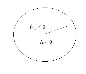
Figure 1: Circularly symmetric space–time filled with both $\theta_{\mu\nu}$ and cosmological constant $\Lambda$. Note that the case $\theta_{\mu\nu}=0$ yields BTZ black hole.

IV.1 Isotropic solutions

Considering an isotropic pressure for the source $\theta_{\mu\nu}$ ovalle2018a implies

$$\theta^{1}_{1}=\theta^{2}_{2}.$$ (27)

Combining Eqs. (18) and (19) leads to

$$f^{\prime}+\frac{2rf}{L^{2}M-r^{2}}=0,$$ (28)

from where

$$f=c_{1}L^{2}\left(-M+\frac{r^{2}}{L^{2}}\right),$$ (29)

whith $c_{1}$ a constant of integration with dimension of inverse of length squared. From Eq. (12) we obtain

$$e^{-\lambda}=\left(1+\alpha c_{1}L^{2}\right)\left(-M+\frac{r^{2}}{L^{2}}\right).$$ (30)

Replacing in Eqs. (4), (5), (6) and (7) we obtain the line element

$$ds^{2}=(-M+\frac{r^{2}}{L^{2}})dt^{2}-\frac{dr^{2}}{(\alpha c_{1}L^{2}+1)\left(-M+\frac{r^{2}}{L^{2}}\right)}-r^{2}d\phi,$$ (31)

and the matter content

$$\tilde{\rho} = -\frac{1+\alpha c_{1}L^{2}}{8\pi L^{2}}$$

$$\tilde{p}_{r}=\tilde{p}_{\perp} = \frac{1+\alpha c_{1}L^{2}}{8\pi L^{2}}.$$ (32)

It is worth mentioning that Eqs. (31) and (IV.1) correspond to an isotropic solution for $2+1$ dimension. In fact, a straightforward calculation reveals that the curvature scalars read

$$R = 6\left(\alpha c_{1}+\frac{1}{L^{2}}\right)$$

$$Ricc^{2} = \frac{12\left(\alpha c_{1}L^{2}+1\right)^{2}}{L^{4}}$$

$$\mathcal{K} = \frac{12\left(\alpha c_{1}L^{2}+1\right)^{2}}{L^{4}},$$ (33)

where $R$, $Ricc^{2}$ and $\mathcal{K}$ stand form he Ricci, Ricci squared and the Kretschmann scalars respectively. Note that from Eqs. (IV.1) we recover BTZ only if $\alpha\to 0$.

IV.2 Conformally symmetric solutions

In this case we impose

$$\theta^{2}_{2}=-\theta^{0}_{0}-\theta^{1}_{1},$$ (34)

which implies that the source is traceless as required by the conformal symmetry. Combining condition (34) with (17), (18) and (19) we obtain

$$\frac{f^{\prime}\left(L^{2}M-2r^{2}\right)}{r}+\frac{2f\left(r^{2}-2L^{2}M\right)}{L^{2}M-r^{2}}=0,$$ (35)

from where

$$f=c_{1}\frac{\left(r^{2}-L^{2}M\right)}{\left(2r^{2}-L^{2}M\right)^{3/2}}.$$ (36)

In this case $c_{1}$ is a constant of integration with dimension of length. In order to obtain the line element and the matter content of the new solution we perform the same procedure followed in the last section. In this case combining (36) and (12) with (4), (5), (6) and (7), we obtain the $g^{rr}$ component of the metric

$$e^{-\lambda}=\frac{\left(\frac{r^{2}}{L^{2}}-M\right)\left(\alpha c_{1}L^{2}+\left(2r^{2}-L^{2}M\right)^{3/2}\right)}{\left(2r^{2}-L^{2}M\right)^{3/2}},$$ (37)

and the anisotropic matter content given by

$$\tilde{\rho} = \frac{L^{2}r^{2}}{8\pi\left(L^{3}M-2Lr^{2}\right)^{2}}\left(\frac{\alpha c_{1}}{\sqrt{2r^{2}-L^{2}M}}4M\right)$$ (38)

$$-\frac{L^{4}M}{8\pi\left(L^{3}M-2Lr^{2}\right)^{2}}\left(\frac{2\alpha c_{1}}{\sqrt{2r^{2}-L^{2}M}}+M\right)$$

$$-\frac{4r^{4}}{8\pi\left(L^{3}M-2Lr^{2}\right)^{2}}$$

$$\tilde{p}_{r} = \frac{1}{8\pi}\left(\frac{\alpha c_{1}}{\left(2r^{2}-L^{2}M\right)^{3/2}}+\frac{1}{L^{2}}\right)$$ (39)

$$\tilde{p}_{\perp} = -\frac{L^{2}r^{2}}{8\pi\left(L^{3}M-2Lr^{2}\right)^{2}}\left(\frac{\alpha c_{1}}{\sqrt{2r^{2}-L^{2}M}}+4M\right)$$ (40)

$$+\frac{L^{4}M}{8\pi\left(L^{3}M-2Lr^{2}\right)^{2}}\left(M-\frac{\alpha c_{1}}{\sqrt{2r^{2}-L^{2}M}}\right)$$

$$+\frac{4r^{4}}{8\pi\left(L^{3}M-2Lr^{2}\right)^{2}}.$$

Note that in this case the method leads to an anisotropic solutions with curvature scalars given by

$$R = \frac{6}{L^{2}}$$ (41)

$$Ricc^{2} = \frac{12}{L^{4}}-\frac{6\alpha^{2}c_{1}^{2}\left(L^{4}M^{2}-L^{2}Mr^{2}+r^{4}\right)}{\left(L^{2}M-2r^{2}\right)^{5}}$$ (42)

$$\mathcal{K} = \frac{12}{L^{4}}-\frac{24\alpha^{2}c_{1}^{2}\left(L^{4}M^{2}-L^{2}Mr^{2}+r^{4}\right)}{\left(L^{2}M-2r^{2}\right)^{5}}.$$ (43)

As in the previous case the BTZ solution is recovered in the limit $\alpha\to 0$.

Now let us explore the causal structure of the solution. First note that the solution still have a Killing horizon ($e^{\nu}=0$) at $r_{H}=L\sqrt{M}$. Even more, $e^{-\lambda}$ diverges for the critical radius

$$r_{c}=L\sqrt{\frac{M}{2}}<r_{H}.$$ (44)

In fact, this critical radius must be considered a real singularity provided some of the curvature scalar diverge at the same point. For this geometry we have two causal horizons at $e^{-\lambda}=0$. The first one is at $r_{H}$, as in the BTZ case, but there is a second root given by

$$r_{0}=\frac{\sqrt{\alpha^{2/3}c_{1}^{2/3}L^{4/3}+L^{2}M}}{\sqrt{2}}.$$ (45)

It is worth noticing that $r_{0}\geq r_{c}$ and depending on the values of the constant will be inside or outside the Killing horizon $r_{H}$. In particular for

$$\alpha c_{1}<LM^{2/3},$$ (46)

we obtain that $r_{0}$ is in the interval $r_{c}<r_{0}<r_{H}$ and $r_{0}>r_{H}$ for $\alpha c_{1}>LM^{2/3}$. In order to avoid unacceptable space–time signature outside $r_{H}$ we should demand the condition given by Eq. (46). In this case the behaviour resembles that of a charged BH solution but with singularity at certain critical radius, $r_{c}$, instead of at the origin.

IV.3 Linear anisotropic source

In this case, we choose a linear anisotropic source with equation of state give by

$$\theta^{0}_{0}=a\theta^{1}_{1}+b\theta^{2}_{2}.$$ (47)

Combination of (47) with (17), (18) and (19) leads to

$$\frac{2f\left(L^{2}M(a+b)-ar^{2}\right)}{L^{2}M-r^{2}}+\frac{f^{\prime}\left((b-1)r^{2}+L^{2}M\right)}{r}.$$ (48)

from where

$$f=c_{1}\left(r^{2}-L^{2}M\right)\left((b-1)r^{2}+L^{2}M\right)^{-\frac{a}{b-1}-1}.$$ (49)

The constant of integration has dimensions of$\textnormal{(Lenght)}^{-(2+\frac{2a}{1-b}-2)}$. Combining (49) and (12) we obtain

$$e^{-\lambda}=F_{0}+\alpha c_{1}L^{4}\left(\frac{r^{2}}{L^{2}}-M\right)\left(\frac{(b-1)r^{2}}{L^{2}}+M\right)^{\Gamma}.$$ (50)

where

$$F_{0}=\frac{r^{2}}{L^{2}}-M,$$ (51)

and $\Gamma=-\frac{a}{b-1}-1$. To complete the analysis, we compute the content of the isotropic matter responsible of this geometry by replacing (49) and (12) in (5), (6) and (7) to obtain

$$\tilde{\rho} = -\frac{1}{8\pi L^{2}}-\frac{\alpha c_{1}\left(L^{2}M(a+b)-ar^{2}\right)}{8\pi}\times$$ (52)

$$\times\frac{\left((b-1)r^{2}+L^{2}M\right)^{\Theta}}{8\pi}$$

$$\tilde{p}_{r} = \frac{\alpha c_{1}L^{2}\left(\frac{r^{2}}{L^{2}}-M\right)\left((b-1)r^{2}+L^{2}M\right)^{\Gamma}}{8\pi L^{2}}$$ (53)

$$+\frac{\left(\frac{r^{2}}{L^{2}}-M\right)}{8\pi L^{2}}$$

$$\tilde{p}_{\perp} = -\frac{\alpha c_{1}L^{2}F(z)\left((b-1)r^{2}+L^{2}M\right)^{\Theta}}{8\pi L^{6}}$$ (54)

$$+\frac{L^{4}M+L^{2}Mr^{2}-2L^{2}r^{2}-r^{4}}{8\pi L^{6}},$$

where $\Theta=-\frac{a}{b-1}-2$ and

$$F(z) = L^{2}r^{4}(a+(b-2)M-b+1)-(b-1)r^{6}$$ (55)

$$+L^{6}M^{2}+L^{4}Mr^{2}(-a+M-2).$$

Now we analyse the causal structure directly from equations (52) . First, note that we can avoid the apparition of any singularity taking $\Theta>0$ which implies $b<1$ and $a>2(1-b)$. Second, observe that $e^{-\lambda}$ has two roots: one corresponding to the Killing horizon $r_{H}=L\sqrt{M}$ and the other at

$$r_{0}=\frac{\sqrt{\left(-\frac{1}{\alpha c_{1}L^{2}}\right){}^{\frac{a}{a+b-1}-1}-L^{2}M}}{\sqrt{b-1}}.$$ (56)

In this case, $r_{0}$ could be avoided for suitable choices of the parameters $\alpha$, $c_{1}$, $a$ and $b$. In particular, note that no real solutions can be obtained for $r_{0}$ when

$$\left(-\frac{1}{\alpha c_{1}L^{2}}\right){}^{\Gamma}<L^{2}M.$$ (57)

V Conclusions

In this work we implemented the Minimal Geometric Deformation–decoupling method in $2+1$ circularly symmetric and static space–times obtaining that both the isotropic and the anisotropic sector fulfil Einstein field equations in contrast to the cases studied in $3+1$ dimensions, where the anisotropic sector satisfies certain “quasi–Einstein” field equations. In this sense the Einstein Field Equations for a collection of sources can be transformed into a collection of Einstein’s equations, one for each source. As an example, we implemented the decoupling method to obtain new solutions from the well known static BTZ geometry. In particular, the anisotropic system were solved providing suitable equations of state for the source $\theta_{\mu\nu}$ namely the isotropic, the conformal and the linear equation of state. The results are in concordance with their $3+1$ counterparts obtained in reference ovalle2018a in the sense that some extra structures such as causal horizons and singularities appear as a consequence of the Minimal Geometry Deformation-decoupling. In adition, it was shown that in the case of linear equation of state those extra structures can be avoided for certain values of the free parameters of the solution, as shown in reference ovalle2018 for 3+1 spacetimes.
We conclude this paper by noting that the method here developed can be easily applied to obtain new and relevant solutions taking as the isotropic sector any of the already known 2+1 space–times.

References

- (1) J. Ovalle. Mod. Phys. Lett. A 23, 3247 (2008).
- (2) L. Randal, R. Sundrum. Phys. Rev. Lett. 83, 3370 (1999).
- (3) L. Randal, R. Sundrum. Phys. Rev. Lett. 83, 4690 (1999).
- (4) J. Ovalle. Int. J. Mod. Phys. D 18, 837 (2009).
- (5) J. Ovalle. Mod. Phys. Lett. A 25, 3323 (2010).
- (6) R. Casadio, J. Ovalle. Phys. Lett. B 715, 251 (2012).
- (7) J. Ovalle, F. Linares. Phys. Rev. D 88, 104026 (2013).
- (8) J. Ovalle, F. Linares, A. Pasqua, A. Sotomayor. Class. Quantum Grav. 30,175019 (2013).
- (9) R. Casadio, J. Ovalle, R. da Rocha. Class. Quantum Grav. 30, 175019 (2014).
- (10) R. Casadio, J. Ovalle. Class. Quantum Grav. 32, 215020 (2015).
- (11) J. Ovalle. Int. J. Mod. Phys. Conf. Ser. 41, 1660132 (2016).
- (12) J. Ovalle, L.A. Gergely, R. Casadio, Class. Quantum Grav., 32, 045015 (2015).
- (13) R. Casadio, J. Ovalle, R. da Rocha, EPL, 110, 40003 (2015).
- (14) R. T. Cavalcanti, A. Goncalves da Silva, R. da Rocha, Class. Quantum Grav. 33, 215007(2016).
- (15) R. Casadio, R. da Rocha, Phys. Lett. B 763, 434 (2016).
- (16) J. Ovalle. Phys. Rev. D 95, 104019 (2017).
- (17) R. da Rocha, Phys. Rev. D 95, 124017 (2017).
- (18) R. da Rocha, Eur. Phys. J. C 77, 355 (2017).
- (19) R. Casadio, P. Nicolini, R. da Rocha. arXiv:1709.09704 [hep-th].
- (20) J. Ovalle, R. Casadio, R. da Rocha, A. Sotomayor. Eur. Phys. J. C 78, 122 (2018).
- (21) M.Estrada, F. Tello-Ortiz. arXiv:1803.02344v3 [gr-qc].
- (22) J. Ovalle, R. Casadio, R. da Rocha, A. Sotomayor, Z. Stuchlik. arXiv:1804.03468 [gr-qc].
- (23) C. Las Heras, P. Leon. arXiv:1804.06874v3 [gr-qc].
- (24) L. Gabbanelli, A. Rincón, C. Rubio, arXiv:1802.08000 [gr-qc].
- (25) M. Sharif, Sobia Sadiq. arXiv:1804.09616v1 [gr-qc].
- (26) A. Fernandes-Silva, A. J. Ferreira-Martins, R. da Rocha; arXiv:1803.03336 [hep-th].
- (27) A. Fernandes-Silva, R. da Rocha, Eur. Phys.J. C 78 (2018) 271.
- (28) A. Staruszkiewicz Acta Phys. Polon. 24, 735 (1963).
- (29) A. A. García–Díaz, Exact Solutions in Three–Dimensional Gravity, Cambridge University Press (2017).
- (30) M. Bañados, C. Teitelboim, J. Zanelli, Phys. Rev. Lett. 69, 1849 (1992).