Dispersion Theory in Electromagnetic Interactions

Abstract

We review various applications of dispersion relations (DRs) to the electromagnetic structure of hadrons. We discuss the way DRs allow one to extract information on hadron structure constants by connecting information from complementary scattering processes. We consider the real and virtual Compton scattering processes off the proton, and summarize recent advances in the DR analysis of experimental data to extract the proton polarizabilities, in comparison with alternative studies based on chiral effective field theories. We discuss a multipole analysis of real Compton scattering data, along with a DR fit of the energy-dependent dynamical polarizabilities. Furthermore, we review new sum rules for the double-virtual Compton scattering process off the proton, which allow for model independent relations between polarizabilities in real and virtual Compton scattering, and moments of nucleon structure functions. The information on the double-virtual Compton scattering is used to predict and constrain the polarizability corrections to muonic hydrogen spectroscopy.

1 Introduction

The starting point of dispersion relations (DRs) dates back to 1926-1927 with the historic papers of Kronig [1] and Kramers [2], discussing the classical dispersion of light and the relation between the real and imaginary parts of the index of refraction. They emphasized that a specific relation between the real (dispersive) and imaginary (absorptive) part of the index of refraction was based on the fundamental requirement of causality, in addition to the usual conditions on the scattering matrix, namely, unitarity and Lorentz invariance. The quantum mechanical formulation of the causality condition was then used in the work by Gell-Mann, Goldberger and Thirring [3] to derive DRs for forward Compton scattering, using perturbation theory for the electromagnetic interaction. Soon after, Goldberger [4] posed the proof on more general grounds, going beyond the limitation of perturbation theory. These pioneering works laid the foundations for the derivation of a number of sum rules, obtained by combining DRs and low energy theorems [5, 6, 7, 8] for the forward real Compton scattering (RCS) amplitude. The best known sum rules are the Baldin sum rule [9] for the sum of the dipole polarizabilities and the Gerasimov-Drell-Hearn (GDH) sum rule [10, 11] for the anomalous magnetic moment. Further relations can be obtained considering higher-order terms in the low-energy expansion (LEX) of the RCS forward amplitudes. These sum rules all relate a measured electromagnetic structure quantity to an integral over a photo-absorption cross section on the nucleon, and are thus model-independent relations. The photo-absorption cross sections are by now fairly well known, and have been used in various phenomenological works for the evaluation of the forward RCS sum rules, as reviewed in Section 2.1.

Along with the study of DRs for forward RCS, in the 1960s there was considerable work to extend the general formalism of DRs to non-forward RCS, see, for example, Refs. [12, 13, 14]. However, DRs for non-forward RCS have become a practicable tool for a detailed investigation of nucleon structure only recently thanks to the advent of high-precision experiments with electromagnetic probes. Among the most successful applications is the analysis of RCS observables from low energies up to the $\Delta(1232)$-resonance region to extract information on the nucleon static polarizabilities [15, 16, 17, 18, 19, 20]. The static polarizabilities are nucleon structure constants which measure the global strength of the induced current and magnetization densities in the nucleon under the influence of an external quasi-static electromagnetic field. Polarizabilities acquire an energy dependence due to internal relaxation mechanisms, resonances and particle production thresholds in a physical system. This energy dependence defines the dynamical polarizabilities [16], which parametrize the response of the internal degrees of freedom of a composite object to an external, real photon field of arbitrary energy. Recent advances in the extraction of both the static and dynamical polarizabilities within different variants of DR techniques are summarized in Sections 2.2 and 2.3.

When considering the virtual Compton scattering (VCS) process, where the incident real photon is replaced by a virtual photon, we can get access to generalized polarizabilities (GPs) [21, 22]. They depend on the virtuality of the incident photon and allow us to map out the spatial distribution of the polarization densities in a target. The DR formalism for VCS on a proton has been developed more recently [23, 24], and applied to a new generation of VCS experiments to extract the scalar GPs of the proton. The state-of-the-art of the dispersion analysis for VCS is presented in Section 3.

The most general case of a double-virtual Compton process, with both initial and final virtual photons, has up to now only been studied in some special limits. The most useful extension is given by the forward double-virtual Compton (VVCS) process, where the initial and final photons have the same non-zero spacelike virtuality. In contrast to the processes discussed above, the forward VVCS process is not directly measurable. However, DRs provide a powerful tool to reconstruct the VVCS amplitudes from the empirical information on the electro-absorption cross sections [25, 26], encoded in the nucleon structure functions This is possible provided the integrals converge, otherwise a subtraction is required. One can thus formulate extensions of the Baldin, GDH, and other sum rules, through moments of nucleon structure functions [27, 28, 29, 18]. Such relations can be tested provided one can rely on a theory, such as chiral effective field theory, to calculate the coefficients in the LEXs of the VVCS amplitudes. Recently, several new sum rules have been developed which yield model-independent relations between polarizabilities in RCS, VCS, and moments of nucleon structure functions. We review the status of the field of VVCS in Section 4. In Section 5, we then discuss how the VVCS amplitudes enter to predict and constrain the polarizability corrections to muonic hydrogen spectroscopy.

We conclude this review in Section 6 and outline some remaining issues for future work.

2 Real Compton scattering

In this section, we introduce the sum rules for forward RCS along with a review of the most recent evaluations of the corresponding dispersion integrals. We then discuss the general formalism of DRs for non-forward Compton scattering and its application to the extraction of the static and dynamical polarizabilities.

2.1 Forward dispersion relations

Let us consider the kinematics of the RCS reaction, i.e.

$$\gamma(q)+N(p)\rightarrow\gamma(q^{\prime})+N(p^{\prime}),$$ (1)

where the variables in brackets denote the four-momenta of the participating particles. The initial and final photons are characterized by the polarization four-vectors $\epsilon_{\lambda}=(0,\boldsymbol{\epsilon}_{\lambda})$ and $\epsilon^{\prime}_{\lambda^{\prime}}=(0,\boldsymbol{\epsilon}_{\lambda^{\prime}})$, respectively. The familiar Mandelstam variables are

$$s=(p+q)^{2},\quad u=(q-p^{\prime})^{2},\quad t=(q-q^{\prime})^{2},$$ (2)

which are constrained by $s+t+u=2M^{2}$, with $M$ the nucleon mass. To describe Compton scattering, we can choose the two Lorentz invariant variables $t$ and $\nu$, with the the crossing symmetric variable $\nu$ defined by $\nu=(s-u)/4M.$ They are related to the initial ($E_{\gamma}$) and final ($E^{\prime}_{\gamma}$) photon lab energy and to the scattering angle $\theta_{{\rm lab}}$ by

$$\nu=E_{\gamma}+\frac{t}{4M}=\frac{1}{2}(E_{\gamma}+E^{\prime}_{\gamma}),\qquad t=-4E_{\gamma}\,E^{\prime}_{\gamma}\,\sin^{2}(\theta_{\rm lab}/2)=-2M(E_{\gamma}-E^{\prime}_{\gamma}).$$

In the forward direction, $\nu=E_{\gamma}=E^{\prime}_{\gamma}$ coincides with the initial and final photon energy and $t=0$. In this case, the most general form for the Compton amplitude can be constructed from the independent vectors at our disposal, i.e. $\boldsymbol{\epsilon}$, $\boldsymbol{\epsilon}^{\prime}$, $\boldsymbol{q}=\boldsymbol{q}^{\prime}$, and the proton spin operator $\boldsymbol{\sigma}$, by requiring to be linear in $\boldsymbol{\epsilon}$ and $\boldsymbol{\epsilon}^{\prime}$, with the transverse gauge condition $\boldsymbol{\epsilon}\cdot\boldsymbol{q}=\boldsymbol{\epsilon}^{\prime}\cdot\boldsymbol{q}^{\prime}=0$, and invariant under rotation and parity transformations. This leads to

$$T(\nu,t=0)={\boldsymbol{\epsilon}}^{\prime*}_{\lambda^{\prime}}\cdot\boldsymbol{\epsilon}_{\lambda}f(\nu)+i\boldsymbol{\sigma}\cdot(\boldsymbol{\epsilon}^{\prime}_{\lambda^{\prime}}{}^{*}\times\boldsymbol{\epsilon}_{\lambda})g(\nu).$$ (3)

Because of crossing symmetry, the amplitude $T$ also has to be invariant under the transformation $\boldsymbol{\epsilon}\leftrightarrow\boldsymbol{\epsilon}^{\prime}$ and $\nu\leftrightarrow-\nu$, with the result that $f$ and $g$ are, respectively, an even and odd function of $\nu$, i.e. $f(-\nu)=f(\nu)$ and $g(-\nu)=-g(\nu)$. Depending on the relative orientation of the spins, the absorption of the photon leads to hadronic excited states with spin projections $1/2$ and $3/2$. The optical theorem expresses the unitarity of the scattering matrix by relating the respective cross sections, $\sigma_{1/2}$ and $\sigma_{3/2},$ to the imaginary parts of the forward scattering amplitudes

$${\rm Im}\,f(\nu) = \frac{\nu}{8\pi}\left(\sigma_{1/2}(\nu)+\sigma_{3/2}(\nu)\right)\equiv\frac{\nu}{4\pi}\sigma_{T}(\nu),$$

$${\rm Im}\,g(\nu) = \frac{\nu}{8\pi}\left(\sigma_{1/2}(\nu)-\sigma_{3/2}(\nu)\right)\equiv\frac{\nu}{4\pi}\sigma_{TT}(\nu),$$ (4)

where $\sigma_{T}$ and $\sigma_{TT}$ correspond to the total photo-absorption cross section and to the transverse-transverse interference term, respectively. Due to the smallness of the fine structure constant, we may neglect all purely electromagnetic processes, and shall consider only photo-absorption due to the hadronic channels starting at pion production threshold, $\nu_{thr}=m_{\pi}+m_{\pi}^{2}/2M\simeq 150$ MeV, where $m_{\pi}$ is the pion mass. In order to set up the dispersion integrals, we have to study the behavior of the absorption cross sections for large energies. The total cross section $\sigma_{T}$ is essentially constant above the resonance region, with a slow logarithmic increase at the highest energies, and therefore we must subtract the DR for $f$. If we subtract at $\nu=0$, we also remove the nucleon-pole terms at this point. Using causality, crossing symmetry, and the optical theorem 4, the subtracted DR reads:

$$\mathrm{Re}\,f(\nu) = f(0)+\frac{\nu^{2}}{2\pi^{2}}{\cal P}\int_{\nu_{thr}}^{+\infty}{\rm d}\nu^{\prime}\frac{\sigma_{T}(\nu^{\prime})}{\nu^{\prime 2}-\nu^{2}}.$$ (5)

For the odd function, we can instead assume the following unsubtracted DR:

$$\mathrm{Re}\,g(\nu) = \frac{\nu}{2\pi^{2}}{\cal P}\int_{\nu_{thr}}^{+\infty}{\rm d}\nu^{\prime}\frac{\nu^{\prime}\sigma_{TT}(\nu^{\prime})}{\nu^{\prime 2}-\nu^{2}}.$$ (6)

The behaviour of the scattering amplitudes at low energies is predicted by low-energy theorems (LETs) [5, 6, 7, 8] in the following form:

$$f(\nu) = -\frac{e^{2}e^{2}_{N}}{4\pi M}+(\alpha_{E1}+\beta_{M1})\nu^{2}+[\alpha_{E1\nu}+\beta_{M1\nu}+\frac{1}{12}(\alpha_{E2}+\beta_{M2})]\nu^{4}+{\cal O}(\nu^{6}),$$ (7)

$$g(\nu) = -\frac{e^{2}\kappa_{N}^{2}}{8\pi M^{2}}\nu+\gamma_{0}\nu^{3}+\bar{\gamma}_{0}\nu^{5}+{\cal O}(\nu^{7}).$$ (8)

The leading terms in the expansion of Eqs. 7 and 8 are due to the intermediate nucleon states (Born terms), and depend solely on the static properties of the nucleon, i.e. the charge $ee_{N}$, with $e_{p}=1$ and $e_{n}=0$, the mass $M$, and the anomalous magnetic moment $(e/2M)\kappa_{N}$, with $\kappa_{p}=1.79$ and $\kappa_{n}=-1.91$. Only the higher-order terms contain information on the internal structure (spectrum and excitation strengths) of the complex system. In the case of the spin-independent amplitude $f(\nu)$, the term ${\cal O}(\nu^{2})$ describes Rayleigh scattering and yields information on the internal nucleon structure through the electric ($\alpha_{E1}$) and magnetic ($\beta_{M1}$) dipole polarizabilities, while the higher-order terms at ${\cal O}(\nu^{4})$ contain contributions of dipole retardation ($\alpha_{E1\nu}$ and $\beta_{M1\nu}$) and higher multipoles ($\alpha_{E2}$ and $\beta_{M2}$). In the case of the spin-flip amplitude $g(\nu)$, the leading term is determined by the anomalous magnetic moment, and the higher-order terms contain information on the spin structure through the forward spin polarizability (FSP) $\gamma_{0}$ and higher-order FSP $\bar{\gamma}_{0}$. These results can be compared with the coefficients of the Taylor series expansion around $\nu=0$ of the integrals in Eqs. 5 and 6. In the spin-independent sector, this yields the Baldin sum rule [9]:

$$\alpha_{E1}+\beta_{M1}=\frac{1}{2\pi^{2}}\int_{\nu_{thr}}^{+\infty}{\rm d}\nu^{\prime}\frac{\sigma_{T}(\nu^{\prime})}{\nu^{\prime 2}},$$ (9)

and a fourth-order Baldin sum rule for the higher-order static polarizabilities [30]:

$$\alpha_{E1\nu}+\beta_{M1\nu}+\frac{1}{12}(\alpha_{E2}+\beta_{M2})=\frac{1}{2\pi^{2}}\int_{\nu_{thr}}^{+\infty}{\rm d}\nu^{\prime}\frac{\sigma_{T}(\nu^{\prime})}{\nu^{\prime 4}}.$$ (10)

In the spin dependent sector, the leading term yields the Gerasimov-Drell-Hearn (GDH) sum rule [10, 11]:

$$\frac{\pi e^{2}\kappa^{2}_{N}}{4M^{2}}=-\int_{\nu_{thr}}^{+\infty}{\rm d}\nu^{\prime}\frac{\sigma_{TT}(\nu^{\prime})}{\nu^{\prime}},$$ (11)

while the higher-order coefficients gives the Gell-Mann, Goldberger, and Thirring (GGT) sum rule [5, 3] for the FSP $\gamma_{0}$ and a sum rule for the higher-order FSP $\bar{\gamma}_{0}$ [31]:

$$\gamma_{0}=\frac{1}{2\pi^{2}}\int_{\nu_{thr}}^{+\infty}{\rm d}\nu^{\prime}\frac{\sigma_{TT}(\nu^{\prime})}{\nu^{\prime 3}},\qquad\bar{\gamma}_{0}=\frac{1}{2\pi^{2}}\int_{\nu_{thr}}^{+\infty}{\rm d}\nu^{\prime}\frac{\sigma_{TT}(\nu^{\prime})}{\nu^{\prime 5}}.$$ (12)

These dispersive integrals have been evaluated from the available experimental data on the total photo-absorption cross section and helicity-difference photo-absorption cross section, using different prescriptions for the extrapolation in the kinematical regions not covered by the data. The results from the most recent evaluations are collected in Table 1.

Table 1: Empirical evaluations of the Baldin sum rule (Eq. 9), the fourth-order relation in the spin-independent sector (Eq. 10), the GDH sum rule (Eq. 11), and the leading- and higher-order FSPs (Eq. 12).

	Baldin	IV order	GDH	$\gamma_{0}$	$\bar{\gamma}_{0}$
	($10^{-4}$ fm3)	($10^{-4}$ fm5)	$(\mu$b)	($10^{-6}$ fm4)	($10^{-6}$ fm6)
Babusci et al. [32]	$13.69\pm 0.14$
A2 [33]	$13.8\pm 0.4$
Gryniuk et al. [30]	$14.0\pm 0.2$	$6.04\pm 0.4$
GDH & A2 [34, 35, 36]			$212\pm 17.1$	$-101\pm 13$
Pasquini et al. [31]			$210\pm 15.2$	$-90\pm 14$	$60\pm 10$
Gryniuk et al. [37]			$204.5\pm 21.4$	$-92.9\pm 10.5$	$48.4\pm 8.2$
sum rule			204.78

The database for the total photo-absorption cross section covers the energy intervals [0.2, 4.2] GeV [38, 39, 40] and [18, 185] GeV [41], with additional two measurements at 200 GeV [42] and 209 GeV [43]. The contribution to the sum rules from $\nu_{thr}$ to 0.2 GeV was determined on the basis of various multipole analyses for pion photo-production, i.e. MAID [44, 45], SAID [46] and HDT [47], while the contribution from the region above 2 GeV, extrapolated to $+\infty$, was obtained from different fits, mainly based on Regge theory.

The evaluations of the sum rules in the spin-dependent sector are mainly based on the recent GDH-Collaboration data for the helicity-difference photo-absorption cross section, covering the region from 0.2 to 2.9 GeV [48, 34, 35]. In Ref. [31], the data set has been supplemented with measurements of the polarized differential cross sections for the $n\pi^{+}$ channel up to energy equal to $0.175$ GeV. These data points have been extrapolated into the unmeasured angular range with the HDT analysis, in order to reconstruct the helicity-difference total cross section. Considering the energy-weighting factors in the dispersion integrals of Eqs. 11 and 12, one finds that the most crucial contribution for the FSP and higher-order FSP is from the threshold region up to the first resonance region. In particular, the contribution from the charged-pion channel is characterized by a strong competition between the $E_{0+}$ multipole above threshold and the $M_{1+}$ near the $\Delta(1232)$ resonance, whereas the neutral-pion channel is almost completely described by the $\Delta(1232)$ resonance effects. As a result, the evaluation of the sum rules for the FSPs can be particularly sensitive to the multipole analysis used for the extrapolation of the integrand into the unmeasured region near threshold. The final results, as summarized in Table 1, are all consistent, within the error bars, and reproduce the GDH sum rule value (lhs of Eq. 11).

2.2 Static polarizabilities

The physical content of the static polarizabilities can be best illustrated using effective multipole interactions for the coupling of the electric ($\boldsymbol{E}$) and magnetic ($\boldsymbol{H}$) fields of a source with the internal structure of the nucleon. When expanding the Compton scattering amplitude in the photon energy, the second- and fourth-order contributions read [16, 49]:

$$H_{\rm{eff}}^{(2)} = -4\pi\left[{\textstyle\frac{1}{2}}\,\alpha_{E1}\,\boldsymbol{E}\,^{2}+{\textstyle\frac{1}{2}}\,\beta_{M1}\,\boldsymbol{H}\,^{2}\right],$$ (13)

$$H_{\rm{eff}}^{(4)} = -4\pi\left[{\textstyle\frac{1}{2}}\,\alpha_{E1\nu}\,\dot{\boldsymbol{E}}\,^{2}+{\textstyle\frac{1}{2}}\,\beta_{M1\nu}\,\dot{\boldsymbol{H}}\,^{2}+{\textstyle\frac{1}{12}}\,\alpha_{E2}\,E_{ij}^{2}+{\textstyle\frac{1}{12}}\,\beta_{M2}\,H_{ij}^{2}\right],$$ (14)

where the dots denote a time derivative, and the quadrupole field tensors are denoted by:

$$E_{ij}=\frac{1}{2}\left(\nabla_{i}E_{j}+\nabla_{i}E_{i}\right),\qquad H_{ij}=\frac{1}{2}\left(\nabla_{i}H_{j}+\nabla_{i}H_{i}\right).$$ (15)

In Eq. 13 we recognize the static electric ($\alpha_{E1}$) and magnetic ($\beta_{M1}$) polarizabilities, describing the dipole deformations of the electric and magnetic densities inside the nucleon induced by external static electromagnetic fields. At higher order, the terms in $\alpha_{E1\nu}$ and $\beta_{M1\nu}$ are retardation or dispersive corrections to the lowest-order static polarizabilities and describe the response of the system to time-dependent fields. The parameters $\alpha_{E2}$ and $\beta_{M2}$ represent quadrupole polarizabilities and measure the electric and magnetic quadrupole moments induced in a system in the presence of an applied field gradient. The dependence on the spin enters at third-order via the following effective Hamiltonian

$${H}_{\rm{eff}}^{(3)} = -4\pi\left[{\textstyle\frac{1}{2}}\gamma_{E1E1}\,\boldsymbol{\sigma}\cdot(\boldsymbol{E}\times\dot{\boldsymbol{E}})+{\textstyle\frac{1}{2}}\gamma_{M1M1}\,\boldsymbol{\sigma}\cdot(\boldsymbol{H}\times\dot{\boldsymbol{H}})\right.$$ (16)

$$\left.-\gamma_{M1E2}\,E_{ij}\,\sigma_{i}H_{j}+\gamma_{E1M2}\,H_{ij}\,\sigma_{i}E_{j}\right],$$

where the four spin polarizabilities $\gamma_{E1E1}$, $\gamma_{M1M1}$, $\gamma_{M1E2}$, and $\gamma_{E1M2}$ are related to a multipole expansion [16], as reflected in the subscript notation. The FSP $\gamma_{0}$, and the so-called backward spin polarizability $\gamma_{\pi}$, entering the Compton scattering amplitudes at backward angles, are then obtained through the following combinations:

$$\gamma_{0}=-\gamma_{E1E1}-\gamma_{M1M1}-\gamma_{E1M2}-\gamma_{M1E2},\quad\gamma_{\pi}=-\gamma_{E1E1}+\gamma_{M1M1}-\gamma_{E1M2}+\gamma_{M1E2}.\quad$$ (17)

The extraction of the polarizabilities from RCS data has become a mature field in recent years. It is performed mainly by three techniques. The first one is a low-energy expansion (LEX) of the RCS cross sections. Unfortunately this procedure is only applicable at photon energies well below 100 MeV, which makes a precise extraction a rather challenging task because of the very low sensitivity to the polarizabilities at these energies. This sensitivity is increased by measuring RCS observables around pion threshold and into the $\Delta(1232)$ region. A second formalism which has been successfully applied to RCS data up to these energies makes use of DRs. It has been worked out for both unsubtracted [15] and subtracted [17, 20] DRs. Recently, a third approach has been developed within the framework of a chiral effective field theory [50, 51, 52, 53, 54, 55, 56], for energies up to the $\Delta$-resonance region.

In order to set up the DR framework, the first step is to construct a complete set of amplitudes in accordance with relativity and free of kinematical singularities. According to L’vov et al. [15], they can be identified as six Lorentz invariant amplitudes $A_{i}(\nu,t)$, $i=1,\dots,6$, which depend on the invariants $\nu$ and $t$, and obey the crossing symmetry relation $A_{i}(\nu,t)=A_{i}(-\nu,t)$. Next, causality requires certain analytic properties of the amplitudes, which allow for a continuation of the scattering amplitudes into the complex plane and lead to DRs connecting the real and imaginary parts of these amplitudes. The imaginary parts can be replaced by photo-production amplitudes using unitarity, and as a result we can complete the Compton amplitudes from experimental information on photo-absorption reactions. In particular, the unsubtracted DRs at fixed $t$ reads:

$${\rm Re}A_{i}(\nu,t)=A_{i}^{B}(\nu,t)+{2\over\pi}{\mathcal{P}}\int_{\nu_{thr}}^{+\infty}d\nu^{\prime}{{\nu^{\prime}\mathrm{Im}_{s}A_{i}(\nu^{\prime},t)}\over{\nu^{\prime 2}-\nu^{2}}},$$ (18)

where $A_{i}^{B}$ are the nucleon pole contributions and ${\mathcal{P}}$ denotes the principal value integral, which runs from the pion production threshold upwards. Taking into account the energy weighting, the threshold pion production and the decay of low-lying resonances yield the largest contributions to the integral. With existing information on these processes and reasonable assumptions on the lesser known higher part of the spectrum, the integrand can be constructed up to centre-of-mass (cm) energies $W\simeq 2$ GeV. However, a Regge analysis for the asymptotic behavior does not guarantee the convergence of the integrals for the amplitudes $A_{1}$ and $A_{2}$. This behavior is mainly due to fixed poles in the $t$ channel, notably the exchange of a neutral pion for $A_{2}$ and of a $\sigma$ meson for $A_{1}$. To circumvent this problem, L’vov et al. [15] proposed to use finite-energy sum rules for these two amplitudes, i.e. to close the contour integral in the complex plane by a semicircle of finite radius $\nu_{max}$ and to identify the contribution from the semicircle with the asymptotic contribution described by $t$-channel poles. This procedure is relatively safe for $A_{2}$ because the $\pi^{0}$ pole is well established by both experiment and theory. However, it introduces a considerable model dependence for $A_{1}$, where the $\sigma$ meson has to be considered as a phenomenological parametrization to model correlations in the two-pion scalar-isoscalar channel.

Alternatively, one can introduce subtracted DRs to avoid the convergence problem. A convenient framework has been worked out in Refs. [17, 20], by suggesting to subtract the fixed-$t$ DRs of Eq. 18 at $\nu=0$, with the result:

$$\mathrm{Re}A_{i}(\nu,t)=A_{i}^{B}(\nu,t)+\left[A_{i}(0,t)-A_{i}^{B}(0,t)\right]+{2\over\pi}\nu^{2}{\mathcal{P}}\int_{\nu_{thr}}^{+\infty}d\nu^{\prime}{{\mathrm{Im}_{s}A_{i}(\nu^{\prime},t)}\over{\nu^{\prime}(\nu^{\prime 2}-\nu^{2})}}.$$ (19)

The two extra powers of $\nu^{\prime}$ in the denominator of the integrand ensure now the convergence of the dispersion integrals for all the amplitudes. The subtraction functions $A_{i}(0,t)-A_{i}^{B}(0,t)$ in Eq. 19 can be determined by once-subtracted DRs in the $t$ channel:

$$A_{i}(0,t)-A_{i}^{B}(0,t) = \left[A_{i}(0,0)-A_{i}^{B}(0,0)\right]+\left[A_{i}^{t-pole}(0,t)-A_{i}^{t-pole}(0,0)\right]$$ (20)

$$+ {t\over\pi}\int_{4\,m_{\pi}^{2}}^{+\infty}dt^{\prime}{{\mathrm{Im}_{t}A_{i}(0,t^{\prime})}\over{t^{\prime}(t^{\prime}-t)}}+{t\over\pi}\int_{-\infty}^{-2m^{2}_{\pi}-4Mm_{\pi}}dt^{\prime}{{\mathrm{Im}_{t}A_{i}(0,t^{\prime})}\over{t^{\prime}(t^{\prime}-t)}},$$

where $A_{i}^{t-pole}(0,t)$ represents the contribution of the poles in the $t$ channel, in particular of the $\pi^{0}$ pole in the case of $A_{2}$ as evaluated in [17]. The actual calculation of the dispersion integrals is performed by using the unitarity relation to evaluate the imaginary parts in Eqs. 19 and 20. In the $s$ channel, the unitarity relation is saturated with the $\pi N$ intermediate states and the resonant contributions of inelastic channels involving multiple pions. In particular, for the $\gamma N\rightarrow\pi N\rightarrow\gamma N$ channel different analysis of pion-photoproduction, such as MAID [44, 45], SAID [46] and the HDT [47] dispersive analysis, have been employed and compared to control the uncertainties from this channel to the RCS observables. The multi-pion intermediate states are approximated by the inelastic decay channels of the $\pi N$ resonances as detailed in [17]. This simple approximation of the higher inelastic channels is quite sufficient, because these channels are largely suppressed by the energy denominator of the subtracted DRs of Eq. 19. The imaginary parts in the $t$ channel from $4m_{\pi}^{2}\rightarrow+\infty$ are calculated using the $\gamma\gamma\rightarrow\pi\pi\rightarrow N\bar{N}$ channel as input. In a first step, a unitarized amplitude for the $\gamma\gamma\rightarrow\pi\pi$ subprocess is constructed from available experimental data. This information is then combined with the $\gamma\gamma\rightarrow N\bar{N}$ amplitudes determined by analytical continuation of $\pi N$ scattering amplitudes [57]. In practice, the upper limit of integration along the positive-$t$ cut is taken equal to $t=0.78$ GeV², which is the highest $t$ value at which the $\pi\pi\rightarrow N\bar{N}$ amplitudes are tabulated in Ref. [57]. This serves well for the present purpose, since the subtracted $t$-channel dispersion integrals converge much below this value. The second integral in Eq. 20 runs along the negative-$t$ cut, from $-\infty$ to $-2(m^{2}_{\pi}+2Mm_{\pi})\approx-0.56$ GeV², and lies in the kinematical unphysical region. As long as we stay at small (negative) values of $t$, this integral is strongly suppressed by the denominator $t^{\prime}(t^{\prime}-t)$ in Eq. 20, and can be approximated by taking the analytical continuations at $\nu=0$ and negative $t$ of the most important contributions from the $\Delta-$resonance and non-resonant $\pi N$ in the physical $s$-channel region. Having defined the calculation of the $s$- and $t$-channel integrals, we are left with the subtraction constants $a_{i}=A_{i}(0,0)-A_{i}^{B}(0,0)$ in Eq. 20, which are directly related to the polarizabilities, as detailed in Ref. [17].

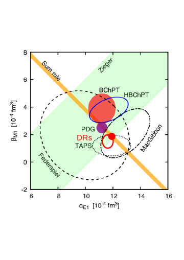
Figure 1: The scalar polarizabilities of the proton. The orange band is the average over the Baldin sum rule evaluations listed in Table 1. The green band shows the experimental constraint on the difference $\alpha_{E1}-\beta_{M1}$ of the dipole polarizabilities from Zieger et al. [58]. The black curves give the experimental results from Federspiel et al. [59], MacGibbon et al. [60], and TAPS [33]. The BChPT result is from Ref. [56] and the HBChPT constraint is from Ref. [54]. The red closed and open circles show the results from the fit using subtracted DRs, with and without the constraint of the Baldin sum rule, respectively [61]. The plot is adapted from Ref. [62].

The optimal strategy would be to use all these constants as fit parameters to the Compton observables. In practice, a simultaneous fit of all the six leading static polarizabilities has not been feasible so-far due to the limited statistics of the available RCS data set.

As a matter of fact, analyses based on subtracted DRs have started to be available only recently, while traditionally the most used analysis tool has been unsubtracted DRs. Figure 1 shows a summary of the extraction of the scalar polarizabilities obtained in various frameworks, using data for the unpolarized RCS cross section below threshold. The experimental fits shown by black curves have been obtained within unsubtracted DRs [15, 33]. Recently, covariant baryon chiral perturbation theory (BChPT) [56] and heavy baryon chiral perturbation theory (HBChPT) [54] have been developed as a convenient framework to analyze RCS data up to the $\Delta$-resonance region. The corresponding fits are shown by the brown disk and blue curve, respectively, and yield values for the magnetic polarizabilities larger than the fits with DRs. The results from the analysis of HBChPT [54] was recently also included in the PDG average (violet disk), resulting in the following values [63]:

$$\alpha_{E1}=(11.2\pm 0.4)\times 10^{-4}\,\mathrm{fm}^{3},\quad\beta_{M1}=(2.5\mp 0.4)\times 10^{-4}\,\mathrm{fm}^{3}.$$ (21)

Finally we quote the results from a recent fit within subtracted DRs [61], which uses as input the MAID07 pion-photoproduction multipoles [45], and the values for the spin polarizabilities extracted from double polarization RCS measurements at MAMI [64]. They have been obtained with and without the constraint of the Baldin sum rule, corresponding respectively to the closed and open red disks in Figure 1:

$$\alpha_{E1} = (11.91\pm 0.22)\times 10^{-4}\,\mathrm{fm}^{3},\,\,\beta_{M1}=(1.86\mp 0.22)\times 10^{-4}\,\,\mathrm{fm}^{3}\,\mathrm{(w/}\,\mathrm{Baldin}\,\mathrm{SR)},$$ (22)

$$\alpha_{E1} = (11.63\pm 0.38)\times 10^{-4}\,\mathrm{fm}^{3},\,\,\beta_{M1}=(1.49\pm 0.48)\times 10^{-4}\,\,\mathrm{fm}^{3}\,\mathrm{(w/o}\,\mathrm{Baldin}\,\mathrm{SR)}.$$ (23)

These results clearly show that the tension for $\beta_{M1}$ between the fits within effective field theories and DRs persists. One should also note that the various fits in Figure 1 have been obtained using different data sets. For example, Ref. [54] has defined an “improved” data set, where a few data points from different experiments have been discarded, whereas the fit with subtracted DRs includes the “full” data set consisting of all available data for the unpolarized RCS cross section below threshold, i.e., the more recent data of Refs. [33, 58, 59, 60, 65] as well as the older data listed in [61]. Preliminary studies of the statistical consistency of the different data subsets show that the fit results may depend on the choice of the data set [61, 66], and therefore the comparison between various fits is not conclusive at the moment. Future measurements planned at MAMI [67] and at the High Intensity Gamma-Ray Source (HI$\gamma$S) [68] hold the promise to clarify this situation. In particular, measurements are underway at MAMI [69] of both the unpolarized cross section and beam asymmetry, with the aim to extract the proton scalar polarizabilities with unprecedented precision from a single experiment. First results of the beam asymmetry with lower statistics provide a proof-of-principle that the scalar polarizabilities can be accessed in this way [70].

In contrast to the scalar polarizabilities, much less is known for the spin polarizabilities. In addition to the results for the FSP from the GGT sum rule discussed in Section 2.1, the experimental value for the backward spin polarizability $\gamma_{\pi}$ has been obtained by an analysis with unsubtracted DRs of backward angle Compton scattering. The average value from three measurements at MAMI (TAPS [33], LARA [71, 72], and SENECA [73]) yields:

$$\gamma_{\pi}=(8.0\pm 1.8)\times 10^{-4}\,\mathrm{fm}^{4}.$$ (24)

To obtain information on the individual spin polarizabilities, one has to resort to double polarization experiments. A systematic study of the sensitivity to the individual polarizabilities of the unpolarized and double polarized Compton observables, with beam and target polarizations, has been performed using subtracted DRs [20], and has been used to plan the double-polarization experimental program at MAMI [74]. More recently, this analysis has been complemented by a study using BChPT [75]. In Table 2 we show the results from the fit, within subtracted DRs, of the recent MAMI measurements [64] for the double polarization asymmetry using circularly polarized photons and transversely polarized proton target ($\Sigma_{2x}$) along with the data for the beam asymmetry either from the LEGS experiment ($\Sigma_{3}^{{\rm LEGS}}$) [76] or from the recent MAMI experiment ($\Sigma_{3}^{{\rm MAMI}}$) [70]. These data have been analyzed to extract the spin polarizabilities $\gamma_{E1E1}$ and $\gamma_{M1M1}$, while the remaining leading static polarizabilities were constrained within the uncertainties of the available experimental results. In particular, the scalar polarizabilities were taken from the 2012 PDG values [77], i.e. $\alpha_{E1}=(12.16\pm 0.58)\cdot 10^{-4}$ fm³ and $\beta_{M1}=(1.66\pm 0.69)\cdot 10^{-4}$ fm³, $\gamma_{0}$ from the GDH & A2 value in Table 1 and $\gamma_{\pi}$ from the experimental value 24. The data for $\Sigma_{2x}$ and $\Sigma_{3}^{{\rm LEGS}}$ have also been analyzed in [64] within BChPT, giving values compatible, within uncertainties, with the DR fit. This is a positive indication that the model dependence of the polarizability fitting is comparable to, or smaller than, the statistical errors of the data. In Table 2 we also report the predictions of unsubtracted DRs, obtained by evaluating the non-Born amplitudes in Eq. 18 at $\nu=t=0$ with the MAID07 input, and the calculations within HBChPT [54], BChPT [56] and a chiral Lagrangian approach (L_χ) [78]. The uncertainties in the fit values are still too large to discriminate between the various approaches. Further analyses, with an unconstrained fit of all the six leading static polarizabilities, including the MAMI measurements for the beam asymmetry [69] and double-polarization asymmetry with circularly polarized photons and longitudinally polarized target [74], hold the promise to pin down the values for the individual spin polarizabilities with better precision.

Table 2: Results for the static spin polarizabilities (in units of $10^{-4}$ fm⁴) from the fit with subtracted DRs to $\Sigma_{2x}$ [67, 64] along with either $\Sigma_{3}^{{\rm LEGS}}$ [76] (first column) or $\Sigma_{3}^{{\rm MAMI}}$ (second column), in comparison with predictions from unsubtracted DRs with the MAID07 input, HBChPT [54], BChPT [56] and a chiral Lagrangian (L_χ) [78].

	$\Sigma_{2x}$ and $\Sigma_{3}^{{\rm LEGS}}$	$\Sigma_{2x}$ and $\Sigma_{3}^{{\rm MAMI}}$	DRs	HBChPT	BChPT	Lχ
$\gamma_{E1E1}$	$-3.5\pm 1.2$	$-5.0\pm 1.5$	$-4.5$	$-1.1\pm 1.8$	$-3.3\pm 0.8$	$-3.7$
$\gamma_{M1M1}$	$3.16\pm 0.85$	$3.13\pm 0.88$	3.0	$2.2\pm 0.7$a	$2.9\pm 1.5$	2.5
$\gamma_{E1M2}$	$-0.7\pm 1.2$	$1.7\pm 1.7$	$-0.08$	$-0.4\pm 0.4$	$0.2\pm 0.2$	1.2
$\gamma_{M1E2}$	$1.99\pm 0.29$	$1.26\pm 0.43$	2.3	$1.9\pm 0.4$	$1.1\pm 0.3$	1.2

^a An additional error of $\pm 0.5$ comes from the fit of the $\gamma N\Delta$ coupling constant to RCS data [54].

2.3 Dynamical polarizabilities

Dynamical polarizabilities combine the concepts of multipole expansion of the scattering amplitudes and nucleon polarizabilities and provide a better filter for the mechanisms governing the nucleon response in Compton scattering. They are functions of the excitation energy and encode the dispersive effects of $\pi N$, $N^{*}$ and other higher intermediate states [16, 79, 80]. The information encoded in the dynamical nucleon polarizabilities has been pointed out in different theoretical calculations, using DRs or effective field theories [52, 79, 80]. However, extracting these polarizabilities from RCS data is very challenging, because of the very low sensitivity of the RCS data to the higher-order dispersive coefficients and the strong correlations between the fit parameters. Work in this direction has been presented recently in [61], where first information on the scalar dynamical dipole polarizabilities (DDPs) has been extracted from RCS data below threshold. The theoretical framework for such analysis relies on the multipole expansion of the scattering amplitude, the LEX of the DDPs, and subtracted DRs for the calculation of the higher-order multipole amplitudes. The statistical analysis was performed using a new method based on the bootstrap technique, that turned out to be crucial to deal with problems inherent to both the low sensitivity of the RCS cross section to the energy dependence of the DDPs and to the limited accuracy of the available data sets. The results of such analysis are shown in Figure 2 (red solid curve), with $68\%$ (yellow) and $95\%$ (green) confidence level (C.L.) uncertainty bands. They have been obtained using two different data sets, i.e., the full data set and the data set given by the TAPS experiment alone [33], which is, by far, the most comprehensive available subset.

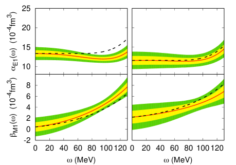
Figure 2: Results from the fit of the DDPs (red solid line) as function of the cm photon energy $\omega$, using the full data set (left panels) and the TAPS subset (right panels): $\alpha_{E1}(\omega)$ on the top and $\beta_{M1}(\omega)$ on the bottom, with the $68\%$ (yellow) and $95\%$ (green) C.L. areas. The dashed lines are predictions from subtracted DRs, with the values at $\omega=0$ fixed to the fit results. Figure from Ref. [61].

The fit results are compared with the subtracted DR predictions [80] (dashed curves) using the MAID07 input [45]. At zero energy, one recovers the value of the static electric and magnetic dipole polarizabilities. At energy $\omega\lesssim 60$ MeV the DR results are within the $68\%$ confidence area of the fit results for all the DDPs. At higher energies, the DR predictions for $\beta_{M1}(\omega)$ remain within the $95\%$ C.L. region, while for $\alpha_{E1}(\omega)$ we observe deviations from the fit results in the case of the full data set and a very good agreement, within the $68\%$ confidence area, in the case of the TAPS data set. This different behavior can be a hint of inconsistencies between the two data sets. The larger error bands in the case of $\beta_{M1}(\omega)$ also reflect the lower sensitivity of the unpolarized RCS data to the magnetic as compared to the electric polarizability. The high-precision measurements planned at MAMI below pion-production threshold [69] will definitely help to disentangle with better accuracy the effects of the individual leading-order static and higher-order dispersive polarizabilities.

3 Virtual Compton scattering

Virtual Compton scattering (VCS) is formally obtained from RCS by replacing the incident real photon with a virtual photon $\gamma^{*}$, and can be accessed experimentally as a subprocess of the reaction $e(k)+N(p)\rightarrow e(k^{\prime})+N(p^{\prime})+\gamma(q^{\prime})$, where the real final photon can be emitted by either the electron or the nucleon. The first process corresponds to the Bethe-Heitler (BH) contribution, which is well known and entirely calculable from QED with the nucleon electromagnetic form factors as input. The second one contains, in the one-photon exchange approximation, the VCS subprocess. The VCS contribution can be further decomposed in a Born term, where the intermediate state is a nucleon as defined in [21], and a non-Born term, which contains all nucleon excitations and meson-loop contributions. At low energy $q^{\prime}$ of the emitted photons, one can use the LET for VCS [21, 81, 6], which states that the non-Born term starts at order $q^{\prime}$, whereas the Born term enters at $1/q^{\prime}$. If we parametrize the non-Born term with a multipole expansion in the cm of the $\gamma^{*}N$ system, the leading contribution in $q^{\prime}=|\boldsymbol{q}^{\prime}|_{{\rm cm}}$ can be expressed in terms of generalized polarizabilities (GPs) with the multipolarities of the emitted photon corresponding to electric and magnetic dipole radiation. For a dipole transition in the final state and arbitrary three-momentum $q=|\boldsymbol{q}|_{{\rm cm}}$ of the virtual photon, angular momentum and parity conservation lead to ten GPs [21], depending on the virtuality $Q^{2}$ of the virtual photon. By further imposing nucleon crossing and charge conjugation symmetry, the number of independent GPs reduces to six [82]. They correspond to two scalar GPs, $\alpha_{E1}(Q^{2})$ and $\beta_{M1}(Q^{2})$, reducing to the RCS static scalar polarizabilities in the limit of $Q^{2}\rightarrow 0$, and four spin-dependent GPs, denoted as [22]:

$$P^{(L1,L1)1}(Q^{2}),\quad P^{(M1,M1)1}(Q^{2}),\quad P^{(M1,L2)1}(Q^{2}),\quad P^{(L1,M2)1}(Q^{2}).$$ (25)

In this notation, $P^{(\rho^{\prime}\ell^{\prime},\rho\ell)1}$ corresponds with a multipole amplitude where $\rho=L,M$ denotes whether the photon is of longitudinal or magnetic type and $\ell$ denotes the angular momentum (respectively, $\rho^{\prime}\ell^{\prime}$ or $\rho\ell$ for the final or initial photon); the index $1$ at the end indicates that the transition involves a nucleon spin flip. In the limit $Q^{2}\rightarrow 0$, the first two spin GPs in Eq. 25 vanish, whereas the latter two reduce to the RCS spin polarizabilities as [83]:

$$\gamma_{E1M2}=-\alpha_{\mathrm{em}}\frac{3}{\sqrt{2}}\,P^{(L1,M2)1}(0),\quad\gamma_{M1E2}=-\alpha_{\mathrm{em}}\frac{3\sqrt{3}}{2\sqrt{2}}\,P^{(M1,L2)1}(0),$$ (26)

where $\alpha_{\mathrm{em}}\equiv e^{2}/4\pi\simeq 1/137$ denotes the fine-structure constant.

According to the LET, the LEX of the VCS observables provides a method to analyze VCS experiments below pion-production threshold in terms of structure functions which contain information on GPs [21, 22]. However, the sensitivity of the VCS cross section to the GPs is enhanced in the region between pion-production threshold and the $\Delta$-resonance region. The LEX does not hold in this regime, but the dispersive approach is expected to give a reasonable framework to extract the GPs. To set up the DR formalism, we can parametrize the non-Born contribution to the VCS scattering amplitude in terms of twelve independent amplitudes $F_{i}(Q^{2},\nu,t),\,i=1,\dots,12$, free of kinematical singularities and constraints and even in $\nu$ [24]. Furthermore, the GPs are expressed in terms of the non-Born part $F^{NB}_{i}$ at the point $t=-Q^{2}$ and $\nu=0$. Assuming an appropriate analytic and high-energy behavior, these amplitudes fulfil unsubtracted DRs in the variable $\nu$ at fixed $t$ and fixed $Q^{2}$:

$$\mathrm{Re}\,F^{NB}_{i}(Q^{2},\nu,t)=F_{i}^{pole}(Q^{2},\nu,t)-F^{B}_{i}(Q^{2},\nu,t)+\frac{2}{\pi}\mathcal{P}\int_{\nu_{thr}}^{+\infty}{\rm d}\nu^{\prime}\frac{\nu^{\prime}\mathrm{Im}\,F_{i}(Q^{2},\nu^{\prime},t)}{\nu^{\prime 2}-\nu^{2}},$$ (27)

where $F_{i}^{B}$ is the Born contribution as defined in [21, 22], whereas $F_{i}^{pole}$ denote the nucleon pole contributions. Furthermore, $\mathrm{Im}\,F_{i}$ are the discontinuities across the $s$-channel cuts, starting at the pion production threshold $\nu_{thr}=m_{\pi}+(m_{\pi}^{2}+t/2+Q^{2}/2)/(2M)$.

The validity of the unsubtracted DRs in Eq. 27 relies on the assumption that at high energies ($\nu\rightarrow\infty$, fixed $t$ and fixed $Q^{2}$) the amplitudes drop fast enough such that the integrals converge. The high-energy behavior of the amplitudes $F_{i}$ was investigated in [23, 24], with the finding that the integrals diverge for $F_{1}$ and $F_{5}$. As long as we are interested in the energy region up to the $\Delta$-resonance, we may saturate the $s$-channel dispersion integral by the $\pi N$ contribution, setting the upper limit of integration to $\nu_{max}=1.5$ GeV. The remainder can be estimated by energy-independent functions, which parametrize the asymptotic contribution due to $t$-channel poles, as well as the residual dispersive contributions beyond the value $\nu_{max}=1.5$ GeV. The asymptotic contribution to $F_{5}$ is saturated by the $\pi^{0}$ pole [24]. The asymptotic contribution to $F_{1}$ can be described phenomenologically as the exchange of an effective $\sigma$ meson, in the same spirit as for unsubtracted DRs in the RCS case. The $Q^{2}$ dependence of this term is unknown. It can be parametrized in terms of a function directly related to the magnetic dipole GP $\beta_{M1}(Q^{2})$ and fitted to VCS observables. Furthermore, it was found that the unsubtracted DR for the amplitude $F_{2}$ is not so well saturated by $\pi N$ intermediate states only. The additional $s$-channel contributions beyond the $\pi N$ states can effectively be accounted for with an energy-independent function, at fixed $Q^{2}$ and $t=-Q^{2}$. This amounts to introducing an additional fit function, which is directly related to the electric dipole GP $\alpha_{E1}(Q^{2})$. In order to provide predictions for VCS observables, it is convenient to adopt the following parametrizations for the fit functions:

$$\alpha_{E1}(Q^{2})-\alpha_{E1}^{\pi N}(Q^{2})=\frac{\alpha_{E1}^{exp}-\alpha_{E1}^{\pi N}}{(1+Q^{2}/\Lambda_{\alpha}^{2})^{2}},\quad\beta_{M1}(Q^{2})-\beta_{M1}^{\pi N}(Q^{2})=\frac{\beta_{M1}^{exp}-\beta_{M1}^{\pi N}}{(1+Q^{2}/\Lambda_{\beta}^{2})^{2}},$$ (28)

where $\alpha_{E1}$ and $\beta_{M1}$ are the RCS polarizabilities, with superscripts $exp$ and $\pi N$ indicating, respectively, the experimental value and the $\pi N$ contribution evaluated from unsubtracted DRs. In Eq. 28, the mass scale parameters $\Lambda_{\alpha}$ and $\Lambda_{\beta}$ are free parameters, not necessarily constant with $Q^{2}$, which can be adjusted by a fit to the experimental cross sections.

A series of VCS measurements at MAMI [84, 85, 86, 87, 88, 89, 90], JLab  [91, 92], and Bates [93, 94] have provided a first experimental exploration of the proton’s electric and magnetic GPs. These experiments involve measurements below and above pion threshold, and results have been extracted using both the LEX and DR approaches. A fundamental difference between the two analysis methods is that the DR formalism allows for a direct extraction of the scalar GPs, by fitting the parameters $\Lambda_{\alpha}$ and $\Lambda_{\beta}$ to the data, whereas the LEX analysis gives access to structure functions depending linearly on both scalar and spin GPs [21]. In order to disentangle the scalar GPs, the contribution from the spin GPs to the structure functions has to be subtracted using a model. One usually uses the DR model, introducing some model dependence which is presently not accounted for in the error bars. Figure 3 displays the results for the electric GP, $\alpha_{E1}(Q^{2})$, and the magnetic GP, $\beta_{M1}(Q^{2})$, from the world VCS measurements, showing a nice consistency between the LEX and DR extractions. The solid curves correspond to the DR predictions, obtained with the PDG values of Eq. 21 for the static polarizabilities at $Q^{2}=0$ and the mass scales $\Lambda_{\alpha}=0.73$ GeV and $\Lambda_{\beta}=0.63$ GeV. The dashed curves are the predictions from BChPT [95], which are plotted in the low-$Q^{2}$ range of applicability of the theory and without the theory-uncertainty band.

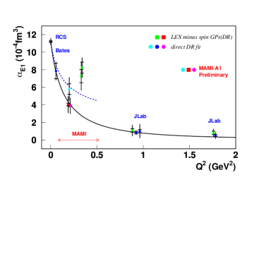
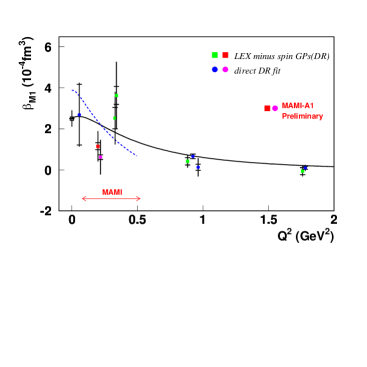
Figure 3: Compilation of world data for $\alpha_{E1}(Q^{2})$ (left) and $\beta_{M1}(Q^{2})$ (right) at different $Q^{2}$ values in GeV²: $Q^{2}=0$ from the PDG values, Eq. 21; $Q^{2}=0.06$ from MIT-Bates [94, 93]; $Q^{2}=0.33$ from MAMI [84, 86]; $Q^{2}=0.2$ from the preliminary analysis of MAMI  [88, 89, 90]; $Q^{2}=0.92,1.76$ from JLab [91, 92]. Solid curves: DR predictions, with mass scales $\Lambda_{\alpha}=0.73$ GeV and $\Lambda_{\beta}=0.63$ GeV. Dashed curves: BChPT predictions [95]. Plot courtesy of H. Fonvieille.

One notices from Figure 3 that the electric GP, which is dominated by the asymptotic contribution, cannot be described by a single dipole form over the full $Q^{2}$ range. In particular, the data situation near $Q^{2}=0.3$ GeV² is currently not understood, since all the models, such as chiral effective field theories [96, 97, 98, 99, 100, 95], the linear-$\sigma$ model [101, 102], non-relativistic [103, 104] and relativistic [105] constituent quark models, predict a smooth fall-off with $Q^{2}$. The magnetic GP results from a large dispersive $\pi N$ (paramagnetic) contribution, dominated by $\Delta(1232)$ resonance, and a large asymptotic (diamagnetic) contribution with opposite sign, leading to a relatively small net result with a relatively flat behavior at low $Q^{2}$. We also note the difference at low $Q^{2}$ between the DR and BChPT predictions, which are not resolved by the existing experimental data. More high-precision measurements are needed, and the new experimental data from MAMI [88] at $Q^{2}=0.1$ and $0.45$ GeV² together with the upcoming measurements at JLab [106] in the $Q^{2}$ range of 0.3-0.75 GeV² should mark a step forward in our understanding of the underlying mechanisms which govern the structure of the GPs at low and intermediate $Q^{2}$.

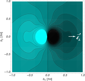
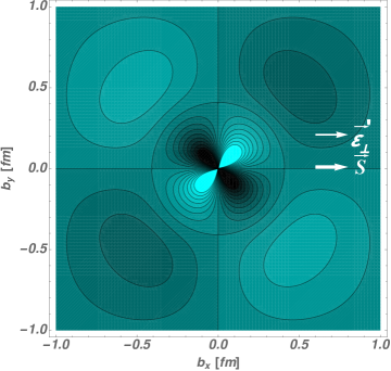
Figure 4: Induced polarization density in a proton of definite light-cone helicity (left), and with spin $\boldsymbol{S}$ along the $x$-axis (right), when submitted to an electromagnetic field with photon polarization along the $x$-axis, as indicated. Light (dark) regions correspond to the largest (smallest) values.

A precise knowledge of the $Q^{2}$ dependence of the GPs is crucial to obtain, through a Fourier transform, a spatial representation of the deformation of the charge and magnetization distributions of the nucleon under the influence of an external static electromagnetic field [107, 108]. A proper spatial-density interpretation can be formulated by considering the nucleon in a light-front frame [108]. In this frame, the two transverse components $\boldsymbol{q}_{\perp}$ of the virtual photon momentum, with $Q^{2}=\boldsymbol{q}_{\perp}^{2}$, are the conjugate variables to the transverse position coordinates $\boldsymbol{b}_{\perp}$ of the quarks in a nucleon. Furthermore, the polarization vector $\boldsymbol{\epsilon}^{\prime}_{\perp}$ of the outgoing photon is associated with an external quasi-static electromagnetic field, polarizing the charge and magnetization distributions. Such polarization densities are described by different scalar and spin GPs, depending on the spin state of the nucleon. In Figure 4 we show the polarization densities in transverse-position space for a proton in a definite light-front helicity state (left panel) and for a proton in an eigenstate of the transverse-spin $\boldsymbol{S}$ (right panel), as calculated using the DR results of the GPs shown in Figure 3. In the former case, the polarization density displays a dipole pattern dominated by the scalar GPs, with the spatial extension at the nucleon periphery strongly depending on the mass scale $\Lambda_{\alpha}$. In the second case, on top of a weak dipole deformation, we observe a quadrupole pattern with pronounced strength around 0.5 fm due to the electric GP.

4 Forward double virtual Compton scattering

In this section, we review the application of DRs to the forward double VCS (VVCS) process:

$$\gamma^{\ast}(q)+N(p)\to\gamma^{\ast}(q)+N(p),$$ (29)

where both photons have the same finite space-like virtuality $q^{2}=-Q^{2}\leq 0$. We discuss the resulting LEX for the VVCS amplitudes and sum rules in terms of generalized, i.e. $Q^{2}$ dependent, polarizabilities. For the polarized VVCS amplitude, we discuss two model-independent relations at low $Q^{2}$, connecting moments of spin structure functions to polarizabilities accessible in RCS and VCS, as discussed in Sections 2 and  3 respectively. For the unpolarized VVCS amplitude involving transverse virtual photons, one subtraction function is required. We discuss the information on the $Q^{2}$ dependence of this subtraction function in terms of polarizabilities and chiral effective field theories.

The forward VVCS tensor $M^{\mu\nu}$, with $\mu$ $(\nu)$ denoting the four-vector index of initial (final) photon, is described by four invariant amplitudes, denoted by $T_{1},T_{2},S_{1},S_{2}$, which are functions of $Q^{2}$ and $\nu\equiv p\cdot q/M$, as [109]:

$$\alpha_{em}\,M^{\mu\nu} = \left(g^{\mu\nu}-\frac{q^{\mu}q^{\nu}}{q^{2}}\right)T_{1}(\nu,Q^{2})-\frac{1}{M^{2}}\left(p^{\mu}-\frac{p\cdot q}{q^{2}}\,q^{\mu}\right)\left(p^{\nu}-\frac{p\cdot q}{q^{2}}\,q^{\nu}\right)T_{2}(\nu,Q^{2})$$ (30)

$$- \frac{i}{M}\epsilon^{\nu\mu\alpha\beta}\,q_{\alpha}s_{\beta}\,S_{1}(\nu,Q^{2})-\frac{i}{M^{3}}\epsilon^{\nu\mu\alpha\beta}\,q_{\alpha}(p\cdot q\ s_{\beta}-s\cdot q\ p_{\beta})\,S_{2}(\nu,Q^{2}),$$

where $\epsilon_{0123}=+1$, $s^{\alpha}$ is the nucleon covariant spin vector satisfying $s\cdot p$ = 0, $s^{2}=-1$. Note that this definition implies that at the real photon point the amplitudes $T_{1}$ and $S_{1}$ are related to the amplitudes $f$ and $g$ of Eq. 3, describing the forward RCS, as: $T_{1}(\nu,0)=f(\nu)$ and $S_{1}(\nu,0)=(M/\nu)g(\nu)$.

The optical theorem yields the following relations for the imaginary parts of the four amplitudes appearing in Eq. 30:

$${\rm{Im}}\ T_{1}(\nu,\,Q^{2})=\frac{e^{2}}{4M}F_{1}(x,\,Q^{2})\, \quad{\rm{Im}}\ T_{2}(\nu,\,Q^{2})=\frac{e^{2}}{4\nu}F_{2}(x,\,Q^{2})\,,$$ ,

$${\rm{Im}}\ S_{1}(\nu,\,Q^{2})=\frac{e^{2}}{4\nu}g_{1}(x,\,Q^{2})\, \quad{\rm{Im}}\ S_{2}(\nu,\,Q^{2})=\frac{e^{2}}{4}\frac{M}{\nu^{2}}g_{2}(x,\,Q^{2})\,,$$ , (31)

where $x\equiv Q^{2}/(2M\nu)$ is the Bjorken variable, and $F_{1},F_{2},g_{1},g_{2}$ are the conventionally defined structure functions which parametrize inclusive electron-nucleon scattering. The imaginary parts of the forward scattering amplitudes, Eqs. 4, get contributions from both elastic scattering at $\nu=\nu_{B}\equiv Q^{2}/(2M)$ or equivalently $x=1$, as well as from inelastic processes above pion threshold, corresponding with $\nu>\nu_{thr}\equiv m_{\pi}+(Q^{2}+m_{\pi}^{2})/(2M)$ or equivalently $x<x_{thr}\equiv\nu_{B}/\nu_{thr}$. The elastic contributions are obtained as pole parts of the direct and crossed nucleon Born diagrams. The latter are conventionally separated off the Compton scattering tensor in order to define structure dependent constants, such as polarizabilities. The Born terms are given by [18]:

$$T_{1}^{B} = -\frac{\alpha_{\mathrm{em}}}{M}(F_{D}^{2}+\frac{\nu_{B}^{2}}{\nu^{2}-\nu_{B}^{2}+i\varepsilon}\,G_{M}^{2})\,,\quad T_{2}^{B}=-\frac{\alpha_{\mathrm{em}}}{M}\,\frac{Q^{2}}{\nu^{2}-\nu_{B}^{2}+i\varepsilon}\,(F_{D}^{2}+\tau\,F_{P}^{2})\,,$$

$$S_{1}^{B} = -\frac{\alpha_{\mathrm{em}}}{2M}(F_{P}^{2}+\frac{Q^{2}}{\nu^{2}-\nu_{B}^{2}+i\varepsilon}\,F_{D}G_{M})\,,\quad S_{2}^{B}=\frac{\alpha_{\mathrm{em}}}{2}\frac{\nu}{\nu^{2}-\nu_{B}^{2}+i\varepsilon}\,F_{P}G_{M}\,,$$ (32)

where $\tau\equiv Q^{2}/4M^{2}$, and $F_{D}$ and $F_{P}$ are the Dirac and Pauli form factors (FFs) of the nucleon $N$, normalized to $F_{D}(0)=e_{N}$ and $F_{P}(0)=\kappa_{N}$. Furthermore, the magnetic FF combination is given by $G_{M}\,(Q^{2})=F_{D}\,(Q^{2})+F_{P}(Q^{2})$. From the Born contributions of Eq. 32 one can directly read off the nucleon pole contributions.

We next consider the analyticity in $\nu$, for fixed $Q^{2}$, of the VVCS amplitudes. We can distinguish two cases depending on the symmetry in the $s-u$ crossing variable $\nu$: $T_{1},T_{2}$, and $S_{1}$ are even functions of $\nu$ whereas $S_{2}$ is an odd function of $\nu$. We discuss DRs for the non-pole parts of the amplitudes, i.e., when subtracting the well known pole contributions from the full amplitudes. In particular, we will consider unsubtracted DRs for the spin dependent amplitudes $S_{1}$ and $S_{2}$, and will then discuss the spin independent amplitudes, of which $T_{1}$ will require one subtraction. We will concentrate within the scope of this review on the model independent results at low $Q^{2}$. For a discussion of sum rules and of nucleon spin structure at larger $Q^{2}$, we refer the reader e.g. to the reviews of [18, 25, 26].

4.1 Spin dependent VVCS sum rules

An unsubtracted DR for the non-pole ($np$) part of the amplitude $S_{1}$ is given by:

$${\rm{Re}}\,S_{1}^{np}(\nu,\,Q^{2})\,=\,2\alpha_{\mathrm{em}}\,{\mathcal{P}}\,\int_{\nu_{thr}}^{\infty}\,d\nu^{\prime}\,\frac{1}{\nu^{\prime\,2}-\nu^{2}}\,\,g_{1}(x^{\prime},\,Q^{2}),$$ (33)

with $x^{\prime}\equiv\nu_{B}/\nu^{\prime}$. For a fixed finite value of $Q^{2}$, the LEX in $\nu$ for $S_{1}^{np}$ (and analogously for $S_{2}^{np}$) can be expressed through the inelastic odd moments of the structure functions $g_{1}$ ($g_{2}$), defined as:

$$\Gamma_{1,2}^{(n)\,inel}(Q^{2}) \equiv \int_{0}^{x_{thr}}\,dx\,x^{(n-1)}\,g_{1,2}\,(x,\,Q^{2}),\quad n=1,3,5,...$$ (34)

For $S_{1}^{np}$, the LEX takes the form [29, 18]:

$$S_{1}^{np}(\nu,\,Q^{2})=\frac{2\,\alpha_{\mathrm{em}}}{M}\,I_{1}(Q^{2})+\left[\frac{2\,\alpha_{\mathrm{em}}}{\nu_{B}^{3}}\Gamma_{1}^{(3)\,inel}(Q^{2})\right]\,\nu^{2}\,+\,{\mathcal{O}}(\nu^{4}),$$ (35)

where we have re-expressed the lowest moment as:

$$I_{1}(Q^{2}) \;\equiv\; \frac{M}{\nu_{B}}\,\Gamma_{1}^{(1)\,inel}(Q^{2}),$$ (36)

which yields the GDH sum rule value at $Q^{2}=0$: $I_{1}(0)=-\kappa_{N}^{2}/4$. Furthermore at $Q^{2}=0$, the term of ${\mathcal{O}}(\nu^{2})$ in Eq. (35) yields the FSP as: $\left[(2\alpha_{\mathrm{em}}/\nu_{B}^{3})\Gamma_{1}^{(3)\,inel}(Q^{2})\right]_{Q^{2}=0}=M\gamma_{0}$. One can derive further sum rules by Taylor expanding Eq. 35 for $S_{1}^{np}$ in $Q^{2}$ at $\nu=0$. In this way, the following extension of the GDH sum rule to finite $Q^{2}$ was obtained in [110, 111] for the slope at $Q^{2}=0$ of the moment $I_{1}(Q^{2})$:

$$I_{1}^{\prime}(0)\equiv\frac{dI_{1}}{dQ^{2}}\bigg{|}_{Q^{2}=0}=\frac{\kappa_{N}^{2}}{12}\langle r_{2}^{2}\rangle+\frac{M^{2}}{2}\left\{\frac{\gamma_{E1M2}}{\alpha_{\mathrm{em}}}-3M\left[P^{\prime(M1,M1)1}(0)+P^{\prime(L1,L1)1}(0)\right]\right\}.$$ (37)

All quantities entering Eq. 37 are observable quantities: the lhs is obtained from the first moment of the spin structure function $g_{1}$, whereas the rhs involves the squared Pauli radius $\langle r_{2}^{2}\rangle$ as well as spin polarizabilities measured through the RCS and VCS processes, and introduced in Sections 2 and 3.

For the second spin-dependent VVCS amplitude $S_{2}$, which is odd in $\nu$, an unsubtracted DR takes the form:

$${\rm{Re}}\,S_{2}(\nu,\,Q^{2})\,=\,2\alpha_{\mathrm{em}}M\nu\,{\mathcal{P}}\,\int_{0}^{\infty}d\nu^{\prime}\frac{1}{\nu^{\prime\,2}-\nu^{2}}\,\frac{1}{\nu^{\prime\,2}}\,g_{2}(x^{\prime},\,Q^{2})\,,$$ (38)

where the nucleon-pole contribution is included in the integral on the rhs. If we further assume that the amplitude $S_{2}$ converges faster than $1/\nu$ for $\nu\rightarrow\infty$, we may write an unsubtracted DR for the amplitude $\nu\,S_{2}$, which is even in $\nu$,

$${\rm{Re}}\left[\nu\,S_{2}(\nu,\,Q^{2})\right]\,=\,2\alpha_{\mathrm{em}}M\,{\mathcal{P}}\,\int_{0}^{\infty}\,d\nu^{\prime}\,\frac{1}{\nu^{\prime\,2}-\nu^{2}}\,g_{2}(x^{\prime},\,Q^{2})\,.$$ (39)

By multiplying Eq. 38 by $\nu$ and subtracting it from Eq. 39, one then obtains the Burkhardt-Cottingham (BC) “superconvergence sum rule” [27], valid for any value of $Q^{2}$:

$$\int_{0}^{1}\,g_{2}\,(x,\,Q^{2})\,dx=0,$$ (40)

provided that the integral converges for $x\rightarrow 0$. The upper integration limit in Eq. 40 extends to $1$, and thus includes the elastic (i.e. pole) contribution. By separating elastic and inelastic parts in the integral of Eq. 40, the BC sum rule can be expressed equivalently:

$$\Gamma_{2}^{(1)\,inel}(Q^{2})\,=\,\frac{\nu_{B}}{4M}\,F_{P}(Q^{2})G_{M}(Q^{2}).$$ (41)

In perturbative QCD, the BC sum rule was verified for a quark target to first order in $\alpha_{s}$ [112]. In the non-perturbative domain of low $Q^{2}$, the BC sum rule was also verified within HBChPT [113, 114].

The LEX of the non-pole part of the amplitude $(\nu S_{2})$ in Eq. 39 can be expressed as [18]:

$$\left[\nu\,S_{2}(\nu,\,Q^{2})\right]^{np}=\frac{2\alpha_{\mathrm{em}}M}{\nu_{B}}\,\Gamma_{2}^{(1)\,inel}(Q^{2})\,+\,\left[\frac{2\alpha_{\mathrm{em}}M}{\nu_{B}^{3}}\Gamma_{2}^{(3)\,inel}(Q^{2})\right]\,\nu^{2}\,+\,{\mathcal{O}}(\nu^{4})\,.$$ (42)

The third moments of the spin structure functions $g_{1}$ and $g_{2}$ can be combined by defining a longitudinal-transverse polarizabilitiy $\delta_{LT}(Q^{2})$ as [18]:

$$\delta_{LT}\,(Q^{2}) \;\equiv\; \frac{2\,\alpha_{\mathrm{em}}}{M\nu_{B}^{3}}\,\left\{\Gamma_{1}^{(3)\,inel}(Q^{2})+\Gamma_{2}^{(3)\,inel}(Q^{2})\right\}.$$ (43)

By Taylor expanding $(\nu S_{2})^{np}$ in $Q^{2}$, a further sum rule was obtained in [110, 111] for the term in Eq. 42 proportional to $\nu^{2}$ at $Q^{2}=0$, yielding the polarizability $\delta_{LT}(0)$ as:

$$\delta_{LT}(0)=-\gamma_{E1E1}+3M\alpha_{\mathrm{em}}\,\left[P^{\prime\,(M1,M1)1}(0)-P^{\prime\,(L1,L1)1}(0)\right].$$ (44)

Note that similar to their counterpart of Eq. 37, all quantities which enter Eq. 44 are observables in RCS or VCS, therefore providing a model independent and predictive relation among low-energy spin structure constants of the nucleon.

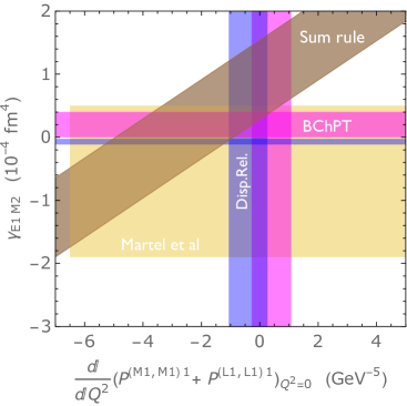
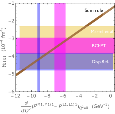
Figure 5: The sum rules of Eq. 37 (left panel) and Eq. 44 (right panel) between proton spin polarizabilities in RCS and VCS respectively. Left: the brown band is the sum rule constraint based on the empirical information for $I_{1}^{\prime}(0)$ from JLab/CLAS [115, 116], and for $\langle r_{2}^{2}\rangle$ from [117]. Right: the brown band is the sum rule constraint based on the phenomenological MAID2007 [45] information for $\delta_{LT}(0)$. The yellow bands are the empirical extraction from [64]. The purple bands are the DR evaluations [18] for the RCS and VCS polarizabilities, where the width of the bands is obtained by using either MAID2000 [44] or MAID2007 [45] as input in the dispersive evaluations. The pink bands are the BChPT evaluations ($\pi N+\Delta+\pi\Delta$) [118, 56, 95]. Figure from Ref. [111].

We provide a graphical presentation of the spin dependent sum rules of Eqs. 37 and 44 in Figure 5. Using only the empirical information for $I_{1}^{\prime}(0)$ and $\delta_{LT}(0)$, the sum rules yield a slanted (brown) band in the plots of $\gamma_{E1M2}$ and $\gamma_{E1E1}$ versus the slopes of the GPs. The pioneering experimental values for $\gamma$’s, obtained by the A2 Coll. at MAMI [64], are shown by the broad horizontal (yellow) bands. The region where the two bands overlap gives a prediction for the slopes of the GPs. A measurement of GP slopes using VCS is required to directly verify this prediction. One furthermore sees that the phenomenological DR estimates of Ref. [18] as well as the results obtained in BChPT are well in agreement, within uncertainties, with the RCS spin polarizabilities and are consistent with the sum rule bands. The BChPT results for the slopes of the two spin GPs are also in relatively good agreement with the DR estimates, as noted in Ref. [95].

Furthermore, ChPT calculations allow to make predictions for the low $Q^{2}$ dependence of different moments of spin structure functions as given e.g. in Eqs. 36 or 43. Besides early calculations within HBChPT [119, 113, 114], in more recent years two variants of BChPT have been developed, yielding predictions for different spin structure function moments at low $Q^{2}$ [120, 118]. Although the earlier data [25, 26] only covered the larger $Q^{2}$ range, where the theory may lose its predictive power, very recent data [116, 121] and data currently under analysis [122, 123] will allow to quantitatively test the predictions of ChPT for the moments of proton and neutron spin structure functions for $Q^{2}$ down to $0.01$ GeV².

4.2 Spin independent VVCS sum rules

We next turn to the spin-independent VVCS amplitudes entering Eq. 30. Their non-Born parts, denoted by $T^{NB}_{1}$ and $T^{NB}_{2}$, were recently expressed, including all terms up to fourth order in $k=\{Q,\nu\}$, as [109]:

$$T^{NB}_{1}(\nu,Q^{2}) = Q^{2}\,\beta_{M1}+\nu^{2}\,(\alpha_{E1}+\beta_{M1})+\nu^{4}\left[\alpha_{E1\nu}+\beta_{M1\nu}+\frac{1}{12}(\alpha_{E2}+\beta_{M2})\right]$$ (45)

$$+ Q^{2}\nu^{2}\left[\beta_{M1\nu}+\frac{1}{12}(4\beta_{M2}+\alpha_{E2})+2(\alpha^{\prime}_{E1}(0)+\beta^{\prime}_{M1}(0))-\alpha_{\mathrm{em}}8M^{2}b_{4,1}\right.$$

$$+ \left.\frac{1}{M}\left(-\delta_{LT}(0)+\gamma_{M1M1}-\gamma_{E1E1}-\gamma_{M1E2}+\gamma_{E1M2}\right)+\frac{1}{(2M)^{2}}(\alpha_{E1}+\beta_{M1})\right]$$

$$+ Q^{4}\,\left[\frac{1}{6}\beta_{M2}+2\beta^{\prime}_{M1}(0)+\alpha_{\mathrm{em}}b_{3,0}+\frac{1}{(2M)^{2}}\beta_{M1}\right]+{\cal O}(k^{6}),$$

$$T^{NB}_{2}(\nu,Q^{2}) = Q^{2}\,(\alpha_{E1}+\beta_{M1})+Q^{2}\nu^{2}\left[\alpha_{E1\nu}+\beta_{M1\nu}+\frac{1}{12}(\alpha_{E2}+\beta_{M2})\right]$$ (46)

$$+ Q^{4}\left[\frac{1}{6}(\alpha_{E2}+\beta_{M2})+2(\alpha^{\prime}_{E1}(0)+\beta^{\prime}_{M1}(0))-\alpha_{\mathrm{em}}\,4M^{2}b_{19,0}\right.$$

$$\left.-\frac{1}{M}\left(\delta_{LT}(0)+\gamma_{E1E1}+\gamma_{M1E2}\right)+\frac{1}{(2M)^{2}}(\alpha_{E1}+\beta_{M1})\right]+{\cal O}(k^{6}).$$

We notice that the quadratic terms are fully determined by the proton electric ($\alpha_{E1}$) and magnetic ($\beta_{M1}$) dipole polarizabilities. The terms of order $\nu^{4}$ in $T^{NB}_{1}$ and of order $Q^{2}\nu^{2}$ in $T^{NB}_{2}$ are also fully determined by the electric and magnetic dispersive and quadrupole polarizabilities which are observables in RCS. The terms of order $Q^{2}\nu^{2}$ in $T^{NB}_{1}$ and of order $Q^{4}$ in $T^{NB}_{2}$ involve in addition the slopes $\alpha^{\prime}_{E1}(0)$ and $\beta^{\prime}_{M1}(0)$ at $Q^{2}=0$ of the electric and magnetic GPs, shown in Fig. 3, as well as the RCS spin polarizabilities and the longitudinal-transverse spin polarizability $\delta_{LT}(0)$, all of which are also observable quantities either through RCS, VCS, or using moments of spin structure functions. The only unknowns in these $Q^{2}\nu^{2}$ terms arise from the low-energy coefficients $b_{4,1}$ and $b_{19,0}$, as defined through the expansion for the VVCS used in [109]. We will next show that two forward sum rules will allow to also fix these constants. The remaining low-energy constant, $b_{3,0}$ appears at order $Q^{4}$ in $T^{NB}_{1}$, and is determined from the $Q^{2}$ dependence of the subtraction term in this amplitude, as discussed below.

The DR for the non-pole part $T_{1}^{np}$ of the VVCS amplitude $T_{1}$ requires one subtraction, which we take at $\nu=0$, in order to ensure high-energy convergence:

$${\rm{Re}}T_{1}^{np}(\nu,\,Q^{2})\, = \,T_{1}^{np}(0,\,Q^{2})+\frac{2\alpha_{\mathrm{em}}\,\nu^{2}}{M}\,{\mathcal{P}}\,\int_{\nu_{thr}}^{\infty}\,d\nu^{\prime}\,\frac{1}{\nu^{\prime}(\nu^{\prime\,2}-\nu^{2})}\,F_{1}(x^{\prime},Q^{2}).$$ (47)

The LEX of the non-pole part $T_{1}^{np}$, at fixed $Q^{2}$, takes the form [18]:

$$T_{1}^{np}(\nu,\,Q^{2})\, = T_{1}^{np}(0,\,Q^{2})\,+\,M^{(2)}_{1}(Q^{2})\,\nu^{2}\,+\,M^{(4)}_{1}(Q^{2})\,\nu^{4}\,+\,{\mathcal{O}}(\nu^{6})\,,$$ (48)

where $M^{(2)}_{1}(Q^{2})$ and $M^{(4)}_{1}(Q^{2})$ can respectively be expressed through the second and fourth moments of the unpolarized nucleon structure function $F_{1}$ as:

$$M^{(2)}_{1}(Q^{2})=\frac{2\alpha_{\mathrm{em}}}{M\nu_{B}^{2}}\int_{0}^{x_{thr}}dx^{\prime}x^{\prime}F_{1}(x^{\prime},Q^{2}),\quad M^{(4)}_{1}(Q^{2})=\frac{2\alpha_{\mathrm{em}}}{M\nu_{B}^{4}}\int_{0}^{x_{thr}}dx^{\prime}x^{\prime\,3}F_{1}(x^{\prime},Q^{2}).$$ (49)

To connect the LEX of the non-Born part $T_{1}^{NB}$ of Eq. 45 with Eq. 48, we also need to account for the difference between the Born and pole parts. As the difference between the Born and pole term contributions to $T_{1}$ is independent of $\nu$ it can be fully absorbed in the subtraction function $T_{1}(0,Q^{2})$, see Ref. [109] for details.

The $\nu$-dependent terms in the expansion of Eq. 48 can then all be determined from sum rules in terms of electro-absorption cross sections on a nucleon. The terms of order $\nu^{2}$ ($\nu^{4}$) in the LEX of Eq. 45 yield at $Q^{2}=0$ respectively the Baldin sum rule of Eq. 9 and its higher-order generalization of Eq. 10 as:

$$M^{(2)}_{1}(0)=\alpha_{E1}+\beta_{M1},\quad\quad M^{(4)}_{1}(0)=\alpha_{E1,\nu}+\beta_{M1,\nu}+\frac{1}{12}(\alpha_{E2}+\beta_{M2}).$$ (50)

The term proportional to $Q^{2}\nu^{2}$ in the LEX of Eq. 45, yields a new sum rule [109]:

$$M^{(2)\prime}_{1}(0) \equiv \frac{dM^{(2)}_{1}}{dQ^{2}}\bigg{|}_{Q^{2}=0}=\beta_{M1,\nu}+\frac{1}{12}(4\beta_{M2}+\alpha_{E2})+2(\alpha^{\prime}_{E1}(0)+\beta^{\prime}_{M1}(0))-\alpha_{\mathrm{em}}8M^{2}b_{4,1}$$ (51)

$$+\frac{1}{M}\left(-\delta_{LT}+\gamma_{M1M1}-\gamma_{E1E1}-\gamma_{M1E2}+\gamma_{E1M2}\right)+\frac{1}{(2M)^{2}}(\alpha_{E1}+\beta_{M1}).\quad$$

The structure function moment $M^{(2)}_{1}(Q^{2})$ is an observable which has been measured at JLab/Hall C [124]. One can then use the measured value on the lhs of the sum rule of Eq. 51 in order to determine the low-energy coefficient $b_{4,1}$.

For the amplitude $T_{2}$, which is even in $\nu$, one can write an unsubtracted DR in $\nu$ :

$${\rm{Re}}T_{2}^{np}(\nu,\,Q^{2})\,=\,2\alpha_{\mathrm{em}}\,{\mathcal{P}}\,\int_{\nu_{thr}}^{\infty}\,d\nu^{\prime}\,\frac{1}{\nu^{\prime\,2}-\nu^{2}}\,F_{2}(x^{\prime},\,Q^{2})\,.$$ (52)

For the amplitude $T_{2}$ there is no difference between the Born and pole contributions, and its LEX expansion can be directly read off Eq. 46, and expressed as:

$$T_{2}^{np}(\nu,\,Q^{2})\, = M^{(2)}_{1}(0)\,Q^{2}+M^{(4)}_{1}(0)\,Q^{2}\nu^{2}+M^{(1)\prime}_{2}(0)\,Q^{4}+\,{\mathcal{O}}(k^{6}).$$ (53)

One recovers from the $Q^{2}$ term the Baldin sum rule, and from the $Q^{2}\nu^{2}$ term the higher-order Baldin sum rule. Furthermore, the term of order $\mathcal{O}(Q^{4})$ involves the derivative at $Q^{2}=0$ of the first moment of the structure function $F_{2}$, defined as:

$$M^{(1)}_{2}(Q^{2}) = \frac{\alpha_{\mathrm{em}}}{M\nu_{B}^{2}}\,\int_{0}^{x_{thr}}dx^{\prime}\,F_{2}(x^{\prime},\,Q^{2}),$$ (54)

which satisfies $M_{2}^{(1)}(0)=M_{1}^{(2)}(0)$. Its derivative at $Q^{2}=0$ can then be obtained from Eq. 46 through the sum rule relation [109]:

$$M^{(1)\prime}_{2}(0)\equiv\frac{dM^{(1)}_{2}(Q^{2})}{dQ^{2}}\bigg{|}_{Q^{2}=0} = \frac{1}{6}(\alpha_{E2}+\beta_{M2})+2(\alpha^{\prime}_{E1}(0)+\beta^{\prime}_{M1}(0))-\alpha_{\mathrm{em}}\,4M^{2}b_{19,0}$$ (55)

$$- \frac{1}{M}\left(\delta_{LT}+\gamma_{E1E1}+\gamma_{M1E2}\right)+\frac{1}{(2M)^{2}}(\alpha_{E1}+\beta_{M1}).$$

The knowledge of the slope $M^{(1)\prime}_{2}(0)$, which is an observable, allows to determine the low-energy coefficient $b_{19,0}$.

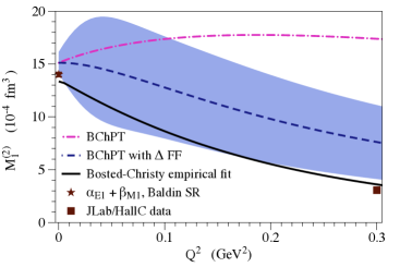
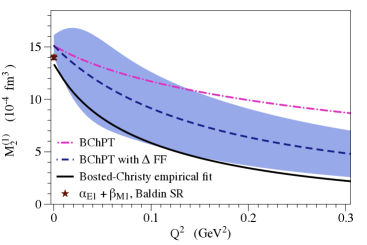
Figure 6: $Q^{2}$ dependence of the proton structure moments $M^{(2)}_{1}$ (left) and $M^{(1)}_{2}$ (right) according to the empirical Bosted-Christy fit (black solid curve) [125], in comparison with the $\pi N+\Delta+\pi\Delta$ BChPT calculation [109]. For the latter, the blue dashed (magenta dashed-dotted) curves show the results with (without) an additional FF dependence in the $\Delta$-exchange, respectively. The blue band shows the uncertainty of the BChPT result with the FF, estimated as in [95]. At the real photon point, both observables yield the Baldin sum rule value for $\alpha_{E1}+\beta_{M1}$ [30]. The data point at $Q^{2}=0.3$ GeV² (left panel) is from JLab/HallC [124]. Figure from Ref. [109].

Figure 6 shows the empirical Bosted-Christy fits [125] for the moments $M_{1}^{(2)}$ and $M_{2}^{(1)}$ in the low-$Q^{2}$ region, and compares them with the $\pi N+\Delta+\pi\Delta$ BChPT calculation of Ref. [109]. One can notice that the BChPT curves agree, within their (rather wide) error bands, with the empirical fit results. One can see that the use of FFs in the $\gamma N\Delta$ vertex is an important part of this result.

In order to completely fix the term of $\mathcal{O}(Q^{4})$ in the subtraction function $T_{1}^{NB}(0,Q^{2})$, one needs to determine the low-energy coefficient $b_{3,0}$. Its determination requires a measurement of the VVCS process with a spacelike initial and timelike final photon, which is not available at present. As its determination is of importance in the leading hadronic corrections to the proton radius extraction from muonic Lamb shift measurements, we will compare the behavior of $T_{1}^{NB}(0,Q^{2})$ in different approaches. Figure 7 compares $T^{NB}_{1}(0,Q^{2})/Q^{2}$ as obtained in BChPT and HBChPT [126], with a superconvergence relation estimate [127]. At the real photon point, $T^{NB}_{1}(0,Q^{2})/Q^{2}$ is given by the magnetic dipole polarizability $\beta_{M1}$. The superconvergence and HBChPT estimates were fixed at $Q^{2}=0$ to the PDG value for $\beta_{M1}$ of Eq. 21, whereas the BChPT estimate reflects the larger value for $\beta_{M1}$ in this framework. One notices from Figure 7 that in the BChPT result, the inclusion of the $\gamma N\Delta$ FF yields a suppression at non-zero $Q^{2}$, yielding a zero crossing in the $Q^{2}$ range between $0.05-0.25$ GeV². A negative value for $T_{1}^{NB}(0,Q^{2})$ at intermediate $Q^{2}$ values is also obtained in the empirical superconvergence estimate [127].

A further observable requiring the knowledge of the subtraction function, is the electromagnetic mass difference between proton and neutron, involving an integral in $Q^{2}$ of the $T_{1}^{NB}(0,Q^{2})$ difference for proton and neutron, see Refs. [128, 129] for some recent works.

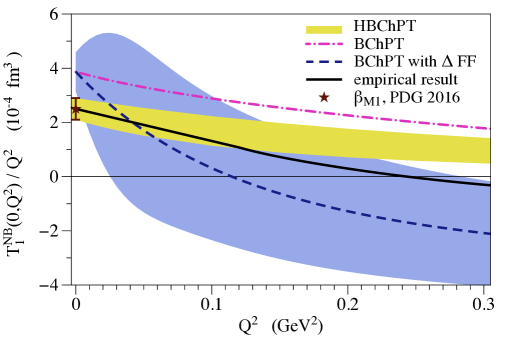
Figure 7: The low-$Q^{2}$ behavior of the non-Born part of the subtraction function $T_{1}^{NB}(0,Q^{2})$ divided by $Q^{2}$. The dark yellow band is the HBChPT result [126]. The blue dashed (magenta dashed-dotted) curves show the BChPT calculation of [109] with (without) $\gamma N\Delta$ FF respectively. The blue band shows the uncertainty of the BChPT result with $\gamma N\Delta$ FF, estimated in [95]. The black solid curve shows the empirical superconvergence relation estimate of [127]. At the real photon point, the PDG value for $\beta_{M1}$ of Eq. 21 is shown. Note that the HBChPT curve was shifted to reproduce that value. Figure from Ref. [109].

5 Polarizability corrections to muonic hydrogen spectroscopy

In this section we discuss how the phenomenological information on the unpolarized forward VVCS of the last section is used in estimates of the two-photon exchange (TPE) corrections to the Lamb shift in muonic atoms. The recent extractions of the proton charge radius from the Lamb shift measurements in muonic hydrogen [130, 131] resulted in a significant discrepancy in comparison with measurements with electrons [132, 117, 133], see Refs. [131, 134, 135] for recent reviews. In view of this discrepancy, the higher-order corrections to the Lamb shift were examined in detail by many groups. In particular, the TPE proton structure corrections were scrutinized over the past decade, see Ref. [62] for a review and references therein. The TPE correction contributes at present the largest theoretical uncertainty when extracting the charge radius from the Lamb shift data, thus limiting its accuracy. In this Section, we briefly review the current status of the dispersive estimates as used in the muonic hydrogen Lamb shift analyses [136] and compare them with the model independent ChPT analyses.

The $n$-th $S$-level shift in the (muonic) hydrogen spectrum due to forward TPE is related to the spin-independent VVCS amplitudes [137] as:

$$\Delta E^{\mathrm{TPE}}(nS)=8\pi e^{2}m\phi_{n}^{2}\frac{1}{i}\int_{-\infty}^{\infty}\!\frac{d\nu}{2\pi}\int\!\!\frac{d\vec{q}}{(2\pi)^{3}}\frac{\left(Q^{2}-2\nu^{2}\right)T_{1}(\nu,Q^{2})-(Q^{2}+\nu^{2})\,T_{2}(\nu,Q^{2})}{Q^{4}(Q^{4}-4m^{2}\nu^{2})},$$ (56)

where $m$ is the lepton mass, $\phi_{n}^{2}=(\alpha_{\mathrm{em}}m_{r}/n)^{3}/\pi$ is the wave function at the origin, with $m_{r}$ the reduced mass of the lepton-proton system. The polarizability effect on the hydrogen spectrum is described by the non-Born amplitudes $T^{NB}_{1}$ and $T^{NB}_{2}$ . This polarizability effect can be split into the contribution of the subtraction function $T^{NB}_{1}(0,Q^{2})$ [138, 137]:

$$\Delta E^{\mathrm{subtr.}}(nS)=8m\alpha_{\mathrm{em}}\phi_{n}^{2}\,\int_{0}^{\infty}\frac{dQ}{Q^{3}}\frac{v_{l}+2}{(1+v_{l})^{2}}\,T^{NB}_{1}(0,Q^{2}),$$ (57)

with $v_{l}=\sqrt{1+4m^{2}/Q^{2}}$, and contributions of the inelastic structure functions [62]:

$$\Delta E^{\mathrm{inel.}}(nS) = -32\alpha_{\mathrm{em}}^{2}Mm\,\phi_{n}^{2}\,\int_{0}^{\infty}\frac{dQ}{Q^{5}}\,\int_{0}^{x_{thr}}dx\frac{1}{(1+v_{l})(1+\sqrt{1+x^{2}\tau^{-1}})}$$ (58)

$$\times\Bigg{\{}\left[1+\frac{v_{l}\sqrt{1+x^{2}\tau^{-1}}}{v_{l}+\sqrt{1+x^{2}\tau^{-1}}}\right]F_{2}(x,Q^{2})$$

$$+\frac{2x}{(1+v_{l})(1+\sqrt{1+x^{2}\tau^{-1}})}\left[2+\frac{3+v_{l}\sqrt{1+x^{2}\tau^{-1}}}{v_{l}+\sqrt{1+x^{2}\tau^{-1}}}\right]F_{1}(x,Q^{2})\Bigg{\}}.$$

The sum of Eqs. 57 and 58 is referred to as the total polarizability contribution.

Table 3 shows the TPE corrections due to the inelastic structure functions estimate of [137] and resulting from the subtraction-function estimate of [126], both of which are currently used in estimating the total polarizability contribution to the $2S$-level in the muonic hydrogen analyses [136]. The estimate of [126] assumes a dipole ansatz for $T_{1}^{NB}(0,Q^{2})/Q^{2}$, and constrains the mass parameter by a HBChPT calculation to fourth-order in the chiral expansion for the $Q^{4}$ term in $T_{1}^{NB}(0,Q^{2})$. We compare these results with a LO BChPT analysis, a NLO BChPT analysis which includes the $\Delta$-pole contribution, and with the NLO HBChPT analysis of [139]. One notices that the BChPT result which includes the $\Delta$-pole is in very good agreement with the DR estimate for the inelastic contribution and with the estimate of [126] for the subtraction function contribution. It is also interesting that, although the $\Delta$-pole contributes sizeably to both terms, these contributions come with opposite sign, resulting in a small total polarizability contribution due to the $\Delta$-pole, and a total result close to the LO BChPT estimate. In Table 3, we also show a NLO HBChPT estimate [139] (last column). Even though it comes with a larger error estimate, its value is larger (in magnitude), deviating by about $2\sigma$ from the BChPT and DR estimates. It was noticed however [139], that the inclusion of the nucleon Born term contributions yields a total TPE result which is similar in size as the DR and BChPT results.

Table 3: TPE corrections to the 2$S$-level in muonic hydrogen. All values are given in $\mu$eV. The first two rows are the dispersive ($\Delta E^{\mathrm{inel.}}$) and subtraction function ($\Delta E^{\mathrm{subtr.}}$) contributions. The sum of both yields the total polarizability contribution ($\Delta E^{\mathrm{pol.}}$).

	DR + HBChPT	BChPT (LO)	BChPT (LO + $\Delta$)	HBChPT (NLO)
	[137, 126, 136]	[140]	[109]	[139]
$\Delta E^{\mathrm{inel.}}$	$-12.7\pm 0.5$   [137]	$-5.2$	$-11.8$	$-$
$\Delta E^{\mathrm{subtr.}}$	$4.2\pm 1.0$   [126]	$-3.0$	$4.6$	$-$
$\Delta E^{\mathrm{pol.}}$	$-8.5\pm 1.1$   [136]	$-8.2^{+1.2}_{-2.5}$	$-7.2^{+1.2}_{-2.5}$	$-26.2\pm 10.0$

Although the TPE contribution is at present the largest theoretical uncertainty when extracting the proton charge radius from the muonic hydrogen Lamb shift, its total size, as obtained from both DRs and ChPT, is approximately one-tenth as large as would be needed to explain the observed discrepancy in the proton charge radius extraction from electronic or muonic observables, thus leaving the ”proton radius puzzle” unresolved [137]. The TPE correction is also by far the largest theoretical uncertainty when analyzing the hyperfine splitting in the muonic hydrogen, in this case resulting from the polarized proton structure functions $g_{1}$ and $g_{2}$. We refer to [62] for a recent review of the status of this field.

6 Conclusions and Outlook

Dispersion relations (DRs) are a powerful tool to extract information on hadron structure constants from analyses of electromagnetic processes. We have reviewed the real and virtual Compton scattering off the proton and summarized the recent advances in the DR analyses applied to such processes. We discussed the latest evaluations of forward real Compton scattering (RCS) sum rules. We furthermore reviewed the application of both unsubtracted and subtracted DR approaches to the non-forward RCS process as tools to extract the proton polarizabilities. The comparison between the fits within DRs and alternative fits within chiral perturbation theories (ChPTs) clearly shows tension for $\beta_{M1}$, which may depend on the different choice of the database used in the analyses. We also discussed recent advances in a multipole analysis of RCS data, along with a recent DR fit of the energy-dependent dynamical polarizabilities. We subsequently reviewed the application of DRs to the virtual Compton scattering (VCS) process, and discussed the world data on the generalized polarizabilities (GPs) extracted from such process. Apart from some conflicting data situation in the electric GP around $Q^{2}=0.3$ GeV² which remains to be sorted out, the VCS world data have allowed to extract the $Q^{2}$ dependence of the GPs up to values of around $2$ GeV². We have discussed how these data allow to map out the spatial distribution of the polarization densities in a proton. Furthermore, we have reviewed new sum rules for the forward double-virtual Compton scattering (VVCS) process on a nucleon, which allow for model-independent relations between polarizabilities in RCS, VCS, and moments of nucleon structure functions. We have presented the status of these sum rules, using both empirical DR evaluations and baryon ChPT. Finally, we have reviewed how this information is used to predict and constrain the polarizability corrections to muonic hydrogen spectroscopy.

We end this review by spelling out a few open issues and challenges (both theoretical and experimental) in this field:

1. Scalar and spin polarizabilities in RCS: Ongoing experiments at MAMI with transversely and longitudinally polarized targets, and a circularly polarized photon beam, as well as with unpolarized targets and a linearly polarized beam, aim to improve the determination of proton polarizabilities. Much of the data has already been acquired, and the analyses of the polarized data are nearly completed [67]. A first experiment with a linearly polarized photon beam [70] has demonstrated a proof of principle for a independent determination of $\beta_{M1}$ from such data. A longer run, with improvements in both the tagging system and the linear beam polarization stability, is underway. This run will provide both a reduction in the asymmetry errors by a factor of about 3.5 and a set of cross-section measurements, that together will enable a separate extraction of $\alpha_{E1}$ and $\beta_{M1}$ at level of the PDG errors [67]. At HI$\gamma$S [68], RCS data has recently been taken on the differential cross section and beam asymmetry at photon lab energy of $85$ MeV at three different scattering angles, and is presently being analyzed. Further measurements below threshold with transversely polarized target and circularly polarized photon are planned.

2. Dynamical polarizabilities in RCS: The improved statistics and precision of the upcoming data set for the unpolarized cross section and beam asymmetry will definitely help to determine with better accuracy the effects of the leading-order static and dynamical polarizabilities. In order to also include the data above pion threshold in the analysis, a full dispersive treatment for the fit of the dynamical polarizabilities should be developed, by giving up the low-energy expansion of the multipole amplitudes used in the recent analysis of Ref. [61].

3. Generalized polarizabilities in VCS: New data on the unpolarized VCS response functions and GPs have been taken at MAMI and are currently in a final stage of analysis. These data will complement the $Q^{2}=0.2$ GeV² points [89] shown in this work. In particular, expected are data at $Q^{2}=0.1$ GeV² and $Q^{2}=0.45$ GeV², which are in the domain of applicability of BChPT, and will further test the theoretical predictions. A newly approved experiment at JLab [106] which plans to measure the unpolarized GPs in the $Q^{2}$ range of $0.3-0.75$ GeV² will be able to shed further light on the conflicting data situation around $Q^{2}=0.3$ GeV². Furthermore, unpolarized VCS data at the same $Q^{2}$ value for different beam energies allows to separate off the VCS response function labeled $P_{TT}$, which contains only spin GPs. This will allow one to experimentally access, for the first time, the dominant spin GP $P^{(M1,M1)1}$ and provide a strong test of the BChPT and DR predictions.

4. Further developments of the dispersion formalism: As the subtracted DR approach for RCS requires the input from the $t$-channel discontinuities, it can be further improved by a refined analysis of the leading $\gamma\gamma\to\pi\pi$ channel in view of new data for this channel. Furthermore, a better control of the analytical continuation of the $s$-channel contribution into the unphysical region will allow to extend the formalism to energies around the $\Delta$-resonance region at larger value of $-t$ (backward angles). An aim for the VCS process, where currently only an unsubtracted DR formalism has been developed, is to develop a subtracted DR formalism along the lines of the subtracted DR framework for RCS. To this aim, it will be necessary to have the dispersive input of the $\gamma^{\ast}\gamma\to\pi\pi$ channel.

5. Spin structure functions at low $Q^{2}$: Data on the deuteron spin structure function moments of $g_{1}$ at low $Q^{2}$, down to $0.02$ GeV², have recently become available from the JLab/Hall B EG4 experiment [121]. The same experiment also measured the proton spin structure function moments of $g_{1}$ at low $Q^{2}$, down to $0.01$ GeV², which are currently under analysis. Data on the proton spin structure function $g_{2}$, using a polarized proton target, are also forthcoming from the JLab/Hall C SANE experiment [122] and from the JLab/Hall A g2p experiment [123]. In both cases, the data analysis is in an advanced stage. Together with the existing data on the neutron spin structure functions, the combined data set will allow for a definitive test of the ChPT results for the low $Q^{2}$ spin structure function moments.

6. Subtraction function $T_{1}(0,Q^{2})$ in unpolarized VVCS: Extending the knowledge of this key quantity, which enters both the two-photon exchange (TPE) correction to muonic atoms as well as the electromagnetic mass difference between proton and neutron, beyond the region where ChPT predictions are applicable, is clearly of high interest. Superconvergence estimates [129, 127] for the VVCS subtraction function $T_{1}(0,Q^{2}$) in the $Q^{2}\lesssim 2$ GeV² region are currently constrained by nucleon structure function data in the resonance region ($W<3$ GeV) as well as by HERA data at high energies ($W>10$ GeV). However, in the intermediate $W$ region ($3\lesssim W\lesssim 10$ GeV), the empirical estimates are quite uncertain due to the scarce data situation in that region. Forthcoming structure function data from the JLab 12 GeV program will allow to further improve such estimates, and extract the VVCS low-energy constant $b_{3,0}$. It may also be very worthwhile to directly access $b_{3,0}$ through a low-energy VVCS experiment, using the $e^{-}+p\to e^{-}+p+l^{-}l^{+}$ process by measuring a dilepton pair ($l^{-}l^{+}$) in the final state.

7. Polarizability corrections to muonic atom energy levels: Although the theoretical precision of two-photon exchange (TPE) corrections to the muonic hydrogen Lamb shift is currently at the level of the experimental one, the situation still needs to be improved for dispersive TPE estimates for muonic deuterium [141] or muonic ${}^{3}He^{+}$ [142] in order to match the experimental precisions. New data on few-body electromagnetic observables from the MESA facility in Mainz [143] hold the promise to provide the required input. Furthermore, forthcoming high-precision experiments by the CREMA [144] and FAMU [145] collaborations, and at J-PARC [146] aim to measure the 1S hyperfine splitting in muonic hydrogen to a level of precision of $1~{}\mathrm{ppm}$, exceeding by around two orders of magnitude the current theoretical precision. As the latter is limited by the knowledge of the low $Q^{2}$ proton’s elastic form factors and spin structure functions, further studies to improve on their measurements are warranted.

DISCLOSURE STATEMENT

The authors are not aware of any affiliations, memberships, funding, or financial holdings that might be perceived as affecting the objectivity of this review.

References

- [1] Kronig R. J. opt. Soc. Amer. 12:547 (1926)
- [2] Kramers HA. Atti Congr. Intern. Fisici, Como 2:545 (1927)
- [3] Gell-Mann M, Goldberger ML, Thirring W. Phys. Rev. 95:1612 (1954)
- [4] Goldberger ML. Phys. Rev. 97:508 (1955)
- [5] Gell-Mann M, Goldberger ML. Phys. Rev. 96:1433 (1954)
- [6] Low FE. Phys. Rev. 96:1428 (1954)
- [7] Abarbanel HDI, Goldberger ML. Phys. Rev. 165:1594 (1968)
- [8] Klein A. Phys. Rev. 99:998 (1955)
- [9] Baldin AM. Nucl. Phys. 18:310 (1960)
- [10] Gerasimov SB. Sov. J. Nucl. Phys. 2:430 (1966), [Yad. Fiz.2,598(1965)]
- [11] Drell SD, Hearn AC. Phys. Rev. Lett. 16:908 (1966)
- [12] Akiba T, Sato I. Progr. Theoret. Phys. 19:93 (1958)
- [13] Lapidus LI, Chou KC. Soviet Phys.-JETP 11:147 (1960)
- [14] Holliday D. Ann. Phys. (N.Y.) 24:289 (1963)
- [15] L’vov AI, Petrun’kin VA, Schumacher M. Phys. Rev. C55:359 (1997)
- [16] Babusci D, et al. Phys. Rev. C58:1013 (1998)
- [17] Drechsel D, Gorchtein M, Pasquini B, Vanderhaeghen M. Phys. Rev. C61:015204 (1999)
- [18] Drechsel D, Pasquini B, Vanderhaeghen M. Phys. Rept. 378:99 (2003)
- [19] Schumacher M. Prog. Part. Nucl. Phys. 55:567 (2005)
- [20] Pasquini B, Drechsel D, Vanderhaeghen M. Phys. Rev. C76:015203 (2007)
- [21] Guichon PAM, Liu GQ, Thomas AW. Nucl. Phys. A591:606 (1995)
- [22] Guichon PAM, Vanderhaeghen M. Prog. Part. Nucl. Phys. 41:125 (1998)
- [23] Pasquini B, et al. Phys. Rev. C62:052201 (2000)
- [24] Pasquini B, et al. Eur. Phys. J. A11:185 (2001)
- [25] Kuhn SE, Chen JP, Leader E. Prog. Part. Nucl. Phys. 63:1 (2009)
- [26] Chen JP. Int. J. Mod. Phys. E19:1893 (2010)
- [27] Burkhardt H, Cottingham WN. Annals Phys. 56:453 (1970)
- [28] Anselmino M, Ioffe BL, Leader E. Sov. J. Nucl. Phys. 49:136 (1989), [Yad. Fiz.49,214(1989)]
- [29] Ji XD, Osborne J. J. Phys. G27:127 (2001)
- [30] Gryniuk O, Hagelstein F, Pascalutsa V. Phys. Rev. D92:074031 (2015)
- [31] Pasquini B, Pedroni P, Drechsel D. Phys. Lett. B687:160 (2010)
- [32] Babusci D, Giordano G, Matone G. Phys. Rev. C57:291 (1998)
- [33] Olmos de Leon V, et al. Eur. Phys. J. A10:207 (2001)
- [34] Ahrens J, et al. Phys. Rev. Lett. 87:022003 (2001)
- [35] Dutz H, et al. Phys. Rev. Lett. 91:192001 (2003)
- [36] Helbing K. Prog. Part. Nucl. Phys. 57:405 (2006)
- [37] Gryniuk O, Hagelstein F, Pascalutsa V. Phys. Rev. D94:034043 (2016)
- [38] Armstrong TA, et al. Phys. Rev. D5:1640 (1972)
- [39] Bartalini O, et al. Phys. Atom. Nucl. 71:75 (2008), [Yad. Fiz.71,76(2008)]
- [40] Sandorfi AM, et at. Report No. BNL-64382 (1996)
- [41] Caldwell DO, et al. Phys. Rev. Lett. 40:1222 (1978)
- [42] Aid S, et al. Z. Phys. C69:27 (1995)
- [43] Chekanov S, et al. Nucl. Phys. B627:3 (2002)
- [44] Drechsel D, Hanstein O, Kamalov SS, Tiator L. Nucl. Phys. A645:145 (1999)
- [45] Drechsel D, Kamalov SS, Tiator L. Eur. Phys. J. A34:69 (2007)
- [46] Workman RL, Briscoe WJ, Paris MW, Strakovsky II. Phys. Rev. C85:025201 (2012)
- [47] Hanstein O, Drechsel D, Tiator L. Nucl. Phys. A632:561 (1998)
- [48] Ahrens J, et al. Phys. Rev. Lett. 84:5950 (2000)
- [49] Holstein BR, Drechsel D, Pasquini B, Vanderhaeghen M. Phys. Rev. C61:034316 (2000)
- [50] Pascalutsa V, Phillips DR. Phys. Rev. C67:055202 (2003)
- [51] Hildebrandt RP, Griesshammer HW, Hemmert TR. Eur. Phys. J. A20:329 (2004)
- [52] Lensky V, Pascalutsa V. Eur. Phys. J. C65:195 (2010)
- [53] Lensky V, McGovern JA, Phillips DR, Pascalutsa V. Phys. Rev. C86:048201 (2012)
- [54] McGovern JA, Phillips DR, Griesshammer HW. Eur. Phys. J. A49:12 (2013)
- [55] Griesshammer HW, McGovern JA, Phillips DR, Feldman G. Prog. Part. Nucl. Phys. 67:841 (2012)
- [56] Lensky V, McGovern JA, Pascalutsa V. Eur. Phys. J. C75:604 (2015)
- [57] Höhler G. vol. I/9b2. Landolt-Börnstein, H. Schopper, Springer (1983)
- [58] Zieger A, et al. Phys. Lett. B278:34 (1992)
- [59] Federspiel FJ, et al. Phys. Rev. Lett. 67:1511 (1991)
- [60] MacGibbon BE, et al. Phys. Rev. C52:2097 (1995)
- [61] Pasquini B, Pedroni P, Sconfietti S arXiv:1711.07401 [hep-ph] (2017)
- [62] Hagelstein F, Miskimen R, Pascalutsa V. Prog. Part. Nucl. Phys. 88:29 (2016)
- [63] Patrignani C, et al. Chin. Phys. C40:100001 (2016)
- [64] Martel PP, et al. Phys. Rev. Lett. 114:112501 (2015)
- [65] Hallin EL, et al. Phys. Rev. C48:1497 (1993)
- [66] Krupina N, Lensky V, Pascalutsa V arXiv:1712.05349 [nucl-th] (2017)
- [67] Martel P, et al. EPJ Web Conf. 142:01021 (2017)
- [68] Weller HR, et al. Prog. Part. Nucl. Phys. 62:257 (2009)
- [69] Downie EJ, et al. Proposal MAMI-A2/04-16 (2016)
- [70] Sokhoyan V, et al. Eur. Phys. J. A53:14 (2017)
- [71] Galler G, et al. Phys. Lett. B503:245 (2001)
- [72] Wolf S, et al. Eur. Phys. J. A12:231 (2001)
- [73] Camen M, et al. Phys. Rev. C65:032202 (2002)
- [74] Hornidge D, et al. Proposal MAMI-A2/05-2012 (2012)
- [75] Griesshammer HW, McGovern JA, Phillips DR arXiv:1711.11546 [nucl-th] (2017)
- [76] Blanpied G, et al. Phys. Rev. C64:025203 (2001)
- [77] Beringer J, et al. Phys. Rev. D86:010001 (2012)
- [78] Gasparyan AM, Lutz MFM, Pasquini B. Nucl. Phys. A866:79 (2011)
- [79] Griesshammer HW, Hemmert TR. Phys. Rev. C65:045207 (2002)
- [80] Hildebrandt RP, Griesshammer HW, Hemmert TR, Pasquini B. Eur. Phys. J. A20:293 (2004)
- [81] Scherer S, Korchin AY, Koch JH. Phys. Rev. C54:904 (1996)
- [82] Drechsel D, et al. Phys. Rev. C57:941 (1998)
- [83] Drechsel D, et al. Phys. Rev. C58:1751 (1998)
- [84] Roche J, et al. Phys. Rev. Lett. 85:708 (2000)
- [85] Bensafa IK, et al. Eur. Phys. J. A32:69 (2007)
- [86] Janssens P, et al. Eur. Phys. J. A37:1 (2008)
- [87] Doria L, et al. Phys. Rev. C92:054307 (2015)
- [88] Merkel H, Fonvieille H. Proposal MAMI-A1/1-09 (2009)
- [89] Correa L. 2016. Measurement of the generalized polarizabilities of the proton by virtual Compton scattering at MAMI and GeV2. Ph.D. thesis, Mainz, Clermont-Ferrand
- [90] Blomberg A. 2016. Low Momentum transfer measurements of pion electroproduction and virtual Compton scattering at the Delta resonance. Ph.D. thesis, Temple U.
- [91] Laveissiere G, et al. Phys. Rev. Lett. 93:122001 (2004)
- [92] Fonvieille H, et al. Phys. Rev. C86:015210 (2012)
- [93] Bourgeois P, et al. Phys. Rev. C84:035206 (2011)
- [94] Bourgeois P, et al. Phys. Rev. Lett. 97:212001 (2006)
- [95] Lensky V, Pascalutsa V, Vanderhaeghen M. Eur. Phys. J. C77:119 (2017)
- [96] Hemmert TR, Holstein BR, Knochlein G, Scherer S. Phys. Rev. D55:2630 (1997)
- [97] Hemmert TR, Holstein BR, Knochlein G, Scherer S. Phys. Rev. Lett. 79:22 (1997)
- [98] Hemmert TR, Holstein BR, Knochlein G, Drechsel D. Phys. Rev. D62:014013 (2000)
- [99] Kao CW, Vanderhaeghen M. Phys. Rev. Lett. 89:272002 (2002)
- [100] Kao CW, Pasquini B, Vanderhaeghen M. Phys. Rev. D70:114004 (2004), [Erratum: Phys. Rev.D92,no.11,119906(2015)]
- [101] Metz A, Drechsel D. Z. Phys. A356:351 (1996)
- [102] Metz A, Drechsel D. Z. Phys. A359:165 (1997)
- [103] Liu GQ, Thomas AW, Guichon PAM. Austral. J. Phys. 49:905 (1996)
- [104] Pasquini B, Scherer S, Drechsel D. Phys. Rev. C63:025205 (2001)
- [105] Pasquini B, Salmè G. Phys. Rev. C57:2589 (1998)
- [106] Paolone M, Sparveris N, Camsonne A, Jones M. Jefferson Lab Experiment C12-15-001
- [107] L’vov AI, et al. Phys. Rev. C64:015203 (2001)
- [108] Gorchtein M, Lorcé C, Pasquini B, Vanderhaeghen M. Phys. Rev. Lett. 104:112001 (2010)
- [109] Lensky V, Hagelstein F, Pascalutsa V, Vanderhaeghen M arXiv:1712.03886 [hep-ph] (2017)
- [110] Pascalutsa V, Vanderhaeghen M. Phys. Rev. D91:051503 (2015)
- [111] Lensky V, Pascalutsa V, Vanderhaeghen M, Kao C. Phys. Rev. D95:074001 (2017)
- [112] Altarelli G, Lampe B, Nason P, Ridolfi G. Phys. Lett. B334:187 (1994)
- [113] Kao CW, Spitzenberg T, Vanderhaeghen M. Phys. Rev. D67:016001 (2003)
- [114] Kao CW, Drechsel D, Kamalov S, Vanderhaeghen M. Phys. Rev. D69:056004 (2004)
- [115] Prok Y, et al. Phys. Lett. B672:12 (2009)
- [116] Fersch R, et al. Phys. Rev. C96:065208 (2017)
- [117] Bernauer JC, et al. Phys. Rev. C90:015206 (2014)
- [118] Lensky V, Alarcón JM, Pascalutsa V. Phys. Rev. C90:055202 (2014)
- [119] Ji XD, Kao CW, Osborne J. Phys. Lett. B472:1 (2000)
- [120] Bernard V, Epelbaum E, Krebs H, Meissner UG. Phys. Rev. D87:054032 (2013)
- [121] Adhikari KP, et al. Phys. Rev. Lett. 120:062501 (2018)
- [122] Kang H. PoS DIS2013:206 (2013)
- [123] Zielinski R. 2010. The g2p Experiment: A Measurement of the Proton’s Spin Structure Functions. Ph.D. thesis, New Hampshire U.
- [124] Liang Y, Christy ME, Ent R, Keppel CE. Phys. Rev. C73:065201 (2006)
- [125] Christy ME, Bosted PE. Phys. Rev. C81:055213 (2010)
- [126] Birse MC, McGovern JA. Eur. Phys. J. A48:120 (2012)
- [127] Tomalak O, Vanderhaeghen M. Eur. Phys. J. C76:125 (2016)
- [128] Walker-Loud A, Carlson CE, Miller GA. Phys. Rev. Lett. 108:232301 (2012)
- [129] Gasser J, Hoferichter M, Leutwyler H, Rusetsky A. Eur. Phys. J. C75:375 (2015)
- [130] Pohl R, et al. Nature 466:213 (2010)
- [131] Antognini A, et al. Science 339:417 (2013)
- [132] Bernauer JC, et al. Phys. Rev. Lett. 105:242001 (2010)
- [133] Mohr PJ, Taylor BN, Newell DB. Rev. Mod. Phys. 84:1527 (2012)
- [134] Carlson CE. Prog. Part. Nucl. Phys. 82:59 (2015)
- [135] Hill RJ. EPJ Web Conf. 137:01023 (2017)
- [136] Antognini A, et al. Annals Phys. 331:127 (2013)
- [137] Carlson CE, Vanderhaeghen M. Phys. Rev. A84:020102 (2011)
- [138] Pachucki K. Phys. Rev. A60:3593 (1999)
- [139] Peset C, Pineda A. Nucl. Phys. B887:69 (2014)
- [140] Alarcón JM, Lensky V, Pascalutsa V. Eur. Phys. J. C74:2852 (2014)
- [141] Carlson CE, Gorchtein M, Vanderhaeghen M. Phys. Rev. A89:022504 (2014)
- [142] Carlson CE, Gorchtein M, Vanderhaeghen M. Phys. Rev. A95:012506 (2017)
- [143] Denig A. AIP Conf. Proc. 1735:020006 (2016)
- [144] Pohl R. J. Phys. Soc. Jap. 85:091003 (2016)
- [145] Adamczak A, et al. JINST 11:P05007 (2016)
- [146] Ma Y, et al. Int. J. Mod. Phys. Conf. Ser. 40:1660046 (2016)