Stress-stress fluctuation formula for elastic constants in the NPT ensemble

Abstract

Several fluctuation formulas are available for calculating elastic constants from equilibrium correlation functions in computer simulations, but the ones available for simulations at constant pressure exhibit slow convergence properties and cannot be used for the determination of local elastic constants. To overcome these drawbacks, we derive a stress-stress fluctuation formula in the $NPT$ ensemble based on known expressions in the $NVT$ ensemble. We validate the formula in the $NPT$ ensemble by calculating elastic constants for the simple nearest-neighbor Lennard-Jones crystal and by comparing the results with those obtained in the $NVT$ ensemble. For both local and bulk elastic constants we find an excellent agreement between the simulated data in the two ensembles. To demonstrate the usefulness of the new formula, we apply it to determine the elastic constants of a simulated lipid bilayer.

I Introduction

The possibility to determine elastic properties of solid and soft materials from computer simulations Ray (1988); Barrat (2006) has significantly advanced our understanding of how non-crystalline materials react under loading. This includes strongly inhomogeneous systems such as glasses Mizuno et al. (2013), polymer fibers Meier (1993) and granular materials Aubouy et al. (2003). Particularly useful is the access to local elastic constants and their spatial variation, which, for example, can provide important information on the change of elastic properties close to interfaces, grain boundaries, and surfaces VanWorkum and de Pablo (2003); Kluge et al. (1990). For obtaining the elastic constants one can directly simulate stress-strain curves by applying small deformations (or stresses) Ray (1988); Griebel and Hamaekers (2004), or analyze equilibrium correlation functions by resorting to the fluctuation-dissipation theorem Ray (1988); Parrinello and Rahman (1982), or introduce phenomenological expressions of free energies with parameters, which can be determined in simulations and related to the constants of the free energy expansion with respect to strain West et al. (2009); Neder et al. (2010).

Most straightforward procedures for calculating elastic constants are the evaluations of proper equilibrium correlation functions in fluctuation formulas (FF). Various approaches with different levels of complexity have been established to this end. Among them, the FF applicable in constant pressure simulations neither exhibit good convergence properties upon averaging nor do they allow one to determine local elastic constants, which are important for the characterization of inhomogeneous materials Barrat (2006); Ganguly et al. (2013). A FF with good convergence properties and access to local elastic constants has been derived for the $NVT$ ensemble Gusev et al. (1996); Lutsko (1988), but no corresponding FF is yet available for the $NPT$ ensemble. The goal of this work is to fill this gap.

After given an overview of the existing methods to calculate elastic constants from FF in Sec. II, we derive the new FF in the $NPT$ ensemble in Sec. III. In Sec. IV we then validate the FF by calculating the elastic constants of the nearest-neighbor Lennard-Jones fcc solid and comparing results with those reported earlier in the literature. We further show that, to obtain well-converged values for the elastic constants, one needs to perform averages over a comparable number of equilibrated particle configurations in the $NPT$ and $NVT$ ensemble. We demonstrate the usefulness of the new FF by determining the elastic constants of a simulated lipid bilayer based on the model developed in Lenz and Schmid (2007) in Sec. V. In this model, the bilayer is stabilized by a surrounding gas of solvent beads, reflecting the pressure exerted by an aqueous environment. Thus, the access to local elastic constants allows us to selectively extract the elastic properties of the lipid bilayer, without the need to modify the most convenient simulation procedure of such a system at constant pressure. As pointed out in the concluding Sec. VI, this possibility will be one of the main advantages of the new FF.

II Fluctuation formulas for elastic constants

For calculating elastic constants in molecular dynamics simulations, a special molecular dynamics ensemble with a fixed external stress tensor $\tau$, the $N\tau T$ ensemble ($N$: number of particles, $T$: temperature) was introduced Parrinello and Rahman (1981). In this ensemble the shape of the simulation cell, and accordingly the instantaneous strain tensor $\epsilon$, is allowed to fluctuate. In general, the pressure is given by the trace of $\tau$, and the special choice $\tau_{\alpha\beta}=-P\delta_{\alpha\beta}$ corresponds to the $NPT$ ensemble. The geometry of the rectilinear simulation cell is described by a scaling matrix $h$, whose columns are the vectors along the edges of the cell. The first order bulk elastic constants $C_{\alpha\beta\mu\nu}$ can be calculated from the strain-strain FF Parrinello and Rahman (1982)

$$C_{\alpha\beta\mu\nu}^{-1}=\frac{k_{\rm\scriptscriptstyle B}T}{\langle V\rangle_{\tau}}\langle\epsilon_{\alpha\beta}\epsilon_{\mu\nu}\rangle_{\tau}\,,$$ (1)

where $k_{\rm\scriptscriptstyle B}$ is the Boltzmann constant, $V$ the instantaneous volume, and $\langle\ldots\rangle_{\tau}$ denotes the average in the $N\tau T$ ensemble; $C_{\alpha\beta\mu\nu}^{-1}$ is the inverse of $C_{\alpha\beta\mu\nu}$ in the sense that $C_{\alpha\beta\mu\nu}^{-1}C_{\mu\nu\gamma\eta}=\delta_{\alpha\gamma}\delta_{\beta\eta}$. The strain tensor $\epsilon$ is given by the scaling matrix $h$ in the instantaneous geometry and a reference geometry characterized by $h_{0}$, which corresponds to the mean of the scaling matrix under a given external stress $\tau$. Specifically $\epsilon=(h_{0}^{\text{-1T}}h^{\text{T}}h\,h_{0}^{-1}-1)/2$. The approach only requires a simulation in the $N\tau T$ ensemble to calculate the full tensor of isothermal elastic constants and no evaluation of specific particle interactions is necessary. Information about the specific system under consideration enters indirectly through the phase space measure of the ensemble average. Unfortunately, application of the strain-strain FF results in poor convergence when averaging the strain-strain fluctuations.

To address this problem, Gusev et al. introduced the stress-strain FF in the $N\tau T$ ensemble Gusev et al. (1996),

$$C_{\alpha\beta\mu\nu}=\langle\epsilon_{\alpha\beta}\hat{t}_{\lambda\gamma}\rangle_{\tau}\langle\epsilon_{\lambda\gamma}\epsilon_{\mu\nu}\rangle_{\tau}^{-1},$$ (2)

where $\hat{t}_{\alpha\beta}$ is the tension operator whose average $\langle\hat{t}_{\alpha\beta}\rangle_{\tau}$ gives the thermodynamic tensions (or second Piola-Kirchhoff stress). Here and in the following we denote phase space operators, which are functions of the particle positions and momenta, by a caret. The tension operator $\hat{t}$ is related to the (Cauchy) stress operator $\hat{\Sigma}$ by Ray (1988)

$$\hat{\Sigma}=\frac{V_{0}}{V}\,hh_{0}^{-1}\hat{t}\,h_{0}^{-1\mathrm{T}}h^{\mathrm{T}}\,,$$ (3)

where $V=\det h$ and $V_{0}=\det h_{0}$ is the volume of the reference geometry. At low temperatures this approach offers improved convergence properties Gusev et al. (1996). When using Eq. (2), the specific form of interactions in the system enters directly via $\hat{\Sigma}$ and in turn $\hat{t}$ in Eq. (3). The stress operator depends on the first derivatives of the potential energy (i. e., the forces) and for pairwise interactions is given by

$$\hat{\Sigma}_{\alpha\beta}=-\frac{1}{V}\left[\sum_{i}\frac{p_{i,\alpha}p_{i,\beta}}{m_{i}}-\sum_{i<j}\frac{\partial\hat{U}}{\partial r_{ij}}\frac{x_{ij,\alpha}x_{ij,\beta}}{r_{ij}}\right]\,,$$ (4)

where $\vec{r}_{i}$ and $\vec{p}_{i}$ are, respectively, the positions and momenta of the $N$ particles, $\hat{U}=(1/2)\sum_{i,j}^{N}\hat{u}(\vec{r}_{ij})$ is the potential energy with $\vec{r}_{ij}=(\vec{r}_{i}-\vec{r}_{j})=(x_{ij,1},x_{ij,2},x_{ij,3})$, and $r_{ij}=|\vec{r}_{ij}|$. In molecular dynamics simulations, the stress-strain FF increases the computational costs only insignificantly, since the forces are calculated anyway.

In the $NVT$ ensemble, the determination of the first order elastic constants can be achieved with the stress-stress FF Ray and Rahman (1984); Lutsko (1989). It requires more computational effort, because second-order derivatives of the potential need to be evaluated. For truncated forces, these second-order derivatives lead to $\delta$-function contributions that must be properly dealt with Xu et al. (2012). The advantage of the stress-stress FF is that the numerical averaging of the respective correlation functions can converge by orders of magnitude more rapidly compared to the strain-strain and stress-strain FF. Furthermore, Lutsko showed Lutsko (1988) that it is possible to combine this method with Irving and Kirkwood’s definition of a local stress tensor Irving and Kirkwood (1950), to obtain a local form of the stress-stress FF:

$$C_{\alpha\beta\mu\nu}(\vec{r}) =C^{\textrm{K}}_{\alpha\beta\mu\nu}(\vec{r})+C^{\textrm{B}}_{\alpha\beta\mu\nu}(\vec{r})-C^{\textrm{N}}_{\alpha\beta\mu\nu}(\vec{r}),$$ (5a)

$$C^{\textrm{K}}_{\alpha\beta\mu\nu}(\vec{r}) =2\langle\hat{\rho}(\vec{r})\rangle_{\scriptscriptstyle V}k_{\rm\scriptscriptstyle B}T(\delta_{\alpha\mu}\delta_{\beta\nu}+\delta_{\alpha\nu}\delta_{\beta\mu}),$$ (5b)

$$C^{\textrm{B}}_{\alpha\beta\mu\nu}(\vec{r}) =\bigg{\langle}\sum_{i<j}\hat{B}^{(ij)}_{\alpha\beta\mu\nu}\,g(\vec{r};\vec{r}_{i},\vec{r}_{j})\bigg{\rangle}_{\scriptscriptstyle V},$$ (5c)

$$C^{\textrm{N}}_{\alpha\beta\mu\nu}(\vec{r}) =\frac{V}{k_{\rm\scriptscriptstyle B}T}\Big{[}\langle\hat{\sigma}_{\alpha\beta}(\vec{r})\,\hat{\Sigma}_{\mu\nu}\rangle_{\scriptscriptstyle V}-\langle\hat{\sigma}_{\alpha\beta}(\vec{r})\rangle_{\scriptscriptstyle V}\langle\hat{\Sigma}_{\mu\nu}\rangle_{\scriptscriptstyle V}\Big{]},$$ (5d)

where $\langle\ldots\rangle_{\scriptscriptstyle V}$ denotes the equilibrium average in the $NVT$ ensemble; $C^{\textrm{K}}$ is the ideal gas contribution, $C^{\textrm{B}}$ is the Born-term describing the response to affine deformations, and the non-affine term $C^{\textrm{N}}$ accounts for internal relaxation. In Eq. (5b), the density function is

$$\hat{\rho}(\vec{r})=\sum_{i}\delta(\vec{r}-\vec{r}_{i})\,.$$ (6)

For pairwise interactions, the Born functions $\hat{B}^{(ij)}$ in Eq. (5c) are

$$\hat{B}^{(ij)}_{\alpha\beta\mu\nu}=\left(\frac{\partial^{2}\hat{U}}{\partial r^{2}_{ij}}-\frac{1}{r_{ij}}\frac{\partial\hat{U}}{\partial r_{ij}}\right)\frac{r_{ij,\alpha}r_{ij,\beta}r_{ij,\mu}r_{ij,\nu}}{r^{3}_{ij}}\,,$$ (7)

and the local stress operator in Eq. (5d) is given by

$$\hat{\sigma}_{\alpha\beta}(\vec{r})= -\sum_{i}\frac{p_{i,\alpha}p_{i,\beta}}{m_{i}}\delta(\vec{r}-\vec{r}_{i})$$

$${}+\sum_{i<j}\frac{\partial\hat{U}}{\partial r_{ij}}\frac{x_{ij,\alpha}x_{ij,\beta}}{r_{ij}}\,g(\vec{r};\vec{r}_{i},\vec{r}_{j})\,.$$ (8)

Here, $g(\vec{r};\vec{r}_{i},\vec{r}_{j})$ is a weighting function, which corresponds to a Dirac $\delta$-function of $\vec{r}$ with support on the line segment joining the points $\vec{r}_{i}$ and $\vec{r}_{j}$ divided by the distance $r_{ij}$,

$$g(\vec{r};\vec{r}_{i},\vec{r}_{j})=\frac{1}{r_{ij}}\int_{0}^{1}\mathrm{d}\lambda\,\delta\big{(}\vec{r}-(1-\lambda)\vec{r}_{i}-\lambda\vec{r}_{j}\big{)}\,.$$ (9)

The expressions in Eqs. (5a)-(5d) and (8) correspond to microscopic (operator-like) continuum fields, from which by a local spatial averaging (coarse-graining) smooth continuum fields are obtained. In practice, the system is partitioned into a grid of cells and the elastic constants are calculated for each cell Mizuno et al. (2013); Yoshimoto et al. (2004). Upon spatial averaging over the whole volume $V$, one obtains from Eq. (8) the bulk stress tensor $\hat{\Sigma}$ and from Eq. (5) the bulk elastic constants. This amounts to replace $\langle\hat{\rho}(\vec{r})\rangle_{\scriptscriptstyle V}$ by the bulk density $N/V$ in Eq. (5b), to set $g=1$ in Eq. (5c), and to replace $\hat{\sigma}$ by $\hat{\Sigma}$ in Eq. (5d).

III Local elastic constants in the NPT ensemble

Local elastic constants at a given pressure can be obtained if one first performs a simulation in the $NPT$ ensemble and determines the bulk density, and thereafter adjusts the volume in the $NVT$ ensemble to that density Kanigel et al. (2001); Yoshimoto et al. (2005); Gao et al. (2006); Jun et al. (2007). Here we are interested in enabling a direct determination of local elastic constants in the $NPT$ ensemble. To this end we will in the following transform the stress-stress FF in the $NVT$ to the $NPT$ ensemble. A similar approach was given in Wittmer et al. (2013a, b, c).

Let us first note that the average yielding the Born term in Eq. (5c) is independent of the chosen ensemble in the thermodynamic limit as long as the interaction potential between the particles is sufficiently short-ranged . This is because the Born function in Eq. (7) can, for sufficiently short-range interactions, be viewed as a sum over independent particle contributions with the $g(\ldots)$-function scaling with $1/V$. The same reasoning applies to the density function in Eq. (6), yielding, in the thermodynamic limit, the ensemble-independent local density in the kinetic term in Eq. (5b).

However, correlations of phase space functions, like they occur in the non-affine term in Eq. (5d), are in general not equal for different ensembles in the thermodynamic limit. In Ref. Lebowitz et al. (1967), a formalism to relate correlations in different ensembles was worked out. Applying this formalism to the covariance of the local and bulk stresses in Eq. (5d) yields

$$\big{\langle}\Delta\hat{\sigma}_{\alpha\beta}(\vec{r}) \Delta\hat{\Sigma}_{\mu\nu}\big{\rangle}_{\scriptscriptstyle V}=\big{\langle}\Delta\hat{\sigma}_{\alpha\beta}(\vec{r})\Delta\hat{\Sigma}_{\mu\nu}\big{\rangle}_{\scriptscriptstyle P}$$

$${}+k_{\rm\scriptscriptstyle B}T\left(\frac{\partial\langle V\rangle_{\scriptscriptstyle P}}{\partial P}\right)^{-1}\left(\frac{\partial}{\partial P}\big{\langle}\hat{\sigma}_{\alpha\beta}(\vec{r})\big{\rangle}_{\scriptscriptstyle P}\right)\left(\frac{\partial}{\partial P}\big{\langle}\hat{\Sigma}_{\mu\nu}\big{\rangle}_{\scriptscriptstyle P}\right)$$

$${}+\mathcal{O}(1/N),$$ (10)

where $\Delta X=X-\langle X\rangle$ denotes the deviation of the quantity $X$ from its average, and $\langle\ldots\rangle_{\scriptscriptstyle P}$ is the average in the $NPT$ ensemble .

The three derivates in the second line of Eq. (10) are readily obtained from the fluctuation dissipation theorem,

$$k_{\rm\scriptscriptstyle B}T\,\frac{\partial\big{\langle}\hat{\sigma}_{\alpha\beta}(\vec{r})\big{\rangle}_{\scriptscriptstyle P}}{\partial P} =-\langle\Delta\hat{\sigma}_{\alpha\beta}(\vec{r})\Delta V\rangle_{\scriptscriptstyle P}\,,$$ (11a)

$$k_{\rm\scriptscriptstyle B}T\,\frac{\partial\big{\langle}\hat{\Sigma}_{\alpha\beta}\big{\rangle}_{\scriptscriptstyle P}}{\partial P} =-\langle\Delta\hat{\Sigma}_{\alpha\beta}\Delta V\rangle_{\scriptscriptstyle P}=-k_{\rm\scriptscriptstyle B}T\delta_{\alpha\beta}\,,$$ (11b)

where Eq. (11b) also follows by resorting to the expression $\langle\hat{\Sigma}_{\alpha\beta}\rangle_{\scriptscriptstyle P}=-P\delta_{\alpha\beta}$ for hydrostatic pressure. Putting everything together, we obtain the following stress-stress FF for the local elastic constants in the $NPT$ ensemble:

$$C_{\alpha\beta\mu\nu}(\vec{r}) =C^{\textrm{K}}_{\alpha\beta\mu\nu}(\vec{r})+C^{\textrm{B}}_{\alpha\beta\mu\nu}(\vec{r})-C^{\textrm{N}}_{\alpha\beta\mu\nu}(\vec{r}),$$ (12a)

$$C^{\textrm{K}}_{\alpha\beta\mu\nu}(\vec{r}) =2\langle\hat{\rho}(\vec{r})\rangle_{\scriptscriptstyle P}k_{\rm\scriptscriptstyle B}T(\delta_{\alpha\mu}\delta_{\beta\nu}+\delta_{\alpha\nu}\delta_{\beta\mu}),$$ (12b)

$$C^{\textrm{B}}_{\alpha\beta\mu\nu}(\vec{r}) =\bigg{\langle}\sum_{i<j}\hat{B}^{(ij)}_{\alpha\beta\mu\nu}\,g(\vec{r};\vec{r}_{i},\vec{r}_{j})\bigg{\rangle}_{\scriptscriptstyle P},$$ (12c)

$$C^{\textrm{N}}_{\alpha\beta\mu\nu}(\vec{r}) =\frac{\langle V\rangle_{\scriptscriptstyle P}}{k_{\rm\scriptscriptstyle B}T}\big{\langle}\Delta\hat{\sigma}_{\alpha\beta}(\vec{r})\Delta\hat{\Sigma}_{\mu\nu}\big{\rangle}_{\scriptscriptstyle P}$$

$$\phantom{=}{}-\frac{K}{k_{\rm\scriptscriptstyle B}T}\big{\langle}\Delta\hat{\sigma}_{\alpha\beta}(\vec{r})\Delta V\big{\rangle}_{\scriptscriptstyle P}\,\delta_{\mu\nu}.$$ (12d)

In Eq. (12d), we have replaced the volume $V$ from Eq. (5d) by the corresponding average $\langle V\rangle_{\scriptscriptstyle P}$ in the $NPT$ ensemble (in the thermodynamic limit, $V=\langle V\rangle_{\scriptscriptstyle P}$), and inserted the isothermal bulk modulus

$$K=-V\frac{\partial P}{\partial V}=k_{\rm\scriptscriptstyle B}T\frac{\langle V\rangle_{\scriptscriptstyle P}}{\langle\Delta V^{2}\rangle_{\scriptscriptstyle P}}\,.$$ (13)

All quantities in Eqs. (12) can be sampled in a single simulation run in the $NPT$ ensemble.

Finally, we point out that the elements $C_{\alpha\beta\mu\nu}$ give the coefficients of the second order term in an expansion of the free energy with respect to strain, while elastic constants $\tilde{C}_{\alpha\beta\mu\nu}$ in the sense of Hooke’s law relate the stress $\sigma$ to the linearized strain $\tilde{\epsilon}=(h_{0}^{\text{T\,-1}}h^{\text{T}}+hh_{0}^{-1})/2-1$ valid for small deformation gradients. In an initial stress-free configuration (vanishing first oder term of the free energy expansion), the two tensors agree, $\tilde{C}=C$. However, in a stressed reference configuration, an extra linear term has to be taken into account in the free energy expansion. This implies that the two tensors are no longer equal, but are related via Barron and Klein (1965)

$$\tilde{C}_{\alpha\beta\mu\nu}(\vec{r}) =C_{\alpha\beta\mu\nu}(\vec{r})+\frac{1}{2}\Big{(}\langle\hat{\sigma}_{\alpha\mu}(\vec{r})\rangle\delta_{\beta\nu}+\langle\hat{\sigma}_{\alpha\nu}(\vec{r})\rangle\delta_{\beta\mu}$$

$$+\langle\hat{\sigma}_{\beta\mu}(\vec{r})\rangle\delta_{\alpha\nu}+\langle\hat{\sigma}_{\beta\nu}(\vec{r})\rangle\delta_{\alpha\mu}-2\langle\hat{\sigma}_{\alpha\beta}(\vec{r})\rangle\delta_{\mu\nu}\Big{)}.$$ (14)

In particular, the additional term on the right hand side has to be taken into account for simulations under a finite pressure.

The expansion coefficient $C_{\alpha\beta\mu\nu}$ and the elastic constants $\tilde{C}_{\alpha\beta\mu\nu}$ both in their local form and bulk form exhibit the symmetries $C_{\alpha\beta\mu\nu}=C_{\beta\alpha\mu\nu}=C_{\alpha\beta\nu\mu}$. These symmetries reduce the $3^{4}=81$ coefficients to 36 independent ones that in the usual Voigt notation Voigt (1910) are represented by a $6\times 6$ matrix, which generally can be asymmetric. The bulk expansion coefficients $C_{\alpha\beta\mu\nu}$ exhibit the additional symmetry $C_{\alpha\beta\mu\nu}=C_{\mu\nu\alpha\beta}$, which implies that the corresponding matrix in Voigt notation becomes symmetric. The elastic constants $\tilde{C}_{\alpha\beta\mu\nu}$ in general do not have this additional symmetry, unless for hydrostatic pressure, where $\langle\hat{\Sigma}_{\alpha\beta}\rangle=-P\delta_{\alpha\beta}$ (including stress-free reference configurations). Additional symmetries are reflecting symmetries of the material structure.

Let us finally note that care should be taken when integrating out the momenta in the non-affine term $C^{\textrm{N}}_{\alpha\beta\mu\nu}$ in Eqs. (5d) or (12d). The local stress tensor operator $\hat{\sigma}_{\alpha\beta}(\vec{r})$ from Eq. (8) in the respective formulas must not be replaced by the sum of its kinetic part $[-k_{\rm\scriptscriptstyle B}T\hat{\rho}(\vec{r})]$ plus the remaining interaction part, as it was sometimes done in the literature (for the respective formula in the $NVT$ ensemble). Instead, the full expression in Eq. (8) needs to be inserted in the averages in Eqs. (5d) or (12d) in order to take into account correctly the four-point momentum correlations.

If one is integrating out the momenta in the stress tensor operator, one can define

$$\hat{\sigma}^{\prime}_{\alpha\beta}(\vec{r}) =-k_{\rm\scriptscriptstyle B}T\hat{\rho}(\vec{r})\delta_{\alpha\beta}+\sum_{i<j}\frac{\partial\hat{U}}{\partial r_{ij}}\frac{x_{ij,\alpha}x_{ij,\beta}}{r_{ij}}\,g(\vec{r};\vec{r}_{i},\vec{r}_{j})$$ (15a)

$$\hat{\Sigma}^{\prime}_{\alpha\beta} =-k_{\rm\scriptscriptstyle B}T\rho_{\textrm{b}}\delta_{\alpha\beta}+\frac{1}{V}\sum_{i<j}\frac{\partial\hat{U}}{\partial r_{ij}}\frac{x_{ij,\alpha}x_{ij,\beta}}{r_{ij}}\,,$$ (15b)

where $\rho_{\textrm{b}}=N/V$ is the bulk density. Note that this a fluctuating quantity in the $NPT$ ensemble. The correlation between the local and bulk stress then becomes

$$\frac{V}{k_{\rm\scriptscriptstyle B}T}\langle\Delta\hat{\sigma}_{\alpha\beta}(\vec{r})\Delta\hat{\Sigma}_{\mu\nu}\rangle= \,k_{\rm\scriptscriptstyle B}T\langle\hat{\rho}(\vec{r})\rangle(\delta_{\alpha\mu}\delta_{\beta\nu}+\delta_{\alpha\nu}\delta_{\beta\mu})$$

$$+\frac{V}{k_{\rm\scriptscriptstyle B}T}\langle\Delta\hat{\sigma}^{\prime}_{\alpha\beta}(\vec{r})\Delta\hat{\Sigma}^{\prime}_{\mu\nu}\rangle\,.$$ (16)

This can be used in Eq. (5d), or in Eq. (12d) if replacing $V$ by $\langle V\rangle_{\scriptscriptstyle P}$. In the correlator $\langle\Delta\hat{\sigma}_{\alpha\beta}(\vec{r})\Delta V\big{\rangle}_{\scriptscriptstyle P}$ appearing in Eq. (12d) one can replace $\hat{\sigma}_{\alpha\beta}(\vec{r})$ by $\hat{\sigma}^{\prime}_{\alpha\beta}(\vec{r})$ from Eq. (15a).

IV Validation for the Lennard-Jones fcc solid

To validate the stress-stress fluctuation formula (12) in the $NPT$ ensemble, we consider the nearest-neighbor Lennard-Jones fcc solid. This model has often been used in the literature to determine elastic constants Parrinello and Rahman (1981); Cowley (1983); Sprik et al. (1984); Ray et al. (1985); Gusev et al. (1996); VanWorkum and de Pablo (2003), and thus evolved to a kind of standard test case. The pair potential between two nearest neighbors in this model reads

$$\hat{u}(\vec{r}_{ij})=4\varepsilon_{\scriptscriptstyle\rm LJ}\,\Bigg{[}\bigg{(}\frac{\sigma_{\scriptscriptstyle\rm LJ}}{r_{ij}}\bigg{)}^{12}-\bigg{(}\frac{\sigma_{\scriptscriptstyle\rm LJ}}{r_{ij}}\bigg{)}^{6}\Bigg{]}\,.$$ (17)

We use $\varepsilon_{\scriptscriptstyle\rm LJ}$ as the energy unit and $\sigma_{\scriptscriptstyle\rm LJ}$ as the length unit. Hence, temperatures are given in units of $\varepsilon_{\scriptscriptstyle\rm LJ}/k_{\rm\scriptscriptstyle B}$, pressures and elastic constants in units of $\varepsilon_{\scriptscriptstyle\rm LJ}/\sigma_{\scriptscriptstyle\rm LJ}^{3}$, and volumes in units of $\sigma_{\scriptscriptstyle\rm LJ}^{3}$.

Table 1: Bulk elastic constants of the nearest-neighbor Lennard-Jones fcc solid in dimensionless Lennard-Jones units for two pressures $P$ calculated from Monte-Carlo simulations in the $NVT$ and $NPT$ ensembles [$N=4000$, $T=0.3$]. The values were obtained by averaging over $4.5\times 10^{9}$ particle configurations and an additional symmetry-averaging over equivalent elastic constants was performed, e. g. $C_{11}=(C_{11}+C_{22}+C_{33})/3$ [cf. Eq. (18)]. The numerical uncertainties were estimated by subdividing the sequence of simulated Monte Carlo configuration into independent blocks, and analyzing the fluctuations between the block averages.

$P$	$C_{\alpha\beta}$	$NVT$	$NPT$
	$C_{11}$	$44.25\pm 0.03$	$44.26\pm 0.07$
$0.0$	$C_{12}$	$19.50\pm 0.03$	$19.50\pm 0.07$
	$C_{44}$	$23.04\pm 0.01$	$23.04\pm 0.01$
	$C_{11}$	$60.22\pm 0.03$	$60.19\pm 0.09$
$1.4$	$C_{12}$	$29.65\pm 0.03$	$29.62\pm 0.09$
	$C_{44}$	$30.24\pm 0.01$	$30.24\pm 0.01$

All presented results are obtained from a system containing $N=4000$ particles, corresponding to $10^{3}$ cubic unit cells, with periodic boundary conditions. We work at $T=0.3$ in the low-temperature regime, where the particles form an fcc-lattice, and compare results obtained in the $NPT$ ensemble for two pressures $P=0$ and $P=1.4$ with that in the $NVT$ ensemble with the corresponding volumes $V=\langle V\rangle_{\scriptscriptstyle P=0}\cong 4282$ ($\rho_{\textrm{b}}\cong 0.934$) and $V=\langle V\rangle_{\scriptscriptstyle P=1.4}\cong 4107$ ($\rho_{\textrm{b}}\cong 0.974$). The simulations were carried out using standard Monte-Carlo techniques Landau and Binder (2014) for the both $NVT$ and $NPT$ ensembles in the configuration space, i. e., without momenta. Therefore we used Eqs. (15) to calculate the non-affine contributions in Eqs. (5d) and (12d). In the following, our results for the elastic constants $\tilde{C}_{\alpha\beta\mu\nu}$ are given in the usual Voigt notation Voigt (1910), where we omit the tilde in the notation.

For the bulk elastic constants, the matrix must have the form

$$\begin{bmatrix}C_{11}&C_{12}&C_{12}&0&0&0\\ C_{12}&C_{11}&C_{12}&0&0&0\\ C_{12}&C_{12}&C_{11}&0&0&0\\ 0&0&0&C_{44}&0&0\\ 0&0&0&0&C_{44}&0\\ 0&0&0&0&0&C_{44}\end{bmatrix}$$ (18)

because of the cubic symmetry of the fcc lattice Nye (1985). the three independent elastic constants $C_{11}$, $C_{12}$ and $C_{44}$, calculated with Eq. (5) in the $NVT$ ensemble and with Eq. (12) in the $NPT$ ensemble (from their respective bulk version, see note at the end of Sec. II), are shown in Table 1. For both ensembles, there is perfect agreement at both simulated pressures. The results for zero pressure are also in agreement with earlier published work Cowley (1983); Gusev et al. (1996). Because the crystal under the higher pressure has a stronger resistance against deformation changes, the corresponding values for the elastic constants are larger than for zero pressure.

If we ignore the ensemble transformation of the non-affine contribution to the FF and use Eq. (12d) without the second term on the right hand side, the bulk elastic constant $C_{44}=\tilde{C}_{2323}=\partial\sigma_{23}/\partial\tilde{\epsilon}_{23}$ remains unchanged, because it refers to the shear strain $\tilde{\epsilon}_{23}$, where the second term $\propto\delta_{\mu\nu}=\delta_{23}$ in Eq. (12d) vanishes. The agreement of the expressions for the shear moduli in the $NVT$ and $NPT$ ensembles is expected also from the decoupling of pure deviatoric and dilatational strains Wittmer et al. (2013a). However, for the bulk elastic constants $C_{11}=\tilde{C}_{1111}$ and $C_{12}=\tilde{C}_{1122}$ referring to normal strains, we obtain $C_{11}=16.50$ and $C_{12}=-8.25$ for zero pressure, i. e. there is a drastic deviation compared to the values $C_{11}=44.26$ and $C_{12}=19.50$ listed in Table 1.

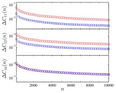
Figure 1: Mean relative deviation $\Delta C_{\alpha\beta}$ after averaging over $n$ independent configurations in the $NVT$ (blue squares) and $NPT$ ensemble (red circles) for pressure $P=0$ [$N=4000$, and $T=0.3$].

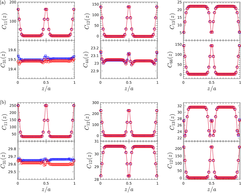
Figure 2: Simulated profiles of the nonzero local elastic constants in the $NVT$ (blue squares) and $NPT$ ensemble (red circles) at (a) $P=0$ and (b) $P=1.4$ [$N=4000$, $T=0.3$]. The lattice constants of the cubic unit cells are $a=1.6241$ for $P=0$ and $a=1.6016$ for $P=1.4$.

To compare the convergence behavior of the stress-stress FF in the two ensembles, we analyze the mean relative deviation of the bulk elastic constants with respect to their converged values in dependence of the number $n$ of configuration samples used for the ensemble averaging. This mean relative deviation was determined as follows. After averaging over $n$ equilibrated configurations (separated by 20 Monte Carlo steps) in one simulation run $i$, one obtains a value $C_{\alpha\beta}^{(i)}(n)$. This exhibits a relative deviation $|C_{\alpha\beta}^{(i)}(n)-C^{\textrm{ref}}_{\alpha\beta}|/C^{\textrm{ref}}_{\alpha\beta}$, where $C^{\textrm{ref}}_{\alpha\beta}$ refers to the converged value given in Table 1. The mean relative deviation $\Delta C_{\alpha\beta}(n)$ is obtained from averaging over a number $m=500$ of independent simulation runs $i=1,\ldots,m$, i. e. $\Delta C_{\alpha\beta}(n)=(\sum_{i=1}^{m}|C_{\alpha\beta}^{(i)}(n)-C^{\textrm{ref}}_{\alpha\beta}|/C^{\textrm{ref}}_{\alpha\beta})/m$. As can be seen from Fig. 1, the rate of convergence in both ensembles, i. e. the decrease of $\Delta C_{\alpha\beta}(n)$ with $n$, shows similar behavior. In the case of $C_{44}$, the mean relative deviations are almost the same for the two ensembles, and in the case of $C_{11}$ and $C_{12}$, they are by a factor of about two larger for the $NPT$ ensemble. After averaging over $n=10^{4}$ samples, the mean relative deviation is of the order 1% in both the $NVT$ and $NPT$ ensemble for $C_{11}$ and $C_{12}$, and about an order of magnitude smaller for $C_{44}$.

Finally, we compare the variation of the local elastic constants along one principal axis of the cubic unit cell in the two ensembles. To this end, we partition the simulation box into 500 thin slabs of equal thickness in the $z$-direction, that means 50 slabs per length of the cubic unit cell and calculate the local elastic constants for each slab. In the $NPT$ ensemble, where the size of the simulation box fluctuates, the slab thickness is always adjusted accordingly. Additionally, we average over the periodicity of the crystal, which here means that we perform an average over the elastic constants of every 50th slab. Generally, one should be careful with the physical interpretation of fields of elastic constants on spatial scales comparable to atomic distances, see the analysis and discussions in Yoshimoto et al. (2004); Barrat (2006); Tsamados et al. (2009); Molnàr et al. (2016). For the nearest-neighbor Lennard-Jones fcc crystal, however, it has been shown before VanWorkum and de Pablo (2003) that the elastic constants still relate stresses and strains linearly according to Hooke’s law even on such small scales.

Symmetry considerations for this arrangements predict that in total 12 local elastic constants are nonzero, where six of them are independent. For the partitioning in $z$-direction, these nonzero constants are $C_{11}(z)=C_{22}(z)$, $C_{12}(z)=C_{21}(z)$, $C_{13}(z)=C_{23}(z)$, $C_{31}(z)=C_{32}(z)$, $C_{33}(z)$, $C_{44}(z)=C_{55}(z)$, and $C_{66}(z)$. The results from the simulations confirm these predictions for both ensembles.

Figure 2 shows the profiles of the nonzero elastic constants $C_{\alpha\beta}(z)$ in the $NVT$ (blue squares) and the $NPT$ ensemble (red circles) for (a) $P=0.0$ and (b) $P=1.4$. For all elastic constants there is excellent agreement of the simulated data in the two ensembles. Due to the crystal symmetry, the profiles are symmetric with respect to the center of the cubic unit cell with lattice constant $a$, i. e. $C_{\alpha\beta}(z-a/2)=C_{\alpha\beta}(-z-a/2)$. We furthermore checked that an integration over the profiles gives bulk values, which exhibit the symmetries of the matrix in Eq. (18) and agree with the values listed in Table 1. As for the bulk values, the local elastic constants are larger for the higher pressure. The profiles $C_{13}(z)$ and $C_{44}(z)$ change their shape with the pressure change, where $C_{13}(z)$ shows an additional local maximum at $z=a/2$ at the higher pressure, and $C_{44}(z)$ exhibits a shallow local maximum at $z=a/2$ for $P=0$ and a local minimum at $P=1.4$.

V Application to a lipid bilayer model

As an example for the application of the stress-stress FF in the $NPT$ ensemble, we calculate the elastic constants for a simple coarse-grained model of a lipid bilayer as developed by Lenz and Schmid (LS model) Lenz and Schmid (2005, 2007); Lenz (2007). This model is a coarse-grained representation of single-tail amphiphilic molecules, where the hydrophilic part is represented by one head bead and the long aliphatic tail by six tails beads. Adjacent beads in one molecule are connected by finitely extensible nonlinear elastic (FENE) springs Grest and Kremer (1986) with potential

$$V_{\scriptscriptstyle\rm FENE}(r)=-\frac{v_{\scriptscriptstyle\rm FENE}}{2}(\Delta r_{\textrm{m}})^{2}\log\left[1-\left(\frac{r-r_{0}}{\Delta r_{\textrm{m}}}\right)^{2}\right]\,,$$ (19)

where $v_{\scriptscriptstyle\rm FENE}$ specifies the strength of the springs and $r$ the bead distance; $r_{0}$ is the bond length for the unstretched spring and $\Delta r_{\textrm{m}}$ is the maximal stretching distance. Three adjacent beads of a molecule with bond angle $\theta$ interact via the bond-angle potential

$$V_{\rm ba}(\theta)=v_{\rm ba}\left(1-\cos\theta\right)\,,$$ (20)

where $v_{\rm ba}$ regulates the stiffness of the chain molecules. Both the non-bonded beads belonging to the same molecule and the beads belonging to different molecules interact via a truncated Lennard-Jones potential

$$V_{\rm sc}(r) =\left[V_{\scriptscriptstyle\rm LJ}(r)-V_{\scriptscriptstyle\rm\rm LJ}(r_{\textrm{c}})\right]H(r_{\textrm{c}}-r)\,,$$ (21a)

$$V_{\scriptscriptstyle\rm LJ}(r) =v_{\scriptscriptstyle\rm LJ}\left[\left(\frac{\sigma_{\rm\scriptscriptstyle LJ}}{r}\right)^{12}-2\left(\frac{\sigma_{\rm\scriptscriptstyle LJ}}{r}\right)^{6}\right]\,,$$ (21b)

where $H(.)$ is the Heaviside step function [$H(x)=1$ for $x>0$ and zero otherwise]. The parameter $v_{\scriptscriptstyle\rm LJ}$ is the same for all types of the interacting beads and used as the energy unit. The $\sigma_{\rm\scriptscriptstyle LJ}$ are different for different types of beads, see Table 2. The length unit is set by $\sigma_{\rm\scriptscriptstyle LJ}$ for the tail-tail bead interactions. These units correspond to $v_{\scriptscriptstyle\rm LJ}\simeq 0.36\times 10^{-20}$ J and $\sigma_{\scriptscriptstyle\rm LJ}\simeq 6$ Å Lenz and Schmid (2005); Lenz (2007). The cutoff parameters $r_{\textrm{c}}$ correspond to the minimum of $V_{\scriptscriptstyle\rm LJ}(r)$ for head-head and head-tail bead interactions (i. e., $r_{\textrm{c}}=\sigma_{\scriptscriptstyle\rm LJ}$ in that case), leading to a purely repulsive interaction between these types of beads. For the tail-tail bead interactions, $r_{\textrm{c}}$ has a larger value, giving an attractive pair interaction for $\sigma_{\scriptscriptstyle\rm LJ}<r<r_{\textrm{c}}$. This attractive part facilitates a self-organization of the chain molecules into a double-layer structure.

To stabilize a lipid bilayer structure, the bead-spring chains representing the molecules are brought into contact with a solvent, which is also represented by simple beads. These interact with all lipid beads via $V_{\rm sc}(r)$ with parameters given in Table 2 (solely repulsive interactions), but they do not interact with themselves. All parameters of the LS model are summarized in Table 2. Units of temperature and pressure (as well as the elastic constants) are $v_{\scriptscriptstyle\rm LJ}/k_{\rm\scriptscriptstyle B}$ and $v_{\scriptscriptstyle\rm LJ}/\sigma_{\scriptscriptstyle\rm LJ}^{3}$, with $\sigma_{\scriptscriptstyle\rm LJ}$ for tail-tail bead interactions. As mentioned above in Sec. II, the truncation of the Lennard-Jones at the radii $r_{\textrm{c}}$ in Table 2 gives rise to discontinuities in the second-order derivatives of the respective potential and accordingly $\delta$-function contributions in the Born term, see Eqs. (7) and (12c). The corresponding impulsive contributions were taken into account for bead with pair distances $r$ in an interval $[r_{\textrm{c}}-\Delta r/2,r_{\textrm{c}}+\Delta r/2]$ with $\Delta r=0.02$ .

Table 2: Parameters of the interaction potentials in Eqs. (19)-(21) Lenz (2007), in units of the Lennard-Jones parameters $v_{\scriptscriptstyle\rm LJ}=1$ and $\sigma_{\scriptscriptstyle\rm LJ}=1$ for the tail-tail interactions.

interaction type	potential	parameters
tail-tail		$v_{\scriptscriptstyle\rm LJ}=1$, $\sigma_{\scriptscriptstyle\rm LJ}=1$, $r_{\textrm{c}}=2$
head-tail
solvent-tail	$V_{\rm sc}$	$v_{\scriptscriptstyle\rm LJ}=1$, $\sigma_{\scriptscriptstyle\rm LJ}=1.05$, $r_{\textrm{c}}=1.05$
head-head
solvent-head		$v_{\scriptscriptstyle\rm LJ}=1$, $\sigma_{\scriptscriptstyle\rm LJ}=1.1$, $r_{\textrm{c}}=1.1$
solvent-solvent	none
bond length	$V_{\scriptscriptstyle\rm FENE}$	$v_{\scriptscriptstyle\rm FENE}=100$, $r_{0}=0.7$, $\Delta r_{m}=0.2$
bond angle	$V_{\rm ba}$	$v_{\rm ba}=4.7$

Monte-Carlo simulations were performed as described in Lenz and Schmid (2005); Lenz (2007) under constant temperature $T=1.3$ and pressure $P=2$ for lipid bilayers with upper and lower leaflets consisting of $N=10\times 10$ lipid molecules; 7692 solvent beads were chosen for the solvent model. The lipid bilayer is oriented in the $xy$-plane and the center of mass of the lipid beads defines the origin of the coordinate system.

A representative example of an equilibrated configuration of the system with lipid bilayer and solvent beads is shown in Fig. 3. Because of the rotational symmetry around the $z$-axis, the elastic constants of the full lipid bilayer should exhibit transverse symmetry, corresponding to the block diagonal form

$$\begin{bmatrix}C_{11}&C_{12}&C_{13}&0&0&0\\ C_{12}&C_{11}&C_{13}&0&0&0\\ C_{13}&C_{13}&C_{33}&0&0&0\\ 0&0&0&C_{44}&0&0\\ 0&0&0&0&C_{44}&0\\ 0&0&0&0&0&C_{66}\end{bmatrix}$$ (22)

of the tensor in Voigt notation.

To determine the $C_{\alpha\beta}$ of the full lipid bilayer, we can now take advantage of the access to local elastic constants, which allows us to selectively average them over the region of the bilayer. Technically, we calculate the local constants with respect to the $z$-coordinate using Eqs. (12) by dividing the simulation box in 100 slabs with respect to the (instantaneous) box length in $z$-direction, i. e., we use the same method as described above in Sec. IV. The average slab thickness was $\Delta z=0.47$. The three-body contributions to the stress tensor and the Born-term resulting from the bond-angle potential in Eq. (20) are decomposed into pairwise contributions according to VanWorkum et al. (2006). In Eq. (12d) we take the ideal gas value $K=\rho_{\textrm{s}}k_{\rm\scriptscriptstyle B}T=P$, with $\rho_{\textrm{s}}$ the constant density of the solvent beads far from the lipid bilayer, see Fig. 4(a) .

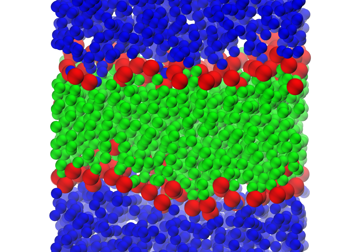
Figure 3: Snapshot of an equilibrated particle configuration of a lipid bilayer in the fluid phase together with the surrounding solvent from Monte-Carlo simulations of the LS model. Solvent beads are colored in blue, head beads in red, and tail beads in green.

Examples of the resulting profiles $C_{\alpha\beta}(z)$ are shown in Fig. 4(b)-(d), together with the density profiles of the head beads (dashed line), tail beads (solid line), and solvent beads (dotted line) in Fig. 4(a). The two profiles in Figs. 4(b) and (c) are representative of $C_{\alpha\beta}$ belonging to the first block diagonal element of (22) [$\alpha,\beta\in\{1,2,3\}$]: They are positive in the tail bead region and show an oscillation near the lipid-solvent interface, where the head beads have noticeable density, see Fig. 4(a). Near the interface a small $z$-interval exists, where $C_{11}$ and $C_{12}$ become negative. The profile in Fig. 4(d) is representative of the nonzero $C_{\alpha\beta}$ belonging to the second block diagonal element of (22) [$\alpha=\beta\in\{4,5,6\}$]. Here the impact of the head beads at the lipid-solvent interface is much less pronounced. All profiles in Figs. 4(b)-(d) exhibit a small dip close to the midplane of the bilayer at $z=0$ (”leaflet-interface”) and reflect well the spatial symmetry with respect to this midplane.

In the present case, the zero elements in (22) should give zero values also on the local scale. Indeed, we found the profiles calculated from the simulations to fluctuate around zero with a standard deviation of 0.42. In the solvent region, all profiles in Figs. 4(b)-(d) are flat with value $k_{\rm\scriptscriptstyle B}T\rho(z)=K=P=2$ for the $C_{\alpha\beta}(z)$, $1\leq\alpha,\beta\leq 3$, and zero value for the other $C_{\alpha\beta}(z)$. This is the expected behavior for the mutually non-interacting solvent beads, which correspond to an ideal gas. Since we are interested in the elastic constants of the full lipid bilayer, we are not investigating further here, on which spatial scale the profiles in Figs. 4(b)-(d) reflect a linear relation between local stresses and strains according to Hooke’s law.

By a spatial averaging over the profiles $C_{\alpha\beta}(z)$ the elastic constants of the full lipid bilayer are obtained,

$$C^{\scriptscriptstyle\textrm{LB}}_{\alpha\beta}=\frac{1}{(d_{+}-d_{-})}\int_{d_{-}}^{d_{+}}\mathrm{d}z\,C_{\alpha\beta}(z)\,,$$ (23)

where $d_{\pm}=z_{\pm}\pm\sigma_{\scriptscriptstyle\rm LJ}$ with $\sigma_{\scriptscriptstyle\rm LJ}$ the value for head-solvent interactions (see Table 2), and $z_{-}$ and $z_{+}$ are the average $z$-coordinates of the head bead in the lower and upper leaflet, respectively. By shifting these position with $\sigma_{\scriptscriptstyle\rm LJ}$ we take into account the soft core interaction range between head and solvent beads. The positions $d_{-}=-4.33$ and $d_{+}=4.30$ are marked by the vertical lines in Figs. 4(a)-(d). As can be seen from Fig. 4(a), they represent well the lower and upper limit of the bilayer. In Figs. 4(b)-(d) we see that they mark also the points, where the profiles of the local elastic constants cross over to the flat solvent regime.

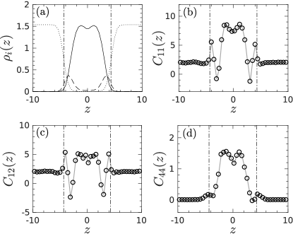
Figure 4: (a) Density profiles $\rho(z)$ of head beads (dashed line), tail beads (solid line) and solvent beads (dotted line). (b)-(d) Representative profiles $C_{\alpha\beta}(z)$ of elastic constants. The vertical lines mark the boundaries of the lipid bilayer region [see text and Eq. (23)]. Results were obtained from Monte-Carlo simulations at $T=1.3$ and $P=2$.

The tensor of elastic constants of the full lipid bilayer obtained from Eq. (23) is

$$C^{\scriptscriptstyle\textrm{LB}}\!=\!\left[\begin{array}[]{rrrrrr}5.11&3.00&2.80&-0.14&-0.22&-0.02\\ 3.03&5.34&3.08&-0.04&0.01&-0.03\\ 2.67&2.94&4.15&-0.06&-0.34&0.02\\ -0.15&-0.04&-0.05&0.91&0.02&-0.02\\ -0.21&0.01&-0.33&0.02&0.70&-0.04\\ -0.03&-0.03&0.03&-0.03&-0.04&1.18\end{array}\right]\,.$$ (24)

We see that the large elements are the $C_{\alpha\beta}$ with $1\leq\alpha,\beta\leq 3$, while values an order of magnitude smaller are obtained for those matrix elements, which should be zero according to the expected form in (22). From these elements we can estimate that the numerical uncertainty is about $\pm 0.3$. In terms of this numerical uncertainty, the diagonal elements $C_{44}$ and $C_{66}$, despite being small, have significant values, and the structure of (24) agrees with the expected symmetry of (22).

VI Conclusions

We derived a new stress-stress FF to calculate the tensors of bulk and local elastic constants in the $NPT$ ensemble based on formerly derived expressions for the $NVT$ ensemble and transformation rules for correlation functions between different ensembles. This FF allows the determination of elastic constants from simulations in the $NPT$ ensemble. We validated the FF for the nearest-neighbor Lennard-Jones solid and showed the agreement of the results with those obtained from corresponding simulations in the $NVT$ ensemble. As an application, we calculated the tensor of elastic constants for a simulated lipid bilayer in the fluid phase.

For solid materials, the new FF for the $NPT$ ensemble can facilitate the analysis of the pressure dependence of elastic constants. An efficient procedure to calculate elastic constants in the $NPT$ ensemble should in particular be useful for systems, which naturally need to be held under an external pressure. These are often soft matter structures forming in aqueous environments and exhibiting an elastic response behavior for small deformations, for example, lipid membranes or cell organelles. The access to local elastic constants provides a means for detailed analyses of heterogeneous systems, for which the studied lipid bilayer gives an example. As was shown recently, it is possible also to extend the methodology for studying time-dependent relaxation behavior of elastic moduli Wittmer et al. (2015).

Other interesting systems are structured composite materials, as, for example, sandwich materials with layer structure. A typical approach to calculate the elastic properties of such composite is to perform a weighted average over elastic properties of a homogeneous material assigned to each layer. Below a certain layer thickness, where the properties inside a layer become strongly influenced by interfacial effects, such calculation based on a simple layer representation will break down and the FF could then be used. From the theoretical point of view, one can study such composite systems with particle-based models and systematically analyze how large the substructures must be that a calculation based on a simple substructure representation becomes valid. Here it would be interesting to see whether one can find simple approximate rules, e. g. with respect to the influence of the particle interaction range.

Self-organized structures are often formed by complex molecules with interactions involving many-body forces, and these occur also for atomic systems when using accurate effective potentials derived from first-principle calculations. In the bulk, the stress-stress FF in the $NVT$ ensemble can be formulated for arbitrary many-body forces Lutsko (1989) and based on this, it is possible to take over the formulas in the $NPT$ ensemble as described. However, in the presence of many-body forces, it becomes more difficult to define a local stress tensor and associated stress-stress FF for local elastic constants. In some cases, as, e. g., for the bond-angle potential in Eq. (20), it is possible to decompose many-body forces into pair forces Vanegas et al. (2014); Torres-Sánchez et al. (2015); VanWorkum et al. (2006). For the general case, it would be desirable to investigate in more detail how many-body forces can be effectively handled in the determination of elastic constants.

References

- Ray (1988) J. R. Ray, Comput. Phys. Rep. 8, 109 (1988).
- Barrat (2006) J.-L. Barrat, in Computer Simulations in Condensed Matter Systems: From Materials to Chemical Biology Volume 2, Lecture Notes in Physics, Vol. 704 (Springer Berlin Heidelberg, 2006) pp. 287–307.
- Mizuno et al. (2013) H. Mizuno, S. Mossa, and J. L. Barrat, Phys. Rev. E 87, 042306 (2013).
- Meier (1993) R. J. Meier, Macromolecules 26, 4376 (1993).
- Aubouy et al. (2003) M. Aubouy, Y. Jiang, J. A. Glazier, and F. Graner, Granular Matter 5, 67 (2003).
- VanWorkum and de Pablo (2003) K. VanWorkum and J. J. de Pablo, Phys. Rev. E 67, 031601 (2003).
- Kluge et al. (1990) M. D. Kluge, D. Wolf, J. F. Lutsko, and S. R. Phillpot, J. Appl. Phys. 67, 2370 (1990).
- Griebel and Hamaekers (2004) M. Griebel and J. Hamaekers, Comput. Meth. Appl. Mech. Eng. 193, 1773 (2004).
- Parrinello and Rahman (1982) M. Parrinello and A. Rahman, J. Chem. Phys. 76, 2662 (1982).
- West et al. (2009) B. West, F. L. Brown, and F. Schmid, Biophys. J. 96, 101 (2009).
- Neder et al. (2010) J. Neder, B. West, P. Nielaba, and F. Schmid, J. Chem. Phys. 132, 115101 (2010).
- Ganguly et al. (2013) S. Ganguly, S. Sengupta, P. Sollich, and M. Rao, Phys. Rev. E 87, 042801 (2013).
- Gusev et al. (1996) A. A. Gusev, M. M. Zehnder, and U. W. Suter, Phys. Rev. B 54, 1 (1996).
- Lutsko (1988) J. F. Lutsko, J. Appl. Phys. 64, 1152 (1988).
- Lenz and Schmid (2007) O. Lenz and F. Schmid, Phys. Rev. Lett. 98, 058104 (2007).
- Parrinello and Rahman (1981) M. Parrinello and A. Rahman, J. Appl. Phys. 52, 7182 (1981).
- Ray and Rahman (1984) J. R. Ray and A. Rahman, J. Chem. Phys. 80, 4423 (1984).
- Lutsko (1989) J. F. Lutsko, J. Appl. Phys. 65, 2991 (1989).
- Xu et al. (2012) H. Xu, J. P. Wittmer, P. Polińska, and J. Baschnagel, Phys. Rev. E 86, 046705 (2012).
- Irving and Kirkwood (1950) J. H. Irving and J. G. Kirkwood, J. Chem. Phys. 18, 817 (1950).
- Yoshimoto et al. (2004) K. Yoshimoto, T. S. Jain, K. VanWorkum, P. F. Nealey, and J. J. de Pablo, Phys. Rev. Lett. 93, 175501 (2004).
- Kanigel et al. (2001) A. Kanigel, J. Adler, and E. Polturak, Int. J. Mod. Phys. C 12, 727 (2001).
- Yoshimoto et al. (2005) K. Yoshimoto, G. J. Papakonstantopoulos, J. F. Lutsko, and J. J. de Pablo, Phys. Rev. B 71, 184108 (2005).
- Gao et al. (2006) G. Gao, K. VanWorkum, J. D. Schall, and J. A. Harrison, J. Phys.: Condens. Mat. 18, 1737 (2006).
- Jun et al. (2007) C. Jun, C. Dong-Quan, and Z. Jing-Lin, Chin. Phys. 16, 2779 (2007).
- Wittmer et al. (2013a) J. P. Wittmer, H. Xu, P. Polińska, F. Weysser, and J. Baschnagel, J. Chem. Phys. 138, 12A533 (2013a).
- Wittmer et al. (2013b) J. P. Wittmer, H. Xu, P. Polińska, C. Gillig, J. Helfferich, F. Weysser, and J. Baschnagel, Eur. Phys. J. E 36, 131 (2013b).
- Wittmer et al. (2013c) J. P. Wittmer, H. Xu, P. Polińska, F. Weysser, and J. Baschnagel, J. Chem. Phys. 138, 191101 (2013c).
- Note (1) The pair potential should decrease faster than with the particle distance , or, for slower decaying pair potentials, screening effects should lead to an effective decay faster than .
- Lebowitz et al. (1967) J. L. Lebowitz, J. K. Percus, and L. Verlet, Phys. Rev. 153, 250 (1967).
- Note (2) This formula has the following meaning: In the ensemble the average pressure has the value , and it is this pressure that defines the ensemble for evaluating the average. The partial derivatives with respect to refer to changes of the corresponding quantities in the ensemble with , and need to be evaluated at the pressure .
- Barron and Klein (1965) T. H. K. Barron and M. L. Klein, Proc. Phys. Soc. 85, 523 (1965).
- Voigt (1910) W. Voigt, Lehrbuch der Kristallphysik (Teubner, Leipzig, 1910).
- Cowley (1983) E. R. Cowley, Phys. Rev. B 28, 3160 (1983).
- Sprik et al. (1984) M. Sprik, R. W. Impey, and M. L. Klein, Phys. Rev. B 29, 4368 (1984).
- Ray et al. (1985) J. R. Ray, M. C. Moody, and A. Rahman, Phys. Rev. B 32, 733 (1985).
- Landau and Binder (2014) D. P. Landau and K. Binder, A Guide to Monte Carlo Simulations in Statistical Physics, 4th ed. (Cambridge University Press, 2014).
- Nye (1985) J. F. Nye, Physical Properties of Crystals (Oxford University Press, 1985).
- Tsamados et al. (2009) M. Tsamados, A. Tanguy, C. Goldenberg, and J.-L. Barrat, Phys. Rev. E 80, 026112 (2009).
- Molnàr et al. (2016) G. Molnàr, P. Ganster, J. Török, and A. Tanguy, J. Non-Cryst. Solids 440, 12 (2016).
- Lenz and Schmid (2005) O. Lenz and F. Schmid, J. Mol. Liquids 117, 147 (2005).
- Lenz (2007) O. Lenz, Computer simulation of lipid bilayers, Ph.D. thesis, Universität Bielefeld, https://pub.uni-bielefeld.de/download/2301947/2301950 (2007).
- Grest and Kremer (1986) G. S. Grest and K. Kremer, Phys. Rev. A. 33, 3628 (1986).
- Note (3) A more sophisticated method for treating the impulsive contributions is given in Xu et al. (2012).
- VanWorkum et al. (2006) K. VanWorkum, G. Gao, J. D. Schall, and J. A. Harrison, J. Chem. Phys. 125, 114506 (2006).
- Note (4) In the thermodynamic limit, the lipid beads would occupy a zero fraction of the total volume, yielding a bulk modulus for the whole system. For a small system, the bulk modulus shows deviations from its thermodynamic limit due to contributions from the lipid bilayer.
- Wittmer et al. (2015) J. P. Wittmer, H. Xu, and J. Baschnagel, Phys. Rev. E 91, 022107 (2015).
- Vanegas et al. (2014) J. M. Vanegas, A. Torres-Sanchez, and M. Arroyo, J. Chem. Theory Comput. 10, 691 (2014).
- Torres-Sánchez et al. (2015) A. Torres-Sánchez, J. M. Vanegas, and M. Arroyo, Phys. Rev. Lett. 114, 258102 (2015).