1000 \NewEnvironproofatend+=
\pat@proofof \pat@label.
∎
Fast Policy Learning through Imitation and Reinforcement
Abstract
Imitation learning (IL) consists of a set of tools that leverage expert demonstrations to quickly learn policies. However, if the expert is suboptimal, IL can yield policies with inferior performance compared to reinforcement learning (RL). In this paper, we aim to provide an algorithm that combines the best aspects of RL and IL. We accomplish this by formulating several popular RL and IL algorithms in a common mirror descent framework, showing that these algorithms can be viewed as a variation on a single approach. We then propose loki, a strategy for policy learning that first performs a small but random number of IL iterations before switching to a policy gradient RL method. We show that if the switching time is properly randomized, loki can learn to outperform a suboptimal expert and converge faster than running policy gradient from scratch. Finally, we evaluate the performance of loki experimentally in several simulated environments.
1 INTRODUCTION
Reinforcement learning (RL) has emerged as a promising technique to tackle complex sequential decision problems. When empowered with deep neural networks, RL has demonstrated impressive performance in a range of synthetic domains (Mnih et al.,, 2013; Silver et al.,, 2017). However, one of the major drawbacks of RL is the enormous number of interactions required to learn a policy. This can lead to prohibitive cost and slow convergence when applied to real-world problems, such as those found in robotics (Pan et al.,, 2017).
Imitation learning (IL) has been proposed as an alternate strategy for faster policy learning that works by leveraging additional information provided through expert demonstrations (Pomerleau,, 1989; Schaal,, 1999). However, despite significant recent breakthroughs in our understanding of imitation learning (Ross et al.,, 2011; Cheng and Boots,, 2018), the performance of IL is still highly dependent on the quality of the expert policy. When only a suboptimal expert is available, policies learned with standard IL can be inferior to the policies learned by tackling the RL problem directly with approaches such as policy gradients.
Several recent attempts have endeavored to combine RL and IL (Ross and Bagnell,, 2014; Chang et al.,, 2015; Nair et al.,, 2017; Rajeswaran et al.,, 2017; Sun et al.,, 2018). These approaches incorporate the cost information of the RL problem into the imitation process, so the learned policy can both improve faster than their RL-counterparts and outperform the suboptimal expert policy. Despite reports of improved empirical performance, the theoretical understanding of these combined algorithms are still fairly limited (Rajeswaran et al.,, 2017; Sun et al.,, 2018). Furthermore, some of these algorithms have requirements that can be difficult to satisfy in practice, such as state resetting (Ross and Bagnell,, 2014; Chang et al.,, 2015).
In this paper, we aim to provide an algorithm that combines the best aspects of RL and IL. We accomplish this by first formulating first-order RL and IL algorithms in a common mirror descent framework, and show that these algorithms can be viewed as a single approach that only differs in the choice of first-order oracle. On the basis of this new insight, we address the difficulty of combining IL and RL with a simple, randomized algorithm, named loki (Locally Optimal search after -step Imitation). As its name suggests, loki operates in two phases: picking randomly, it first performs steps of online IL and then improves the policy with a policy gradient method afterwards. Compared with previous methods that aim to combine RL and IL, loki is extremely straightforward to implement. Furthermore, it has stronger theoretical guarantees: by properly randomizing , loki performs as if directly running policy gradient steps with the expert policy as the initial condition. Thus, not only can loki improve faster than common RL methods, but it can also significantly outperform a suboptimal expert. This is in contrast to previous methods, such as AggreVatTe (Ross and Bagnell,, 2014), which generally cannot learn a policy that is better than a one-step improvement over the expert policy. In addition to these theoretical contributions, we validate the performance of loki in multiple simulated environments. The empirical results corroborate our theoretical findings.
2 PROBLEM DEFINITION
We consider solving discrete-time -discounted infinite-horizon RL problems.111loki can be easily adapted to finite-horizon problems. Let and be the state and the action spaces, and let be the policy class. The objective is to find a policy that minimizes an accumulated cost defined as
| (1) |
in which , , is the instantaneous cost, and denotes the distribution of trajectories generated by running the stationary policy starting from .
We denote as the Q-function under policy and as the associated value function, where denotes the action distribution given state . In addition, we denote as the state distribution at time generated by running the policy for the first steps, and we define a joint distribution which has support . Note that, while we use the notation , the policy class can be either deterministic or stochastic.
We generally will not deal with the objective function in (1) directly. Instead, we consider a surrogate problem
| (2) |
where is the (dis)advantage function with respect to some fixed reference policy . For compactness of writing, we will often omit the random variable in expectation; e.g., the objective function in (2) will be written as for the remainder of paper.
By the performance difference lemma below (Kakade and Langford,, 2002), it is easy to see that solving (2) is equivalent to solving (1).
Lemma 1.
(Kakade and Langford,, 2002) Let and be two policies and be the (dis)advantage function with respect to running . Then it holds that
| (3) |
3 FIRST-ORDER RL AND IL
We formulate both first-order RL and IL methods within a single mirror descent framework (Nemirovski et al.,, 2009), which includes common update rules (Sutton et al.,, 2000; Kakade,, 2002; Peters and Schaal,, 2008; Peters et al.,, 2010; Rawlik et al.,, 2012; Silver et al.,, 2014; Schulman et al., 2015b, ; Ross et al.,, 2011; Sun et al.,, 2017). We show that policy updates based on RL and IL mainly differ in first-order stochastic oracles used, as summarized in Table 1.
| Method | First-Order Oracle |
|---|---|
| policy gradient (Section 3.2.1) | |
| DAggereD (Section 3.2.2) | |
| AggreVaTeD (Section 3.2.2) | |
| slols (Section 6) | |
| thor (Section 6) |
3.1 MIRROR DESCENT
We begin by defining the iterative rule to update policies. We assume that the learner’s policy is parametrized by some , where is a closed and convex set, and that the learner has access to a family of strictly convex functions .
To update the policy, in the th iteration, the learner receives a vector from a first-order oracle, picks , and then performs a mirror descent step:
| (4) |
where is a prox-map defined as
| (5) |
is the step size, and is the Bregman divergence associated with (Bregman,, 1967): .
By choosing proper , the mirror descent framework in (4) covers most RL and IL algorithms. Common choices of include negative entropy (Peters et al.,, 2010; Rawlik et al.,, 2012), (Sutton et al.,, 2000; Silver et al.,, 2014), and with as the Fisher information matrix (Kakade,, 2002; Peters and Schaal,, 2008; Schulman et al., 2015a, ).
3.2 FIRST-ORDER ORACLES
While both first-order RL and IL methods can be viewed as performing mirror descent, they differ in the choice of the first-order oracle that returns the update direction . Here we show the vector of both approaches can be derived as a stochastic approximation of the (partial) derivative of with respect to policy , but with a different reference policy .
3.2.1 Policy Gradients
A standard approach to RL is to treat (1) as a stochastic nonconvex optimization problem. In this case, in mirror descent (4) is an estimate of the policy gradient (Williams,, 1992; Sutton et al.,, 2000).
To compute the policy gradient in the th iteration, we set the current policy as the reference policy in (3) (i.e. ), which is treated as constant in in the following policy gradient computation. Because , using (3), the policy gradient can be written as222We assume the cost is sufficiently regular so that the order of differentiation and expectation can exchange.
| (6) |
The above expression is unique up to a change of baselines: is equivalent to , because , where is also called a control variate (Greensmith et al.,, 2004).
The exact formulation of depends on whether the policy is stochastic or deterministic. For stochastic policies,333A similar equation holds for reparametrization (Grathwohl et al.,, 2017). we can compute it with the likelihood-ratio method and write
| (7) |
For deterministic policies, we replace the expectation as evaluation (as it is the expectation over a Dirac delta function, i.e. ) and use the chain rule:
| (8) |
Substituting (7) or (8) back into (3.2.1), we get the equation for stochastic policy gradient (Sutton et al.,, 2000) or deterministic policy gradient (Silver et al.,, 2014). Note that the above equations require the exact knowledge, or an unbiased estimate, of . In practice, these terms are further approximated using function approximators, leading to biased gradient estimators (Konda and Tsitsiklis,, 2000; Schulman et al., 2015b, ; Mnih et al.,, 2016).
3.2.2 Imitation Gradients
An alternate strategy to RL is IL. In particular, we consider online IL, which interleaves data collection and policy updates to overcome the covariate shift problem of traditional batch IL (Ross et al.,, 2011). Online IL assumes that a (possibly suboptimal) expert policy is available as a black-box oracle, from which demonstrations can be queried for any given state . Due to this requirement, the expert policy in online IL is often an algorithm (rather than a human demonstrator), which is hard-coded or based on additional computational resources, such as trajectory optimization (Pan et al.,, 2017). The goal of IL is to learn a policy that can perform similar to, or better than, the expert policy.
Rather than solving the stochastic nonconvex optimization directly, online IL solves an online learning problem with per-round cost in the th iteration defined as
| (9) |
where is a surrogate loss satisfying the following condition: For all and , there exists a constant such that
| (10) |
By Lemma 1, this implies . Namely, in the th iteration, online IL attempts to minimize an online upper-bound of .
DAgger (Ross et al.,, 2011) chooses to be a strongly convex function that penalizes the difference between the learner’s policy and the expert’s policy, where is some metric of space (e.g., for a continuous action space Pan et al., (2017) choose ). More directly, AggreVatTe simply chooses (Ross and Bagnell,, 2014); in this case, the policy learned with online IL can potentially outperform the expert policy.
First-order online IL methods operate by updating policies with mirror descent (4) with as an estimate of
| (11) |
Similar to policy gradients, the implementation of (11) can be executed using either (7) or (8) (and with a control variate). One particular case of (11), with , is known as AggreVaTeD (Sun et al.,, 2017),
| (12) |
Similarly, we can turn DAgger into a first-order method, which we call DAggereD, by using as an estimate of the first-order oracle
| (13) |
A comparison is summarized in Table 1.
4 THEORETICAL COMPARISON
With the first-order oracles defined, we now compare the performance and properties of performing mirror descent with policy gradient or imitation gradient. We will see that while both approaches share the same update rule in (4), the generated policies have different behaviors: using policy gradient generates a monotonically improving policy sequence, whereas using imitation gradient generates a policy sequence that improves on average. Although the techniques used in this section are not completely new in the optimization literature, we specialize the results to compare performance and to motivate loki in the next section. The proofs of this section are included in Appendix B.
4.1 POLICY GRADIENTS
We analyze the performance of policy gradients with standard techniques from nonconvex analysis.
Proposition 1.
Let be -smooth and be -strongly convex with respect to norm . Assume . For , it satisfies
where the expectation is due to randomness of sampling , and . is a gradient surrogate.
Proposition 1 shows that monotonic improvement can be made under proper smoothness assumptions if the step size is small and noise is comparably small with the gradient size. However, the final policy’s performance is sensitive to the initial condition , which can be poor for a randomly initialized policy.
Proposition 1 also suggests that the size of the gradient does not converge to zero on average. Instead, it converges to a size proportional to the sampling noise of policy gradient estimates due to the linear dependency of on . This phenomenon is also mentioned by Ghadimi et al., (2016). We note that this pessimistic result is because the prox-map (5) is nonlinear in for general and . However, when is quadratic and is unconstrained, the convergence of to zero on average can be guaranteed (see Appendix B.1 for a discussion).
4.2 IMITATION GRADIENTS
While applying mirror descent with a policy gradient can generate a monotonically improving policy sequence, applying the same algorithm with an imitation gradient yields a different behavior. The result is summarized below, which is a restatement of (Ross and Bagnell,, 2014, Theorem 2.1), but is specialized for mirror descent.
Proposition 2.
Assume is -strongly convex with respect to .444A function is said to be -strongly convex with respect to on a set if for all , . Assume and almost surely. For with , it holds
where the expectation is due to randomness of sampling , and .
Proposition 2 is based on the assumption that is strongly convex, which can be verified for certain problems (Cheng and Boots,, 2018). Consequently, Proposition 2 shows that the performance of the policy sequence on average can converge close to the expert’s performance , with additional error that is proportional to and .
is an upper bound of the average regret, which is less than for a large enough step size.555The step size should be large enough to guarantee convergence, where denotes Big-O but omitting dependency. However, it should be bounded since . This characteristic is in contrast to policy gradient, which requires small enough step sizes to guarantee local improvement.
measures the expressiveness of the policy class . It can be negative if there is a policy in that outperforms the expert policy in terms of . However, since online IL attempts to minimize an online upper bound of the accumulated cost through a surrogate loss , the policy learned with imitation gradients in general cannot be better than performing one-step policy improvement from the expert policy (Ross and Bagnell,, 2014; Cheng and Boots,, 2018). Therefore, when the expert is suboptimal, the reduction from nonconvex optimization to online convex optimization can lead to suboptimal policies.
Finally, we note that updating policies with imitation gradients does not necessarily generate a monotonically improving policy sequence, even for deterministic problems; whether the policy improves monotonically is completely problem dependent (Cheng and Boots,, 2018). Without going into details, we can see this by comparing policy gradient in (3.2.1) and the special case of imitation gradient in (12). By Lemma 3, we see that
Therefore, even with , the negative of the direction in (12) is not necessarily a descent direction; namely applying (12) to update the policy is not guaranteed to improve the policy performance locally.
5 IMITATE-THEN-REINFORCE
To combine the benefits from RL and IL, we propose a simple randomized algorithm loki: first perform steps of mirror descent with imitation gradient and then switch to policy gradient for the rest of the steps. Despite the algorithm’s simplicity, we show that, when is appropriately randomized, running loki has similar performance to performing policy gradient steps directly from the expert policy.
5.1 ALGORITHM: loki
The algorithm loki is summarized in Algorithm 1. The algorithm is composed of two phases: an imitation phase and a reinforcement phase. In addition to learning rates, loki receives three hyperparameters (, , ) which determine the probability of random switching at time . As shown in the next section, these three hyperparameters can be selected fairly simply.
Imitation Phase
Before learning, loki first randomly samples a number according to the prescribed probability distribution (15). Then it performs steps of mirror descent with imitation gradient. In our implementation, we set
| (14) |
which is the KL-divergence between the two policies. It can be easily shown that a proper constant exists satisfying the requirement of in (10) (Gibbs and Su,, 2002). While using (14) does not guarantee learning a policy that outperforms the expert due to , with another reinforcement phase available, the imitation phase of loki is only designed to quickly bring the initial policy closer to the expert policy. Compared with choosing as in AggreVaTeD, one benefit of choosing (or its variants, e.g. ) is that it does not require learning a value function estimator. In addition, the imitation gradient can be calculated through reparametrization instead of a likelihood-ratio (Tucker et al.,, 2017), as now is presented as a differentiable function in . Consequently, the sampling variance of imitation gradient can be significantly reduced by using multiple samples of (with a single query from the expert policy) and then performing averaging.
Reinforcement Phase
After the imitation phase, loki switches to the reinforcement phase. At this point, the policy is much closer to the expert policy than the initial policy . In addition, an estimate of is also available. Because the learner’s policies were applied to collect data in the previous online imitation phase, can already be updated accordingly, for example, by minimizing TD error. Compared with other warm-start techniques, loki can learn both the policy and the advantage estimator in the imitation phase.
5.2 ANALYSIS
We now present the theoretical properties of loki. The analysis is composed of two steps. First, we show the performance of in Theorem 1, a generalization of Proposition 2 to consider the effects of non-uniform random sampling. Next, combining Theorem 1 and Proposition 1, we show the performance of loki in Theorem 2. The proofs are given in Appendix C.
Theorem 1.
Let , , and . Let be a discrete random variable such that
| (15) |
Suppose is -strongly convex with respect to , , and almost surely. Let be generated by running mirror descent with step size . For , it holds that
where the expectation is due to sampling and , , , , and
Suppose . Theorem 1 says that the performance of in expectation converges to in a rate of when a proper step size is selected. In addition to the convergence rate, we notice that the performance gap between and is bounded by . is a weighted version of the expressiveness measure of policy class in Proposition 2, which can be made small if is rich enough with respect to the suboptimal expert policy. measures the size of the decision space with respect to the class of regularization functions that the learner uses in mirror descent. The dependency on is because Theorem 1 performs a suffix random sampling with . While the presence of increases the gap, its influence can easily made small with a slightly large due to the factor .
In summary, due to the sublinear convergence rate of IL, does not need to be large (say less than 100) as long as ; on the other hand, due to the factor, is also small (say less than ) as long as it is large enough to cancel out the effects of . Finally, we note that, like Proposition 2, Theorem 1 encourages using larger step sizes, which can further boost the convergence of the policy in the imitation phase of loki.
Theorem 2.
Running loki holds that
where the expectation is due to sampling and .
Firstly, Theorem 2 shows that can perform better than the expect policy , and, in fact, it converges to a locally optimal policy on average under the same assumption as in Proposition 1. Compare with to running policy gradient steps directly from the expert policy, running loki introduces an additional gap . However, as discussed previously, and are reasonably small, for usual in RL. Therefore, performing loki almost has the same effect as using the expert policy as the initial condition, which is the best we can hope for when having access to an expert policy.
We can also compare loki with performing usual policy gradient updates from a randomly initialized policy. The performance difference can be easily shown as . Therefore, if performing steps of policy gradient from gives a policy with performance worse than , then loki is favorable.
6 RELATED WORK
We compare loki with some recent attempts to incorporate the loss information of RL into IL so that it can learn a policy that outperforms the expert policy. As discussed in Section 4, when , AggreVaTe(D) can potentially learn a policy that is better than the expert policy (Ross and Bagnell,, 2014; Sun et al.,, 2017). However, implementing AggreVaTe(D) exactly as suggested by theory can be difficult and inefficient in practice. On the one hand, while can be learned off-policy using samples collected by running the expert policy, usually the estimator quality is unsatisfactory due to covariate shift. On the other hand, if is learned on-policy, it requires restarting the system from any state, or requires performing -times more iterations to achieve the same convergence rate as other choices of such as in loki; both of which are impractical for usual RL problems.
Recently, Sun et al., (2018) proposed thor (Truncated HORizon policy search) which solves a truncated RL problem with the expert’s value function as the terminal loss to alleviate the strong dependency of AggreVaTeD on the quality of . Their algorithm uses an -step truncated advantage function defined as . While empirically the authors show that the learned policy can improve over the expert policy, the theoretical properties of thor remain somewhat unclear.666The algorithm actually implemented by Sun et al., (2018) does not solve precisely the same problem analyzed in theory. In addition, thor is more convoluted to implement and relies on multiple advantage function estimators. By contrast, loki has stronger theoretical guarantees, while being straightforward to implement with off-the-shelf learning algorithms.
Finally, we compare loki with lols (Locally Optimal Learning to Search), proposed by Chang et al., (2015). lols is an online IL algorithm which sets , where and is a mixed policy that at each time step chooses to run the current policy with probability and the expert policy with probability . Like AggreVaTeD, lols suffers from the impractical requirement of estimating , which relies on the state resetting assumption.
Here we show that such difficulty can be addressed by using the mirror descent framework with as an estimate of , where . That is, the first-order oracle is simply a convex combination of policy gradient and AggreVaTeD gradient. We call such linear combination slols (simple lols) and we show it has the same performance guarantee as lols.
Theorem 3.
Under the same assumption in Proposition 2, running slols generates a policy sequence, with randomness due to sampling , satisfying
where and .
In fact, the performance in Theorem 3 is actually a lower bound of Theorem 3 in (Chang et al.,, 2015).777The main difference is due to technicalities. In Chang et al., (2015), is compared with a time-varying policy. Theorem 3 says that on average has performance between the expert policy and the intermediate cost , as long as is small (i.e., there exists a single policy in that is better than the expert policy or the local improvement from any policy in ). However, due to the presence of , despite , it is not guaranteed that . As in Chang et al., (2015), either lols or slols can necessarily perform on average better than the expert policy . Finally, we note that recently both Nair et al., (2017) and Rajeswaran et al., (2017) propose a scheme similar to slols, but with the AggreVaTe(D) gradient computed using offline batch data collected by the expert policy. However, there is no theoretical analysis of this algorithm’s performance.
7 EXPERIMENTS
We evaluate loki on several robotic control tasks from OpenAI Gym (Brockman et al.,, 2016) with the DART physics engine (Lee et al.,, 2018)888The environments are defined in DartEnv, hosted at https://github.com/DartEnv. and compare it with several baselines: trpo (Schulman et al., 2015a, ), trpo from expert, DAggereD (the first-order version of DAgger (Ross et al.,, 2011) in (13)), slols (Section 6), and thor (Sun et al.,, 2018).
7.1 TASKS
We consider the following tasks. In all tasks, the discount factor of the RL problem is set to . The details of each task are specified in Table A in Appendix A.
Inverted Pendulum
This is a classic control problem, and its goal is to swing up an pendulum and to keep it balanced in a upright posture. The difficulty of this task is that the pendulum cannot be swung up directly due to a torque limit.
Locomotion
The goal of these tasks (Hopper, 2D Walker, and 3D Walker) is to control a walker to move forward as quickly as possible without falling down. In Hopper, the walker is a monoped, which is subjected to significant contact discontinuities, whereas the walkers in the other tasks are bipeds. In 2D Walker, the agent is constrained to a plane to simplify balancing.
Robot Manipulator
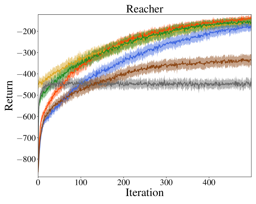
In the Reacher task, a 5-DOF (degrees-of-freedom) arm is controlled to reach a random target position in 3D space. The reward consists of the negative distance to the target point from the finger tip plus a control magnitude penalty. The actions correspond to the torques applied to the joints.
7.2 ALGORITHMS
We compare five algorithms (loki, trpo, DAggereD, thor, slols) and the idealistic setup of performing policy gradient steps directly from the expert policy (Ideal). To facilitate a fair comparison, all the algorithms are implemented based on a publicly available trpo implementation (Dhariwal et al.,, 2017). Furthermore, they share the same parameters except for those that are unique to each algorithm as listed in Table A in Appendix A. The experimental results averaged across random seeds are reported in Section 7.3.
Policy and Value Networks
Feed-forward neural networks are used to construct the policy networks and the value networks in all the tasks (both have two hidden layers and 32 tanh units per layer). We consider Gaussian stochastic policies, i.e. for any state , is Gaussian distributed. The mean of the Gaussian , as a function of state, is modeled by the policy network, and the covariance matrix of Gaussian is restricted to be diagonal and independent of state. The policy networks and the value function networks are initialized randomly, except for the ideal setup (trpo from expert), which is initialized as the expert.
Expert Policy
The same sub-optimal expert is used by all algorithms (loki, DAggereD, slols, and thor). It is obtained by running trpo and stopping it before convergence. The estimate of the expert value function (required by slols and thor) is learned by minimizing the sum of squared TD(0) error on a large separately collected set of demonstrations of this expert. The final explained variance for all the tasks is more than (see Appendix A).
First-Order Oracles
The on-policy advantage in the first-order oracles for trpo, slols, and loki (in the reinforcement phase) is implemented using an on-policy value function estimator and Generalized Advantage Estimator (GAE) (Schulman et al., 2015b, ). For DAggereD and the imitation phase of loki, the first-order oracle is calculated using (14). For slols, we use the estimate . And for thor, of the truncated-horizon problem is approximated by Monte-Carlo samples with an on-policy value function baseline estimated by regressing on these Monte-Carlo samples. Therefore, for all methods, an on-policy component is used in constructing the first-order oracle. The exponential weighting in GAE is ; the mixing coefficient in slols is ; in loki is reported in Table A in Appendix A, and , and .
Mirror Descent
After receiving an update direction from the first-order oracle, a KL-divergence-based trust region is specified. This is equivalent to setting the strictly convex function in mirror descent to and choosing a proper learning rate. In our experiments, a larger KL-divergence limit () is selected for imitation gradient (14) (in DAggereD and in the imitation phase of loki), and a smaller one () is set for all other algorithms. This decision follows the guideline provided by the theoretical analysis in Section 3.2.2 and is because of the low variance in calculating the gradient of (14). Empirically, we observe using the larger KL-divergence limit with policy gradient led to high variance and instability.
7.3 EXPERIMENTAL RESULTS
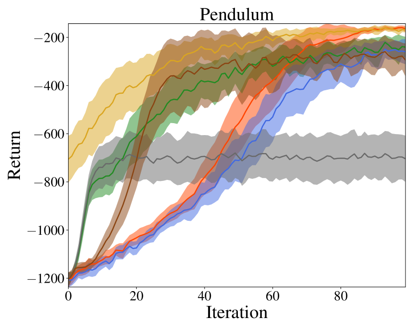
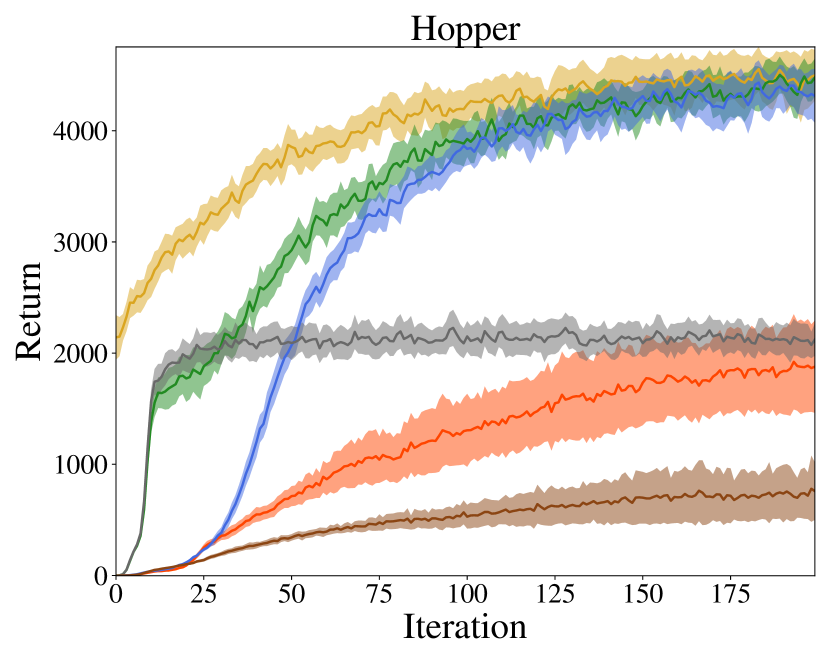
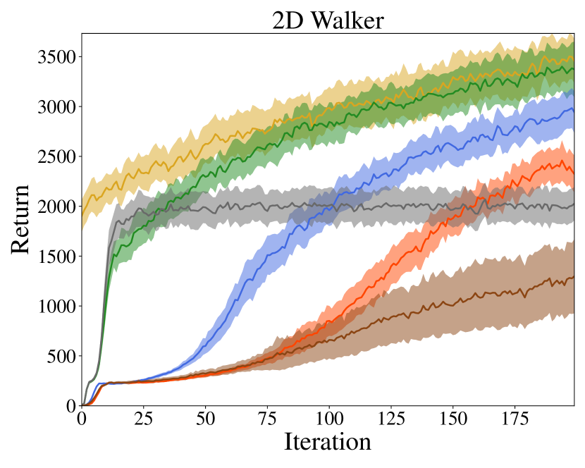
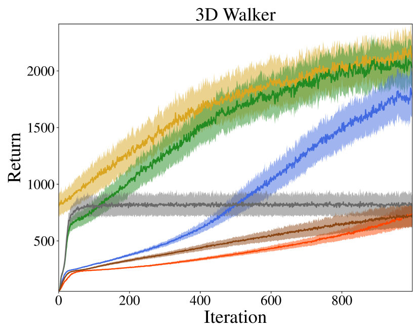
We report the performance of these algorithms on various tasks in Figure 1. The performance is measured by the accumulated rewards, which are directly provided by OpenAI Gym.
We first establish the performance of two baselines, which represent standard RL (trpo) and standard IL (DAggereD). trpo is able to achieve considerable and almost monotonic improvement from a randomly initialized policy. DAggereD reaches the performance of the suboptimal policy in a relatively very small number of iterations, e.g. 15 iterations in 2D Walker, in which the suboptimal policy to imitate is trpo at iteration 100. However, it fails to outperform the suboptimal expert.
Then, we evaluate the proposed algorithm loki and Ideal, the performance of which we wish to achieve in theory. loki consistently enjoys the best of both trpo and DAggereD: it improves as fast as DAggereD at the beginning, keeps improving, and then finally matches the performance of Ideal after transitioning into the reinforcement phase. Interestingly, the on-policy value function learned, though not used, in the imitation phase helps loki transition from imitation phase to reinforcement phase smoothly.
Lastly, we compare loki to the two other baselines (slols and thor) that combine RL and IL. loki outperforms these two baselines by a considerably large margin in Hopper, 2D Walker, and 3D Walker; but surprisingly, the performance of slols and thor are inferior even to trpo on these tasks. The main reason is that the first-order oracles of both methods is based on an estimated expert value function . As is only regressed on the data collected by running the expert policy, large covariate shift error could happen if the dimension of the state and action spaces are high, or if the uncontrolled system is complex or unstable. For example, in the low-dimensional Pendulum task and the simple Reacher task, the expert value function can generalize better. As a result, in these two cases, lols and thor achieve super-expert performance. However, in more complex tasks, where the effects of covariant shift amplifies exponentially with the dimension of the state space, thor and slols start to suffer from the inaccuracy of , as illustrated in the 2D Walker and 3D Walker tasks.
8 CONCLUSION
We present a simple, elegant algorithm, loki, that combines the best properties of RL and IL. Theoretically, we show that, by randomizing the switching time, loki can perform as if running policy gradient steps directly from the expert policy. Empirically, loki demonstrates superior performance compared with the expert policy and more complicated algorithms that attempt to combine RL and IL.
Acknowledgements
This work was supported in part by NSF NRI Award 1637758, NSF CAREER Award 1750483, and NSF Graduate Research Fellowship under Grant No. 2015207631.
References
- Bregman, (1967) Bregman, L. M. (1967). The relaxation method of finding the common point of convex sets and its application to the solution of problems in convex programming. USSR Computational Mathematics and Mathematical Physics, 7(3):200–217.
- Brockman et al., (2016) Brockman, G., Cheung, V., Pettersson, L., Schneider, J., Schulman, J., Tang, J., and Zaremba, W. (2016). Openai gym.
- Chang et al., (2015) Chang, K.-W., Krishnamurthy, A., Agarwal, A., Daume III, H., and Langford, J. (2015). Learning to search better than your teacher.
- Cheng and Boots, (2018) Cheng, C.-A. and Boots, B. (2018). Convergence of value aggregation for imitation learning. In International Conference on Artificial Intelligence and Statistics, pages 1801–1809.
- Dhariwal et al., (2017) Dhariwal, P., Hesse, C., Klimov, O., Nichol, A., Plappert, M., Radford, A., Schulman, J., Sidor, S., and Wu, Y. (2017). Openai baselines.
- Ghadimi et al., (2016) Ghadimi, S., Lan, G., and Zhang, H. (2016). Mini-batch stochastic approximation methods for nonconvex stochastic composite optimization. Mathematical Programming, 155(1-2):267–305.
- Gibbs and Su, (2002) Gibbs, A. L. and Su, F. E. (2002). On choosing and bounding probability metrics. International Statistical Review, 70(3):419–435.
- Grathwohl et al., (2017) Grathwohl, W., Choi, D., Wu, Y., Roeder, G., and Duvenaud, D. (2017). Backpropagation through the void: Optimizing control variates for black-box gradient estimation. arXiv preprint arXiv:1711.00123.
- Greensmith et al., (2004) Greensmith, E., Bartlett, P. L., and Baxter, J. (2004). Variance reduction techniques for gradient estimates in reinforcement learning. Journal of Machine Learning Research, 5(Nov):1471–1530.
- Juditsky et al., (2011) Juditsky, A., Nemirovski, A., et al. (2011). First order methods for nonsmooth convex large-scale optimization, i: general purpose methods. Optimization for Machine Learning, pages 121–148.
- Kakade and Langford, (2002) Kakade, S. and Langford, J. (2002). Approximately optimal approximate reinforcement learning. In International Conference on Machine Learning, volume 2, pages 267–274.
- Kakade, (2002) Kakade, S. M. (2002). A natural policy gradient. In Advances in Neural Information Processing Systems, pages 1531–1538.
- Konda and Tsitsiklis, (2000) Konda, V. R. and Tsitsiklis, J. N. (2000). Actor-critic algorithms. In Advances in Neural Information Processing Systems, pages 1008–1014.
- Lee et al., (2018) Lee, J., Grey, M. X., Ha, S., Kunz, T., Jain, S., Ye, Y., Srinivasa, S. S., Stilman, M., and Liu, C. K. (2018). DART: Dynamic animation and robotics toolkit. The Journal of Open Source Software, 3(22):500.
- Mnih et al., (2016) Mnih, V., Badia, A. P., Mirza, M., Graves, A., Lillicrap, T., Harley, T., Silver, D., and Kavukcuoglu, K. (2016). Asynchronous methods for deep reinforcement learning. In International Conference on Machine Learning, pages 1928–1937.
- Mnih et al., (2013) Mnih, V., Kavukcuoglu, K., Silver, D., Graves, A., Antonoglou, I., Wierstra, D., and Riedmiller, M. (2013). Playing atari with deep reinforcement learning. arXiv preprint arXiv:1312.5602.
- Nair et al., (2017) Nair, A., McGrew, B., Andrychowicz, M., Zaremba, W., and Abbeel, P. (2017). Overcoming exploration in reinforcement learning with demonstrations. arXiv preprint arXiv:1709.10089.
- Nemirovski et al., (2009) Nemirovski, A., Juditsky, A., Lan, G., and Shapiro, A. (2009). Robust stochastic approximation approach to stochastic programming. SIAM Journal on optimization, 19(4):1574–1609.
- Pan et al., (2017) Pan, Y., Cheng, C.-A., Saigol, K., Lee, K., Yan, X., Theodorou, E., and Boots, B. (2017). Agile off-road autonomous driving using end-to-end deep imitation learning. arXiv preprint arXiv:1709.07174.
- Peters et al., (2010) Peters, J., Mülling, K., and Altun, Y. (2010). Relative entropy policy search. In AAAI, pages 1607–1612. Atlanta.
- Peters and Schaal, (2008) Peters, J. and Schaal, S. (2008). Natural actor-critic. Neurocomputing, 71(7-9):1180–1190.
- Pomerleau, (1989) Pomerleau, D. A. (1989). Alvinn: An autonomous land vehicle in a neural network. In Advances in Neural Information Processing Systems, pages 305–313.
- Rajeswaran et al., (2017) Rajeswaran, A., Kumar, V., Gupta, A., Schulman, J., Todorov, E., and Levine, S. (2017). Learning complex dexterous manipulation with deep reinforcement learning and demonstrations. arXiv preprint arXiv:1709.10087.
- Rawlik et al., (2012) Rawlik, K., Toussaint, M., and Vijayakumar, S. (2012). On stochastic optimal control and reinforcement learning by approximate inference. In Robotics: Science and Systems, volume 13, pages 3052–3056.
- Ross and Bagnell, (2014) Ross, S. and Bagnell, J. A. (2014). Reinforcement and imitation learning via interactive no-regret learning. arXiv preprint arXiv:1406.5979.
- Ross et al., (2011) Ross, S., Gordon, G., and Bagnell, D. (2011). A reduction of imitation learning and structured prediction to no-regret online learning. In International Conference on Artificial Intelligence and Statistics, pages 627–635.
- Schaal, (1999) Schaal, S. (1999). Is imitation learning the route to humanoid robots? Trends in Cognitive Sciences, 3(6):233–242.
- (28) Schulman, J., Levine, S., Abbeel, P., Jordan, M., and Moritz, P. (2015a). Trust region policy optimization. In International Conference on Machine Learning, pages 1889–1897.
- (29) Schulman, J., Moritz, P., Levine, S., Jordan, M., and Abbeel, P. (2015b). High-dimensional continuous control using generalized advantage estimation. arXiv preprint arXiv:1506.02438.
- Silver et al., (2017) Silver, D., Hubert, T., Schrittwieser, J., Antonoglou, I., Lai, M., Guez, A., Lanctot, M., Sifre, L., Kumaran, D., Graepel, T., et al. (2017). Mastering chess and shogi by self-play with a general reinforcement learning algorithm. arXiv preprint arXiv:1712.01815.
- Silver et al., (2014) Silver, D., Lever, G., Heess, N., Degris, T., Wierstra, D., and Riedmiller, M. (2014). Deterministic policy gradient algorithms. In International Conference on Machine Learning.
- Sun et al., (2018) Sun, W., Bagnell, J. A., and Boots, B. (2018). Truncated horizon policy search: Deep combination of reinforcement and imitation. International Conference on Learning Representations.
- Sun et al., (2017) Sun, W., Venkatraman, A., Gordon, G. J., Boots, B., and Bagnell, J. A. (2017). Deeply aggrevated: Differentiable imitation learning for sequential prediction. arXiv preprint arXiv:1703.01030.
- Sutton et al., (2000) Sutton, R. S., McAllester, D. A., Singh, S. P., and Mansour, Y. (2000). Policy gradient methods for reinforcement learning with function approximation. In Advances in Neural Information Processing Systems, pages 1057–1063.
- Tucker et al., (2017) Tucker, G., Mnih, A., Maddison, C. J., Lawson, J., and Sohl-Dickstein, J. (2017). Rebar: Low-variance, unbiased gradient estimates for discrete latent variable models. In Advances in Neural Information Processing Systems, pages 2624–2633.
- Williams, (1992) Williams, R. J. (1992). Simple statistical gradient-following algorithms for connectionist reinforcement learning. In Reinforcement Learning, pages 5–32. Springer.
Appendix A Task Details
| Pendulum | Hopper | 2D Walker | 3D Walker | Reacher | |
| Observation space dimension | 3 | 11 | 17 | 41 | 21 |
| Action space dimension | 1 | 3 | 6 | 15 | 5 |
| Number of samples per iteration | 4k | 16k | 16k | 16k | 40k |
| Number of iterations | 100 | 200 | 200 | 1000 | 500 |
| Number of trpo iterations for expert | 50 | 50 | 100 | 500 | 100 |
| Upper limit of number of imitation steps of loki | 10 | 20 | 25 | 50 | 25 |
| Truncated horizon of thor | 40 | 40 | 250 | 250 | 250 |
The expert value estimator needed by slols and thor were trained on a large set of samples (50 times the number of samples used in each batch in the later policy learning), and the final average TD error are: Pendulum (), Hopper (), 2D Walker (), 3D Walker (), and Reacher (), measured in terms of explained variance, which is defined as 1- (variance of error / variance of prediction).
Appendix B Proof of Section 4
B.1 Proof of Proposition 1
Lemma 2.
Let be a convex set. Let . Suppose is -strongly convex with respect to norm .
where satisfies that . Then it holds
where . In particular, if for some positive definite matrix , is quadratic, and is Euclidean space,
Proof.
Let . First we show for the special case (i.e. suppose for some positive definite matrix , and therefore and ).
and because is unbiased,
For general setups, we first separate the term into two parts
For the first term, we use the optimality condition
which implies
Therefore, we can bound the first term by
On the other hand, for the second term, we first write
and we show that
| (16) |
This can be proved by Legendre transform:
Because is -strongly convex with respect to norm , is -smooth with respect to norm , we have
which proves (16). Putting everything together, we have
Because
it holds that
∎
Proof of Proposition 1
We apply Lemma 2: By smoothness of ,
This proves the statement in Proposition 1. We note that, in the above step, the general result of Lemma 2. For the special case Lemma 2, we would recover the usual convergence property of stochastic smooth nonconvex optimization, which shows on average convergence to stationary points in expectation.
B.2 Proof of Proposition 2
We use a well-know result of mirror descent, whose proof can be found e.g. in (Juditsky et al.,, 2011).
Lemma 3.
Let be a convex set. Suppose is -strongly convex with respect to norm . Let be a vector in some Euclidean space and let
Then for all
Next we prove a lemma of performing online mirror descent with weighted cost. While weighting it not required in proving Proposition 2, it will be useful to prove Theorem 2 later in Appendix C.
Lemma 4.
Let be -strongly convex with respect to some strictly convex function , i.e.
and let be a sequence of positive numbers. Consider the update rule
where and . Suppose . Then for all , , it holds that
Proof.
The proof is straight forward by strong convexity of and Lemma 3.
Proof of Proposition 2
Appendix C Proof of Section 5
C.1 Proof of Theorem 1
Let . The proof is similar to the proof of Proposition 2 but with weighted cost. First we use Lemma 1 and bound the series of weighted accumulated loss
Then we bound the right-hand side by using Lemma 4,
where we use the fact that ,
which implies Combining these two steps, we see that the weighted accumulated loss on average can be bounded by
Because and for , we have
and, for ,
and for ,
Thus, by the assumption that almost surely, the weighted accumulated loss on average has an upper bound
By sampling according to , this bound directly translates into the the bound on .
C.2 Proof of Theorem 3
For simplicity, we prove the result of deterministic problems. For stochastic problems, the result can be extended to expected performance, similar to the proof of Proposition 2. We first define the online learning problem of applying to update the policy. In the th iteration, we define the per-round cost as
| (17) |
With the strongly convexity assumption and large enough step size, similar to the proof for Proposition 2, we can show that
where . Note by definition of , the left-hand-side in the above bound can be written as
| (18) |