Study of Gauged Lepton Symmetry Signatures at Colliders

Abstract

We construct a new gauged $U(1)_{\ell}$ lepton number model which is anomaly-free for each SM generation. The active neutrino masses are radiatively generated with a minimal scalar sector. The phenomenology and collider signals are studied. The interference effects among the new gauge boson, $Z_{\ell}$, photon, and $Z$-boson can be probed at the future $e^{+}e^{-}$ colliders even if the center-of-mass energy is below the mass of $Z_{\ell}$. Moreover, the electroweak precision sets a stringent bound on the mass splitting of the new lepton doublets.

I Introduction

It is well known that the standard model (SM) Lagrangian has an accidental global symmetry associated with the conservation of total lepton number. Equally well known is that the minimal SM cannot accommodate the evidence of active neutrino masses from the neutrino oscillations data. If one allows the dimension-5 Weinberg operator (Wo)Weinberg (1979) of the form $\frac{c}{\Lambda}LLHH$ where $L$ is the lefthanded lepton doublet, $H$ denotes the Higgs field, $\Lambda$ is an unknown high scale and $c$ is a free parameter, then after spontaneous symmetry where $H$ takes on a vacuum expectation value $v\simeq 247$ GeV, we get a neutrino mass $m_{\nu}\sim\frac{cv^{2}}{\Lambda}$. Since data indicate that $m_{\nu}\lesssim 1$ eV, the scale $\Lambda$ can range from 1 to $10^{11}$ TeV depending on the value of $c$. If the neutrinos masses do indeed originate from the Weinberg operator, it fortifies the view that the SM is an effective field theory with a small violation of total lepton number in the form of the nonrenormalizable Wo.

The Wo gives an elegant explanation for neutrinos masses within the SM. However, its origin is not known and is the subject of the vast field of neutrino mass models. Furthermore, whether the lepton number is a global symmetry or a gauged symmetry and how the symmetry is broken are both open questions. The answers or even partial answers to these questions will add immensely to our understanding of fundamental physics. The simplest way to extend the SM and obtain the Wo is to have two or more SM singlet righthanded (RH) neutrinos $N_{R}$. These singlet neutrinos can be given heavy Majorana mass terms that change two units of lepton number explicitly by hand. Integrating these fields out will yield the Wo at low energies, which is the well known type-I seesaw mechanismGlashow (1980); *Yanagida:1979as; *Mohapatra:1979ia; *Schechter:1981cv. Instead of adding Majorana masses by hand, it is theoretically and phenomenologically more interesting to generate them by the spontaneous symmetry breaking (SSB) mechanism. To this end, one adds a SM singlet scalar field $\Phi$ and form the term $\Phi\overline{N^{c}_{R}}N_{R}$. When $\Phi$ gets a vacuum expectation value (VEV) $\langle\Phi\rangle\gg v$, one again gets the Type-I seesaw. If the lepton symmetry that is broken is a $U(1)$ global symmetry, then a singlet scalar Majoron will exist in the physical spectrum and can act as extra dark radiation Chang et al. (2014). An extended model with a dark matter candidate has also been constructed in Chang and Ng (2014) and Chang and Ng (2016). Moreover, this symmetry can also be a local gauge symmetry.

The study of the lepton number being a local gauge symmetry has long history. If the symmetry is unbroken one would have a leptonic photon Lee and Yang (1955). The corresponding long range force can be searched for in equivalence principle tests Okun (1996), and the limit on the leptonic fine structure constant is $\alpha_{l}<10^{-49}$. However, a complete and consistent model was not studied until recently in Fileviez Perez and Wise (2010) in conjunction with gauged baryon number. Gauging lepton number only is given in Schwaller et al. (2013), where active neutrino masses are given by the usual type-I seesaw model. A different implementation with type-II seesaw mechanismMagg and Wetterich (1980); *Lazarides:1980nt; *Mohapatra:1980yp; *Cheng:1980qt is given in Chao (2011). Also there the emphasis is on constructing a consistent dark matter model with a gauged lepton number. More recently, a gauged $SU(2)_{\ell}$ model was considered byFornal et al. (2017) with an emphasis on producing a dark matter candidate and baryogenesis.

In this work, we study a model of gauged lepton number $U(1)_{\mathfrak{l}}$ without employing type-I seesaw mechanism for active neutrino masses. Specifically, the model does not have SM singlet neutrinos. The SM leptons are assigned lepton number $\ell=1$, and $U(1)_{\mathfrak{l}}$ is spontaneously broken. The existence of lepton specific gauge boson $Z_{\mathfrak{l}}$ is a robust prediction of this class of models. The SM is anomalous under $U(1)_{\mathfrak{l}}$, and hence new chiral fermions will have to be added. Our solution differs from that of Ref.(Schwaller et al. (2013)) where they use a set a fermions to solve the anomalies from all three SM lepton families together. We choose to solve the anomaly of the SM leptons within each family, and we do not have SM singlet neutrinos as mentioned before.

It is well known that, given two $U(1)$ gauge symmetries their corresponding gauge bosons can have kinetic mixing Holdom (1986); *Holdomb as well as mass mixing. Both are expected to be small. The phenomenology of a kinetically mixed $Z^{\prime}$ with $U(1)_{Y}$ gauge boson was given in Chang et al. (2006). In this paper, we shall neglect these mixings.

This paper is organized as follows. In Sec.II, we discuss the anomalies cancelation solution and the new chiral fermions. Sec.III constructs the Yukawa interactions and the minimal set of scalars required. The scalar potential that leads to symmetry breaking and the charged lepton masses of the model are also constructed and studied. The extended gauge interactions are described in Sec IV. Particular attention is given to $Z_{\mathfrak{l}}$ which must exist in these models independent of which solution to the anomalies one adopts. It is natural to assume that all the SM charged leptons carry one unit of lepton number. Moreover, the rich phenomenology of $Z_{l}$ at the past and future lepton colliders is guaranteed. Even if its mass denoted by $M_{X}$ is too heavy to be produced at these colliders, its interference with the SM $\gamma$ and $Z$ can be detected in precision measurements. Such effects are proportional to $\frac{1}{M_{X}^{2}}$ and thus sensitive to low mass $Z_{\mathfrak{l}}$. These are discussed in Sec.V. The production at the LHC is also given there. Since $Z_{\mathfrak{l}}$ couples only to leptons and not quarks, the search strategy will have to be different from the usual extra $Z$ boson searches. Active neutrino masses are generated by one-loop effect and is given in Sec.VI. Since it is not the purpose of this paper to do detail neutrino oscillation study we will only present orders of magnitude estimates. This is followed by a discussion of the phenomenology of the new fermions in Sec.VII. Our conclusions are given in Sec.VIII.

II Anomalies Cancelations

We extend the SM gauge group by $U(1)_{\mathfrak{l}}$; explicitly, it is $G=G_{\mathrm{SM}}\times U(1)_{\mathfrak{l}}=SU(2)\times U(1)_{Y}\times U(1)_{\mathfrak{l}}$. The color $SU(3)$ group plays no role here and can be neglected. We define the SM leptons to have number $\ell=1$ under $U(1)_{\mathfrak{l}}$. The new anomaly coefficients for a single SM lepton family are

$$\mathcal{A}_{1}([SU(2)]^{2}U(1)_{\mathfrak{l}}) = -1/2\,,$$ (1a)

$$\mathcal{A}_{2}([U(1)_{Y}]^{2}U(1)_{\mathfrak{l}}) = 1/2\,,$$ (1b)

$$\mathcal{A}_{3}([U(1)_{Y}[U(1)_{\mathfrak{l}}]^{2}) = 0\,,$$ (1c)

$$\mathcal{A}_{4}([U(1)_{\mathfrak{l}}]^{3}) = -1\,,$$ (1d)

$$\mathcal{A}_{5}(U(1)_{\mathfrak{l}}) = -1\,,$$ (1e)

where $\mathcal{A}_{5}$ is for lepton-graviton anomaly. We also need to check if the SM anomalies of $\mathcal{A}_{6}([SU(2)]^{2}U(1)_{Y})$,$\mathcal{A}_{7}([U(1)_{Y}]^{3})$ and $\mathcal{A}_{8}(U(1)_{Y})$ are canceled when new chiral leptons are introduced to cancel Eq.(1).

We introduce two sets of chiral leptons very similar to the SM leptons. The first set consist of an $SU(2)$ doublet and a singlet and has the eigenvalue $\ell_{1}$. Explicitly we write

$$\begin{split}L_{1L}=(N_{1L},E_{1L});\;\;&[\mathbf{2},-\frac{1}{2},\ell_{1}]\,,\\ E_{1R}\phantom{=(N{1L},E_{1L})};\;\;&[\mathbf{1},-1,\ell_{1}]\,,\end{split}$$ (2)

where the subscript $L(R)$ stands for left(right)-handed projections. The square parenthesis $[...]$ denotes $SU(2),U(1)_{Y},U_{\mathfrak{l}}$ assignments. A second set with right-handed projections but lepton number$=\ell_{2}$ is given by

$$\begin{split}L_{2R}=(N_{2R},E_{2R});\;\;&[\mathbf{2},-\frac{1}{2},\ell_{2}]\,,\\ E_{2L}\phantom{=(N_{2R},E_{2R})};\;\;&[\mathbf{1},-1,\ell_{2}]\,.\end{split}$$ (3)

It is easy to see that Eqs.(1) become

$$\mathcal{A}_{1} = -\frac{1}{2}(\ell_{1}-\ell_{2}+1)\,,$$ (4a)

$$\mathcal{A}_{2} = \frac{1}{2}(\ell_{1}-\ell_{2}+1)\,,$$ (4b)

$$\mathcal{A}_{3} = 0\,,$$ (4c)

$$\mathcal{A}_{4} = -\ell_{1}^{3}+\ell_{2}^{3}-1\,,$$ (4d)

$$\mathcal{A}_{5} = -(\ell_{1}-\ell_{2}+1)\,.$$ (4e)

$\mathcal{A}_{1,2,5}=0$ for $\ell_{2}=\ell_{1}+1$. Substituting into $\mathcal{A}_{4}=0$ gives

$$\ell_{1}(\ell_{1}+1)=0\,.$$ (5)

The two solutions are

• Solution I

  $$\ell_{1}=-1\;\;\mathrm{and}\;\;\;\ell_{2}=0\,,$$ (6)

• Solution II

  $$\ell_{1}=0\;\;\mathrm{and}\;\;\;\ell_{2}=1\,.$$ (7)

It is easy to check that the solutions do not contribute to $\mathcal{A}_{6,7,8}$. This is not surprising since both Eqs.(2,3) form vectorlike pairs under $G_{\mathrm{SM}}$. Thus, Eqs.(6,7) are anomaly-free without the use of singlet RH neutrinos.

III Yukawa Interactions

After determining the anomaly-free lepton representations, we can proceed to construct $G$-invariant Yukawa interactions. This will produce the minimal scalar fields required for viable charged and neutral lepton mass matrices at the tree level.

We will give a detail discussion of the physics associated with solution (I) . The complete set of leptons for this solution and their gauge quantum numbers are given in Table(1). With this, one can form all possible Lorentz-invariant bilepton combinations that are invariant under $G_{\mathrm{SM}}$. The next step is to identify scalar fields that will make Yukawa interactions that are invariant under the full gauge group $G$. Besides the SM Higgs field $H_{0}$, the minimum set of new scalars we require are $\Phi,S$, and $H_{1}$ and their quantum numbers are also given in Table(2).

Field	$SU(2)$	$\phantom{U}Y\;\;$	$\phantom{U}\ell\;\;$
$\ell_{L}=\begin{pmatrix}\nu_{L}\\ e_{L}\end{pmatrix}$	2	$-\frac{1}{2}$	$\phantom{-}1$
$e_{R}$	1	$-1$	$\phantom{-}1$
$L_{1L}=\begin{pmatrix}N_{1L}\\ E_{1L}\end{pmatrix}$	2	$-\frac{1}{2}$	$-1$
$E_{1R}$	1	$-1$	$-1$
$L_{2R}=\begin{pmatrix}N_{2R}\\ E_{2R}\end{pmatrix}$	2	$-\frac{1}{2}$	$\phantom{-}0$
$E_{2L}$	1	$-1$	$\phantom{-}0$

Table 1: Lepton fields for anomaly-free solution I

With this, the Yukawa interactions are given by

$$\begin{split}\mathcal{L}_{y}=&y_{e}\overline{\ell_{L}}e_{R}H_{0}+Y_{2}\overline{L_{1L}}E_{1R}H_{0}+Y_{3}\overline{L_{2R}}E_{2L}H_{0}\\ &+\lambda_{1}\overline{\ell_{L}}L_{2R}\Phi_{1}+\lambda_{2}\overline{E_{2L}}e_{R}\Phi^{\dagger}_{1}+\lambda_{3}\overline{L_{1L}}L_{2R}\Phi_{1}^{*}\\ &+\lambda_{4}\overline{E_{2L}}E_{1R}\Phi_{1}+Y_{1}\overline{\ell_{L}}H_{1}E_{1R}+f\overline{\ell_{L}^{c}}\epsilon L_{1L}S\\ &+h.c\,.\end{split}$$ (8)

Field	$SU(2)$	$\phantom{U}Y\;\;$	$\phantom{U}\ell\;\;$
$H_{0}=\begin{pmatrix}0\\ \frac{v+h}{\sqrt{2}}\end{pmatrix}$	2	$\frac{1}{2}$	0
$H_{1}=\begin{pmatrix}H_{1}^{+}\\ H^{0}_{1}\end{pmatrix}$	2	$\frac{1}{2}$	2
$S$	1	1	0
$\Phi_{1}$	1	0	1
$\Phi_{2}$	1	0	2

Table 2: Minimal scalar fields for leptons of solution I

It can be seen that $S$ is charged and cannot develop a VEV. $H_{1}$ is a Higgs-like field and may or may not pick up a VEV depending on the parameters in the scalar potential. Here, we make the reasonable assumption that the lepton-number breaking scale is much higher than $v$. In order not to have a weak-scale lepton-number violation, we will work in the parameter space where $H_{1}$ is not Higgssed since it has $\ell=2$. Moreover, $\Phi_{1}$ is a neutral scalar, and it can pick up a VEV $w$ and thus can bestow masses to the new charged leptons $E_{1,2}$. They will be much heavier than SM charged leptons if $w\gg v$. Another electroweak singlet scalar $\Phi_{2}$ with 2 units of lepton number is required for neutrino mass generation as we shall see later. But it does not enter in Eq.(8). We will not include scalar fields with $|Y|>1$ as they play no role in our study.

Having specified all the necessary scalars, the minimal $G$-invariant scalar potential is given by

$$\begin{split}&V(H_{0},H_{1},\Phi_{1},\Phi_{2},S)=\\ &-\mu^{2}H_{0}^{\dagger}H_{0}+m_{1}^{2}H_{1}^{\dagger}H_{1}+\kappa_{0}\left(H_{0}^{\dagger}H_{0}\right)^{2}+\kappa_{1}\left(H_{1}^{\dagger}H_{1}\right)^{2}\\ &+\kappa_{2}\left(H_{0}^{\dagger}H_{0}\right)\left(H_{1}^{\dagger}H_{1}\right)+\kappa_{3}\left(H_{0}^{\dagger}H_{1}\right)\left(H_{1}^{\dagger}H_{0}\right)\\ &+m_{S}^{2}S^{\dagger}S+\kappa_{S}\left(S^{\dagger}S\right)^{2}-\sum_{i=1,2}\mu_{i}^{2}\Phi_{i}^{\dagger}\Phi_{i}\\ &+\kappa_{11}\left(\Phi_{1}^{\dagger}\Phi_{1}\right)\left(\Phi_{1}^{\dagger}\Phi_{1}\right)+\kappa_{12}\left(\Phi_{1}^{\dagger}\Phi_{1}\right)\left(\Phi_{2}^{\dagger}\Phi_{2}\right)\\ &+\kappa_{22}\left(\Phi_{2}^{\dagger}\Phi_{2}\right)\left(\Phi_{2}^{\dagger}\Phi_{2}\right)\\ &+\sum_{i=1,2}\sum_{j=0,1}\kappa_{\Phi_{i}H_{j}}(\Phi_{i}^{\dagger}\Phi_{i})(H^{\dagger}_{j}H_{j})\\ &+\sum_{i=1,2}\kappa_{\Phi_{i}S}(\Phi_{i}^{\dagger}\Phi_{i})(S^{\dagger}S)+\sum_{i=0,1,2}\kappa_{H_{i}S}(H_{i}^{\dagger}H_{i})(S^{\dagger}S)\\ &+\lambda_{1\ell}H_{1}\epsilon H_{0}S^{\dagger}\Phi_{2}^{\dagger}+\lambda_{2\ell}H_{0}^{\dagger}H_{1}(\Phi_{1}^{*})^{2}\\ &+\mu_{3}H_{0}^{\dagger}H_{1}\Phi_{2}^{*}+\mu_{4}(\Phi_{1}^{*})^{2}\Phi_{2}+h.c.\end{split}$$ (9)

Lepton-number violation occurs spontaneously for $\langle|\Phi_{1,2}|\rangle=w/\sqrt{2}\neq 0$ and is the only such scale in the model. Thus, we write $\Phi_{1(2)}=\frac{w+\varphi_{1,(2)}}{\sqrt{2}}$.

After SSB, the lepton mass matrices arise from Eq.(8). The charged lepton matrix in the basis $\mathcal{E}=(e_{w},E_{1},E_{2})$ is

$$M_{E}=\frac{w}{\sqrt{2}}\begin{pmatrix}y_{e}r&0&\lambda_{2}\\ 0&Y_{2}r&\lambda_{4}\\ \lambda_{1}&\lambda_{3}&Y_{3}r\end{pmatrix}$$ (10)

where $r\equiv\frac{v}{w}\ll 1$. And the neutral lepton mass matrix in terms of the chiral states $(\nu_{L}^{w},N_{1L},N_{2R}^{c})$ is

$$M_{N}=\frac{w}{\sqrt{2}}\begin{pmatrix}0&0&\lambda_{1}\\ 0&0&\lambda_{3}\\ \lambda_{1}&\lambda_{3}&0\end{pmatrix}\,.$$ (11)

The identity $\bar{\psi}^{c}_{1}(\hat{L}/\hat{R})\psi_{2}^{c}=\bar{\psi}_{2}(\hat{L}/\hat{R})\psi_{1}$ has been used to give the symmetric $M_{N}$, which is a tree-level result. At this level, the active neutrino is massless.

However, what is interesting is that Eq.(9) has sufficient structure to give a one-loop radiative Majorana mass to $\nu_{L}^{w}$; i.e. the upper leftmost entry of Eq.(11) will have a quantum contribution. The source comes from the term involving $\lambda_{2\ell}$, which spontaneously breaks lepton symmetry when $\Phi_{2}$ gets a VEV. It also induces a mixing between the charged scalars $H_{1}^{+}$ and $S^{+}$. The details of radiatively generated active neutrino masses will be discussed in a later section.

Eq.(8) holds for a single lepton family. It can be generalized to the three-families case by promoting the couplings $y_{e},Y_{1,2,3},\lambda_{1,\dots,4},f$ to $3\times 3$ matrices. There are also similar terms connecting different families, which we will neglect since we are not interested in charged lepton flavor violation or flavor changing neutral current processes in this paper. Henceforth, our discussions will mostly involve only a single lepton family which is designated as the electron family.

III.1 A quartet of scalar fields

It is easy to see from Eq.(9) that the SM Higgs field in the gauge basis can be identified with $H_{0}$. The SM Higgs field will mix with the real parts of the SM singlets $\Re\Phi_{1,2}$ and SM doublet charge neutral part $\Re H_{1}^{0}$ through the quartic couplings $\lambda_{2\ell}$, $\lambda_{\Phi_{1}H_{0}},\lambda_{\Phi_{2}H_{0}}$ and the cubic term $\mu_{3}$ after SSB. The scalar mass matrix is in general $4\times 4$. We denote this quartet of gauge states by $\mathcal{H}_{\alpha}=\frac{1}{\sqrt{2}}(\Re H_{0}^{0},\;\Re H_{1}^{0},\;\Re\Phi_{1},\;\Re\Phi_{2})$. As usual, the mass eigenstates $\mathfrak{h}_{i}=(h_{0},\;h_{1},\;h_{2},\;h_{3})$ are related to $\mathcal{H}$ via $\mathfrak{h}=U\mathcal{H}$ where $U$ is a $4\times 4$ unitary mixing matrix. The strength of the mixings given by the elements $U_{i\alpha}$ will depend on the physical masses of the new scalars and the quartic couplings. Since no beyond-the-SM scalars are found at the LHC, we make the conservative assumption that they are all heavier than 800 GeV. However, we are mindful that optimal search strategy for a specific scalar is model dependent. Nevertheless, a robust prediction is that a universal suppression factor $U_{11}$ applies to all SM Higgs couplings which can be probed by the Higgs signal strengths at the LHC. The SM signal strength is parameterized by $\mu$ and is unity for the SM. The LHC-1 bound is $\mu=1.09\pm 0.11$ Aad et al. (2016). This implies $|U_{11}|^{2}>.87$ at $2\sigma$ level. Hence, the mixing of $H_{0}$ with any of the other three scalars must be quite small or even vanishing. Small mixings can be achieved by tuning the couplings $\lambda_{2\ell}$, $\lambda_{\Phi_{1}H_{0}},\lambda_{\Phi_{2}H_{0}}$, and $\mu_{3}$.

III.2 Two simplified cases of lepton mass diagonalization

To capture the physics essence of this model, we will avoid the complication of keeping track of all the free parameters and focus on two simplified scenarios:

• Scenario-A: We take $\lambda_{2\ell}$ and $\mu_{3}$ to be small but finite, and we also assume that $Y_{2}\sim Y_{3}\sim Y$ and $\lambda_{1,2,3,4}\sim\bar{\lambda}$.

• Scenario-B: This is the limiting case of $\lambda_{1,2}=0=\mu_{3}$ . We also assume that $Y_{2}\sim Y_{3}\sim Y$ and $\lambda_{3,4}\sim\bar{\lambda}$.

We shall refer to them as the Yukawa symmetry limits.

III.2.1 Scenario A

From Eq.(8), the charged lepton matrix in the basis $\mathcal{E}=(e_{w},E_{1},E_{2})$ is

$$M_{E}\sim\frac{w}{\sqrt{2}}\begin{pmatrix}y_{e}r&0&\bar{\lambda}\\ 0&Yr&\bar{\lambda}\\ \bar{\lambda}&\bar{\lambda}&Yr\end{pmatrix}\,.$$ (12)

In the limit $r\rightarrow 0$ and $y,\bar{\lambda}$ finite, the charged lepton mass matrix has the structure

$$\begin{pmatrix}0&0&1\\ 0&0&1\\ 1&1&0\end{pmatrix}\,.$$ (13)

The spectrum consists of a massless electron and two heavy degenerate leptons with mass $\sim\bar{\lambda}w$ in this limit. Returning to Eq.(12), it can be shown that the smallest eigenvalue is given by the larger of $y_{e},Y$. This implies that in order to get the electron mass right, $Y\simeq y_{e}$. Thus, without loss of generality we write the charged lepton mass matrix as

$$M_{E}\simeq\begin{pmatrix}m_{e}&0&\bar{\lambda}w/\sqrt{2}\\ 0&m_{e}&\bar{\lambda}w/\sqrt{2}\\ \bar{\lambda}w/\sqrt{2}&\bar{\lambda}w/\sqrt{2}&m_{e}\end{pmatrix}\,,$$ (14)

where $m_{e}$ is the physical electron mass. Moreover, the parameter $Y_{1}$ remains free.

In general, we can write the physical mass eigenstates $\mathcal{E}_{\alpha}^{\prime}=(e,E_{-},E_{+})$ where $\alpha=1,2,3$ is given by

$$\mathcal{E}_{i}^{\prime}=V_{i\alpha}\mathcal{E}_{\alpha}\,,$$ (15)

where $V$ is the unitary matrix that diagonalizes $M_{E}$ such that $(V^{A})^{T}\cdot M_{E}\cdot V^{A}=\mbox{diag}\{m_{e},-(\bar{\lambda}w-m_{e}),\bar{\lambda}w+m_{e}\}$. For the simplified symmetrical case of Eq.(14), $V^{A}$ can be worked out to be

$$V^{A}\simeq\left(\begin{array}[]{ccc}\frac{1}{\sqrt{2}}&\frac{1}{2}&\frac{1}{2}\\ -\frac{1}{\sqrt{2}}&\frac{1}{2}&\frac{1}{2}\\ 0&-\frac{1}{\sqrt{2}}&\frac{1}{\sqrt{2}}\\ \end{array}\right)\,.$$ (16)

The neutral lepton mass matrix is

$$M_{N}\simeq\frac{\bar{\lambda}w}{\sqrt{2}}\begin{pmatrix}0&0&1\\ 0&0&1\\ 1&1&0\end{pmatrix}\,.$$ (17)

Note that the difference between Eqs.(11) and (14) is proportional to an identical matrix. Therefore, both the neutral and charged lepton mass matrices are diagonalized by the same rotation, Eq.(16). At tree level, the spectrum consists of a massless neutrino and a Dirac neutrino of mass $\sim\bar{\lambda}w$. This can be seen by defining $n\mp=\frac{1}{\sqrt{2}}(\nu^{w}_{L}\mp N_{1L})$. In the basis $(n_{-},n_{+},N_{2R}^{c})$, the matrix $M_{N}$ becomes

$$M_{N}\propto\begin{pmatrix}0&0&0\\ 0&0&1\\ 0&1&0\end{pmatrix}.$$ (18)

Clearly, $n_{-}$ is massless and the pair of Weyl neutrinos $n_{+},N_{2R}^{c}$ combines into a Dirac neutrino. In the case that the neutrinos receive notable quantum corrections, we denote the charged neutral mass eigenstates as $(\nu,N_{-},N_{+})$ with the convention $M_{N_{+}}>M_{N_{-}}$.

The $Y_{1}$ Yukawa term is relevant when considering the exotic fermion decays. In the mass basis, we have the following terms:

$$\begin{split}\frac{Y_{1}}{2}&\left\{-\bar{e}[\Re(H_{1}^{0})+i\gamma_{5}\Im(H_{1}^{0})]e\right.\\ &\left.+\frac{1}{\sqrt{2}}\bar{e}[\gamma_{5}\Re(H_{1}^{0})+i\Im(H_{1}^{0})](E_{+}+E_{-})\right.\\ &+\left.\frac{1}{2}(\bar{E}_{+}+\bar{E}_{-})[\Re(H_{1}^{0})+i\gamma_{5}\Im(H_{1}^{0})](E_{+}+E_{-})\right\}\\ &-\frac{Y_{1}}{2}\left[\bar{\nu}+(\bar{N}_{+}+\bar{N}_{-})/\sqrt{2}\right]\hat{R}\,eH_{1}^{+}\\ &+\frac{Y_{1}}{2\sqrt{2}}\left[\bar{\nu}+(\bar{N}_{+}+\bar{N}_{-})/\sqrt{2}\right]\hat{R}\,(E_{+}+E_{-})H_{1}^{+}\\ &+h.c.\end{split}$$ (19)

III.2.2 Scenario B

In this case, the SM leptons completely decouple from the exotic fermion sector. The lepton matrices now become

$$M_{E}\sim\frac{w}{\sqrt{2}}\begin{pmatrix}y_{e}r&0&0\\ 0&Yr&\bar{\lambda}\\ 0&\bar{\lambda}&Yr\end{pmatrix}\,,$$ (20)

and $M_{E}$ can be diagonalized by the rotation matrix

$$V^{B}\simeq\left(\begin{array}[]{ccc}1&0&0\\ 0&\frac{1}{\sqrt{2}}&\frac{1}{\sqrt{2}}\\ 0&-\frac{1}{\sqrt{2}}&\frac{1}{\sqrt{2}}\\ \end{array}\right)\,.$$ (21)

The mass eigenstates are again denoted as $(e,E_{-},E_{+})$

For neutrinos,

$$M_{N}=\frac{w\lambda_{3}}{\sqrt{2}}\begin{pmatrix}0&0&0\\ 0&0&1\\ 0&1&0\end{pmatrix}\,.$$ (22)

Clearly, there is no mixing between the $\nu^{w}$ and $(N_{1L},N_{2R}^{c})$.

In the chiral basis, $M_{N}$ is also diagonalized by $V^{B}$, and the mass eigenstates are again denoted as $(\nu,N_{-},N_{+})$. At tree level, $N_{+},N_{-}$ are degenerated. In fact, $N_{1L}$ and $N_{2R}$ form a Dirac fermion at tree-level ( let us simply call it $N$) and $\hat{L}N=N_{1L},\hat{R}N=N_{2R}$. The degeneracy will be broken by the one-loop mass correction. However, the quantum correction is expected to be much smaller than $w$, and taking $N$ as a Dirac DM is a good approximation.

The $Y_{1}$ Yukawa term in the mass basis becomes

$$\frac{Y_{1}}{\sqrt{2}}(\bar{\nu}H_{1}^{+}+\bar{e}H_{1}^{0})\hat{R}(E_{+}+E_{-})+h.c.$$ (23)

The heavier of $E_{\pm}$ and $H_{1}$ can decay via this Yukawa interaction followed by the lighter one decaying through gauge interactions.

IV Gauge Interactions

The covariant derivative is

$$D_{\mu}=\partial_{\mu}-i\frac{g}{2}\mathbf{W}_{\mu}\cdot\bm{\tau}-ig^{\prime}YB_{\mu}-ig_{\mathfrak{l}}(\ell)Z_{\mathfrak{l}\mu}\,,$$ (24)

where $Z_{\mathfrak{l}}$ is the gauge boson for $U(1)_{\mathfrak{l}}$, $Y$ the hypercharge, and $\ell$ the lepton number. All the quantum numbers can be read from the tables. Other notations are standard. After the SSB of $U(1)_{\mathfrak{l}}$, $\langle\Phi_{1,2}\rangle=w_{1,2}$, the $Z_{\mathfrak{l}}$ acquires a mass

$$\begin{split}M_{X}&=g_{\mathfrak{l}}\sqrt{w_{1}^{2}+4w_{2}^{2}}\\ &=g_{\mathfrak{l}}\bar{w}\\ &=2.24g_{\mathfrak{l}}w\;\;{\text{for}}w_{1}=w_{2}=w\,,\end{split}$$ (25)

where $\bar{w}^{2}=w_{1}^{2}+4w_{2}^{2}$ gives the overall lepton number violating scale.

In terms of the physical gauge bosons, the gauge interaction in the weak basis is

$$ie\left[\bar{e}_{w}\gamma^{\mu}e_{w}+\bar{E}_{1}\gamma^{\mu}E_{1}+\bar{E}_{2}\gamma^{\mu}E_{2}\right]P_{\mu}$$

$$- \frac{ig_{2}}{2c_{w}}\left[\bar{\nu}_{w}\gamma^{\mu}\hat{L}\nu_{w}+\bar{N}_{1}\gamma^{\mu}\hat{L}N_{1}+\bar{N}_{2}\gamma^{\mu}\hat{R}N_{2}\right]Z_{\mu}$$

$$- \frac{ig_{2}}{c_{w}}\left[\bar{e}_{w}\gamma^{\mu}(g_{L}\hat{L}+g_{R}\hat{R})e_{w}+\bar{E}_{1}\gamma^{\mu}(g_{L}\hat{L}+g_{R}\hat{R})E_{1}\right.$$

$$\left.\quad\quad+\bar{E}_{2}\gamma^{\mu}(g_{L}\hat{R}+g_{R}\hat{L})E_{2}\right]Z_{\mu}$$

$$- \frac{ig_{2}}{\sqrt{2}}\left[\bar{\nu}_{w}\gamma^{\mu}\hat{L}e_{w}+\bar{N}_{1}\gamma^{\mu}\hat{L}E_{1}+\bar{N}_{2}\gamma^{\mu}\hat{R}E_{2}\right]W^{+}_{\mu}+h.c.$$

$$- ig_{\mathfrak{l}}\left[\bar{\nu}_{w}\gamma^{\mu}\hat{L}\nu_{w}+\bar{e}_{w}\gamma^{\mu}e_{w}-\bar{N}_{1}\gamma^{\mu}\hat{L}N_{1}-\bar{E}_{1}\gamma^{\mu}E_{1}\right](Z_{\mathfrak{l}})_{\mu}\,,$$

where $P$ denotes the photon, $g_{L}=-1/2+s_{w}^{2}$ and $g_{R}=s_{w}^{2}$ are the SM left-handed and right-handed $Z$-electron couplings, respectively. We have also assumed the kinetic mixing between $U(1)_{\mathfrak{l}}$ and $U(1)_{Y}$ is negligible.

IV.1 SM gauge interaction

For the scenario-B, the weak basis and the mass basis are related by

$$e_{w} = e,$$

$$E_{1} = \frac{1}{\sqrt{2}}[E_{+}+E_{-}],$$

$$E_{2} = \frac{1}{\sqrt{2}}[E_{+}-E_{-}]\,,$$ (27)

$$\nu_{w} = \nu\,,$$

$$N_{1L} = \hat{L}N=\frac{1}{\sqrt{2}}[N_{+}+N_{-}]\,,$$

$$N_{2R} = \hat{R}N=\frac{1}{\sqrt{2}}[N_{+}^{c}-N_{-}^{c}]\,.$$ (28)

The mass splitting between $N_{+}$ and $N_{-}$ could stem from the quantum corrections and is unlikely to be experimentally detectable. Hence, it is a very good approximation to lump them into a Dirac fermion $N$.

The QED interaction in the mass basis remains intact,

$$ie\left[\bar{e}\gamma^{\mu}e+\bar{E}_{+}\gamma^{\mu}E_{+}+\bar{E}_{-}\gamma^{\mu}E_{-}\right]P_{\mu}\,.$$ (29)

The SM charged current(CC) interaction becomes

$$-\frac{ig_{2}}{\sqrt{2}}\left[\bar{\nu}\gamma^{\mu}\hat{L}e+\frac{1}{\sqrt{2}}\bar{N}\gamma^{\mu}E_{+}-\frac{1}{\sqrt{2}}\bar{N}\gamma^{\mu}\gamma^{5}E_{-}\right]W^{+}_{\mu}+h.c.$$ (30)

The SM CC interaction is intact. However, note that the $\bar{N}E_{+}W^{+}$ vertex is vectorlike and the $\bar{N}E_{-}W^{+}$ one is axial vector.

The SM neutral current(NC) interaction admits a similar structure and becomes

$$\left\{-\frac{ig_{2}}{2c_{w}}\left[\bar{\nu}\gamma^{\mu}\hat{L}\nu+\bar{N}\gamma^{\mu}N\right]-\frac{ig_{2}}{c_{w}}\left[\bar{e}\gamma^{\mu}(g_{L}\hat{L}+g_{R}\hat{R})e\right]\right.$$

$$-\frac{ig_{2}}{c_{w}}\frac{g_{L}+g_{R}}{2}\left[\bar{E}_{+}\gamma^{\mu}E_{+}+\bar{E}_{-}\gamma^{\mu}E_{-}\right]$$

$$\left.-\frac{ig_{2}}{c_{w}}\frac{g_{R}-g_{L}}{2}\left[\bar{E}_{+}\gamma^{\mu}\gamma^{5}E_{-}+\bar{E}_{-}\gamma^{\mu}\gamma^{5}E_{+}\right]\right\}\times Z_{\mu}\,.$$ (31)

For the scenario-A,

$$e_{w} = \frac{e}{\sqrt{2}}+\frac{1}{2}[E_{+}+E_{-}]\,,$$

$$E_{1} = -\frac{e}{\sqrt{2}}+\frac{1}{2}[E_{+}+E_{-}]\,,$$

$$E_{2} = \frac{1}{\sqrt{2}}[E_{+}-E_{-}]\,,$$ (32)

$$\nu^{w}_{L} = \frac{\nu}{\sqrt{2}}+\frac{1}{2}[N_{+}+N_{-}]\,,$$

$$N_{1L} = -\frac{\nu}{\sqrt{2}}+\frac{1}{2}[N_{+}+N_{-}]\,,$$

$$N_{2R} = \frac{1}{\sqrt{2}}[N_{+}^{c}-N_{-}^{c}]\,.$$ (33)

Again, we adopt the approximation in which $N_{+},N_{-}$ form a Dirac fermion $N$. The neutrinos in the interaction basis become

$$\nu^{w}_{L}\simeq\frac{1}{\sqrt{2}}(\nu+\hat{L}N)\,,N_{1L}\simeq\frac{1}{\sqrt{2}}(-\nu+\hat{L}N)\,,N_{2R}\simeq\hat{R}N\,.$$ (34)

And it is easy to check that the QED, SM-CC, SM-NC parts are the same as those in scenario-B.

In these two cases we discussed, the SM gauge couplings are intact. This is due to that $V_{31}=0$ for both cases. In general, the SM $Z\mathchar 45\relax e\mathchar 45\relax e$ and $Z\mathchar 45\relax\nu\mathchar 45\relax\nu$ axial-vector part couplings can deviate from the SM prediction. However, the deviation is expected to be small which is controlled by the mixing, $\sim{\cal O}(m_{l}/v_{1})<10^{-7}$, between SM lepton and $L_{2}$.

IV.2 $Z_{\mathfrak{l}}$ interactions

The corrections from any extra Z boson couplings to SM leptons are important for low-energy high-sensitivity experiments, which can be done at the proposed lepton colliders such as the ILCBaer et al. (2013) and CLICLebrun et al. (2012). And it is particularly true for $Z_{\mathfrak{l}}$. To facilitate such studies, we need to know the couplings of $Z_{\mathfrak{l}}$ to the SM leptons, which are also important for direct searches.

We begin with the couplings of charged leptons. It is easy to see from Eq.(24) and Table(1), the charged leptons $\mathcal{E}=(e_{w},E_{1},E_{2})$ have vector couplings to $Z_{\mathfrak{l}}$ in the gauge basis. We define a charged matrix $Q^{\mathcal{E}}$ representing this coupling by $\overline{\mathcal{E}}Q^{\mathcal{E}}\gamma_{\mu}\mathcal{E}Z_{\mathfrak{l}}^{\mu}$, where

$$Q^{\mathcal{E}}=\begin{pmatrix}1&0&0\\ 0&-1&0\\ 0&0&0\end{pmatrix}\,.$$ (35)

In the mass basis the corresponding charge mass is given by

$$Q^{\prime\mathcal{E}}=V^{\dagger}Q^{\mathcal{E}}V\,,$$ (36)

where $V$ is given by Eq.(15). Specific examples of $V$ are given in Eq.(16) and Eq.(21). In general, $Q^{\prime\mathcal{E}}$ is not even a diagonal matrix, and this is in sharp contrast to case of the SM gauge interactions. Of particular interest is $Q^{\prime\mathcal{E}}_{11}=|V_{e1}|^{2}-|V_{E1}|^{2}$, which determines the coupling strength of $Z_{\mathfrak{l}}$ to the physical electrons. For scenario-A, we see that not only is this suppressed by matrix elements but an accidental cancelation also occurs. Indeed, for the simplified case it vanishes as from Eq.(16).

Similarly, we find $Q^{\prime\mathcal{E}}_{12}=V^{*}_{e1}V_{e2}-V^{*}_{E1}V_{E2}$, which gives the off-diagonal coupling of $Z_{\mathfrak{l}}$ to the physical electron and new heavy charged lepton. Explicitly, we have for scenario-A and in Yukawa symmetry limit

$$-\frac{ig_{\mathfrak{l}}}{\sqrt{2}}\left[\bar{e}\gamma^{\mu}(E_{+}+E_{-})+(\bar{E}_{+}+\bar{E}_{-})\gamma^{\mu}e\right]Z_{\mathfrak{l}\mu}\,.$$ (37)

In general, the coupling $Q^{\mathcal{E}}_{11}\bar{e}\gamma_{\mu}e\,Z^{\mu}_{\mathfrak{l}}$ will not vanish since the $\lambda$’s are all different and a complete cancelation is not expected. Moreover, it is expected that $|Q^{\mathcal{E}}|<1$.

On the other hand, it is very different for scenario-B. In this case, the SM electron decouples from the exotic fermion, and one has $Q^{\prime\mathcal{E}}_{11}=1$. Instead, we have

$$ig_{\mathfrak{l}}\left[\frac{1}{2}(\bar{E}_{+}+\bar{E}_{-})\gamma^{\mu}(E_{+}+E_{-})-\bar{e}\gamma^{\mu}e\right]Z_{\mathfrak{l}\mu}\,.$$ (38)

In both scenarios, the couplings are vectorial.

Similar considerations for the neutral leptons give for scenario-A

$$-\frac{ig_{\mathfrak{l}}}{2}\left[\bar{\nu}\gamma^{\mu}\hat{L}N+\bar{N}\gamma^{\mu}\hat{L}\nu\right]Z_{\mathfrak{l}\mu}$$ (39)

and for scenario-B

$$ig_{\mathfrak{l}}\left[\bar{N}\gamma^{\mu}\hat{L}N-\bar{\nu}\gamma^{\mu}\hat{L}\nu\right]Z_{\mathfrak{l}\mu}\,.$$ (40)

In contrast to the charged leptons, these couplings are left-handed.

V Phenomenology of $Z_{\mathfrak{l}}$

It is clear that $Z_{\mathfrak{l}}$ has only tree-level couplings to SM leptons and not to quarks. Hence its phenomenology is very different from most extra Z extensions of the SM.

For scenario-A in the Yukawa symmetry limit, $Z_{\mathfrak{l}}$ does not couple to SM charged leptons phenomenology at tree level, although one-loop effect can exist. Thus, we do not expect such probes to be sensitive to $Z_{\mathfrak{l}}$ in this limiting case. On the other hand, for scenario-B, this coupling is at full strength. Therefore, in the following, we mainly focus on the $Z_{l}$ phenomenology for scenario-B. In between the two cases, our results can be used by properly multiplying by the appropriate factor $(Q^{\prime\mathcal{E}})^{2}$ once elements of the mixing matrix $V$ is determined.

The model has many parameters. However, most of them are related to the exotic scalars. For $Z_{\mathfrak{l}}$ phenomenology, they largely do not play a role. The controlling parameters are $g_{\mathfrak{l}}$ and $M_{X}$, the mass of $Z_{\mathfrak{l}}$. Whether the new leptons and scalars are heavier or lighter than $Z_{\mathfrak{l}}$ mainly affects the branching ratio of $Z_{\mathfrak{l}}$ into SM states, and is of secondary importance here. For definiteness, we shall assume that $Z_{\mathfrak{l}}$ is the lightest of the new particles.

Direct production from $e^{+}e^{-}$ colliders via $e^{+}e^{-}\rightarrow Z_{\mathfrak{l}}$, which subsequently decays into $\ell^{+}\ell^{-}$ pairs, gives unambiguous signal if kinematically allowed. Indirect virtual exchange of $Z_{\mathfrak{l}}$ effects can be discerned in low-energy precision experiments involving only leptons. Some notable reactions are studied below.

V.1 LEP II bound

The four-lepton contact interactions between electrons and charged leptons $\ell$ with scale $\Lambda_{VV}$ are parameterized by

$$\frac{4\pi}{(\Lambda_{VV})^{2}}\left(\bar{e}\gamma^{\mu}e\right)\left(\bar{l}\gamma_{\mu}l\right)\,.$$ (41)

This can be generated by exchanging a heavy $Z_{\mathfrak{l}}$ boson with the coupling $g_{\mathfrak{l}}$. Since the leptons are mass eigenstates, the coupling has to be scaled by the factor $Q^{\prime\mathcal{E}}_{11}$. The operator yields a destructive interference with the SM process for $\sqrt{s}\lll M_{X}$. The effects of the contact interactions have been searched for at LEP. A limit $\Lambda_{VV}>20.0$ TeV is set if the universality between leptons is assumedSchael et al. (2013). This amounts to a $\rho$-dependent lower bound on $M_{X}$,

$$M_{X}\geq\sqrt{\rho}\sqrt{\alpha}\times 20.0\,\mbox{TeV}\sim 1.77\sqrt{\rho}\,\mbox{TeV}\,.$$ (42)

where $\rho\equiv(g_{\mathfrak{l}}/e)^{2}$. For example, $M_{X}>0.97$ TeV if $\rho=0.3$. The above limit works for scenario (B), in which $Q^{\prime\mathcal{E}}_{11}=1$. On the other hand, there is no such tree-level contact interaction for scenario-A since $Q^{\prime\mathcal{E}}_{11}=0$ and the LEP bound does not apply at all.

For the remainder of this section, scenario (B) is assumed.

V.2 $Z_{\mathfrak{l}}$ width

With the assumptions listed, the main decay modes of $Z_{\mathfrak{l}}$ are into the SM leptons. The total width can be calculated to be:

$$\Gamma_{Z_{\mathfrak{l}}}=\sum_{l}\frac{\alpha\rho}{6}M_{X}(1+2x_{l})\sqrt{1-4x_{l}}\left[(l_{L}^{l})^{2}+(l_{R}^{l})^{2}\right]\,,$$ (43)

where $x_{l}=(m_{l}/M_{X})^{2}$, $\alpha$ the fine structure constant, and the $l^{l}_{L,R}$ is the left-/right-handed coupling for the $l$ lepton flavor. Since $x_{l}\ll 1$, we have $\Gamma_{Z_{\mathfrak{l}}}=\frac{3}{2}\alpha\rho M_{X}$. For a light $Z_{\mathfrak{l}}$, $M\sim{\cal O}(100)$ GeV, its typical width is around a few GeV, and its decay branching ratios are $Br(Z_{\mathfrak{l}}\rightarrow l^{+}l^{-})=2/9$ and $Br(Z_{\mathfrak{l}}\rightarrow\nu\bar{\nu})=1/9$ for each flavor.

V.3 Front-back asymmetry ($A_{FB}$) in $e^{+}e^{-}\rightarrow\mu^{+}\mu^{-}$

The exchange of $Z_{\mathfrak{l}}$, which has vector couplings to $e,\mu$, will interfere with the SM exchange of $Z,\gamma$. The differential cross section is given by

$$\frac{d\sigma}{d\cos\theta} = \frac{\pi\alpha^{2}}{2s}\left\{|D_{\gamma\mathfrak{l}}|^{2}(1+\cos^{2}\theta)\right.$$ (44)

$$+\frac{1}{4(s_{W}c_{W})^{4}}|D_{Z}|^{2}\left[(g_{L}^{2}+g_{R}^{2})^{2}(1+\cos^{2}\theta)\right.$$

$$\left.+2(g_{L}^{2}-g_{R}^{2})^{2}\cos\theta\right]$$

$$+\frac{1}{2(s_{W}c_{W})^{2}}\Re(D_{\gamma\mathfrak{l}}^{*}D_{Z})\left[(g_{L}+g_{R})^{2}(1+\cos^{2}\theta)\right.$$

$$+\left.\left.2(g_{L}-g_{R})^{2}\cos\theta\right]\right\}\,,$$

where $\theta$ is the scattering angle of $\mu^{-}$, $s$ is the center of mass energy squared, and $c_{W}(s_{W})$ is the cosine(sine) of the weak mixing angle. Also, the SM Z-lepton couplings are $g_{L}=-\frac{1}{2}+s_{W}^{2}$ and $g_{R}=s_{W}^{2}$. We have also introduced the dimensionless gauge boson propagator factors,

$$D_{\gamma\mathfrak{l}} = 1+\frac{\rho s}{s-M_{X}^{2}+iM_{X}\Gamma_{X}}\,,$$

$$D_{Z} = \frac{s}{s-M_{Z}^{2}+iM_{Z}\Gamma_{Z}}\,,$$ (45)

where $M_{X}$ the mass and $\Gamma_{X}$ the width of $Z_{l}$. We have combined the photon and $Z_{\mathfrak{l}}$ exchange together since both have vector couplings to $e$ and $\mu$. The finite widths are included to take care of the behaviors near the mass poles. The SM $\gamma-Z$ interference causes a wiggling with magnitude around $\sim{\cal O}(10^{-2})$ of the cross section around Z-pole; see Fig.1(a,b). This along with other asymmetries have been experimentally confirmed by analyzing the Z-line shapeLeike et al. (1991); *LEP1b; Schael et al. (2013). The presence of the new $Z_{\mathfrak{l}}$ boson provides additional wiggling around the SM Z-pole at the level of $\sim{\cal O}(10^{-3})$, Fig.1(b). This will be the first unambiguous sign of the existing of a new gauge boson which interferes with $\gamma,Z$, which can be searched for at the future Z factories such as the FCC-eeBicer et al. (2014); *FCCEE_case and CEPCGroup (2015).

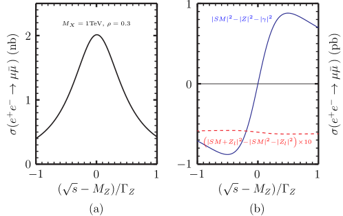
Figure 1: (a) The line shape of $e^{+}e^{-}\rightarrow\mu\bar{\mu}$ cross section near the Z-pole for $M_{X}=1$TeV and $\rho=0.3$. (b) The SM photon-$Z$ interference, and the $Z_{l}$-SM interference.

We parameterize the cross section as

$$\frac{d\sigma}{d\cos{\theta}}=\frac{\pi\alpha^{2}}{2s}\left[A(1+\cos^{2}{\theta})+B\cos{\theta}\right]\,.$$ (46)

Then $A_{FB}$ is given by

$$\begin{split}A_{FB}&=\frac{\int^{1}_{0}d\cos{\theta}\frac{d\sigma}{d\cos{\theta}}-\int^{0}_{-1}d\cos{\theta}\frac{d\sigma}{d\cos{\theta}}}{\int^{1}_{-1}d\cos{\theta}\frac{d\sigma}{d\cos{\theta}}}\\ &=\frac{3B}{8A}\,,\end{split}$$ (47)

where $A,B$ can be easily read from Eq.(44). $A_{FB}$ is center-of-mass energy dependent.

At the Z pole, we have

$$A_{FB}=\frac{3}{4}\frac{(g_{R}^{2}-g_{L}^{2})^{2}}{(g_{R}^{2}+g_{L}^{2})^{2}}\sim 0.01695$$ (48)

by using $s_{W}^{2}=0.2311$. It is accidentally small because $s_{W}^{2}$ is very close to $1/4$. It is interesting to note that the $Z_{\mathfrak{l}}$ exchange induces a universal positive contribution to all $A_{FB}^{l}$ for SM charged leptons at the Z-pole. This can be understood because as follows. First, as $Z_{\mathfrak{l}}$ is heavier than $M_{Z}$, it gives a destructive interference to the symmetric $D_{\gamma l}$ term and reduces $A$. Second, the asymmetric $(g_{L}-g_{R})^{2}(\gg(g_{L}^{2}-g_{R}^{2})^{2})$ term from $Z_{l}-$SM interference increases $B$ in Eq.(47). On the other hand, the $A_{FB}^{q}$ for SM quarks receive no such contributions. Therefore, with the presence of $Z_{\mathfrak{l}}$ and $M_{X}>M_{Z}$, $\widetilde{A}_{FB}^{l}>\widetilde{A}_{FB}^{q}$, where $\widetilde{A}_{FB}\equiv A_{FB}/A_{FB}^{SM}$, is a robust prediction. For $A_{FB}^{b}$, the LEP experimental value is measured to be $0.0992(16)$, and the SM expectation is $0.1031(3)$ Patrignani et al. (2016) by using the above value of $s_{W}$ and all other SM parameters input from the global electroweak precision fit. Or roughly speaking, $\widetilde{A}_{FB}^{l}/\widetilde{A}_{FB}^{b}=1.0393\pm 0.0164$.

However, taking into account the mass bound, Eq.(42), only a $10.7$ TeV $Z_{\mathfrak{l}}$ with $\rho\sim 36.3$ can explain this difference between lepton and quark sector at $2\sigma$ level. In other words, with $g_{\mathfrak{l}}\sim 6e$ one can account for this discrepancy. Certainly, whether this difference is due to $Z_{\ell}$ will be clarified at a future Z-factory option $e^{+}e^{-}$ colliders.

Beyond the Z-pole and for $M_{Z}\ll\sqrt{s}\ll M_{X}$,

$$\begin{split}A_{FB}&\sim\frac{3}{4}\,\frac{(g_{R}^{2}-g_{L}^{2})^{2}+2(s_{W}c_{W})^{2}(g_{R}-g_{L})^{2}}{4(s_{W}c_{W})^{4}+(g_{R}^{2}+g_{L}^{2})^{2}+2(s_{W}c_{W})^{2}(g_{R}+g_{L})^{2}}\\ &\sim 0.4691\,.\end{split}$$ (49)

At the $Z_{\mathfrak{l}}$ pole, the asymmetry is small due to the vector coupling nature of $Z_{\mathfrak{l}}$ and it becomes

$$\begin{split}A_{FB}&\sim\frac{3}{4}\,\frac{(g_{R}-g_{L})^{2}}{(g_{R}+g_{L})^{2}+2(s_{W}c_{W})^{2}\frac{2}{3\alpha}}\\ &\sim 8.83\times 10^{-6}\end{split}$$ (50)

by using Eq.(43). It is interesting that the above three values are not sensitive to $\rho$. Finally, for $\sqrt{s}\gg M_{X}$

$$\frac{4}{3}A_{FB}\sim$$ (51)

$$\frac{(g_{R}^{2}-g_{L}^{2})^{2}+2\bar{\rho}(s_{W}c_{W})^{2}(g_{R}-g_{L})^{2}}{4(s_{W}c_{W})^{4}\bar{\rho}^{2}+(g_{R}^{2}+g_{L}^{2})^{2}+2\bar{\rho}(s_{W}c_{W})^{2}(g_{R}+g_{L})^{2}}\,,$$

where $\bar{\rho}=1+\rho$. We give a plot of $A_{FB}$, Fig.2, for $M_{X}=2$ TeV and $\rho=0.3,1.0$.

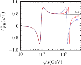
Figure 2: The $A_{FB}$ vs $\sqrt{s}$ with $M_{X}=2$TeV. The black curve is for the SM, and the red(blue) curve is for a $Z_{\mathfrak{l}}$ with $\rho=0.3(1.0)$.

The $\sqrt{s}$ dependent $A_{FB}$ provides an important handle to probe the new heavy gauge boson. It is especially useful for the planned linear colliders. For example, the CLIC has plans for 2-staged intermediate energy at $\sqrt{s}=0.5,1.4(1.5)$ TeV before reaching its ultimate $3$TeV goalLebrun et al. (2012). At each new stage, it is able to tune down the energy by about factor 3 without losing the luminosity. One might be able to see the effect of new gauge boson in the $A_{FB}$ even if $Z_{\ell}$ is too heavy to be produced on shell.

V.4 Muon $g-2$

The $Z_{\mathfrak{l}}$ contribution to the muon anomalous moment can be easily calculated to be

$$\Delta a_{\mu}=\frac{\alpha}{3\pi}\rho\left(\frac{m_{\mu}^{2}}{M_{X}^{2}}\right)\,.$$ (52)

Using the value $a_{\mu}^{exp}-a_{\mu}^{th}=2.88\times 10^{-9}$Patrignani et al. (2016) and requiring that $\Delta a_{\mu}$ is smaller than that, we obtain the constraint $M_{X}>54.5\sqrt{\rho}$ GeV. The helicity flip factor severely curtails the sensitivity of $a_{\mu}$ to $M_{X}$. The new exotic scalars have contributions to $\Delta a_{\mu}$ as well. Since their masses have to be heavier than $\sim 0.8$TeV, those contributions are negligible. However, this limit can not compete with Eq.(42). For a recent review of the connection between $a_{\mu}$ and the new physics, seeLindner et al. (2018).

V.5 Møeller Scattering

The exchange of $Z_{\mathfrak{l}}$ will interfere with the SM $Z,\gamma$ processes at the amplitude level. The leading order is free of hadronic uncertainties and hence offers a very clean sensitive probe of $Z_{\mathfrak{l}}$. Since the $Z_{\mathfrak{l}}$ admits vector coupling to the electron, it does not contribute left-right asymmetry directly. Its role in the Møeller scattering is to increase the symmetric cross section from the photon exchange diagram. The asymmetry is then reduced to

$$A_{LR} \simeq A_{LR}^{SM}\times\left[1-6\frac{\rho Q^{2}}{M_{X}^{2}}\frac{(1-y)(1-y+y^{2})}{1+y^{4}+(1-y)^{4}}\right]\,,$$ (53)

$$A_{LR}^{SM} = \frac{4G_{\mu}s}{\sqrt{2}\pi\alpha}\frac{y(1-y)}{1+y^{4}+(1-y)^{4}}\left[\frac{1}{4}-s_{w}^{2}\right]\,,$$ (54)

where $y=-\frac{t}{s}$. The asymmetry was measured to be

$$A_{LR}=131\pm 14(\mbox{stas})\pm 10(\mbox{syst})\mbox{ppb}$$ (55)

by the SLAC E158 experimentAnthony et al. (2005), where $Q^{2}=0.026(GeV)^{2}$, $y=0.6$, thus $A_{LR}^{SM}=1.47\times 10^{-7}$. By taking the 95%C.L. limit, $-0.337<\frac{\delta A_{LR}}{A_{LR}}<0.122$. Due to the stringent limits from Eq.(42), the $Z_{\mathfrak{l}}$ contribution to $\frac{\delta A_{LR}}{A_{LR}}$ has no significance at all.

V.6 $Z_{\mathfrak{l}}$ production at the LHC

If energetically allowed, $Z_{\mathfrak{l}}$ can be produced at the LHC via the radiaitive Drell-Yan process as depicted in Fig.(3).

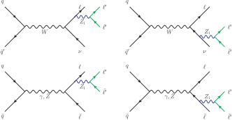
Figure 3: Drell-Yan production of $Z_{\mathfrak{l}}$.

The final states will be two pairs of leptons with different flavors in which one pair constitutes a resonance. E.g. $\mu^{+}\mu^{-}$ and $e^{+}e^{-}$ pairs and either pair coming from on-shell $Z_{\mathfrak{l}}$ decay. Another signal will be three leptons plus missing energy . A spectacular example will be a $\mu^{+}\mu^{-}$ and an $e^{+}e^{-}$ pair with either pair resulting from $Z_{\mathfrak{l}}$ decay. Neither signatures will have no jet activities.

Here, just for illustration purpose, we consider the signal $pp\rightarrow e^{+}e^{-}Z_{\mathfrak{l}}\rightarrow e^{+}e^{-}+(\mu\bar{\mu})$, and there is a sharp resonance peak of muon pair invariant mass at $M_{X}$. The SM background is $pp\rightarrow e^{+}e^{-}\mu^{+}\mu^{-}$ with the $m_{\mu\bar{\mu}}\sim M_{X}$. We evaluate the cross section of $pp\rightarrow e^{+}e^{-}Z_{\mathfrak{l}}$ at LHC for three CM energies by the program CalcHepBelyaev et al. (2013) with the CTEQ6l1 PDF setPumplin et al. (2002). The SMBG are also evaluated by CalcHep with a cut that $m_{\mu\bar{\mu}}\in(M_{X}-50GeV,M_{X}+50GeV)$. The numbers are listed in Tab.3.

$\frac{\sqrt{s}}{\mathrm{TeV}}$		$\frac{M_{X}}{\mathrm{TeV}}=0.5$	$\frac{M_{X}}{\mathrm{TeV}}=1.0$	$\frac{M_{X}}{\mathrm{TeV}}=2.0$	$\frac{M_{X}}{\mathrm{TeV}}=5.0$
14	$\frac{\sigma}{g_{l}^{2}}$	$5.4\times 10^{-5}$	$1.7\times 10^{-6}$	$1.9\times 10^{-8}$	$9.8\times 10^{-13}$
	$\sigma_{BG}$	$2.2\times 10^{-5}$	$1.4\times 10^{-6}$	$5.4\times 10^{-8}$	$6.2\times 10^{-11}$
	$\frac{\bar{w}_{max}}{\mathrm{TeV}}$	$0.61$	$0.43$	-	-
30	$\frac{\sigma}{g_{l}^{2}}$	$2.6\times 10^{-4}$	$1.5\times 10^{-5}$	$5.1\times 10^{-7}$	$1.0\times 10^{-9}$
	$\sigma_{BG}$	$6.8\times 10^{-5}$	$7.1\times 10^{-6}$	$4.2\times 10^{-7}$	$5.7\times 10^{-9}$
	$\frac{\bar{w}_{max}}{\mathrm{TeV}}$	$1.02$	$0.85$	-	-
100	$\frac{\sigma}{g_{l}^{2}}$	$1.7\times 10^{-3}$	$1.5\times 10^{-4}$	$1.1\times 10^{-5}$	$1.8\times 10^{-7}$
	$\sigma_{BG}$	$3.0\times 10^{-4}$	$3.2\times 10^{-5}$	$2.8\times 10^{-6}$	$7.6\times 10^{-8}$
	$\frac{\bar{w}_{max}}{\mathrm{TeV}}$	$1.79$	$1.85$	$1.83$	-

Table 3: The $pp\rightarrow e^{+}e^{-}Z_{l}$ cross section normalized by $g_{l}^{2}$ and the SM BG. The cross sections are in $(pb)$, and $\bar{w}_{max}$ are in TeV.

We use $S/\sqrt{B}=3$ and an integrated luminosity ${\cal L}_{0}=3000(fb)^{-1}$ as the benchmark limit of detecting a $Z_{l}$ at the LHC. Then,

$$\begin{split}3&=\frac{\sigma(pp\rightarrow e^{+}e^{-}Z_{\mathfrak{l}}(\mu\bar{\mu}))Br(Z_{\mathfrak{l}}\rightarrow\mu\bar{\mu})\times{\cal L}_{0}}{\sqrt{\sigma_{BG}\times{\cal L}_{0}}}\\ &=\frac{2}{9}\sqrt{\frac{{\cal L}_{0}}{\sigma_{BG}}}\,\left(\frac{\sigma}{g_{\mathfrak{l}}^{2}}\right)\,g_{\mathfrak{l}}^{2}\,.\end{split}$$ (56)

The corresponding highest lepton number breaking scale we can probe is $\bar{w}^{2}_{max}=(2/27)\sqrt{{\cal L}_{0}/\sigma_{BG}}\times(\sigma/g_{\mathfrak{l}}^{2})M_{X}^{2}$, which is also displayed in Tab.3. The LHC14, LHC30, and LHC100 have the potential to probe the lepton-number violating scales up to $\sim 0.5,1.0$, and $2.0$ TeV, respectively.

VI Radiative Seesaw mass for $\nu_{L}$

The Feynman diagrams for radiative $\nu_{L}$ mass generation are depicted in Fig.4 which are given in the weak eigenbasis. They fill in the upper left-hand block of zeros in Eq.(18) .

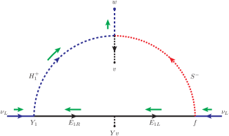
Figure 4: one-loop $\nu_{e}\,\nu_{e}$ mass term generation. Green arrows show the flow of lepton charge

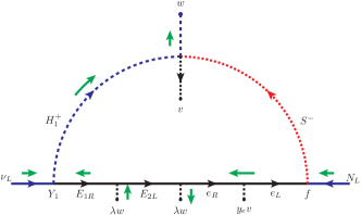
Figure 5: one-loop $\nu_{eL}\,N$ mass term generations. Green arrows show the flow of lepton charge.

In the limit that the charged $H_{1},S$ scalars are heavier than the leptons, we get

$$M_{11}=\frac{f(Y_{1}v)(\lambda_{1\ell}w)m_{e}}{16\pi^{2}(m_{1}^{2}-m_{S}^{2})}\ln{\left(\frac{m_{1}^{2}}{m_{S}^{2}}\right)}\,,$$ (57)

where we have used $Yv=m_{e}$ as explained above. $M_{11}$ will be the upper leftmost entry in Eq.(18). Similarly, we get radiative correction to $M_{12,21}$, Fig.5. Clearly, these are much smaller than $\bar{\lambda}w$. Other than providing a Majorana mass for the active neutrino $\nu_{e}$, they also transform the Dirac neutrino $N$ into a pseudo-Dirac one. Numerically, the splitting will be undetectably small for all practical purposes, and we can treat the $N$ as a Dirac neutrino. Assuming that there is no outstanding hierarchy between $m_{1}$ and $m_{S}$, then one expects the combination $w/(m_{1}^{2}-m_{S}^{2})\ln(m_{1}^{1}/m_{S}^{2})\simeq w\sim{\cal O}(\mbox{TeV})$. Plugging in the values, the resulting active neutrino mass is around $m_{\nu}\sim fY_{1}\lambda_{1\ell}\times 10^{3}$ eV. And the sub-eV neutrino mass can be easily achieved with $f,Y_{1},\lambda_{1\ell}\sim{\cal O}(0.1)$ without prominent fine-tuning.

VII Phenomenology of $E,N$

Even if the exotic leptons are too heavy to be produced by current or near-future colliders, they can have important effects at current energies. The notable ones are the electroweak oblique parameters $S,T$Peskin and Takeuchi (1990, 1992), and the decay $h\to\gamma\gamma$.

VII.1 Oblique parameters $S,T$

It is well known that the oblique parameters $S$ and $T$ constraint heavy fermions that carry SM quantum numbers. In this case, they constrain the mass differences of the lepton pairs $E,N$ as well as the number of such pairs. Explicitly, for each generation we have

$$\triangle T = \frac{1}{16\pi s_{w}^{2}}\sum_{i=1,2}\frac{M_{E_{i}}^{2}}{M_{W}^{2}}\left(1+x_{i}+\frac{2x_{i}}{1-x_{i}}\ln x_{i}\right)\,,$$ (58)

$$\triangle S = \frac{1}{6\pi}\sum_{i=1,2}\left(1+\ln x_{i}\right)\,,$$ (59)

where $x_{i}=M_{N_{i}}^{2}/M_{E_{i}}^{2}$. When the mass splitting between $E_{i}$ and $N_{i}$ is small comparing to their masses,

$$\triangle T \sim \frac{1}{12\pi s_{w}^{2}M_{W}^{2}}[(M_{N_{1}}-M_{E_{1}})^{2}+(M_{N_{2}}-M_{E_{2}})^{2}]\,,$$

$$\triangle S \sim \frac{1}{3\pi}\left[1+\frac{M_{N_{1}}-M_{E_{1}}}{M_{E_{1}}}+\frac{M_{N_{2}}-M_{E_{2}}}{M_{E_{2}}}\right]\,,$$ (60)

for each generation. The doublet $H_{1}$ provides contribution

$$\triangle T = \frac{1}{16\pi s_{w}^{2}}\frac{M_{H^{+}}^{2}}{M_{W}^{2}}\frac{1}{z}\left[1+z+\frac{2z}{1-z}\ln z\right]\,,$$ (61)

$$\triangle S = -\frac{1}{12\pi}\ln z\,,$$ (62)

where $z\equiv M_{H^{+}}^{2}/M_{H_{1}^{0}}^{2}$. Note that $\triangle T$ from fermions and doublet scalar are both positive, but $\triangle S$ from the doublet scalar can be either positive or negative. From the Particle Data Group, we have $S_{data}<0.22$ and $T_{data}<0.27$ at 95% C.L.Patrignani et al. (2016)

To see how these will restrict the parameters of our model, we begin by taking $z=1$; i.e. the neutral and charged components of $H_{1}$ are degenerate. This implies that the mixing of $H_{1}$ with all other scalars is negligible. Then, the scalar contributions to $\triangle T$ and $\triangle S$ are vanishing. For simplicity, we also assume the masses of $E_{+}$ and $E_{-}$ are equal and their counterparts for $\mu$ and $\tau$ families are also the same. From Eq.(59) we see that the new isodoublet chiral leptons cannot have degenerate upper and lower components; otherwise it runs afoul of $S_{data}$. The splitting between the neutral and charged components that saturates $T_{data}$ is given by

$$x=0.73$$ (63)

where we have dropped the subscript $i$. Using Eq.(58) and $T_{data}$, we obtain $M_{E}\leq 350$ GeV. The above values are to be taking as a demonstration that the stringent constrains of oblique corrections can be satisfied with new lepton masses in the range of 350 GeV, the vertical dash blue line in Fig.6. This is well above limit form the charged lepton searches of $>100.8$ GeV, the vertical dash red line in Fig.6, given in PDGPatrignani et al. (2016) .

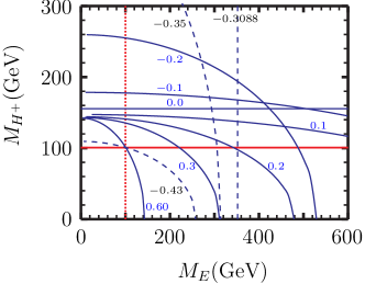
Figure 6: Contours from $\triangle S$ and $\triangle T$ constraints for different $\ln x$. For a given $\ln x$, the allowed masses region is above the direct search bound on $M_{H^{+}}$, the horizontal red line, to the right of the direct search bound on $M_{E}$, the vertical dashed red line, and to the lower left of the blue (dash)curve.

We can also of take the limit that the $E$ and $N$ are degenerate, i.e. all $x=1$. Then Eq.(59) yields $\triangle S\simeq.32$. Then, it will require $H_{1}$ doublet with $\ln z\simeq 3.71$ to bring it within the experimental bound since scalars give a negative contribution (see Eq.(62)). The scalars will then be the sole contributors to $\triangle T$. A similar calculation gives an upper bound on the mass of $H^{+}$ to be 155 GeV, the horizontal blue line in Fig.6. This value is also larger than the direct search bound on charged scalars, the horizontal red line in Fig.6. The large splitting between $H^{+}$ and $H_{1}^{0}$ implies that some if not all of the parameters $\kappa_{H_{1}S},\kappa_{\Phi_{i}H_{1}}$ and $\mu_{3}$ in Eq.(9)are large.

Notice that since $z$ is large, we have $M_{H_{1}^{0}}\simeq 24.4$ GeV. In general, it can mix with the SM Higgs boson, but we have seen that this mixing is constrained to be small. In the interaction basis, which is good for small mixings, it does not couple to quarks, and it has no couplings to gluons to one-loop. Because of this, it will not run into problem at the LHC. Neutral scalars in the mass range of $10-100$ GeV is notoriously difficult to detect. The challenges and a possible signal for probing this at the LHC was discussed in Chang et al. (2018a). Additionally, a more promising avenue of exploring this at a future $e^{+}e^{-}$ collider is given in Chang et al. (2018b).

From the above limiting case, it is easy to see that if $\ln x>-0.3088$ the doublet $H_{1}$ will have to play a role in satisfying the oblique corrections bounds. For $\ln x=-0.3088$, it is the vertical dashed blue line in Fig.6. It is more realistic to assume finite mass splittings between the isodoublets for both leptons and scalars. As an illustration we take $\ln x=-0.2$, then the masses of $M_{E}$ and $M_{H^{+}}$ will satisfy a contour given by

$$.0062\left(\frac{M_{E}}{M_{W}}\right)^{2}+.0259\left(\frac{M_{H^{+}}}{M_{W}}\right)^{2}\leq 0.27.$$ (64)

The allowed regions of $M_{E}$ and $M_{H^{+}}$ for different $\ln x$ are displayed in Fig.6. If both experimental lower bounds on $M_{E},M_{H^{+}}$ are met, one can see that the range of $\ln x$ is $-0.43572<\ln x<0.6053$, and it implies that $0.80<(M_{N}/M_{E})<1.35$ and $0.47<(M_{H^{+}}/M_{H^{0}})<241.0$ if a universal $x_{i}$ is assumed. Moreover, for $\ln x>-0.1$, a light neutral scalar with mass $M_{H^{0}}<50$ GeV is expected.

Before closing this section, we remark that it is well-known that the constraint from $\triangle T$ can be largely loosen by introducing an $SU(2)$ triplet with a small VEV so that the tree-level electroweak $\rho$-parameter is less than unity. However, for the minimal setup, we do not further into such discussion. See Chang and Ng (2018) for utilizing a triplet Higgs for neutrino mass generation and relaxing the $\Delta T$ constraint in this model.

VII.2 Impact on Higgs decays

VII.2.1 Higgs to two photons.

The SM Higgs to the di-photon vertex is generated at the one-loop level with dominant contributions from $W^{\pm}$ and top quark running in the loop. In our model, there are six new charged leptons; a $E_{1},E_{2}$ pair for each of the three generations, and two new charged scalars, $H_{1}^{\pm}$ and $S^{\pm}$. These charged fields mix among themselves, and one needs to know every parameter for the actual mass diagonalization. However, with assumptions on the masse ranges of these charged particles, a general discussion is sufficient to draw qualitative conclusions.

In the mass basis, we can parameterize the Yukawa couplings and cubic couplings to the SM Higgs as

$${\cal L}\supset-\sum_{i=1}^{6}y_{E_{i}}\bar{E}_{i}E_{i}h-\sum_{i=1,2}\lambda_{i}M_{W}hH_{i}^{+}H_{i}^{-}\,.$$ (65)

These new electrically charged degrees of freedom enter the one-loop triangle diagram and modify the width of the SM Higgs di-photon decay. This is given by Djouadi (2008)

$$\Gamma(H\rightarrow\gamma\gamma)={G_{F}\alpha^{2}M_{H}^{3}\over 128\sqrt{2}\pi^{3}}\left|F_{1}(\tau_{W})+\frac{4}{3}F_{1/2}(\tau_{t})\right.$$

$$+\sum_{j=1,2}\lambda_{i}\frac{M_{W}^{2}}{g_{2}M_{H_{i}}^{2}}F_{0}(\tau_{H_{i}})$$

$$\left.+\sum_{i=1}^{6}y_{E_{i}}\frac{2M_{W}}{g_{2}M_{E_{i}}}F_{1/2}(\tau_{E_{i}})\right|^{2}\,,$$ (66)

where $\tau_{i}\equiv(m_{H}/2m_{i})^{2}$, and

$$F_{0}(\tau) = -[\tau-f(\tau)]/\tau^{2}\,,$$

$$F_{1/2}(\tau) = 2[\tau+(\tau-1)f(\tau)]/\tau^{2}\,,$$

$$F_{1}(\tau) = -[2\tau^{2}+3\tau+3(2\tau-1)f(\tau)]/\tau^{2}\,,$$ (67)

with

$$f(\tau)=\left\{\begin{array}[]{ll}\left[\sin^{-1}\sqrt{\tau}\right]^{2}\,,&\mbox{if}\,\tau\leq 1\\ -\frac{1}{4}\left[\log{1+\sqrt{1-1/\tau}\over 1-\sqrt{1-1/\tau}}-i\pi\right]^{2}\,,&\mbox{if}\,\tau>1\,.\\ \end{array}\right.$$ (68)

For $m_{i}\gg M_{H}/2=62.5$GeV, we have the following expansions around $\tau=0$:

$$F_{0}(\tau) \sim \frac{1}{3}+\frac{8}{45}\tau+{\cal O}(\tau^{2})\,,$$

$$F_{1/2}(\tau) \sim \frac{4}{3}+\frac{14}{45}\tau+{\cal O}(\tau^{2})\,,$$

$$F_{1}(\tau) \sim -7-\frac{22}{15}\tau+{\cal O}(\tau^{2})\,.$$ (69)

Plugging in the numbers, the di-photon decay width reads

$$\Gamma(H\rightarrow\gamma\gamma)=\left.{G_{F}\alpha^{2}M_{H}^{3}\over 128\sqrt{2}\pi^{3}}\times\right|-8.324+1.834$$

$$+8.3\times 10^{-4}(1.3\times 10^{-2})\times\lambda_{2}+0.087(0.42)\times\lambda_{1}$$

$$\left.+\sum_{i=1}^{6}0.32(3.64)\times y_{E_{i}}\right|^{2}$$ (70)

for $M_{E_{i}}=1000(100)$GeV, $M_{H_{2}}=2.0(0.5)$TeV, and $M_{H_{1}}=200(100)$GeV. The first two numbers are the dominate SM contributions from $W^{\pm}$ and the top quark, respectively. Since we expect $|y_{E_{i}}|\sim m_{l}/v_{h}\ll 1$, even for the new leptons (see Sec. III), the charged leptons contribution can be ignored. If the second charged scalar is heavy, its contribution can be ignored, too, even taking $\lambda_{2}\sim{\cal O}(1)$. Therefore, only the light charged scalar with mass in the range of 100 to 200 GeV matters. The gluon fusion is the dominant SM Higgs production channel at the LHC, and it does not receive any modification. The signal strength of $pp\rightarrow h\rightarrow\gamma\gamma$ at the LHC is therefore

$$\mu_{\gamma\gamma} \simeq \Gamma(H\rightarrow\gamma\gamma)/\Gamma(H\rightarrow\gamma\gamma)_{SM}$$ (71)

$$\sim 1-(0.03-0.13)\times\lambda_{1}\,.$$

Comparing with the experiment data $\mu_{\gamma\gamma}=1.18(+0.17-0.14)$ Sirunyan et al. (2018), we conclude that it is safe even the light charged Higgs has a coupling $|\lambda_{1}|\sim{\cal O}(1)$. This is in agreement with the general analysis given in Chang et al. (2012).

VII.2.2 Higgs to 4 fermions

For notational simplicity, here we denote $h_{1}\equiv\Re(H_{1}^{0})$ and $a_{1}\equiv\Im(H_{1}^{0})$. If $h_{1}$ ( or $a_{1}$ ) is lighter than half the mass of the SM Higgs, $h_{SM}$, then we can have

$$h_{SM}\rightarrow 2h_{1}(2a_{1})\rightarrow\bar{\ell_{i}}\ell_{i}+\bar{\ell_{j}}\ell_{j}\,.$$ (72)

The decay width is

$$\Gamma(h_{SM}\rightarrow h_{1}h_{1}(a_{1}a_{1}))=\frac{v^{2}(\kappa_{2}+\kappa_{3})^{2}}{32\pi M_{H}}\left(1-\frac{4m_{1}^{2}}{M_{H}^{2}}\right)^{\frac{1}{2}}\,,$$ (73)

where $M_{H}(=125\mbox{GeV})$ and $m_{1}$ are the masses of $h_{SM}$ and $h_{1}(a_{1})$, respectively. We have neglected term involving off-diagonal mixing of neutral scalars. The dominant decay mode for $h_{1}(a_{1})$ is model dependent. The current bound on the mixing squared between $h_{SM}$ and $h_{1}$ is about $\lesssim 10^{-2}$ for $10<m_{1}<40$ GeV from LEP2Barate et al. (2003). For $Y_{1}\sim O(0.1)$, as expected from the radiative neutrino masses, the effects from the mixing with SM Higgs cannot compete with those from the direct Yukawa interaction, Eq.(19). Therefore, for scenario A , the main decay channel will be $h_{1}(a_{1})\rightarrow\bar{\ell}\ell$ with $\ell=e,\mu,\tau$. The signal will be SM Higgs decays into 2 charged leptons pairs with both invariant masses peaking at the unknown $m_{1}$.

For scenario B, $h_{1}(a_{1})$ has only off-diagonal couplings to SM lepton and a heavy lepton; see Eq.(23). The dominant decay of light $h_{1}(a_{1})$ is expected to be due to mixing with the $h_{SM}(\Im(H_{0}^{0}))$ which then decays into a fermion pair. Therefore, $\bar{b}b$ will be the dominate final state if $m_{1}>10$ GeV.

For the general case, in between scenario A and B, we expect the mixing element $|U_{12}|^{2}<0.13$, from unitarity and $|U_{11}|^{2}>0.87$ Aad et al. (2016), to be small but non-vanishing.

VII.3 Colliders production and decay of exotic leptons

For both scenarios (A) and (B), the SM gauge interaction allows $E_{\pm}\rightarrow W^{-}N_{\pm},W^{-}N_{\mp}$, and $N_{+}\rightarrow N_{-}Z$ if $M_{N}<M_{E}$ is assumed. We consider the decay, $E_{\pm}\rightarrow NW^{-}$, of a heavy Dirac $N$ for simplicity. The decay width is calculated to be

$$\Gamma_{E_{\pm}\rightarrow NW^{-}} = {G_{F}M_{E}^{3}\over 8\sqrt{2}\pi}\lambda_{cm}(x_{N},x_{w})f(x_{w},x_{N})$$

$$f(x,y) = x(1+y-2x\mp 6\sqrt{x})+(1-y)^{2}$$ (74)

where $\lambda_{cm}(y,z)=\sqrt{1+y^{2}+z^{2}-2(y+z+yz)}$, $x_{w}=(M_{W}/M_{E})^{2}$, and $x_{N}\equiv(M_{N}/M_{E})^{2}$. For $M_{E}\gg M_{W}$, or $x_{w}\ll 1$, the width becomes

$$\Gamma_{E_{\pm}\rightarrow NW^{-}}\simeq{G_{F}M_{E}^{3}\over 8\sqrt{2}\pi}(1-x_{N})^{3}\,.$$ (75)

As discussed in Sec.VII.1, the oblique corrections requires that $\ln x_{N}>-0.4357$, which implies that

$$\Gamma_{E_{\pm}\rightarrow NW^{-}}<14.45\times\left({M_{E}\over 1\mbox{TeV}}\right)^{3}\,\mbox{GeV}\,.$$ (76)

On the other hand, if $M_{N}>M_{E}$, the decay width of $N$ takes a similar form with $M_{E}\leftrightarrow M_{N}$,

$$\Gamma_{N\rightarrow E_{\pm}W^{+}}\simeq{G_{F}M_{N}^{3}\over 8\sqrt{2}\pi}(1-x_{N}^{-1})^{3}\,.$$ (77)

Similarly, from that $\ln x_{N}<0.6053$,

$$\Gamma_{N\rightarrow E_{\pm}W^{-}}<30.72\times\left({M_{N}\over 1\mbox{TeV}}\right)^{3}\,\mbox{GeV}\,.$$ (78)

From the above discussion, unless the leptons are nearly degenerate, the decays of $E_{\pm}$ or $N$ are expected to be prompt.

Next, we turn our attention to the heavy lepton decay via the Yukawa interaction with $H_{1}$. Let’s consider a general case with two fermions $F,f$, and a scalar $\phi$. The scalar field $\phi$ could be either neutral or charged. Assume that they admit a Yukawa interaction which is parameterized as ${\cal L}\supset\bar{F}(s+a\gamma^{5})f\phi+h.c.\,$. If kinematics allowed, the decay channel $F\rightarrow f\phi$ opens and the width is calculated to be

$${\lambda_{cm}(x_{f},x_{\phi})M\over 16\pi} \left[(1+x_{f})^{2}|s|^{2}\right.$$

$$\left.+(1-x_{f})^{2}|a|^{2}-x_{\phi}(|s|^{2}+|a|^{2})\right]\,,$$

where $M$ is the mass of $F$, $x_{f}=(m_{f}/M)^{2}$, and $x_{\phi}=(m_{\phi}/M)^{2}$. For the cases that $M,m_{f}\gg m_{\phi}$, the decay width becomes

$$\Gamma(F\rightarrow f\phi)\simeq\frac{M}{16\pi}(1-x_{f})\left[(1+x_{f})^{2}|s|^{2}+(1-x_{f})^{2}|a|^{2}\right]\,.$$ (80)

The relevant fields and Yukawa couplings in our model are collected and listed in Tab.4. One can read the precise expression by using Eq.(VII.3) and Tab.4. Roughly speaking, the decay widthes are about $\sim(Y_{1}^{2}/64\pi)M$, or numerically $\sim 0.05\times(Y_{1}/0.1)^{2}\times(M/1\mbox{TeV})$ GeV, where $M$ is the mass of $E_{\pm}$ or $N$. In general, this decay width is much smaller than that from the decay with a SM $W^{\pm}$ boson in the final states. Note that in scenario-B, $N$ does not have the tree-level two-body decays via the Yukawa interaction with $H_{1}$. However, if the mass of the charged scalar $S^{\pm}$ is less than $M_{N}$, then the decay $N\rightarrow e^{+}S^{-}$ is possible. Otherwise $N$ will have only three-body decays. For $M_{N}<M_{E}$, there is another chain with an intermediate virtual $E$; for example, $N\rightarrow W^{+}E^{*}\rightarrow W^{+}h_{1}e^{-}$. We shall use the superscript “$*$” to denote off-shell particles.

scenario	$F$	$f$	$\phi$	$s$	$a$
	$E_{\pm}$	$e$	$h_{1}$	$0$	$-\frac{Y_{1}}{2\sqrt{2}}$
(A)	$E_{\pm}$	$e$	$a_{1}$	$-\frac{iY_{1}}{2\sqrt{2}}$	$0$
	$E_{\pm}$	$\nu$	$H_{1}^{-}$	$\frac{Y_{1}}{4\sqrt{2}}$	$-\frac{Y_{1}}{4\sqrt{2}}$
	$N$	$e$	$H_{1}^{+}$	$-\frac{Y_{1}}{4}$	$-\frac{Y_{1}}{4}$
	$E_{\pm}$	$e$	$h_{1}$	$\frac{Y_{1}}{4}$	$-\frac{Y_{1}}{4}$
(B)	$E_{\pm}$	$e$	$a_{1}$	$-\frac{iY_{1}}{4}$	$\frac{iY_{1}}{4}$
	$E_{\pm}$	$\nu$	$H_{1}^{-}$	$\frac{Y_{1}}{2\sqrt{2}}$	$-\frac{Y_{1}}{2\sqrt{2}}$

Table 4: The $H_{1}$ Yukawa couplings between the heavy leptons and the SM ones in our model. The heavy neutrino is assumed to be Dirac.

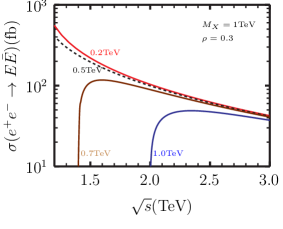
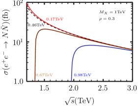
Figure 7: (a) The $E\bar{E}$, and (b)$N\bar{N}$ production cross sections v.s $\sqrt{s}$ at an $e^{+}e^{-}$ collider. The masses of $E(N)$ are labeled next to the curves.

The heavy leptons can be pair produced at the $e^{+}e^{-}$ colliders. For simplicity, we assume that $E_{+}$ and $E_{-}$ are nearly degenerate so that they are hard to be distinguished experimentally, and we collectively denote the states as $E\equiv E_{+}\sim E_{-}$. For $\sqrt{s}\gg M_{Z}$ and away from the $Z_{\ell}$ pole, the production cross section per generation for scenario-(B) can be calculated to be

$$\sigma(e^{+}e^{-}\rightarrow E\bar{E})\simeq$$

$$2{4\pi\alpha^{2}\over 3s}\sqrt{1-4x_{E}}\left\{\left(1+{\rho s\over s-M_{X}^{2}}\right)^{2}(1+2x_{E})\right.$$

$$+{(g^{e}_{L})^{2}+(g^{e}_{R})^{2}\over 4(s_{W}c_{W})^{4}}\left[(1-x_{E})((g^{E}_{L})^{2}+(g^{E}_{R})^{2})+6x_{E}g^{E}_{L}g^{E}_{R}\right]$$

$$+\left.{(g^{e}_{L}+g^{e}_{R})\over 2(s_{W}c_{W})^{2}}(g^{E}_{L}+g^{E}_{R})\left(1+{\rho s\over s-M_{X}^{2}}\right)\left(1-x_{E}\right)\right\}$$ (81)

where $x_{E}\equiv M_{E}^{2}/s$, $g^{E}_{L}\simeq g^{e}_{L}=-1/2+s_{W}^{2}$, $g^{E}_{R}\simeq g^{e}_{R}=s_{W}^{2}$. The first factor 2 represents the incoherent sum from the contribution of the two heavy Dirac charged leptons. For example, if $\{M_{E_{+}},M_{E_{-}}\}=\{200,180\}$GeV, $\rho=0.3$, and $M_{X}=1$TeV, the production cross section of 2 charged leptons are $556.0(83.2)$ fb for $\sqrt{s}=1.2(2.2)$TeV, see Fig.7(a). Similarly, the heavy $N$ can be pair produced through the s-channel process mediated by $Z,Z_{\ell}$, and the production cross section for each generation is

$$\sigma(e^{+}e^{-}\rightarrow N\bar{N})\simeq$$

$${4\pi\alpha^{2}\over 3s}\sqrt{1-4x_{N}}\left\{\left({\rho s\over s-M_{X}^{2}}\right)^{2}(1+2x_{N})\right.$$

$$+{(g^{e}_{L})^{2}+(g^{e}_{R})^{2}\over 8(s_{W}c_{W})^{4}}(1+2x_{N})$$

$$+\left.{(g^{e}_{L}+g^{e}_{R})\over 2(s_{W}c_{W})^{2}}\left({\rho s\over s-M_{X}^{2}}\right)\left(1-x_{N}\right)\right\}$$ (82)

For example, if $M_{N}=170$GeV, $\rho=0.3$, and $M_{X}=1$TeV, the production cross section of $N\bar{N}$ pair are $94.0(12.4)$ fb for $\sqrt{s}=1.2(2.2)$TeV, see Fig.7(b).

At the LHC, the heavy leptons can be produced via the photon and(or) W-/Z-boson Drell-Yan process. Therefore, the production cross sections are independent of the $Z_{\ell}$ mass and the $U(1)_{\ell}$ gauge couplings. Since a full-fledged collider study is beyond the scope of this paper, only the production cross-section are considered here. Three sets of $(M_{E_{+}},M_{E_{-}})$ are considered as the benchmarks with the assumption that their mass differences are sub-electroweak. For each benchmark, $M_{N}$ is chosen to meet the constraint from the electroweak precision; with $|\ln x|<\{0.3,0.15,0.05\}$ for $M_{E_{+}}=\{200,500,1000\}$ GeV, respectively. The production cross sections are evaluated by CalcHep and listed in Table5 and Table6.

For $M_{E},M_{N}\lesssim 500$ GeV, the production cross sections are about ${\cal O}(1-100)fb$. The production of $E$ and $N$ will be followed by their decays into SM particles. The decay modes are sensitive to the masses of $E_{+},E_{-},N$ as well as the masses of the charged scalars $H_{1}^{\pm},S^{\pm}$, which in general mix. If the splitting between $E,N$ is large enough the dominant decays will be two-body modes; otherwise, they will be three-body modes. They also depend on the ordering of the $E,N$ masses. If $M_{E}>M_{S^{\pm}}$, then we have the chain

$$E\rightarrow\bar{\nu}+ S^{-}$$ (83)

where the decay of $S^{-}$ proceeds via mixing with $H_{1}^{-}$. Additionally, in scenario-(B), if $M_{E}>M_{N}$ we also have the chain

$$E\rightarrow W^{-}+ N$$

$$\downarrow$$

$$\phantom{E\rightarrow}W^{-}+ E^{(*)} +W^{+}$$ (84)

where we take the decay of $E$ to proceed via

$$E\rightarrow e+h_{1}(a_{1})\rightarrow e+\ell\bar{\ell}\,$$ (85)

if $Y_{1}$ is not too small.

Next, we examine the decays of the neutral lepton $N$. If $M_{N}>M_{E}$, the decay chain will be

$$N\rightarrow W^{+}+ E$$ (86)

Similar to the case of $E$, if $M_{N}>M_{S^{\pm}}$ the following is also available

$$N\rightarrow e^{+}+ S^{-}$$ (87)

Before one can draw any conclusion, it is crucially important to understand the SM background first. We leave the comprehensive signal and background study to a future work.

	$M_{E_{+}}$	$M_{E_{-}}$	$\bar{E}_{+}E_{+}$	$\bar{E}_{+}E_{-}+\bar{E}_{-}E_{+}$	$\bar{E}_{-}E_{-}$
set-1	$200$	$180$	$9.62\times 10^{-2}$	$4.27\times 10^{-2}$	$1.40\times 10^{-1}$
set-2	$500$	$480$	$2.76\times 10^{-3}$	$9.04\times 10^{-4}$	$3.30\times 10^{-3}$
set-3	$1000$	$950$	$9.08\times 10^{-5}$	$2.44\times 10^{-5}$	$1.21\times 10^{-4}$

Table 5: The production cross sections(in pb) at the LHC14 for one generation in scenario-B in our model. The masses of $E_{\pm}$ are in the unit of GeV.

	$M_{N}$	$\bar{N}N$	$\bar{N}E_{+}+\bar{E}_{+}N$	$\bar{N}E_{-}+\bar{E}_{-}N$
set-1	$170$	$3.68\times 10^{-1}$	$1.19\times 10^{-1}$	$5.20\times 10^{-2}$
set-1	$230$	$1.21\times 10^{-1}$	$6.90\times 10^{-2}$	$2.89\times 10^{-2}$
set-2	$460$	$7.76\times 10^{-3}$	$3.04\times 10^{-3}$	$1.04\times 10^{-3}$
set-2	$540$	$3.87\times 10^{-3}$	$2.17\times 10^{-3}$	$7.24\times 10^{-4}$
set-3	$980$	$1.93\times 10^{-4}$	$9.28\times 10^{-5}$	$2.69\times 10^{-5}$
set-3	$1020$	$1.53\times 10^{-4}$	$8.29\times 10^{-5}$	$2.37\times 10^{-5}$

Table 6: The production cross sections(in pb) at the LHC14 for one generation in scenario-B in our model. The masses of $N$ are in the unit of GeV.

VIII Conclusions

An anomaly-free gauged $U(1)_{\mathfrak{l}}$ lepton model was constructed to study the nature of lepton number. Different from previous studies in the literature, we found two solutions which are free of the anomaly for each SM fermion generation. Our solutions also do not require type-I seesaw mechanism for active neutrino mass generation. The price we pay is introducing four extra chiral fermion fields per generation. While the two solutions whose anomaly cancelation is nontrivial, look superficially similar. The fermion content of one solution is displayed in Tab.1. We have constructed the minimal scalar sector, Tab.2, such that the active neutrino masses are generated radiatively without significant fine-tuning the model parameters. Moreover, the new leptons acquire their masses from the vacuum expectation values of SM Higgs doublet and the scalars, $\phi_{1,2}$, which carry nonzero lepton numbers.

An immediate phenomenological consequence is the existence of a new gauge boson, $Z_{\mathfrak{l}}$, which is universal for any gauged $U(1)_{\ell}$ model. The mass of $Z_{\mathfrak{l}}$, $M_{X}$, is determined by the lepton charges of the scalars $\phi_{1,2}$ and the lepton number violating VEVs, $\langle\phi_{1,2}\rangle$. The $Z_{\mathfrak{l}}$ boson interferes with the SM photon and $Z$-boson in the process $e^{+}e^{-}\rightarrow l\bar{l}$. Even if the center-of-mass energy of the $e^{+}e^{-}$ collider is below the mass of $Z_{\ell}$, its effects can be unambiguously identified from the $Z$-line shape and the forward-backward asymmetries. This can be seen in Fig.1 and Fig.2. In contrast, the front-back asymmetries of the quarks will not change from their SM values. The combination of these two measurements will shed light on the nature of any extra $Z$ boson.

As noted previously, $Z_{\mathfrak{l}}$ can be produced at a hadron collider by radiating from a lepton line from the usual Drell-Yan process via the reaction $pp\rightarrow\ell\bar{\ell}\ell^{\prime}\bar{\ell}^{\prime}$ with the invariant mass of one pair of leptons, $\ell\bar{\ell}^{\prime}$, say, peaking at $M_{X}$. The final states to look for are four leptons with no jets. We found that the LHC14, LHC30, and LHC100 with an integrated luminosity $3000(fb)^{-1}$ can probe the lepton-number violating scale up to roughly $0.5,1.0$, and $2.0$ TeV, respectively. This is the same range of direct $Z_{\mathfrak{l}}$ production can be reached at the $e^{+}e^{-}$ colliders such as ILC500 and CLIC at 2 TeV. The latter also provides much cleaner environment. For the constraint on the coupling for a light scenario-(B)-type $Z_{\ell}$, see Jeong et al. (2016).

Since the SM fermions content is anomalous under $U(1)_{\ell}$, new heavy leptons are mandated to cancel the anomaly for a UV-complete theory. The masses of these exotic leptons are usually free parameters and can be heavier than the reach of any foreseeable colliders. We studied the phenomenologically more interesting case where their masses are $<1.0$ TeV. The production of the heavy charged lepton pair at an $e^{+}e^{-}$ collider is $\sim O(10-10^{2})fb$, and the signals for their detection can be very clean. Due to the negligible mixing of $E,N$ with their SM counter parts, the usual detection channels do not apply. For example, for a heavy neutrino $N$, the usual detection channel is $N\rightarrow eW$. However, for our solution, $N$ predominantly decays into final states with $W+3\ell$ (see Eqs.(86),(87 )). We have used the result that $h_{1}(a_{1})$ will have sizable couplings to SM charged leptons with $Y_{1}\gtrsim 0.1$.

The production and detection at a hadron collider is much more complicated. While the production cross sections are not too small at the LHC, i.e. ${\cal O}(1-10^{2})fb$ for $M_{E},M_{N}<500$ GeV, one needs a comprehensive study of the SM backgrounds for each possible final state. For a heavy neutrino with the usual decay this has been extensively studied beforeNg et al. (2015). Our preferred final states are different and typically involve multi-leptons and no accompany jet activities other than hadronic $W$. We shall leave such a comprehensive study to future work. We note that multi-lepton signals at the LHC were investigated in Aguilar-Saavedra (2010); Chen and Dev (2012); Arkani-Hamed et al. (2013) for various scenarios and different models.

Moreover, we have also studied the imprints of the new scalars and heavy leptons at low energies. It is found that the most prominent constraint on the new fields is from the oblique parameters, $\triangle S$ and $\triangle T$. We have carefully studied the current experimental bounds on $\triangle S$ and $\triangle T$ and the direct searches for the new charged scalar and heavy charged lepton as well. The electroweak precision bounds require that the new heavy leptons have to be nearly degenerate. In any gauged $U(1)_{\mathfrak{l}}$ model with the custodial symmetry, the approximate mass degeneracy of the new $SU(2)$ doublet leptons is a generic feature. Depending on their masses, the mass splitting between the heavy neutrino and charged lepton has to be less than ${\cal O}(1-10\%)$. This will severely constrain the parameters of the model. We look forward to future improvements on the measurements of these quantities.