Nonparametric estimation of service time characteristics in infinite-server queues with nonstationary
Poisson input

Abstract

This paper provides a mathematical framework for estimation of the service time distribution and the expected service time of an infinite-server queueing system with a non–homogeneous Poisson arrival process, in the case of partial information, where only the number of busy servers are observed over time. The problem is reduced to a statistical deconvolution problem, which is solved by using Laplace transform techniques and kernels for regularization. Upper bounds on the mean squared error of the proposed estimators are derived. Some concrete simulation experiments are performed to illustrate how the method can be applied and to provide some insight in the practical performance.

Keywords: $M_{t}/G/\infty$ queue, nonparametric estimation, deconvolution, minimax risk, rate of convergence, upper bound.

2000 AMS Subject Classification : 62M09, 90B22.

1 Introduction

The advance of more and larger datasets leads to new questions in operations research and statistics. This paper can be placed in the intersection of these two fields. In particular, we study the statistical problems of estimating the distribution function and expectation of service times in an infinite-server queueing model in case of partial information. The information is incomplete in the sense that the number of busy servers is observed, but the individual customers cannot be tracked.

Infinite-server queue

First we provide some background on the $M/G/\infty$ queueing model, which is well studied and could be considered as a standard model. In such queues there are arrivals according to a homogeneous Poisson process, each customer is served independently of all other customers and customers do not have to queue for service, because there is an infinite number of servers. The model has a wide variety of applications in e.g. telecommunication, road traffic and hospital modeling. It can be used as an approximation to $M/G/n$ systems, where $n$ is relatively large with respect to the arrival rate, but the model is also interesting in its own right. For example, it can be interpreted outside queueing theory as a model for the size of a population. In this paper we will use queueing terminology (servers, customers, etc.), but these terms could be adjusted according to the application. For example, ‘customers’ could be cars travelling between two locations and their ‘service time’ could be the travel time. In many applications it is seen that the arrival rate is not constant, but it varies over time. We will provide some examples below. This observation motivates studying the $M_{t}/G/\infty$ queue, where the arrival rate is assumed to be a nonhomogeneous Poisson process. This model is still particularly tractable (cf. [12]) and amenable for statistical analysis, as shown in this paper.

Statistical queueing problems

Queueing theory studies probabilistic properties of random processes in service systems on the basis of a complete specification of system parameters. In this paper we are interested in inverse problems when unknown characteristics of a system should be inferred from observations of the associated random processes. Typically such observations are incomplete in the sense that individual customers cannot be tracked as they go through the service system. The importance of such statistical inverse problems with incomplete observations was emphasized in [3].

The service time distribution and its expected value are important performance metrics of the infinite-server queue (note that waiting times are identical to service times in infinite-server queues). Our goal is to estimate these characteristics of the $M_{t}/G/\infty$ system from observations of the queue–length process. Specifically, let $\{\tau_{j},j\in{\mathbb{Z}}\}$ be arrival epochs constituting a realization of the non–homogeneous Poisson point process on the positive real half line with intensity $\{\lambda(t),t\geq 0\}$. The service times $\{\sigma_{j},j\in{\mathbb{Z}}\}$ are positive independent random variables with common distribution $G$, independent of $\{\tau_{j},j\in{\mathbb{Z}}\}$. Suppose that we observe the queue length (or: number of busy servers) $X(\cdot)$ restricted to the time interval $[0,T]$. The goal is to construct estimators of the service time distribution $G$ and the expected service time

$$\mu_{G}\mathrel{\mathop{\mathchar 58\relax}}=\int_{0}^{\infty}[1-G(t)]\mathrm{d}t$$

with provable accuracy guarantees.

In case of complete data, where it can be seen when each customer arrives and leaves, the above estimation problems are trivial. The difficulties of the incomplete data problems lie in the fact that only macro level data is observed, i.e. only the number of busy servers are recorded.

Applications

A non-exhaustive list of example applications of our analysis is given below:

• Traffic: Toll plazas or sensors often count the number of cars entering and leaving a certain highway segment. Cars can overtake each other and therefore do not leave in the same order as they arrive. The problem is to determine the distribution of the speed of the cars over that segment. A solution that would make the problem trivial is to identify the car by recording its license plate. This comes with several downsides. For example, it could be costly to implement and there could be privacy concerns. There have been several attempts in the literature to solve this problem in another way, usually by trying to match vehicles at the upstream and downstream points based on non-unique signatures (for example, vehicle length), which can be obtained by a particular type of dual-loop detectors cf. e.g. [8]. Our approach applies to the harder case where single-loop detectors are used, i.e. where only the vehicle counts at the upstream and downstream points are known.

• Communication systems: If two internet routers only track the timestamp of when a packet arrived, then what is the distribution of the packet flow duration between those routers? The importance of such statistical inverse problems was emphasized by [3]. In particular, the recent paper [2] proposes a sampling framework for measuring internet traffic based on the $M/G/\infty$ model.

• Biology: As noted in [18], the production of molecules may be ‘bursty’, in the sense that periods of high production activity can be followed by periods of low activity. In [9], this is modeled using an interrupted Poisson process, i.e. a Poisson process that is modulated by a stochastic on/off switch. The number of active molecules can then be modeled as the number of jobs in a modulated infinite-server queue. By expectation maximization and maximum likelihood techniques it is possible to filter the most likely on/off arrival rate sample path, cf. [19]. Subsequently, using such filtered paths, our methods can provide estimates of the lifetime distribution of molecules, when the molecules cannot be tracked separately but only the aggregate amount.

In all of these examples it would be unreasonable to assume that the arrival rate is constant. It is known that traffic is busier during rush hours, production of molecules is bursty, and internet activity is higher during the day than at night. Thus inhomogeneity of the Poisson process is an important feature in a variety of applications.

The paper contribution

In this paper we deal with the statistical inversion problem of estimating the service time distribution $G$ and the expected service time $\mu_{G}$ in the $M_{t}/G/\infty$ queue, using only observations of the queue-length process. We approach the problem as a statistical deconvolution problem and develop nonparametric kernel estimators based on Laplace transform techniques. Their accuracy is analyzed over suitable nonparametric classes of service time distributions. In particular, we derive upper bounds on the worst–case root mean squared error (rmse) of the proposed estimators, and show how properties of the arrival rate function $\{\lambda(t),t\geq 0\}$ and service time distribution $G$ affect the estimation accuracy. Furthermore, we provide details on the implementation of the estimators. For example, we describe an adaptive estimation procedure for the distribution function and confirm its efficiency by a simulation study.

Our results are based on a formula for the joint moment generating function of the queue–length process at different time instances. We provide a derivation of this result, which to the best of our knowledge has not appeared in the literature before and is of independent interest.

Current literature

Our contribution is related to two different strands of research. First, a similar type of statistical inference questions in queueing theory was studied before, but then for the homogeneous case, i.e. the $M/G/\infty$ system; see, e.g.,  [7], [5], [22], [14], [15] and references therein. The analysis in case of the $M_{t}/G/\infty$ system is vastly different. This is due to the non-stationary nature of the $M_{t}/G/\infty$ queue, while the analysis for the $M/G/\infty$ relied on stationary measures. Second, similar deconvolution problems, such as density deconvolution, have been studied in statistical literature; see, e.g., [25] and [13]. However, this strand of research typically considers models with independent observations, and advocates the use of Fourier transform techniques. In contrast, our setting is completely different: the queue–length process in the $M_{t}/G/\infty$ model is intrinsically dependent, and Fourier–based techniques are not applicable since the arrival rate $\{\lambda(t),t\geq 0\}$ need not be (square) integrable. A connection can be drawn with [4] where a deconvolution problem of estimating intensity of a non–homogeneous Poisson process on a finite interval was considered. We also mention recent work [1] where Laplace transform techniques were applied for signal deconvolution in a Gaussian model.

Outline

The rest of the paper is organized as follows. In Section 2 we present the formula for the joint moment generating function of the queue–length process at different time instances, from which known results of [12] can be derived. In particular, the covariance of the queue length at different points in time can be found, which plays an important role in the subsequent statistical analysis. In Section 3 we formulate the estimation problems and introduce necessary notation and assumptions. Our main statistical results, Theorems 2, 3 and 4, that provide upper bounds on the risk of estimators of $G$ and $\mu_{G}$ are given in Sections 4 and 5. Section 6 discusses numerical implementation of the proposed estimators and presents simulation results. Proofs of main results of this paper are given in Section 7.

2 Properties of the queue–length process

In this section we derive some probabilistic results on properties of the queue–length process of the $M_{t}/G/\infty$ queue; these results provide a basis for construction of our estimators.

Let $\{\tau_{j},j\in{\mathbb{Z}}\}$ be arrival epochs constituting a realization of a non–homogeneous Poisson process on the real line with intensity $\{\lambda(t),t\in{\mathbb{R}}\}$. The service times $\{\sigma_{j},j\in{\mathbb{Z}}\}$ are positive independent random variables with common distribution $G$, independent of $\{\tau_{j},j\in{\mathbb{Z}}\}$. Assume that the system operates infinite time; then the queue–length process $\{X(t),t\in{\mathbb{R}}\}$ is given by

$$X(t)=\sum_{j\in{\mathbb{Z}}}{\bf 1}(\tau_{j}\leq t,\sigma_{j}>t-\tau_{j}),\;\;\;t\in{\mathbb{R}}.$$

The next result provides formulas for the Laplace transform of finite dimensional distributions of $\{X(t),t\in{\mathbb{R}}\}$.

Theorem 1.

Let $\bar{G}(t)\mathrel{\mathop{\mathchar 58\relax}}=1-G(t)$,

$$H(t)\mathrel{\mathop{\mathchar 58\relax}}=\int_{0}^{\infty}\bar{G}(u)\lambda(t-u)\mathrm{d}u<\infty,\;\;\;\forall t\in{\mathbb{R}},$$ (1)

and for $0\leq a<b\leq\infty$ let

$$H_{a,b}(t)\mathrel{\mathop{\mathchar 58\relax}}=\int_{a}^{b}\bar{G}(u)\lambda(t-u)\mathrm{d}u.$$

Let $t_{1}<\cdots<t_{m}$ be fixed points, and let $t_{0}=-\infty$ by convention; then for any $\theta=(\theta_{1},\ldots,\theta_{m})$, $m\geq 1$ one has

$$\ln\mathbb{E}_{G}\Big{[}\exp\Big{\{}\sum_{i=1}^{m}\theta_{i}X(t_{i})\Big{\}}\Big{]}=\sum_{k=1}^{m}(e^{\theta_{k}}-1)H(t_{k})$$

$$\;\;\;\;\;\;\;+\;\sum_{k=1}^{m-1}(e^{\theta_{k+1}}-1)\sum_{j=0}^{k-1}\Big{(}e^{\sum_{i=j+1}^{k}\theta_{i}}-1\Big{)}H_{t_{k+1}-t_{j+1},t_{k+1}-t_{j}}(t_{k+1}),$$ (2)

where $\mathbb{E}_{G}$ stands for the expectation with respect to the probability measure ${\mathbb{P}}_{G}$ generated by the queue–length process $\{X(t),t\in{\mathbb{R}}\}$ when the service time distribution is $G$.

The following statement is an immediate consequence of the result of Theorem 1 for specific cases $m=1$ and $m=2$.

Corollary 1.

For any $t\in{\mathbb{R}}$

$$\ln\mathbb{E}_{G}\big{[}\exp\{\theta X(t)\}\big{]}=(e^{\theta}-1)H(t),$$

i.e., $X(t)$ is a Poisson random variable with parameter $H(t)$. Moreover, for any $t_{2}>t_{1}$

$$\ln\mathbb{E}_{G}\big{[}\exp\big{\{}\theta_{1}X(t_{1})+\theta_{2}X(t_{2})\big{\}}\big{]}$$

$$\;\;=\;(e^{\theta_{1}}-1)H(t_{1})+(e^{\theta_{2}}-1)H(t_{2})\;+(e^{\theta_{2}}-1)(e^{\theta_{1}}-1)H_{t_{2}-t_{1},\infty}(t_{2}),$$

and therefore

$${\rm cov}_{G}\big{[}X(t_{1}),X(t_{2})\big{]}=H_{t_{2}-t_{1},\infty}(t_{2})=\int_{t_{2}-t_{1}}^{\infty}\bar{G}(u)\lambda(t_{2}-u)\mathrm{d}u.$$ (3)

The results in Corollary 1 are well known; they are proved, e.g., in [12, Section 1] using a completely different technique. We were not able, however, to locate formula (2) in the existing literature.

3 Estimation problems, notation and assumptions

In this section we formulate estimation problems, introduce necessary notation and assumptions and present a general idea for the construction of estimators of linear functionals of service time distribution $G$.

3.1 Formulation of estimation problems

Consider an $M_{t}/G/\infty$ queueing system with Poisson arrivals of intensity $\{\lambda(t),t\geq 0\}$. Assume that $n$ independent realizations $X_{1}(t),\ldots,X_{n}(t)$ of the queue–length process $\{X(t),t\geq 0\}$ are observed on the interval $[0,T]$. Using the observations ${\cal X}_{n,T}\mathrel{\mathop{\mathchar 58\relax}}=\{X_{k}(t),0\leq t\leq T,k=1,\ldots,n\}$ we want to estimate the service time distribution $G$ and the expected service time $\mu_{G}\mathrel{\mathop{\mathchar 58\relax}}=\int_{0}^{\infty}[1-G(t)]\mathrm{d}t$. In the sequel, we will be interested in estimating the value $G(x_{0})$ of $G$ at a single given point $x_{0}>0$.

It is worth noting that the observation scheme of this paper, where $n$ independent copies of the queue–length process are given, is quite standard in statistics of non–stationary processes. We refer, e.g., to [20] where nonparametric estimation of intensity of a non–homogeneous Poisson process was considered. On the other hand, the accuracy of the estimator also increases as a function of $\lambda_{0}$, where $\lambda_{0}$ scales the arrival rate. In other words, good estimations can be obtained even for $n=1$, as long as the arrival rate is high enough.

By estimators $\tilde{G}(x_{0})=\tilde{G}(x_{0};{\cal X}_{n,T})$ and $\tilde{\mu}_{G}=\tilde{\mu}_{G}({\cal X}_{n,T})$ of $G(x_{0})$ and $\mu_{G}$ respectively we mean measurable functions of ${\cal X}_{n,T}$. Their accuracy will be measured by the worst–case risk over a set ${\mathscr{G}}$ of distributions $G$. In particular, for a functional class ${\mathscr{G}}$ the risk of $\tilde{G}(x_{0})$ is defined by

$${\cal R}_{x_{0}}[\tilde{G};{\mathscr{G}}]\mathrel{\mathop{\mathchar 58\relax}}=\sup_{G\in{\mathscr{G}}}\Big{[}\mathbb{E}_{G}|\tilde{G}(x_{0})-G(x_{0})|^{2}\Big{]}^{1/2},$$

while the risk of $\tilde{\mu}_{G}$ is defined by

$${\cal R}[\tilde{\mu}_{G};{\mathscr{G}}]\mathrel{\mathop{\mathchar 58\relax}}=\sup_{G\in{\mathscr{G}}}\Big{[}\mathbb{E}_{G}|\tilde{\mu}_{G}-\mu_{G}|^{2}\Big{]}^{1/2}.$$

Our goal is to construct estimators of $G(x_{0})$ and $\mu_{G}$ with provable accuracy guarantees over natural classes ${\mathscr{G}}$ of service time distributions.

3.2 General idea for estimator construction

It follows from Theorem 1 that expectation $H(t)=\mathbb{E}_{G}[X(t)]$ of the queue–length process $X(t)$ is related to the service time distribution $G$ via the convolution equation (1),

$$H(t)=\mathbb{E}_{G}[X(t)]=\int_{0}^{\infty}\bar{G}(u)\lambda(t-u)\mathrm{d}u,\;\;\;\bar{G}(t)=1-G(t).$$

Therefore estimating a linear functional $\theta(G)$ of $G$, such as $G(x_{0})$ or $\mu_{G}$, from observation of $X(t)$ is a statistical inverse problem of the deconvolution type.

We will base construction of our estimators on the linear functional strategy that is frequently used for solving ill–posed inverse problems. The main idea of this strategy is to find a pair of kernels, say, $K(x,t)$ and $L(x,t)$ such that the following two conditions are fulfilled:

• the integral $\int K(x,t)\bar{G}(t)\mathrm{d}t$ approximates the value $\theta(G)$;

• the kernel $L$ is related to $K$ via the equation $\int K(x,t)\bar{G}(t)\mathrm{d}t=\int L(x,t)H(t)\mathrm{d}t$.

In view of Corollary 1 and by condition (ii), the statistic $\int L(x,t)X(t)\mathrm{d}t$ is an unbiased estimator for the integral $\int K(x,t)\bar{G}(t)\mathrm{d}t$, which by (i) approximates the value $\theta(G)$. Thus, $\int L(x,t)X(t)\mathrm{d}t$ is a reasonable estimator of $\theta(G)$.

3.3 Notation and assumptions

In order to construct estimators in our settings we will use the Laplace transform techniques. For this purpose we require the following notation.

Notation.

For a generic locally integrable function $\psi$ on ${\mathbb{R}}$ the bilateral Laplace transform is defined by

$$\widehat{\psi}(z)\mathrel{\mathop{\mathchar 58\relax}}={\cal L}[\psi;z]=\int_{-\infty}^{\infty}e^{-zt}\psi(t)\mathrm{d}t.$$

The region of convergence of the integral on the right hand side is a vertical strip in the complex plane; it will be denoted by

$$\Sigma_{\psi}\mathrel{\mathop{\mathchar 58\relax}}=\big{\{}z\in\mathbb{C}\mathrel{\mathop{\mathchar 58\relax}}\sigma_{\psi}^{-}<{\rm Re}(z)<\sigma_{\psi}^{+}\big{\}}$$

for some constants $-\infty\leq\sigma_{\psi}^{-}<\sigma_{\psi}^{+}\leq\infty$. If $\psi$ is supported on $[0,\infty)$ then $\widehat{\psi}(z)\mathrel{\mathop{\mathchar 58\relax}}=\int_{0}^{\infty}e^{-zt}\psi(t)\mathrm{d}t$, and the corresponding region of convergence is a half–plane

$$\Sigma_{\psi}\mathrel{\mathop{\mathchar 58\relax}}=\{z\in\mathbb{C}\mathrel{\mathop{\mathchar 58\relax}}{\rm Re}(z)>\sigma_{\psi}\},\;\;\sigma_{\psi}\in{\mathbb{R}}.$$

The inversion formula for the Laplace transform is

$$\psi(t)=\frac{1}{2\pi i}\int_{s-i\infty}^{s+i\infty}\widehat{\psi}(z)e^{zt}\mathrm{d}z=\frac{1}{2\pi}\int_{-\infty}^{\infty}\widehat{\psi}(s+i\omega)e^{(s+i\omega)t}\mathrm{d}\omega,\;\;\;\sigma_{\psi}^{-}<s<\sigma_{\psi}^{+}.$$

Assumptions on the arrival rate.

As we will show in the sequel, estimation accuracy depends on the growth of $\lambda(t)$ at infinity and on the rate of decay of the Laplace transform $\widehat{\lambda}(z)$ over vertical lines in the region of convergence $\Sigma_{\lambda}$. These properties of the arrival rate are quantified in the next two assumptions.

Assumption 1.

The intensity function $\{\lambda(t),t\geq 0\}$ is a non–negative locally integrable function on $[0,\infty)$ with the abscissa of convergence of the Laplace transform $\sigma_{\lambda}\geq 0$.

• If $\sigma_{\lambda}>0$ then there exists real number $\lambda_{0}>0$ such that

  $$\lambda(t)\leq\lambda_{0}e^{\sigma_{\lambda}t},\;\;t\geq 0.$$ (4)

• If $\sigma_{\lambda}=0$ then there exist real numbers $\lambda_{0}>0$, $p\geq 0$, and $a_{1}\geq 0$, $a_{2}>0$, $\max\{a_{1},a_{2}\}=1$ such that

  $$\lambda(t)\leq\lambda_{0}(a_{1}+a_{2}t^{p}),\;\;\;t\geq 0.$$ (5)

Assumption 2.

The Laplace transform $\widehat{\lambda}(z)$ does not have zeros in $\{z\in\mathbb{C}\mathrel{\mathop{\mathchar 58\relax}}{\rm Re}(z)>\sigma_{\lambda}\}$, and

$$|\widehat{\lambda}(\sigma+i\omega)|\;\geq\;\frac{\lambda_{0}k_{0}}{[(\sigma-\sigma_{\lambda})^{2}+\omega^{2}]^{\gamma/2}},\;\;\;\;\;\omega\in{\mathbb{R}},\;\;\sigma>\sigma_{\lambda},$$ (6)

where $\lambda_{0}\geq 0$, $\gamma\geq 0$ and $k_{0}>0$.

Several remarks on these assumptions are in order.

Assumption 1 states growth conditions on $\lambda$: (a) allows exponential growth, while (b) is a polynomial growth condition. The important case of bounded $\lambda$ is included in Assumption 1(b) and corresponds to $p=0$. Here note that $a_{2}>0$ while $a_{1}\geq 0$, and a convenient normalization $\max\{a_{1},a_{2}\}=1$ is used. The growth conditions (4) and (5) guarantee that $\widehat{\lambda}$ is absolutely convergent in the half–plane $\Sigma_{\lambda}=\{z\in\mathbb{C}\mathrel{\mathop{\mathchar 58\relax}}{\rm Re}(z)>\sigma_{\lambda}\}$ with $\sigma_{\lambda}>0$ and $\sigma_{\lambda}=0$ respectively.

Assumption 2 states that $\widehat{\lambda}$ does not have zeros in $\Sigma_{\lambda}$. By the Riemann–Lebesgue lemma, $\widehat{\lambda}$ decreases along vertical lines in $\Sigma_{\lambda}$ (see, e.g., [10, §23]), and Assumption 2 stipulates the decrease rate. Note that if $\gamma>1$ in (6) then $\int_{-\infty}^{\infty}|\widehat{\lambda}(\sigma+i\omega)|\mathrm{d}\omega<\infty$ for all $\sigma>\sigma_{\lambda}$, and $\lambda(t)$ can be inverted from $\widehat{\lambda}$ by integrating over any vertical line ${\rm Re}(z)=\sigma>\sigma_{\lambda}$. If $\gamma>1/2$ then $\int_{-\infty}^{\infty}|\widehat{\lambda}(\sigma+i\omega)|^{2}\mathrm{d}\omega<\infty$ for any $\sigma>\sigma_{\lambda}$, and the Laplace inversion formula should be understood in the sense of the ${\mathbb{L}}_{2}$–convergence (cf. [24, Chapter 2, §10]).

The next examples demonstrate that Assumptions 1 and 2 hold in many cases of interest.

Example 1 (Constant arrival rate).

Let $a\geq 0$ and $\lambda(t)=\lambda_{0}{\bf 1}_{[a,\infty)}(t)$. It is obvious that Assumption 1 holds with $\sigma_{\lambda}=0$ and $p=0$. In addition, since

$$\widehat{\lambda}(\sigma+i\omega)=\frac{\lambda_{0}e^{a(\sigma+i\omega)}}{\sigma+i\omega},\;\;\;\sigma>0,$$

and $|\widehat{\lambda}(\sigma+i\omega)|=\lambda_{0}e^{a\sigma}(\sigma^{2}+\omega^{2})^{-1/2}$, Assumption 2 holds with $k_{0}=1$ and $\gamma=1$. Note that $\widehat{\lambda}(z)$ has a unique singularity point at $z=0$.

Example 2 (Polynomial arrival rate).

Let $\lambda(t)=\lambda_{0}t^{p}{\bf 1}_{[0,\infty)}(t)$, $p\geq 0$; here Assumption 1 holds with $\sigma_{\lambda}=0$, $a_{1}=0$ and $a_{2}=1$. Moreover, $\widehat{\lambda}(\sigma+i\omega)=\lambda_{0}\Gamma(p+1)/(\sigma+i\omega)^{p+1}$, $\sigma>0$; hence

$$|\widehat{\lambda}(\sigma+i\omega)|=\frac{\lambda_{0}\Gamma(p+1)}{(\sigma^{2}+\omega^{2})^{(p+1)/2}},\;\;\;\sigma>0.$$

Thus Assumption 2 is valid with $\sigma_{\lambda}=0$, $\gamma=p+1$ and $k_{0}=\Gamma(p+1)$. The function $\widehat{\lambda}(z)$ has a unique singularity point at $z=0$.

Example 3 (Sinusoidal arrival rate).

Let $\lambda(t)=\lambda_{0}[1+b\sin(t)]$ for $t\geq 0$, $0<b\leq 1$; then

$$\widehat{\lambda}(\sigma+i\omega)=\frac{\lambda_{0}}{\sigma+i\omega}+\frac{\lambda_{0}b}{\sigma^{2}+\omega^{2}+1},\;\;\;\sigma>0.$$

Here

$$|\widehat{\lambda}(\sigma+i\omega)|=\frac{\lambda_{0}}{\sigma^{2}+\omega^{2}}\bigg{(}\omega^{2}+\frac{[\sigma(\sigma^{2}+\omega^{2}+1)+b(\sigma^{2}+\omega^{2})]^{2}}{(\sigma^{2}+\omega^{2}+1)^{2}}\bigg{)}^{1/2}.$$

It is evident that

$$\frac{\lambda_{0}}{\sqrt{\sigma^{2}+\omega^{2}}}\;\leq\;|\widehat{\lambda}(\sigma+i\omega)|\;\leq\;\frac{\lambda_{0}}{\sqrt{\sigma^{2}+\omega^{2}}}\Big{(}1+\frac{b}{\sqrt{\sigma^{2}+\omega^{2}}}\Big{)}.$$

Thus Assumption 2 holds with $\sigma_{\lambda}=0$, $\gamma=1$, $k_{0}=1$. Three singularity points of $\widehat{\lambda}$ are located on the convergence axis: $z=0$, $z=\pm i$.

Example 4 (Exponential arrival rate).

Let $\lambda(t)=\lambda_{0}e^{\theta t}$, $t\geq 0$ for some $\theta>0$; then $\widehat{\lambda}(\sigma+i\omega)=\lambda_{0}(\sigma+i\omega-\theta)^{-1}$, $\sigma>\sigma_{\lambda}\mathrel{\mathop{\mathchar 58\relax}}=\theta$. Here

$$|\widehat{\lambda}(\sigma+i\omega)|=\frac{\lambda_{0}}{[(\sigma-\theta)^{2}+\omega^{2}]^{1/2}},\;\;\;\sigma>\theta.$$

Thus Assumption 2 is fulfilled with $\sigma_{\lambda}=\theta$, $\gamma=1$ and $k_{0}=1$.

4 Estimation of the service time distribution

In this section we consider the problem of estimating the service time distribution.

4.1 Estimator construction

The estimator construction follows the linear functional strategy described in Section 3.2.

Let $K$ be a fixed bounded function supported on $[0,\infty)$. For real number $h>0$ we define

$$L_{h}(t)\mathrel{\mathop{\mathchar 58\relax}}=\frac{1}{2\pi i}\int_{s-i\infty}^{s+i\infty}\frac{\widehat{K}(zh)}{\widehat{\lambda}(-z)}e^{zt}\mathrm{d}z=\frac{e^{st}}{2\pi}\int_{-\infty}^{\infty}\frac{\widehat{K}((s+i\omega)h)}{\widehat{\lambda}(-s-i\omega)}e^{i\omega t}\mathrm{d}\omega,\;\;\;\;\;t\in{\mathbb{R}}.$$ (7)

Since the convergence region of $\widehat{\lambda}$ is $\Sigma_{\lambda}=\{z\in\mathbb{C}\mathrel{\mathop{\mathchar 58\relax}}{\rm Re}(z)>\sigma_{\lambda}\}$, $\widehat{\lambda}(-z)$ is well defined in $\{z\in\mathbb{C}\mathrel{\mathop{\mathchar 58\relax}}{\rm Re}(z)<-\sigma_{\lambda}\}$. The kernel $K$ will be always chosen so that $\Sigma_{K}=\mathbb{C}$, and if Assumption 2 holds then $\widehat{\lambda}(z)$ does not have zeros in $\Sigma_{\lambda}$. Then function $\widehat{K}(zh)/\widehat{\lambda}(-z)$ is analytic in $\Sigma_{L}\mathrel{\mathop{\mathchar 58\relax}}=\{z\in\mathbb{C}\mathrel{\mathop{\mathchar 58\relax}}{\rm Re}(z)<-\sigma_{\lambda}\}$, and kernel $L_{h}$ does not depend on real number $s$ provided that $s<-\sigma_{\lambda}$.

The next result reveals a relationship between kernels $L_{h}$ and $K_{h}(\cdot)\mathrel{\mathop{\mathchar 58\relax}}=(1/h)K(\cdot/h)$ and provides motivation for construction of our estimator.

Lemma 1.

Let $H(t)=\mathbb{E}_{G}[X(t)]$ as defined in (1), and assume that

$$\int_{-\infty}^{\infty}\bigg{|}\frac{\widehat{K}((s+i\omega)h)}{\widehat{\lambda}(-s-i\omega)}\bigg{|}\mathrm{d}\omega<\infty,\quad\int_{0}^{\infty}|L_{h}(t-x_{0})|\,H(t)\mathrm{d}t<\infty,\;\;\forall x_{0}.$$ (8)

Then

$$\int_{0}^{\infty}L_{h}(t-x_{0})H(t)\mathrm{d}t=\int_{-\infty}^{\infty}\frac{1}{h}K\bigg{(}\frac{x-x_{0}}{h}\bigg{)}\bar{G}(x)\mathrm{d}x,\;\;\forall x_{0}>0.$$

Proof.

The first condition in (8) ensures that $L_{h}(t)$ is well defined and finite for each $t$. In view of the second condition, by Fubini’s theorem

$$\int_{-\infty}^{\infty}L_{h}(t-x_{0})H(t)\mathrm{d}t=\int_{0}^{\infty}\bar{G}(x)\int_{-\infty}^{\infty}L_{h}(t-x_{0})\lambda(t-x)\mathrm{d}t\mathrm{d}x.$$

Now we show that the definition (7) implies that function $L_{h}$ solves the equation

$$\int_{-\infty}^{\infty}L_{h}(t-x_{0})\lambda(t-x)\mathrm{d}t=\frac{1}{h}K\bigg{(}\frac{x-x_{0}}{h}\bigg{)},\;\;\;\forall x.$$ (9)

Indeed, the bilateral Laplace transform of the left-hand side is

$$\int_{-\infty}^{\infty}e^{-zx}\bigg{[}\int_{-\infty}^{\infty}L_{h}(t-x_{0})\lambda(t-x)\mathrm{d}t\bigg{]}\mathrm{d}x =\widehat{\lambda}(-z)\int_{-\infty}^{\infty}e^{-zt}L_{h}(t-x_{0})\mathrm{d}t$$

$$=\widehat{\lambda}(-z)\widehat{L}_{h}(z)e^{-zx_{0}}.$$

On the other hand,

$$\int_{-\infty}^{\infty}e^{-zx}\frac{1}{h}K\bigg{(}\frac{x-x_{0}}{h}\bigg{)}\mathrm{d}x=e^{-zx_{0}}\widehat{K}(zh).$$

It follows from the definition of $L_{h}(t)$ and the inversion formula for the bilateral Laplace transform [cf. [24, Chapter VI, §5]] that $\widehat{L}_{h}(z)=\widehat{K}(zh)/\widehat{\lambda}(-z)$ for all $z$ in a region where $\widehat{K}(\cdot h)/\widehat{\lambda}(-\cdot)$ is analytic. Then $L_{h}$ is indeed a solution to (9). ∎

Now we are in a position to define the estimator of $G(x_{0})$ based on $n$ independent realizations $X_{1}(t),\ldots,X_{n}(t)$ of the queue–length process $\{X(t),t\geq 0\}$ observed on the interval $[0,T]$. Let $\{t_{j}^{(k)}\}$ be an ordered set of the departure and arrival epochs of realization $X_{k}(t)$, $k=1,\ldots,n$, so that $X_{k}(\cdot)$ is constant in between any two sequential epochs. The estimator of $G(x_{0})$ is defined as follows

$$\tilde{G}_{h}(x_{0}) \mathrel{\mathop{\mathchar 58\relax}}=1-\frac{1}{n}\sum_{k=1}^{n}\int_{0}^{T}L_{h}(t-x_{0})X_{k}(t)\operatorname{d\!}t$$

$$=1-\frac{1}{n}\sum_{k=1}^{n}\sum_{j}X_{k}(t_{j}^{(k)}){\bf 1}_{[0,T]}\big{(}t_{j}^{(k)}\big{)}\int_{t_{j}^{(k)}}^{t_{j+1}^{(k)}\wedge T}L_{h}(t-x_{0})\operatorname{d\!}t.$$ (10)

The construction depends on the design parameter $h$ that will be specified in the sequel.

4.2 Upper bound on the risk

Now we study the accuracy of the estimator $\tilde{G}_{h}(x_{0})$ defined in (10). The risk of the estimator $\tilde{G}_{h}(x_{0})$ will be analyzed under local smoothness and moment assumptions on the probability distribution $G$. In particular, we will assume that $G$ belongs to a local Hölder class and has bounded second moment.

Definition 1.

Let $A>0$, $\beta>0$ and $d>0$. We say that a function $f$ belongs to the class ${\mathscr{H}}_{\beta,x_{0}}(A)$ if $f$ is $\lfloor\beta\rfloor\mathrel{\mathop{\mathchar 58\relax}}=\max\{k\in{\mathbb{N}}_{0}\mathrel{\mathop{\mathchar 58\relax}}k<\beta\}$ times continuously differentiable on $(x_{0}-d,x_{0}+d)$ and

$$|f^{(\lfloor\beta\rfloor)}(x)-f^{(\lfloor\beta\rfloor)}(x^{\prime})|\leq A|x-x^{\prime}|^{\beta-\lfloor\beta\rfloor},\;\;\;\forall x,x^{\prime}\in(x_{0}-d,x_{0}+d).$$

Definition 2.

Let $M\geq 0$. We say that a distribution function $G$ supported on $[0,\infty)$ belongs to the class ${\mathscr{G}}(M)$ if

$$\max_{k=1,2}\bigg{\{}\int_{0}^{\infty}kt^{k-1}[1-G(t)]\mathrm{d}t\bigg{\}}\leq M.$$

We denote also

$$\bar{{\mathscr{H}}}_{\beta,x_{0}}(A,M)\mathrel{\mathop{\mathchar 58\relax}}={\mathscr{H}}_{\beta,x_{0}}(A)\;\cap\;{\mathscr{G}}(M).$$

Let $K$ be a kernel supported on $[0,1]$ and satisfying the following conditions:

• For a fixed positive integer $m$

  $$\int_{0}^{1}K(t)\mathrm{d}t=1,\;\;\int_{0}^{1}t^{k}K(t)\mathrm{d}t=0,\;\;\;k=1,\ldots,m.$$

• For a positive integer number $r$ kernel $K$ is $r$ times continuously differentiable on ${\mathbb{R}}$ and

  $$\max_{x\in[0,1]}|K^{(j)}(x)|\leq C_{K}<\infty,\;\;\;\forall j=0,1,\ldots,r.$$

Note that conditions (K1)–(K2) are standard in nonparametric kernel estimation; see, e.g., [23].

Theorem 2.

Suppose that Assumptions 1 and 2 hold, and $G\in\bar{{\mathscr{H}}}_{\beta,x_{0}}(A,M)$. Let $K$ be a kernel satisfying conditions (K1)–(K2) with $m\geq\lfloor\beta\rfloor+1$ and $r>\gamma+1$. Let $\tilde{G}_{*}(x_{0})$ be the estimator (10) associated with kernel $K$ and parameter

$$h=h_{*}=\bigg{(}\frac{M\varkappa}{A^{2}\lambda_{0}n}\bigg{)}^{1/(2\beta+2\gamma+1)},\;\;\;\varkappa\mathrel{\mathop{\mathchar 58\relax}}=\left\{\begin{array}[]{ll}\sigma_{\lambda}^{-1}e^{2\sigma_{\lambda}x_{0}},&\sigma_{\lambda}>0,\\ a_{1}+a_{2}x_{0}^{p},&\sigma_{\lambda}=0.\end{array}\right.$$

If $T\to\infty$ so that $\frac{1}{T}\ln(\lambda_{0}n)\to 0$ as $n\to\infty$ then

$$\limsup_{n\to\infty}\Big{\{}\varphi_{n}^{-1}{\cal R}_{x_{0}}[\tilde{G}_{*};\bar{{\mathscr{H}}}_{\beta,x_{0}}(A,M)]\Big{\}}\leq C_{1},$$ (11)

where $C_{1}$ may depend on $\beta$, $\gamma$ and $p$ only, and

$$\varphi_{n}\mathrel{\mathop{\mathchar 58\relax}}=A^{(2\gamma+1)/(2\beta+2\gamma+1)}\bigg{(}\frac{M\varkappa}{\lambda_{0}n}\bigg{)}^{\beta/(2\beta+2\gamma+1)}.$$

Remark 1.

The risk of $\tilde{G}_{*}$ converges to zero at the nonparametric rate $O(n^{-\beta/(2\beta+2\gamma+1)})$ as $n\to\infty$. The “ill-posedness index” $\gamma$ is determined by smoothness of function $e^{-\sigma t}\lambda(t){\bf 1}_{[0,\infty)}(t)$ with appropriate $\sigma$ on the entire real line. In particular, if $\lambda$ is continuously differentiable on $(0,\infty)$ and $\lambda(0)>0$ then $\gamma=1$, and the resulting rate is $O(n^{-\beta/(2\beta+3)})$. The deconvolution problem is much harder if $e^{-\sigma t}\lambda(t){\bf 1}_{[0,\infty)}(t)$ is smooth on ${\mathbb{R}}$: for instance, under conditions of Example 2 with $p>0$ the resulting rate is $O(n^{-\beta/(2\beta+2p+3)})$.

Remark 2.

Theorem 2 considers asymptotics as $n\to\infty$. Another natural asymptotic regime is the heavy traffic limit when the scale parameter $\lambda_{0}$ of the arrival intensity tends to infinity while $n=1$. An inspection of the proof shows that the result of Theorem 2 remains true if asymptotics $n\to\infty$ with fixed $\lambda_{0}$ is replaced by $\lambda_{0}\to\infty$ with fixed $n$.

Remark 3.

In general the rate of convergence $\varphi_{n}$ may depend on $x_{0}$, and this dependence is primarily determined by behavior of the arrival rate at infinity. In particular, if $\lambda(t)$ increases exponentially then the accuracy is proportional to $(e^{2\sigma_{\lambda}x_{0}})^{\beta/(2\beta+2\gamma+1)}$ and deteriorates rapidly with growth of $x_{0}$. Note however that if the $\lambda$ is bounded (here $\sigma_{\lambda}=0$ and $p=0$) then the upper bound does not depend on $x_{0}$.

Remark 4.

In cases $\sigma_{\lambda}>0$ and $\sigma_{\lambda}=0$, $p=0$ the statement of the theorem remains intact if boundedness of the second moment of $G$ in the definition of $\bar{{\mathscr{H}}}_{\beta,x_{0}}(A,M)$ is replaced by the boundedness of the first moment. This is not so in the case $\sigma_{\lambda}=0$, $p>0$: if boundedness of the first moment only is assumed then the dependence on $x_{0}$ is worse for large $x_{0}$ as the bound becomes proportional to $x_{0}^{p+1}$.

5 Estimation of the expected service time

In this section we consider the problem of estimating the expected service time $\mu_{G}=\int_{0}^{\infty}[1-G(t)]\mathrm{d}t$ from observations ${\cal X}_{n,T}\mathrel{\mathop{\mathchar 58\relax}}=\{X_{k}(t),0\leq t\leq T,k=1,\ldots,n\}$.

5.1 Estimator construction

For real number $b>1/4$ (where $1/4$ is chosen arbitrarily) let $\psi_{b}(t)$ be an infinitely differentiable function on ${\mathbb{R}}$ such that

$$\psi_{b}(t)=\left\{\begin{array}[]{ll}1,&t\in[0,b],\\ 0,&t\notin[-1/4,b+1/4].\end{array}\right.$$

To define $\psi_{b}(t)$ on the intervals $[-1/4,0]$ and $[b,b+1/4]$ we use standard construction. Let $\psi_{0}(t)=e^{-\frac{1}{t(1-t)}}$, $t\in[0,1]$; then on the interval $[-1/4,0]$ where $\psi_{b}$ climbs from $0$ to $1$ we put

$$\psi_{b}(t)=4c_{0}\int_{-1/4}^{t}\psi_{0}(4x+1)\mathrm{d}x,\;\;-\tfrac{1}{4}\leq t\leq 0,$$

while on the interval $[b,b+1/4]$ where $\psi_{b}(t)$ descends from $1$ to $0$ we let

$$\psi_{b}(t)=1-4c_{0}\int_{b}^{t}\psi_{0}(4(x-b))\mathrm{d}x,\;\;b\leq t\leq b+\tfrac{1}{4}.$$

Since $\psi_{b}$ is infinitely differentiable, the Laplace transform $\widehat{\psi}_{b}$ is an entire function.

Define

$$J_{b}(t)\mathrel{\mathop{\mathchar 58\relax}}=\frac{1}{2\pi}\int_{-\infty}^{\infty}\frac{\widehat{\psi}_{b}(s+i\omega)}{\widehat{\lambda}(-s-i\omega)}e^{(s+i\omega)t}\mathrm{d}t,\;\;\;s<-\sigma_{\lambda},$$ (12)

where $\sigma_{\lambda}$ is the abscissa of convergence of the Laplace transform $\widehat{\lambda}$ of $\lambda$. The following statement is a key result on properties of the function $J_{b}(t)$.

Lemma 2.

If

$$\int_{-\infty}^{\infty}\bigg{|}\frac{\widehat{\psi}_{b}(s+i\omega)}{\widehat{\lambda}(-s-i\omega)}\bigg{|}\mathrm{d}t<\infty,\;\;\int_{0}^{\infty}|J_{b}(t)|H(t)\mathrm{d}t<\infty$$

then

$$\int_{0}^{\infty}J_{b}(t)H(t)\mathrm{d}t=\int_{0}^{\infty}\psi_{b}(x)\bar{G}(x)\mathrm{d}x.$$

The proof of Lemma 2 is omitted as it goes along the same lines as the proof of Lemma 1. Note that the integral on the right hand side of the previous formula for large $b$ approximates $\mu_{G}$; this fact underlies the construction of our estimator.

The estimator of $\mu_{G}$ is defined as follows

$$\tilde{\mu}_{G}=\frac{1}{n}\sum_{k=1}^{n}\int_{0}^{T}J_{b}(t)X_{k}(t)\mathrm{d}t.$$ (13)

The estimator depends on the tuning parameter $b$ which will be specified in what follows.

5.2 Upper bounds on the risk

The next two statements establish upper bounds on the risk of $\tilde{\mu}_{G}$ under different growth conditions on the arrival rate, Assumptions 1(a) and 1(b) respectively.

Theorem 3.

Let Assumptions 1(a) and 2 hold, and let $G\in{\mathscr{G}}(M)$. Let $\tilde{\mu}_{G}$ be the estimator (13) associated with parameter

$$b=b_{*}\mathrel{\mathop{\mathchar 58\relax}}=\frac{1}{2\sigma_{\lambda}}\bigg{\{}\ln\big{(}\sigma_{\lambda}^{-2\gamma+1}M\lambda_{0}n\big{)}-3\ln\Big{[}\frac{1}{2\sigma_{\lambda}}\ln\big{(}\sigma_{\lambda}^{-2\gamma+1}M\lambda_{0}n)\Big{]}\bigg{\}}-\frac{1}{4}.$$

If $T\to\infty$ and $\frac{1}{T}[\ln(\lambda_{0}n)]^{2}\to 0$ as $n\to\infty$ then

$$\limsup_{n\to\infty}\Big{\{}\varphi_{n}^{-1}{\cal R}[\tilde{\mu}_{G};{\mathscr{G}}(M)]\Big{\}}\leq C_{1},\;\;\;\varphi_{n}\mathrel{\mathop{\mathchar 58\relax}}=M\sigma_{\lambda}\ln\bigg{(}\frac{M\lambda_{0}n}{\sigma_{\lambda}^{2\gamma-1}}\bigg{)},$$

and $C_{1}$ is a positive constant depending on $\gamma$ and $k_{0}$.

Theorem 4.

Let Assumptions 1(b) and 2 hold, and let $G\in{\mathscr{G}}(M)$. Let $\tilde{\mu}_{G}$ be the estimator (13) associated with parameter

$$b=b_{*}\mathrel{\mathop{\mathchar 58\relax}}=(M\lambda_{0}n)^{1/(p+2)}.$$

If $\frac{1}{T}(\lambda_{0}n)^{1/(p+2)}\ln(\lambda_{0}n)\to 0$ as $n\to\infty$ then

$$\limsup_{n\to\infty}\Big{\{}\varphi_{n}^{-1}{\cal R}[\tilde{\mu}_{G};{\mathscr{G}}(M)]\Big{\}}\leq C_{2},\;\;\;\varphi_{n}\mathrel{\mathop{\mathchar 58\relax}}=M^{(p+1)/(p+2)}(\lambda_{0}n)^{-1/(p+2)},$$

where $C_{2}$ is a positive constant depending on $\gamma$, $k_{0}$ and $p$ only.

Remark 5.

The results of Theorems 3 and 4 hold without any conditions on smoothness of $G$. In particular, $G$ may be a discrete distribution with bounded second moment.

Remark 6.

Theorems 3 and 4 demonstrate that accuracy of $\tilde{\mu}_{G}$ is primarily determined by the growth of the arrival rate at infinity. In particular, if the arrival rate increases exponentially, i.e. $\sigma_{\lambda}>0$, then the risk of $\tilde{\mu}_{G}$ converges to zero at a slow logarithmic rate. At the same time, if the arrival rate is bounded, i.e. $\sigma_{\lambda}=0$ and $p=0$, then the risk tends to zero at the parametric rate. A close inspection of the proof shows that growth of the arrival rate manifests itself in the growth of the variance of $X(t)$ which, in its turn, affects the rate of convergence.

6 Implementation and numerical examples

In this section we provide details on implementation of the proposed estimators. In particular, we discuss numerical methods for calculating kernels $L_{h}$ and $J_{b}$ and an adaptive scheme for bandwidth selection. We also conduct a small simulation study in order to illustrate practical behavior of the proposed estimators.

6.1 Implementation issues

In our simulations we consider a Gaussian kernel, i.e.

$$K(t)=\frac{1}{\sqrt{2\pi}}e^{-t^{2}/2},\quad\text{and thus}\quad\widehat{K}(z)=e^{z^{2}/2},$$

for all $z\in\mathbb{C}$. The reason we use this kernel is that in some cases $L_{h}$ can be computed explicitly. If such analytical expressions are not available, we resort to numerical integration and inversion techniques. For consistency, we still use the Gaussian kernel in the numerical cases, even though this is obviously not necessary.

It is computationally somewhat expensive to implement the theoretical kernel $J_{b}$ in (12) as covered in Theorems 3 and 4 because the integral of $\psi_{0}$ does not have an explicit form, and neither does its transform. From that point of view it is more attractive to work with a slightly different kernel $J_{b}$, in particular

$$\widehat{J}_{b}(z)\mathrel{\mathop{\mathchar 58\relax}}=\frac{\widehat{\psi}(z)}{\widehat{\lambda}(-z)}=\frac{(1-e^{-zb})e^{z^{2}h^{2}/2}}{z\widehat{\lambda}(-z)},$$

i.e. $\psi$ is a convolution of the indicator function ${\bf 1}_{[0,b]}(\cdot)$ and $(1/h)K(\cdot/h)$, where $K$ is a standard Gaussian kernel. In some cases we let $\psi$ to be a convolution of the indicator function ${\bf 1}_{[0,b+x_{1}]}(\cdot)$ and $(1/h)K(\cdot-x_{1}/h)$ for some $x_{1}<0$. The shift to the left with $-x_{1}$ is there in order to get rid of some bias caused by the boundary effects as $h$ approaches zero.

Exact calculation of kernels $L_{h}$ and $J_{b}$

Before we consider cases where only numerical calculation of kernels is possible, we present the following examples where explicit expressions for kernels $L_{h}$ and $J_{b}$ are available.

Example 5 (Constant arrival rate).

Suppose that $\lambda(t)=\lambda_{0}{\bf 1}_{[0,\infty)}(t)$; then $\widehat{\lambda}(-z)=-\lambda_{0}/z$, for ${\rm Re}(z)<0$. It can be checked that the assumptions in Lemma 1 are satisfied, hence $L_{h}$ is well defined, for $c<0$, by

$$L_{h}(t) =-\frac{1}{2\pi\lambda_{0}}\int_{-\infty}^{\infty}(c+i\omega)e^{(c+i\omega)t+\frac{1}{2}h^{2}(c+i\omega)^{2}}\operatorname{d\!}\omega=\frac{te^{-\frac{t^{2}}{2h^{2}}}}{\sqrt{2\pi}\lambda_{0}h^{3}}.$$

To estimate the expected value of service times, we consider the kernel $J_{b}$, which in this case equals

$$J_{b}(t)=-\frac{1}{2\pi\lambda_{0}}\int_{-\infty}^{\infty}(1-e^{-(c+i\omega)b})e^{(c+i\omega)t+\frac{1}{2}h^{2}(c+i\omega)^{2}}\operatorname{d\!}\omega=\frac{1}{\sqrt{2\pi}\lambda_{0}h}\Big{(}e^{-\frac{1}{2h^{2}}(b-t)^{2}}-e^{-\frac{1}{2h^{2}}t^{2}}\Big{)}.$$

This can be seen as the difference of two Gaussian kernels: one centered at $b$ and one at 0. As $h\downarrow 0$, it converges to the difference of Dirac delta functions centered on $b$ and $0$. In other words, for $h\downarrow 0$, the estimator of the mean service time is

$$\tilde{\mu}_{G}=\lim_{h\downarrow 0}\frac{1}{n\lambda_{0}}\sum_{i=1}^{n}\int_{0}^{\infty}J_{b}(t)X_{i}(t)\operatorname{d\!}t=\frac{1}{n\lambda_{0}}\sum_{i=1}^{n}X_{i}(b).$$

In this special case, it is also obvious how such an estimator could be obtained directly by observing that

$$\operatorname{\mathbb{E}}_{G}[X(b)-X(0)]=\int_{0}^{b}\lambda(t-u)\bar{G}(u)\operatorname{d\!}u=\lambda_{0}\int_{0}^{b}\bar{G}(u)\operatorname{d\!}u.$$

Example 6 (High/low switching).

Suppose that the arrival rate repetitively switches between a high and low arrival rate $\lambda_{0},\lambda_{1}$ after each time unit. Mathematically we can write this as

$$\lambda(t)=\lambda_{0}\sum_{j=0}^{\infty}{\bf 1}_{(2j,2j+1]}(t)+\lambda_{1}\sum_{j=0}^{\infty}{\bf 1}_{(2j+1,2j+2]}(t).$$

Elementary calculus yields $\widehat{\lambda}(z)=(\lambda_{0}+\lambda_{1}e^{-z})z^{-1}(1+e^{-z})^{-1}$. In the special case that the low rate is equal to zero, the kernels $L_{h}$ and $J_{b}$ can be calculated explicitly. Suppose $\lambda_{0}>0$ and $\lambda_{1}=0$, then

$$L_{h}(t)=\frac{1}{\sqrt{2\pi}\lambda_{0}h^{3}}e^{-\frac{(t+1)^{2}}{2h^{2}}}\left(1+t+te^{\frac{2t+1}{2h^{2}}}\right),$$

from which the estimator of $G(x_{0})$ follows. Furthermore, it can be calculated that

$$J_{b}(t)=\frac{1}{\sqrt{2\pi}\lambda_{0}h}\Big{(}e^{-\frac{t^{2}}{2h^{2}}}+e^{-\frac{(t-1)^{2}}{2h^{2}}}-e^{-\frac{(t-(1+b))^{2}}{2h^{2}}}-e^{-\frac{(t-b)^{2}}{2h^{2}}}\Big{)}.$$

Following the same logic as in the previous example and by shifting the kernel $J_{b}$ to the left by 1 unit to get rid of bias, we see that (as $h\downarrow 0$)

$$\tilde{\mu}_{G}=\frac{1}{n\lambda}\sum_{i=1}^{n}(X_{i}(b-1)+X_{i}(b)).$$ (14)

Example 7 (Linearly increasing arrival rate).

Suppose that $\lambda(t)=\lambda_{0}t\,{\bf 1}_{[0,\infty)}(t)$; then $\widehat{\lambda}(z)=\lambda_{0}z^{-2}$ and therefore

$$L_{h}(t)=\frac{1}{\sqrt{2\pi}\lambda_{0}h^{5}}e^{-\frac{t^{2}}{2h^{2}}}\big{(}t^{2}-h^{2}\big{)}.$$

Furthermore, with similar calculations as before, we find

$$J_{b}(t)=-\frac{1}{{\sqrt{2\pi}h^{3}}}e^{-\frac{b^{2}+t^{2}}{2h^{2}}}\Big{(}te^{\frac{b^{2}}{2h^{2}}}+(b-t)e^{\frac{bt}{h^{2}}}\Big{)}.$$

In other words, $J_{b}$ is a differentiation kernel centered around $b$, minus a differentiation kernel centered at $0$. It can also be argued intuitively that differentiation plays a role for the estimator. Indeed, note that

$$\frac{\operatorname{d\!}}{\operatorname{d\!}b}\operatorname{\mathbb{E}}X(b)=\frac{\operatorname{d\!}}{\operatorname{d\!}b}\left[\int_{0}^{b}(b-u)\bar{G}(u)\operatorname{d\!}u\right]=\int_{0}^{b}\bar{G}(u)\operatorname{d\!}u,$$

and for $b$ large the last integral is an approximation for $\mu_{G}$.

Numerical evaluation of kernels $L_{h}$ and $J_{b}$

For some arrival rates $\lambda(\cdot)$ there is no analytic form for $L_{h}$ and $J_{b}$. In that case, one needs to resort to numerical inversion. Following [11], we discretize the Bromwich integral with a trapezoidal rule. Although it is assumed in [11] that the inverse transform is zero on the negative half-line, the algorithm still works if this assumption does not hold. For completeness, we provide the following inversion formula ($L_{h}$ and $\widehat{L}_{h}$ can be replaced by $J_{b}$ and $\widehat{J}_{b}$, respectively):

$$L_{h}(t)=\frac{2e^{ct}}{\tilde{T}}\Bigg{(}\frac{1}{2}{\rm Re}(\widehat{L}_{h}(c)) +\sum_{k=1}^{n_{\text{max}}}{\rm Re}\left(\widehat{L}_{h}\big{(}c+i{k\pi}/{\tilde{T}}\big{)}\right)\cos(k\pi t/\tilde{T})$$

$$-\sum_{k=0}^{n_{\text{max}}}{\rm Im}\left(\widehat{L}_{h}\big{(}c+{ik\pi}/\tilde{T}\big{)}\right)\sin(k\pi t/\tilde{T})\Bigg{)},$$

where the error is controlled by the parameters $n_{\textrm{max}},c,\tilde{T}$ and the machine precision. When applying this formula it is important that $c$ is chosen in the strip of convergence of $\widehat{L}$. For example, if $\widehat{L}(z)$ is defined for $z$ such that ${\rm Re}(z)<0$, we take $c$ small but $c<0$. We stuck to the guideline that $|c\tilde{T}|\approx 30$. In principle, picking $c$ closer to the edge of the strip should improve accuracy. However, when $c$ is too close to the edge of the strip, the solution will become numerically instable. For more details on picking the right parameters and bounds on the error, cf. [11].

6.2 Adaptive scheme for bandwidth selection

The bandwidth $h$ controls the trade-off between bias and variance when estimating the distribution function: lower $h$ corresponds to high variance and low bias, and vice versa. In applications, smoothness of $G$ is unknown, so the bandwidth choice given in Theorem 2 is not feasible. In our simulations we implemented a variant of Lepski’s [21] adaptive procedure proposed in [16].

The adaptive bandwidth scheme is as follows:

• Pick a minimum bandwidth $h_{\text{min}}>0$, and define $h_{i}\mathrel{\mathop{\mathchar 58\relax}}=(1+\alpha)^{i}h_{\text{min}}$ for $\alpha>0$;

• Estimate the variance of $\tilde{G}_{h_{i}}(x_{0})$ and denote the estimate by $v_{h_{i}}^{2}$;

• Define $I_{h_{i}}$ as the interval $\big{[}\tilde{G}_{h_{i}}(x_{0})-2\varkappa v_{h_{i}},\tilde{G}_{h_{i}}(x_{0})+2\varkappa v_{h_{i}}\big{]}$, with $\varkappa=\frac{1}{4}\sqrt{\ln(n)}$;

• The estimator will be the middle of the last interval $I_{j^{*}}$ that is nonempty, i.e.

  $$j^{*}\mathrel{\mathop{\mathchar 58\relax}}=\max\Big{\{}j\;\mathrel{\mathop{\mathchar 58\relax}}\;\bigcap_{i=1}^{j}I_{h_{i}}\neq\emptyset\Big{\}}.$$

Note that the variance of $\tilde{G}_{h}(x_{0})$ is given by

$${\rm var}_{G}\big{[}\tilde{G}_{h}(x_{0})\big{]}=\frac{1}{n}\int_{0}^{T}\int_{0}^{T}L_{h}(t-x_{0})\overline{L_{h}(\tau-x_{0})}R(t,\tau)\mathrm{d}t\mathrm{d}\tau,$$

where $R(t,\tau)\mathrel{\mathop{\mathchar 58\relax}}={\rm cov}_{G}[X(t),X(\tau)]$ is determined by (3). We discretize the double integral and estimate the covariance function by its empirical counterpart. In particular, we define a uniform time grid $\{t_{i}\mathrel{\mathop{\mathchar 58\relax}}1\leq i\leq N\}$ with grid size $\Delta$, a vector $L\in\operatorname{\mathbb{R}}^{N}$ of which $i$th component is $L_{h}(t_{i}-x_{0})$, a matrix $X\in\operatorname{\mathbb{R}}^{N\times n}$, such that $X_{ij}\mathrel{\mathop{\mathchar 58\relax}}=X^{(i)}(t_{j})$, and a covariance matrix $R\in\operatorname{\mathbb{R}}^{N\times N}$, such that element $ij$ gives the sample covariance between $X(t_{i})$ and $X(t_{j})$. More precisely,

$$R=\frac{1}{n-1}\sum_{i=1}^{n}(X_{i\cdot}-\bar{X})(X_{i\cdot}-\bar{X})^{\textrm{T}},$$

where $X_{ij}=X_{i}(t_{j})$ and $\bar{X}$ is such that $\bar{X}_{j}=\frac{1}{n}\sum_{i=1}^{n}X_{ij}$ for $1\leq j\leq N$. With this notation, the variance of the estimator is approximated by

$$v_{h_{i}}^{2}=\frac{1}{n-1}\sum_{k=1}^{N}\sum_{\ell=1}^{N}L_{h_{i}}(t_{k}-x_{0})\overline{L_{h}(t_{\ell}-x_{0})}R(t_{k},t_{\ell})\Delta^{2}=\frac{\Delta^{2}}{n-1}L^{*}RL.$$

6.3 Simulation results for estimating the distribution function

Now we present a small simulation study on some particular examples. The goal is to verify consistency and compare accuracies in two cases where $\lambda(\cdot)$ is varied and $G$ is kept constant. Consider the following examples:

• Take $G(x)=1-e^{-x}$, $\lambda(t)=10(1+\cos(t))$, for $t\geq 0$. Set parameters $h_{\textrm{min}}=0.025$, $\alpha=0.25$;

• Take $G(x)=1-e^{-x}$, $\lambda(t)=10t$, for $t\geq 0$. Set parameters $h_{\textrm{min}}=0.05$, $\alpha=0.15$.

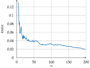
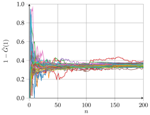
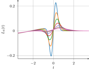
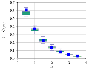
$x_{0}$	0.5	1.0	1.5	2.0	2.5	3.0	3.5
$1-G(x_{0})$	0.607	0.368	0.223	0.135	0.0821	0.0414	0.0302
Mean $1-\tilde{G}(x_{0})$	0.570	0.361	0.228	0.136	0.0976	0.0441	0.0261
St. dev.	0.028	0.025	0.021	0.015	0.0140	0.0076	0.0097

Figure 1: Results corresponding to item 1a. Top left: plot of the root mean squared error vs the number of observations $n$, averaged over 50 runs. Top right: 50 runs for $n=0$ to $n=200$, for $x_{0}=1$. Bottom left: $L_{h}$ for $h\in[0.23,0.89]$. More precisely: $h=0.025\cdot(1.25)^{q}$, with $q=10,11,\ldots,16$. Smaller $h$ corresponds to steeper bumps. Bottom right: boxplot of $50$ runs with $n=200$. The table corresponds to the boxplot.

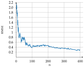
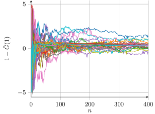
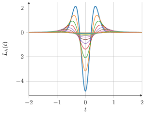
$n$	100	200	300	400
Mean	0.43	0.42	0.35	0.37
St. dev.	0.39	0.45	0.34	0.28

Figure 2: Results corresponding to Case 1b. Top left: root mean squared error vs $n$. Top right: 50 runs for $n=0$ to $n=400$, for $x_{0}=1$. Bottom left: $L_{h}$ for $h\in[0.23,0.94]$. More precisely: $h=0.05\cdot(1.15)^{q}$, with $q=10,11,\ldots,21$. Smaller $h$ corresponds to steeper bumps. Bottom right: descriptive statistics of estimator $1-\tilde{G}(1)$.

Figure 1 corresponds to Case 1a, and Figure 2 corresponds to Case 1b. In these figures (from left to right, top to bottom), we plotted the rmse as function of $n$, which is based on 50 runs of $1-\tilde{G}(1)$, the estimator of $1-G(1)=e^{-1}\approx 0.368$, which are plotted next to it. Furthermore, we plotted the kernel $L_{h}(t)$, for several values of $h$ as indicated in the captions. For Case 1, we also included a boxplot to show the performance of these 50 runs for $x_{0}$ ranging from $0.5$ to $3.5$.

From the figures we note the following. Firstly, the rmse is clearly smaller in Case 1a compared to 1b. This was to be expected because $\gamma=0$ in Case 1a, and $\gamma=1$ in Case 1b, which leads to inferior worst case minimax convergence rates in theory. Note that in Case 1b the estimators are often not even within $[0,1]$. In Case 1a we see some slight bias for smaller $x_{0}$: it appears that estimation for $x$ small in this case is relatively hard, which could be due to the fact that $G(x)$ is steeper for small $x$. The $L_{h}$ kernel in Case 1a seems quite similar to the standard Gaussian differentiation kernel that would be used in the case of constant $\lambda(\cdot)$ (when $\lambda(\cdot)\equiv\lambda_{0}$ is constant, the derivative of $\int_{0}^{t}\lambda_{0}\bar{G}(s)\operatorname{d\!}s$ equals $\lambda_{0}\bar{G}(t)$). However, there is an additional ‘bump’ that compensates for the fact that $\lambda(\cdot)$ is a cosine function, rather than a constant.

6.4 Simulation results for estimating the mean

We consider the following numerical settings.

• Take $\lambda(t)=1+\sin(t)$ and $G(x)=1-e^{-x}$, $x_{1}=-1$, $h=0.08$ (as small as possible so that the numerical inversion algorithm is still stable, with parameters $\tilde{T}=30$, $c=-1$, $b=25$.

• Let $\lambda$ be the on-off rate of Example 6 and suppose that service times are uniformly distributed on $[0,2]$, such that $\mu_{G}=1$. We take $b=25$ in estimator (14).

In Case 2a, of which the results are shown in Figure 3, we see that the kernel is approximately a delta function at $b+x_{1}=24$ (as in the constant $\lambda(\cdot)$ case), with some adjustment that takes care of the fact that the arrival rate is a sine function. The histogram shows the distribution of $\hat{\mu}_{G}$, each based on a single observation. Note that the distribution is approximately normal, with some skew to the left, with mean $1.03$ and standard deviation $0.73$. Although the standard deviation seems quite large, one must take into account that the kernel $J_{b}$ is almost zero outside of $[15,25]$. During those 10 time units there are approximately 10 arrivals. Note that the kernel $J_{b}$ in Case 2a is again quite similar to kernel $J_{b}$ in case of constant $\lambda(\cdot)$ (as in Example 5): there is a Dirac delta function at $b+x_{1}$, and in addition to that there is a wave preceding the Dirac delta function to somehow compensate for the fact that $\lambda$ is not constant.

In Case 2b we used the explicit kernels as calculated in Example 6. The bias turns out to be negligible, and the standard deviation is approximately $\frac{1}{\sqrt{n}}$ after $n$ observations.

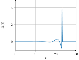
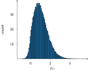
Figure 3: Results corresponding to Case 2a. On the top left we plotted the kernel $J_{b}$ and on the top right we plotted $\tilde{\mu}_{G}$ based on a single observation, for $10^{5}$ simulation runs.

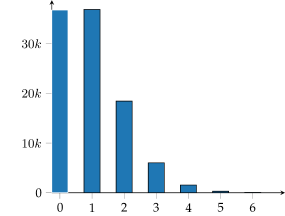
Figure 4: Results corresponding to Case 2b. We plotted the histogram of estimators based on a single observation. All estimates based on a single observation are obviously integer valued. The mean of this sample is 0.999, with a standard deviation of 0.998.

7 Proofs

7.1 Proof of Theorem 1

The proof is similar to the one of Proposition 1 in [14]. By conditioning on $\{\tau_{j},j\in{\mathbb{Z}}\}$ we obtain that

$$\mathbb{E}_{G}\exp\Big{\{}\sum_{i=1}^{m}\theta_{i}X(t_{i})\Big{\}}=\mathbb{E}_{G}\exp\Big{\{}\sum_{j\in{\mathbb{Z}}}f(\tau_{j})\Big{\}},$$

where

$$f(x)=\ln\Big{(}1+\sum_{k=1}^{m}\Big{[}e^{\sum_{i=1}^{k}\theta_{i}{\bf 1}(x\leq t_{i})}-1\Big{]}{\mathbb{P}}_{G}\{\sigma_{1}\in I_{k}(x)\}\Big{)},$$

$I_{k}(x)=(t_{k}-x,t_{k+1}-x]$, $k=1,\ldots,m-1$, and $I_{m}(x)=(t_{m}-x,\infty)$. Then Campbell’s formula yields

$$\mathbb{E}_{G}\exp\Big{\{}\sum_{j\in{\mathbb{Z}}}f(\tau_{j})\Big{\}}=\exp\Big{\{}\int_{-\infty}^{\infty}[e^{f(x)}-1]\lambda(x)\mathrm{d}x\Big{\}},$$

and our current goal is to evaluate the integral on the right hand side of the last equality. Denote this integral by $S_{m}$:

$$S_{m} \mathrel{\mathop{\mathchar 58\relax}}= \int_{-\infty}^{\infty}[e^{f(x)}-1]\lambda(x)\mathrm{d}x$$ (15)

$$= \sum_{k=1}^{m-1}\int_{-\infty}^{\infty}\big{(}\exp\big{\{}\sum_{i=1}^{k}\theta_{i}{\bf 1}(x\leq t_{i})\big{\}}-1\big{)}\big{[}\bar{G}(t_{k}-x)-\bar{G}(t_{k+1}-x)\big{]}\lambda(x)\mathrm{d}x$$

$$+\int_{-\infty}^{\infty}\big{(}\exp\big{\{}\sum_{i=1}^{m}\theta_{i}{\bf 1}(x\leq t_{i})\big{\}}-1\Big{)}\bar{G}(t_{m}-x)\lambda(x)\mathrm{d}x=\mathrel{\mathop{\mathchar 58\relax}}\sum_{k=1}^{m-1}J_{k}+L_{m}.$$

We derive (2) by iterating (15); we have

$$S_{m+1}=S_{m}+J_{m}+L_{m+1}-L_{m}=S_{1}+\sum_{k=1}^{m}[J_{k}+L_{k+1}-L_{k}].$$ (16)

For any $k\geq 1$

$$J_{k} = \Big{(}e^{\sum_{i=1}^{k}\theta_{i}}-1\Big{)}\int_{t_{k}-t_{1}}^{\infty}\big{[}\bar{G}(u)-\bar{G}(t_{k+1}-t_{k}+u)\big{]}\lambda(t_{k}-u)\mathrm{d}u$$

$$\;+\;\sum_{j=1}^{k-1}\Big{(}e^{\sum_{i=j+1}^{k}\theta_{i}}-1\Big{)}\int_{t_{k}-t_{j+1}}^{t_{k}-t_{j}}\big{[}\bar{G}(u)-\bar{G}(t_{k+1}-t_{k}+u)\big{]}\lambda(t_{k}-u)\mathrm{d}u,$$

$$L_{k} = \Big{(}e^{\sum_{i=1}^{k}\theta_{i}}-1\Big{)}\int_{t_{k}-t_{1}}^{\infty}\bar{G}(u)\lambda(t_{k}-u)\mathrm{d}u$$

$$\;+\;\sum_{j=1}^{k-1}\Big{(}e^{\sum_{i=j+1}^{k}\theta_{i}}-1\Big{)}\int_{t_{k}-t_{j+1}}^{t_{k}-t_{j}}\bar{G}(u)\lambda(t_{k}-u)\mathrm{d}u;$$

this yields

$$J_{k}-L_{k} = -\Big{(}e^{\sum_{i=1}^{k}\theta_{i}}-1\Big{)}\int_{t_{k}-t_{1}}^{\infty}\bar{G}(t_{k+1}-t_{k}+u)\lambda(t_{k}-u)\mathrm{d}u$$

$$\;-\;\sum_{j=1}^{k-1}\Big{(}e^{\sum_{i=j+1}^{k}\theta_{i}}-1\Big{)}\int_{t_{k}-t_{j+1}}^{t_{k}-t_{j}}\bar{G}(t_{k+1}-t_{k}+u)\lambda(t_{k}-u)\mathrm{d}u$$

$$= -\Big{(}e^{\sum_{i=1}^{k}\theta_{i}}-1\Big{)}\int_{t_{k+1}-t_{1}}^{\infty}\bar{G}(u)\lambda(t_{k+1}-u)\mathrm{d}u$$

$$\;-\;\sum_{j=1}^{k-1}\Big{(}e^{\sum_{i=j+1}^{k}\theta_{i}}-1\Big{)}\int_{t_{k+1}-t_{j+1}}^{t_{k+1}-t_{j}}\bar{G}(t_{k+1}-t_{k}+u)\lambda(t_{k}-u)\mathrm{d}u.$$

Then we obtain

$$J_{k}-L_{k}+L_{k+1}\;=\;\Big{(}e^{\theta_{k+1}}-1\Big{)}H(t_{k+1})+\Big{(}e^{\theta_{k+1}}-1\Big{)}\Big{(}e^{\sum_{i=1}^{k}\theta_{i}}-1\Big{)}H_{t_{k+1}-t_{1},\infty}(t_{k+1})$$

$$+\Big{(}e^{\theta_{k+1}}-1\Big{)}\sum_{j=1}^{k-1}\Big{(}e^{\sum_{i=j+1}^{k}\theta_{i}}-1\Big{)}H_{t_{k+1}-t_{j+1},t_{k+1}-t_{j}}(t_{k+1}).$$

$$\;=\;\Big{(}e^{\theta_{k+1}}-1\Big{)}\Big{[}H(t_{k+1})+\sum_{j=0}^{k-1}\Big{(}e^{\sum_{i=j+1}^{k}\theta_{i}}-1\Big{)}H_{t_{k+1}-t_{j+1},t_{k+1}-t_{j}}(t_{k+1})\Big{]},$$

where by convention we put $t_{0}=-\infty$. Taking into account that $S_{1}=(e^{\theta_{1}}-1)H(t_{1})$ and using (16) we complete the proof.

7.2 Auxiliary results

First we state two auxiliary results that are used in the subsequent proofs.

Lemma 3.

Let $\{X(t),t\geq 0\}$ be the queue–length process of the $M_{t}/G/\infty$ queue with $G\in{\mathscr{G}}(M)$, and let $R(t,\tau)\mathrel{\mathop{\mathchar 58\relax}}={\rm cov}_{G}[X(t),X(\tau)]$. Suppose that Assumption 1 holds.

• If $\sigma_{\lambda}>0$ then for any $\nu\geq 0$

  $$\int_{0}^{\infty}R(t,\tau)\mathrm{d}\tau\leq 2M\lambda_{0}e^{(\sigma_{\lambda}+\nu)t}(\sigma_{\lambda}+\nu)^{-1}.$$ (17)

• If $\sigma_{\lambda}=0$ then

  $$\int_{0}^{\infty}R(t,\tau)\mathrm{d}\tau\leq 3M\lambda_{0}(a_{1}+a_{2}t^{p}).$$

Proof.

By Corollary 1,

$$R(t,\tau)\mathrel{\mathop{\mathchar 58\relax}}={\rm cov}_{G}\big{[}X(t),X(\tau)]=\int_{\tau-t}^{\tau}\bar{G}(u)\lambda(\tau-u)\operatorname{d\!}u,\;\;\;\ \forall\tau\geq t\geq 0.$$ (18)

(a). First, assume $\sigma_{\lambda}>0$. By (4) we have for any $\nu\geq 0$

$$\int_{0}^{\infty}R(t,\tau){\bf 1}(\tau\geq t)\mathrm{d}\tau=\int_{0}^{\infty}{\bf 1}(\tau\geq t)\int_{\tau-t}^{\tau}\bar{G}(u)\lambda(\tau-u)\mathrm{d}u\mathrm{d}\tau$$

$$\leq\int_{0}^{\infty}\bar{G}(u)\mathrm{d}u\int_{0}^{t}\lambda(u)\mathrm{d}u\leq M\lambda_{0}(\sigma_{\lambda}+\nu)^{-1}e^{(\sigma_{\lambda}+\nu)t},$$ (19)

and

$$\int_{0}^{\infty}R(t,\tau){\bf 1}(\tau<t)\mathrm{d}\tau=\int_{0}^{\infty}{\bf 1}(\tau<t)\int_{t-\tau}^{t}\bar{G}(u)\lambda(t-u)\mathrm{d}u\mathrm{d}\tau\\ =\int_{0}^{t}u\bar{G}(u)\lambda(t-u)\mathrm{d}u\leq e^{(\sigma_{\lambda}+\nu)t}\int_{0}^{t}ue^{-(\sigma_{\lambda}+\nu)u}\bar{G}(u)\mathrm{d}u\leq M\lambda_{0}(\sigma_{\lambda}+\nu)^{-1}e^{(\sigma_{\lambda}+\nu)t}.$$ (20)

Summing up (19) and (20) we obtain (17).

(b). Now consider the case $\sigma_{\lambda}=0$. Using (5) and (18) we obtain

$$\int_{0}^{\infty}R(t,\tau){\bf 1}(\tau\geq t)\mathrm{d}\tau =\int_{0}^{\infty}\int_{0}^{\infty}\bar{G}(u){\bf 1}\{t\vee u\leq\tau\leq t+u\}\lambda(\tau-u)\mathrm{d}\tau\mathrm{d}u$$

$$\leq\lambda_{0}a_{1}\int_{0}^{\infty}\bar{G}(u)(t\wedge u)\mathrm{d}u+\lambda_{0}a_{2}\int_{0}^{\infty}\bar{G}(u)\int_{t\vee u}^{t+u}(\tau-u)^{p}\mathrm{d}\tau\mathrm{d}u$$

$$\leq\lambda_{0}Ma_{1}+\frac{\lambda_{0}a_{2}}{p+1}\bigg{[}\int_{0}^{t}\bar{G}(u)[t^{p+1}-(t-u)^{p+1}]\mathrm{d}u+t^{p+1}\int_{t}^{\infty}\bar{G}(u)\mathrm{d}u\bigg{]}.$$

Moreover, since $G\in{\mathscr{G}}(M)$, it holds that $t^{p+1}\int_{t}^{\infty}\bar{G}(u)\mathrm{d}u\leq Mt^{p}$ and

$$\int_{0}^{t}\bar{G}(u)[t^{p+1}-(t-u)^{p+1}]\mathrm{d}u\leq t^{p+1}\int_{0}^{t}\bar{G}(u)(p+1)\tfrac{u}{t}\mathrm{d}u\leq(p+1)Mt^{p},$$

where in the first inequality we have used that $1-[1-(u/t)]^{p}\leq(p+1)u/t$ for $0\leq u\leq t$. This yields

$$\int_{0}^{\infty}R(t,\tau){\bf 1}(\tau\geq t)\mathrm{d}\tau\leq 2M\lambda_{0}(a_{1}+a_{2}t^{p}).$$

Similarly,

$$\int_{0}^{\infty}R(t,\tau){\bf 1}(\tau<t)\mathrm{d}\tau=\int_{0}^{t}u\bar{G}(u)\lambda(t-u)\mathrm{d}u\leq M\lambda_{0}(a_{1}+a_{2}t^{p}).$$

Summing up the last two inequalities we complete the proof. ∎

Lemma 4.

Let $\delta>0$ and $p\geq 0$; then

$$\int_{T}^{\infty}e^{-\delta t}t^{p}\mathrm{d}t\leq 2\delta^{-2}T^{p-1}e^{-\delta T},$$

provided that $\delta T\geq 2p$.

Proof.

The statement is an immediate consequence of Corollary 2.5 in [6]. ∎

7.3 Proof of Theorem 2

Throughout the proof $c_{1},c_{2},\ldots$ stand for positive constants that may depend on $\beta$, $\gamma$, $k_{0}$, and $p$ only. In particular, they do not depend on $n$, $T$, and on the parameters $x_{0}$, $A$, $M$, $\sigma_{\lambda}$ and $\lambda_{0}$. The proof is divided in steps. The numbering of constants at each step of the proof starts anew, so that $c_{1},c_{2},\ldots$ are different on different appearances.

1⁰. First we show that under the premise of the theorem the estimator is well–defined. Since ${\rm supp}(K)=[0,1]$, $\widehat{K}$ is an entire function. For any $\sigma\in{\mathbb{R}}$

$$\widehat{K}(\sigma+i\omega)=\int_{0}^{1}K(t)e^{-(\sigma+i\omega)t}\mathrm{d}t,$$

and, by condition (K2), kernel $K$ is $r$ times continuously differentiable; hence repeatedly integrating by parts we obtain that for any $\omega$ and $\sigma$

$$|\widehat{K}(\sigma+i\omega)|\leq c_{1}e^{|\sigma|}(\sigma^{2}+\omega^{2})^{-r/2}.$$ (21)

In addition, in view of (K2), for any $\omega$ and $\sigma$

$$|\widehat{K}(\sigma+i\omega)|\leq c_{1}e^{|\sigma|}.$$ (22)

By Assumption  2, $\widehat{\lambda}(z)$ does not have zeros in the half–plane $\{z\in\mathbb{C}\mathrel{\mathop{\mathchar 58\relax}}{\rm Re}(z)>\sigma_{\lambda}\}$. This implies that $\widehat{K}(zh)/\widehat{\lambda}(-z)$ is an analytic function in $\{z\in\mathbb{C}\mathrel{\mathop{\mathchar 58\relax}}{\rm Re}(z)<-\sigma_{\lambda}\}$, and integration in (7) can be performed on any vertical line ${\rm Re}(z)=s$ with $s<-\sigma_{\lambda}$.

Put $s=-\sigma_{\lambda}-\delta$, where $\delta>0$ is a parameter to be specified. In the subsequent proof we assume that $\delta<1/h$ and $h<1$; this does not lead to loss of generality because $h$ will be chosen tending to zero as $n\to\infty$, and $\delta$ will always satisfy $\delta<1/h$ for large $n$. Thus, for $s=-\sigma_{\lambda}-\delta$ it follows from (7) and Assumption 2 that

$$|L_{h}(t)| \leq \frac{e^{-(\sigma_{\lambda}+\delta)t}}{2\pi}\int_{-\infty}^{\infty}\frac{|\widehat{K}((-\sigma_{\lambda}-\delta+i\omega)h)|}{|\widehat{\lambda}(\sigma_{\lambda}+\delta-i\omega)|}\mathrm{d}\omega$$

$$\leq \frac{e^{-(\sigma_{\lambda}+\delta)t}}{2\pi\lambda_{0}k_{0}}\int_{-\infty}^{\infty}|\widehat{K}((-\sigma_{\lambda}-\delta+i\omega)h)|(\delta^{2}+\omega^{2})^{\gamma/2}\mathrm{d}\omega.$$

We continue bounding this quantity:

$$|L_{h}(t)|$$

$$\leq\frac{c_{2}e^{-(\sigma_{\lambda}+\delta)t}}{\lambda_{0}}\left[\delta^{\gamma}\int_{|\omega|\leq\delta}|\widehat{K}((-\sigma_{\lambda}-\delta+i\omega)h)|\mathrm{d}\omega+\int_{|\omega|>\delta}|\widehat{K}((-\sigma_{\lambda}-\delta+i\omega)h)|\,|\omega|^{\gamma}\mathrm{d}\omega\right]$$

$$\leq\frac{c_{3}e^{-(\sigma_{\lambda}+\delta)t}}{\lambda_{0}}\left[\delta^{\gamma+1}e^{(\sigma_{\lambda}+\delta)h}+h^{-\gamma-1}\int_{|\xi|>\delta h}|\widehat{K}(-(\sigma_{\lambda}+\delta)h+i\xi)|\,|\xi|^{\gamma}\mathrm{d}\xi\right]$$

$$\leq c_{4}e^{-(\sigma_{\lambda}+\delta)(t-h)}(\lambda_{0}h^{\gamma+1})^{-1},$$ (23)

where in the first inequality above we use that $(\delta^{2}+\omega^{2})^{\gamma/2}\leq 2^{(\frac{\gamma}{2}-1)_{+}}(\delta^{\gamma}+\omega^{\gamma})$, and the last inequality follows from (21), (22) and $r>\gamma+1$.

Since $G\in\bar{{\mathscr{H}}}_{\beta,x_{0}}(A,M)$, it holds that $H(t)\leq M\lambda_{0}e^{\sigma_{\lambda}t}$ when $\sigma_{\lambda}>0$, and $H(t)\leq M\lambda_{0}(a_{1}+a_{2}t^{p})$ when $\sigma_{\lambda}=0$ [cf. (1)]. Combining this with (23) we obtain

$$\int_{0}^{\infty}|L_{h}(t-x_{0})|H(t)\mathrm{d}t\leq c_{5}\varkappa_{1}(\delta)Me^{(\sigma_{\lambda}+\delta)(x_{0}+h)}h^{-\gamma-1}<\infty,$$

where we put

$$\varkappa_{1}(\delta)\mathrel{\mathop{\mathchar 58\relax}}=\left\{\begin{array}[]{ll}\delta^{-1},&\sigma_{\lambda}>0,\\ a_{1}\delta^{-1}+a_{2}\delta^{-p-1},&\sigma_{\lambda}=0.\end{array}\right.$$

Thus the estimator $\tilde{G}_{h}(x_{0})$ is well defined, and conditions (8) of Lemma 1 hold.

2⁰. Now we establish an upper bound on the bias of $\tilde{G}_{h}(x_{0})$. By Lemma 1 and conditions (K1)–(K2) we have

$$\mathbb{E}_{G}\big{[}\tilde{G}_{h}(x_{0})\big{]} =1-\mathbb{E}_{G}\int_{0}^{T}L_{h}(t-x_{0})X(t)\mathrm{d}t=1-\int_{0}^{T}L_{h}(t-x_{0})H(t)\mathrm{d}t$$

$$=\int_{-\infty}^{\infty}\frac{1}{h}K\bigg{(}\frac{x-x_{0}}{h}\bigg{)}G(x)\mathrm{d}x+\int_{T}^{\infty}L_{h}(t-x_{0})H(t)\mathrm{d}t.$$

It follows from Taylor expansion of $G$ and (K1)-(K2) that

$$\bigg{|}\int_{-\infty}^{\infty}\frac{1}{h}K\bigg{(}\frac{x-x_{0}}{h}\bigg{)}G(x)\mathrm{d}x-G(x_{0})\bigg{|}=\bigg{|}\int_{0}^{1}K(u)[G(x_{0}+uh)-G(x_{0})]\mathrm{d}u\bigg{|}\leq C_{K}Ah^{\beta}.$$

Moreover, if $\sigma_{\lambda}>0$ then in view of (23)

$$\bigg{|}\int_{T}^{\infty}L_{h}(t-x_{0})H(t)\mathrm{d}t\bigg{|}\leq c_{1}Me^{(\sigma_{\lambda}+\delta)(x_{0}+h)}e^{-\delta T}\delta^{-1}h^{-\gamma-1}.$$

If $\sigma_{\lambda}=0$, $p>0$ and $\delta T\geq 2p$ then by Lemma 4

$$\bigg{|}\int_{T}^{\infty}L_{h}(t-x_{0})H(t)\mathrm{d}t\bigg{|}\leq c_{2}Me^{\delta(x_{0}+h)}e^{-\delta T}h^{-\gamma-1}(a_{1}\delta^{-1}+a_{2}\delta^{-2}T^{p-1}).$$

Thus,

$$\bigg{|}\int_{T}^{\infty}L_{h}(t-x_{0})H(t)\mathrm{d}t\bigg{|}\leq c_{3}\varkappa_{2}(\delta,T)Me^{(\sigma_{\lambda}+\delta)(x_{0}+h)}e^{-\delta T}h^{-\gamma-1},$$

where

$$\varkappa_{2}(\delta,T)\mathrel{\mathop{\mathchar 58\relax}}=\left\{\begin{array}[]{ll}\delta^{-1}&\sigma_{\lambda}>0\;\;\hbox{and}\;\;\sigma_{\lambda}=0,p=0,\\ a_{1}\delta^{-1}+a_{2}\delta^{-2}T^{p-1},&\sigma_{\lambda}=0,p>0.\end{array}\right.$$

Combining these inequalities we obtain

$$\Big{|}\mathbb{E}_{G}\big{[}\tilde{G}_{h}(x_{0})-G(x_{0})\big{]}\Big{|}\leq c_{4}\bigg{[}Ah^{\beta}+\varkappa_{2}(\delta,T)Me^{(\sigma_{\lambda}+\delta)(x_{0}+h)}e^{-\delta T}h^{-\gamma-1}\bigg{]}.$$ (24)

3⁰. The next step is to bound the variance of $\tilde{G}_{h}(x_{0})$. Let $R(t,\tau)\mathrel{\mathop{\mathchar 58\relax}}={\rm cov}_{G}\big{[}X(t),X(\tau)]$; then

$${\rm var}_{G}\big{[}\tilde{G}_{h}(x_{0})\big{]} = \frac{1}{n}\int_{0}^{T}\int_{0}^{T}L_{h}(t-x_{0})\overline{L_{h}(\tau-x_{0})}R(t,\tau)\mathrm{d}t\mathrm{d}\tau$$ (25)

$$\leq \frac{1}{n}\int_{0}^{T}\int_{0}^{T}|L_{h}(t-x_{0})|^{2}R(t,\tau)\mathrm{d}t\mathrm{d}\tau$$

$$\leq \frac{1}{n}\int_{0}^{\infty}|L_{h}(t-x_{0})|^{2}\int_{0}^{\infty}R(t,\tau)\operatorname{d\!}\tau\operatorname{d\!}t,$$

where the first inequality is due to Cauchy–Schwarz and symmetry of the covariance function in its arguments. Our current goal is to bound from above the expression on the right hand side of (25). We consider the cases $\sigma_{\lambda}>0$ and $\sigma_{\lambda}=0$ separately.

(a). If $\sigma_{\lambda}>0$ then using statement (a) of Lemma 3 with $\nu=\sigma_{\lambda}+2\delta$, $\delta>0$ we obtain

$${\rm var}_{G}\big{[}\tilde{G}_{h}(x_{0})\big{]} \leq \frac{\lambda_{0}M}{n(\sigma_{\lambda}+\delta)}\int_{0}^{\infty}|L_{h}(t-x_{0})|^{2}\,e^{2(\sigma_{\lambda}+\delta)t}\mathrm{d}t$$

$$\leq \frac{\lambda_{0}Me^{2(\sigma_{\lambda}+\delta)x_{0}}}{4\pi^{2}n(\sigma_{\lambda}+\delta)}\int_{-\infty}^{\infty}\bigg{|}\frac{\widehat{K}(-(\sigma_{\lambda}+\delta)h+i\omega h)}{\widehat{\lambda}(\sigma_{\lambda}+\delta-i\omega)}\bigg{|}^{2}\mathrm{d}\omega,$$

where in the last line we have used Parseval’s identity. By Assumption 2 and in view of (21) and (22)

$$\int_{-\infty}^{\infty}\bigg{|}\frac{\widehat{K}(-(\sigma_{\lambda}+\delta)h+i\omega h)}{\widehat{\lambda}(\sigma_{\lambda}+\delta-i\omega)}\bigg{|}^{2}\mathrm{d}\omega \leq\frac{1}{\lambda_{0}^{2}k_{0}^{2}}\int_{-\infty}^{\infty}|\widehat{K}(-\sigma h+i\omega h)|^{2}\big{[}\delta^{2}+\omega^{2}\big{]}^{\gamma}\mathrm{d}\omega$$

$$\leq c_{1}\lambda_{0}^{-2}e^{2\sigma h}\big{[}\delta^{2\gamma}h^{-1}+h^{-2\gamma-1}\big{]}\leq c_{2}\lambda_{0}^{-2}e^{2\sigma h}h^{-2\gamma-1},$$

where we have taken into account that $\delta<1/h$. This leads to the following bound on the variance

$${\rm var}_{G}\big{[}\tilde{G}_{h}(x_{0})\big{]}\leq c_{3}(\sigma_{\lambda}+\delta)^{-1}Me^{2(\sigma_{\lambda}+\delta)(x_{0}+h)}(\lambda_{0}nh^{2\gamma+1})^{-1}.$$ (26)

(b). Now consider the case $\sigma_{\lambda}=0$. In this case (25) and Lemma 3 show that

$${\rm var}_{G}[\tilde{G}_{h}(x_{0})]\leq\frac{c_{4}\lambda_{0}M}{n}\int_{0}^{\infty}|L_{h}(t-x_{0})|^{2}(a_{1}+a_{2}t^{p})\mathrm{d}t,$$ (27)

and our current goal is to bound the integral on the right hand side.

It follows from Assumption 1(b) that $\widehat{\lambda}(z)$ is bounded in its region of analyticity; hence the limit $\lim_{\sigma\downarrow 0}\widehat{\lambda}(\sigma+i\omega)=\widehat{\lambda}(i\omega)$ exists for almost all $\omega$ (see, e.g., [17, Chapter 19]). Moreover, Assumption 2 implies that $\widehat{\lambda}(z)$ does not vanish on the imaginary axis. Therefore $|\widehat{\lambda}(\sigma+i\omega)|^{-1}$ is finite for all $\sigma\geq 0$ and $\omega\in{\mathbb{R}}$, and function $\widehat{K}(zh)/\widehat{\lambda}(-z)$ can be analytically continued to the imaginary axis. Thus the integral in the definition (7) of $L_{h}$ can be computed over the line ${\rm Re}(z)=0$, and by Parseval’s identity and Assumption 2 we obtain

$$\int_{-\infty}^{\infty}|L_{h}(t-x_{0})|^{2}\mathrm{d}t =\frac{1}{4\pi^{2}}\int_{-\infty}^{\infty}\bigg{|}\frac{\widehat{K}(i\omega h)}{\widehat{\lambda}(-i\omega)}\bigg{|}^{2}\mathrm{d}\omega$$

$$\leq\frac{1}{4\pi^{2}}\int_{-\infty}^{\infty}|\widehat{K}(i\omega h)|^{2}|\omega|^{2\gamma}\mathrm{d}\omega\leq c_{5}h^{-2\gamma-1},$$

where the last inequality holds in view of (21), (22) and $r>\gamma+1$. Furthermore, for any real $\delta>0$

$$\int_{0}^{\infty}|L_{h}(t-x_{0})|^{2}t^{p}\mathrm{d}t$$

$$=\frac{1}{4\pi^{2}}\int_{0}^{\infty}\int_{-\infty}^{\infty}\int_{-\infty}^{\infty}\frac{\widehat{K}((-\delta+i\omega)h)}{\widehat{\lambda}(\delta-i\omega)}\overline{\frac{\widehat{K}((-\delta+i\nu)h)}{\widehat{\lambda}(\delta-i\nu)}}e^{-2\delta(t-x_{0})+i(\omega-\nu)(t-x_{0})}t^{p}\mathrm{d}\omega\mathrm{d}\nu\mathrm{d}t$$

$$=\frac{1}{4\pi^{2}}\int_{-\infty}^{\infty}\int_{-\infty}^{\infty}\frac{\widehat{K}((-\delta+i\omega)h)}{\widehat{\lambda}(\delta-i\omega)}\overline{\frac{\widehat{K}((-\delta+i\nu)h)}{\widehat{\lambda}(\delta-i\nu)}}e^{2\delta x_{0}-i(\omega-\nu)x_{0}}\frac{\Gamma(p+1)}{(2\delta+i(\nu-\omega))^{p+1}}\mathrm{d}\omega\mathrm{d}\nu$$

$$\leq\frac{\Gamma(p+1)e^{2\delta x_{0}}}{4\pi^{2}}\int_{-\infty}^{\infty}\int_{-\infty}^{\infty}\bigg{|}\frac{\widehat{K}((-\delta+i\omega)h)}{\widehat{\lambda}(\delta-i\omega)}\bigg{|}^{2}\big{[}4\delta^{2}+(\omega-\nu)^{2}\big{]}^{-\frac{1}{2}(p+1)}\mathrm{d}\omega\mathrm{d}\nu$$

$$\leq c_{6}e^{2\delta x_{0}}\delta^{-p}\int_{-\infty}^{\infty}\bigg{|}\frac{\widehat{K}((-\delta+i\omega)h)}{\widehat{\lambda}(\delta-i\omega)}\bigg{|}^{2}\mathrm{d}\omega\leq c_{7}\lambda_{0}^{-2}\delta^{-p}e^{2\delta(x_{0}+h)}h^{-2\gamma-1},$$

which together with (27) yields

$${\rm var}_{G}[\tilde{G}_{h}(x_{0})]\leq c_{8}(a_{1}+a_{2}\delta^{-p})Me^{2\delta(x_{0}+h)}(\lambda_{0}nh^{2\gamma+1})^{-1}.$$ (28)

Combining (26) and (28) we conclude that for any $\sigma_{\lambda}\geq 0$ one has

$${\rm var}_{G}[\tilde{G}_{h}(x_{0})]\leq c_{9}\varkappa_{3}(\sigma_{\lambda},\delta)Me^{2(\sigma_{\lambda}+\delta)(x_{0}+h)}\big{(}\lambda_{0}nh^{2\gamma+1}\big{)}^{-1},$$

where

$$\varkappa_{3}(\sigma_{\lambda},\delta)\mathrel{\mathop{\mathchar 58\relax}}=\left\{\begin{array}[]{ll}(\sigma_{\lambda}+\delta)^{-1},&\sigma_{\lambda}>0,\\[5.69054pt] a_{1}+a_{2}\delta^{-p},&\sigma_{\lambda}=0.\end{array}\right.$$

4⁰. Now we are in a position to finish the proof of (11). For this purpose we specify the choice of parameters $h$ and $\delta$ and substitute the corresponding expressions in the derived bounds on bias and variance.

(a). Consider first the case $\sigma_{\lambda}>0$. Here we put

$$h=h_{*}=\bigg{(}\frac{Me^{2\sigma_{\lambda}x_{0}}}{A^{2}\sigma_{\lambda}\lambda_{0}n}\bigg{)}^{1/(2\beta+2\gamma+1)},$$

and

$$\delta=\delta_{*}\mathrel{\mathop{\mathchar 58\relax}}=\frac{c_{1}}{T-x_{0}}\ln\bigg{\{}M^{\frac{\beta+\gamma}{2\beta+2\gamma+1}}(Ae^{-\sigma_{\lambda}x_{0}})^{\frac{1}{2\beta+2\gamma+1}}(\sigma_{\lambda}\lambda_{0}n)^{\frac{\beta+\gamma+1}{2\beta+2\gamma+1}}\bigg{\}}$$

with some appropriately large absolute constant $c_{1}$. Note that $\delta_{*}\to 0$ as $n\to\infty$ because $\frac{1}{T}\ln(\lambda_{0}n)\to 0$ as $n\to\infty$. With the choice of $h=h_{*}$ and $\delta=\delta_{*}$, it is straightforward to verify in (24) that the bias is bounded above by a multiple of $Ah_{*}^{\beta}$. Then substituting the expressions for $h_{*}$ and $\delta_{*}$ in (24) and (26) and taking the limit as $n\to\infty$ we obtain (11) for the case $\sigma_{\lambda}>0$.

(b). Now, let $\sigma_{\lambda}=0$ and assume first that $p=0$, i.e., the intensity function $\lambda(t)$ is bounded. Here we choose

$$h=h_{*}=\bigg{(}\frac{M}{A^{2}\lambda_{0}n}\bigg{)}^{1/(2\beta+2\gamma+1)}$$

and

$$\delta=\delta_{*}=\frac{c_{2}}{T-x_{0}}\ln\bigg{\{}M^{\frac{\beta+\gamma}{2\beta+2\gamma+1}}A^{\frac{1}{2\beta+2\gamma+1}}(\lambda_{0}n)^{\frac{\beta+\gamma+1}{2\beta+2\gamma+1}}\bigg{\}}$$

with appropriate constant $c_{2}$. Substituting these values in (24) and (28) we obtain (11).

If $p>0$ then we set

$$h=h_{*}\mathrel{\mathop{\mathchar 58\relax}}=\bigg{[}\frac{M(a_{1}+a_{2}x_{0}^{p})}{A^{2}\lambda_{0}n}\bigg{]}^{1/(2\beta+2\gamma+1)},$$

and $\delta=\delta_{*}\mathrel{\mathop{\mathchar 58\relax}}=\frac{p}{2x_{0}}$. It is easily checked that under this choice (11) holds with

$$\varphi_{n}=A^{(2\gamma+1)/(2\beta+2\gamma+1)}\bigg{[}\frac{M(a_{1}+a_{2}x_{0}^{p})}{\lambda_{0}n}\bigg{]}^{\beta/(2\beta+2\gamma+1)}.$$

7.4 Proof of Theorems 3 and 4

We provide a unified proof of Theorems 3 and 4. Each step of the proof considers two cases: $\sigma_{\lambda}>0$ (corresponds to the proof of Theorem 3) and $\sigma_{\lambda}=0$ (corresponds to the proof of Theorem 4).

Throughout the proof $c_{1},c_{2},\ldots$ stand for constants depending on $\gamma$, $k_{0}$ and $p$ only. In particular, they do not depend on $M$, $\lambda_{0}$ and $\sigma_{\lambda}$. In order to avoid additional technicalities in the sequel we assume that $\gamma$ is integer.

1⁰. First we bound the bias of $\tilde{\mu}_{G}$. By Lemma 2

$$\mathbb{E}_{G}[\tilde{\mu}_{G}]=\int_{0}^{T}J_{b}(t)H(t)\mathrm{d}t=\int_{0}^{\infty}\psi_{b}(x)\bar{G}(x)\mathrm{d}x-\int_{T}^{\infty}J_{b}(t)H(t)\mathrm{d}t.$$

Therefore

$$\big{|}\mathbb{E}_{G}[\tilde{\mu}_{G}]-\mu_{G}\big{|}\leq\int_{b}^{\infty}\bar{G}(x)\mathrm{d}x+\int_{T}^{\infty}|J_{b}(t)|H(t)\mathrm{d}t.$$ (29)

Since $G\in{\mathscr{G}}(M)$,

$$\int_{b}^{\infty}\bar{G}(x)\mathrm{d}x\leq\int_{b}^{\infty}\frac{x}{b}\bar{G}(x)\mathrm{d}x\leq Mb^{-1}.$$ (30)

Our current goal is to bound the second integral on the right hand side of (29).

Let $s=-\sigma$, where $\sigma\mathrel{\mathop{\mathchar 58\relax}}=\sigma_{\lambda}+\delta$ with some parameter $\delta>0$ to be specified. By definition of $J_{b}(t)$ and by Assumption 2

$$|J_{b}(t)| \leq \frac{e^{-\sigma t}}{2\pi\lambda_{0}k_{0}}\int_{-\infty}^{\infty}|\widehat{\psi}_{b}(-\sigma+i\omega)|\big{[}(\sigma-\sigma_{\lambda})^{2}+\omega^{2}\big{]}^{\gamma/2}\mathrm{d}\omega$$

$$\leq c_{1}e^{-\sigma t}\lambda_{0}^{-1}\bigg{\{}\delta^{\gamma}\int_{-\infty}^{\infty}|\widehat{\psi}_{b}(-\sigma+i\omega)|\mathrm{d}\omega+\int_{-\infty}^{\infty}|\widehat{\psi}_{b}(-\sigma+i\omega)|\cdot|\omega|^{\gamma}\mathrm{d}\omega\bigg{\}}.$$

Repeatedly integrating by parts the integral $\int_{-1/4}^{b+1/4}\psi_{b}(t)e^{(\sigma-i\omega)t}\mathrm{d}t$ we obtain for any $r=1,2,\ldots$ that

$$|\widehat{\psi}_{b}(-\sigma+i\omega)|\leq c_{2}(r)e^{\sigma(b+1/4)}(\sigma^{2}+\omega^{2})^{-r/2},$$

where constant $c_{2}(r)$ depends on $r$. This inequality with $r>1$ yields

$$\int_{-\infty}^{\infty}|\widehat{\psi}_{b}(-\sigma+i\omega)|\mathrm{d}\omega \leq c_{3}(r)e^{\sigma(b+1/4)}\sigma^{-r+1}$$

and with $r>\gamma+1$

$$\int_{-\infty}^{\infty}|\widehat{\psi}_{b}(-\sigma+i\omega)|\cdot|\omega|^{\gamma}\mathrm{d}\omega\leq c_{4}(r)e^{\sigma(b+1/4)}\sigma^{-r+\gamma+1}.$$

Therefore the following bound holds

$$|J_{b}(t)|\leq c_{5}(r)\lambda_{0}^{-1}e^{-\sigma(t-b-1/4)}\Big{\{}\delta^{\gamma}\sigma^{-r+1}+\sigma^{-r+\gamma+1}\Big{\}},$$

where $r>\gamma+1$.

(a). First, consider the case $\sigma_{\lambda}>0$. By Assumption 1(a), $H(t)\leq M\lambda_{0}e^{\sigma_{\lambda}t}$; hence

$$\int_{T}^{\infty}|J_{b}(t)|H(t)\mathrm{d}t\leq\frac{c_{5}(r)M}{\sigma^{r-1}\delta}(\delta^{\gamma}+\sigma^{\gamma})e^{\sigma(b+1/4)}e^{-\delta T}.$$ (31)

Combining (31), (30) and (29) we obtain

$$\big{|}\mathbb{E}_{G}[\tilde{\mu}_{G}]-\mu_{G}\big{|}\leq Mb^{-1}+c_{5}(r)M\delta^{-1}(\sigma_{\lambda}+\delta)^{-r+\gamma+1}e^{(\sigma_{\lambda}+\delta)(b+1/4)}e^{-\delta T}.$$

In particular, if we set $r=\gamma+2$ and if

$$T-b-\tfrac{1}{4}\geq\frac{1}{\delta}\ln\bigg{(}\frac{be^{\sigma_{\lambda}(b+1/4)}}{\sigma_{\lambda}}\bigg{)}$$ (32)

then

$$\big{|}\mathbb{E}_{G}[\hat{\mu}_{G}]-\mu_{G}\big{|}\leq c_{6}Mb^{-1}.$$ (33)

(b). Now let $\sigma_{\lambda}=0$. In view of Assumption 1(b), $H(t)\leq M\lambda_{0}(a_{1}+a_{2}t^{p})$ so that

$$\int_{T}^{\infty}|J_{b}(t)|H(t)\mathrm{d}t\leq c_{5}(r)\delta^{\gamma-r+1}Me^{\delta(b+1/4)}\bigg{[}a_{1}\delta^{-1}e^{-\delta T}+a_{2}\int_{T}^{\infty}t^{p}e^{-\delta t}\mathrm{d}t\bigg{]}.$$

If $\delta T\geq 2p$ then using Lemma 4 we obtain

$$\int_{T}^{\infty}|J_{b}(t)|H(t)\mathrm{d}t\leq c_{7}(r)\delta^{\gamma-r}Me^{-\delta(T-b-1/4)}\big{(}a_{1}+a_{2}\delta^{-1}T^{p-1}\big{)}.$$ (34)

It follows from (34) that if

$$T-b-\frac{1}{4}\geq\frac{1}{\delta}\ln\Big{\{}b\delta^{\gamma-r}(a_{1}+a_{2}\delta^{-1}T^{p-1})\Big{\}},\;\;T\geq\frac{2p}{\delta}$$ (35)

then again (33) holds.

We conclude that the bound (33) on the bias holds, provided that $b$ and $\delta$ are chosen to satisfy (32) in case $\sigma_{\lambda}>0$ and (35) in case $\sigma_{\lambda}=0$.

2⁰. Now we proceed with bounding the variance of $\tilde{\mu}_{G}$. We have

$${\rm var}_{G}[\tilde{\mu}_{G}]=\frac{1}{n}\int_{0}^{T}\int_{0}^{T}J_{b}(t)\overline{J_{b}(\tau)}R(t,\tau)\mathrm{d}t\mathrm{d}\tau\leq\frac{1}{n}\int_{0}^{\infty}|J_{b}(t)|^{2}\int_{0}^{\infty}R(t,\tau)\mathrm{d}\tau\mathrm{d}t,$$ (36)

where $R(t,\tau)={\rm cov}_{G}[X(t),X(\tau)]$ is given in (18).

(a). Let $\sigma_{\lambda}>0$; then, applying Lemma 3(a) with $\nu=\sigma_{\lambda}+2\delta$ we have

$${\rm var}_{G}[\tilde{\mu}_{G}] \leq \frac{M\lambda_{0}}{n(\sigma_{\lambda}+\delta)}\int_{0}^{\infty}|J_{b}(t)|^{2}e^{2(\sigma_{\lambda}+\delta)}\mathrm{d}t$$ (37)

$$\leq \frac{M\lambda_{0}}{4\pi^{2}n(\sigma_{\lambda}+\delta)}\int_{-\infty}^{\infty}\bigg{|}\frac{\widehat{\psi}_{b}(-\sigma_{\lambda}-\delta+i\omega)}{\widehat{\lambda}(\sigma_{\lambda}+\delta-i\omega)}\bigg{|}^{2}\mathrm{d}\omega.$$

We recall that, by Assumption 2, for $\sigma=\sigma_{\lambda}+\delta$, $\delta>0$ one has

$$\int_{-\infty}^{\infty}\bigg{|}\frac{\widehat{\psi}_{b}(-\sigma+i\omega)}{\widehat{\lambda}(\sigma-i\omega)}\bigg{|}^{2}\mathrm{d}\omega\leq\frac{1}{\lambda_{0}^{2}k_{0}^{2}}\int_{-\infty}^{\infty}|\widehat{\psi}_{b}(-\sigma+i\omega)|^{2}[\delta^{2}+\omega^{2}]^{\gamma}\mathrm{d}\omega,$$

and the integral on the right hand side is bounded as follows. First, by Parseval’s identity,

$$\int_{-\infty}^{\infty}|\widehat{\psi}_{b}(-\sigma+i\omega)|^{2}\mathrm{d}\omega=2\pi\int_{-1/4}^{b+1/4}e^{2\sigma t}\psi_{b}^{2}(t)\mathrm{d}t\leq\pi e^{2\sigma(b+1/4)}\sigma^{-1}.$$ (38)

Second, for integer $\gamma\geq 0$ we have

$$\int_{-\infty}^{\infty}|\widehat{\psi}_{b}(-\sigma+i\omega)|^{2}|\omega|^{2\gamma}\mathrm{d}\omega=2\pi\int_{-1/4}^{b+1/4}\bigg{|}\frac{\mathrm{d}^{\gamma}}{\mathrm{d}t^{\gamma}}[e^{\sigma t}\psi_{b}(t)]\bigg{|}^{2}\mathrm{d}t\\ =2\pi\int_{-1/4}^{b+1/4}\bigg{|}\sum_{j=0}^{\gamma}\tbinom{\gamma}{j}\sigma^{j}e^{\sigma t}\psi^{(\gamma-j)}_{b}(t)\bigg{|}^{2}\mathrm{d}t\leq c_{1}\sum_{j=0}^{\gamma}\sigma^{2j}\int_{-1/4}^{b+1/4}e^{2\sigma t}|\psi^{(\gamma-j)}_{b}(t)|^{2}\mathrm{d}t.$$

By construction, derivatives of $\psi_{b}$ are nonzero only on the intervals $[-1/4,0]$ and $[b,b+1/4]$; therefore

$$\int_{-\infty}^{\infty}|\widehat{\psi}_{b}(-\sigma+i\omega)|^{2}|\omega|^{2\gamma}\mathrm{d}\omega\leq c_{2}e^{2\sigma(b+1/4)}\Big{[}\sigma^{2\gamma}(b+\tfrac{1}{2})+\sum_{j=0}^{\gamma-1}\sigma^{2j}\Big{]}.$$ (39)

Combining (38) and (39) we obtain

$$\int_{-\infty}^{\infty}\bigg{|}\frac{\widehat{\psi}_{b}(-\sigma+i\omega)}{\widehat{\lambda}(\sigma-i\omega)}\bigg{|}^{2}\mathrm{d}\omega\leq c_{3}\lambda_{0}^{-2}e^{2\sigma(b+1/4)}\bigg{(}\delta^{2\gamma}\sigma^{-1}+\sigma^{2\gamma}(b+\tfrac{1}{2})+\sum_{j=0}^{\gamma-1}\sigma^{2j}\bigg{)}$$

which along with (37) yields

$${\rm var}_{G}[\tilde{\mu}_{G}]\leq\frac{c_{4}Me^{2(\sigma_{\lambda}+\delta)(b+1/4)}}{\lambda_{0}n(\sigma_{\lambda}+\delta)}\bigg{[}\frac{\delta^{2\gamma}}{\sigma_{\lambda}+\delta}+(\sigma_{\lambda}+\delta)^{2\gamma}(b+\tfrac{1}{2})+\sum_{j=0}^{\gamma-1}(\sigma_{\lambda}+\delta)^{2j}\bigg{]}.$$

We set

$$\delta=\delta_{*}\mathrel{\mathop{\mathchar 58\relax}}=\frac{1}{b};$$

also $b$ will be always chosen so that $b\geq\sigma_{\lambda}^{-1}$ for large $n$. Under these conditions we finally obtain

$${\rm var}_{G}[\tilde{\mu}_{G}]\leq c_{5}M\sigma_{\lambda}^{2\gamma-1}be^{2\sigma_{\lambda}(b+1/4)}(\lambda_{0}n)^{-1}.$$

We note also that with the choice $\delta=\delta_{*}$ the bound on the bias (33) holds provided that

$$T\geq b+b\sigma_{\lambda}(b+1/4)+b\ln(b/\sigma_{\lambda});$$

see (32).

(b). Now consider the case $\sigma_{\lambda}=0$. It follows from (36) and Lemma 3 that

$${\rm var}_{G}[\tilde{\mu}_{G}]\leq\frac{c_{6}M\lambda_{0}}{n}\int_{0}^{T}|J_{b}(t)|^{2}(a_{1}+a_{2}t^{p})\mathrm{d}t.$$

Since $|\widehat{\lambda}(\sigma+i\omega)|^{-1}$ is finite for all $\sigma\geq 0$ and $\omega\in{\mathbb{R}}$, function $\widehat{\psi}_{b}(z)/\widehat{\lambda}(-z)$ can be analytically continued to the imaginary axis. Therefore, by Parseval’s identity and Assumption 2 we obtain

$$\int_{-\infty}^{\infty}|J_{b}(t)|^{2}\mathrm{d}t =\frac{1}{4\pi^{2}}\int_{-\infty}^{\infty}\bigg{|}\frac{\widehat{\psi}_{b}(i\omega)}{\widehat{\lambda}(-i\omega)}\bigg{|}^{2}\mathrm{d}\omega\leq\frac{1}{4\pi^{2}\lambda_{0}^{2}k_{0}^{2}}\int_{-\infty}^{\infty}|\widehat{\psi}_{b}(i\omega)|^{2}|\omega|^{2\gamma}\mathrm{d}\omega$$

$$\leq c_{7}\lambda_{0}^{-2}\int_{-1/4}^{b+1/4}|\psi_{b}^{(\gamma)}(t)|^{2}\mathrm{d}t\leq c_{8}\lambda_{0}^{-2},$$

and for $\delta>0$

$$\int_{0}^{\infty}|J_{b}(t)|^{2}t^{p+1}\mathrm{d}t =\frac{1}{4\pi^{2}}\int_{0}^{\infty}\int_{-\infty}^{\infty}\int_{-\infty}^{\infty}\frac{\widehat{\psi}_{b}(-\delta+i\omega)}{\widehat{\lambda}(\delta-i\omega)}\overline{\frac{\widehat{\psi}_{b}(-\delta+i\nu)}{\widehat{\lambda}(\delta-i\nu)}}e^{-2\delta t+i(\omega-\nu)t}t^{p}\mathrm{d}\omega\mathrm{d}\nu\mathrm{d}t$$

$$=\frac{1}{4\pi^{2}}\int_{-\infty}^{\infty}\int_{-\infty}^{\infty}\frac{\widehat{\psi}_{b}(-\delta+i\omega)}{\widehat{\lambda}(\delta-i\omega)}\overline{\frac{\widehat{\psi}_{b}(-\delta+i\nu)}{\widehat{\lambda}(\delta-i\nu)}}\frac{\Gamma(p+1)}{(2\delta+i(\nu-\omega))^{p+1}}\mathrm{d}\omega\mathrm{d}\nu$$

$$\leq\frac{\Gamma(p+1)}{4\pi^{2}}\int_{-\infty}^{\infty}\int_{-\infty}^{\infty}\bigg{|}\frac{\widehat{\psi}_{b}(-\delta+i\omega)}{\widehat{\lambda}(\delta-i\omega)}\bigg{|}^{2}\big{[}4\delta^{2}+(\omega-\nu)^{2}\big{]}^{-\frac{1}{2}(p+1)}\mathrm{d}\omega\mathrm{d}\nu$$

$$\leq\frac{c_{9}}{\delta^{p}}\int_{-\infty}^{\infty}\bigg{|}\frac{\widehat{\psi}_{b}(-\delta+i\omega)}{\widehat{\lambda}(\delta-i\omega)}\bigg{|}^{2}\mathrm{d}\omega.$$

Therefore

$${\rm var}_{G}[\tilde{\mu}_{G}]\leq c_{10}\frac{M\lambda_{0}}{n}(a_{1}+a_{2}\delta^{-p})\int_{-\infty}^{\infty}\bigg{|}\frac{\widehat{\psi}_{b}(-\delta+i\omega)}{\widehat{\lambda}(\delta-i\omega)}\bigg{|}^{2}\mathrm{d}\omega.$$

Using the same reasoning as before

$$\int_{-\infty}^{\infty}\bigg{|}\frac{\widehat{\psi}_{b}(-\delta+i\omega)}{\widehat{\lambda}(\delta-i\omega)}\bigg{|}^{2}\mathrm{d}\omega\leq c_{11}\lambda_{0}^{-2}e^{2\delta(b+1/4)}\Big{[}\delta^{2\gamma}(b+\tfrac{1}{2})+\sum_{j=0}^{\gamma-1}\delta^{2j}+\delta^{2\gamma-1}\Big{]}.$$

We again set $\delta=\delta_{*}\mathrel{\mathop{\mathchar 58\relax}}=b^{-1}$; with this choice

$${\rm var}_{G}[\tilde{\mu}_{G}]\leq c_{12}M(a_{1}+a_{2}b^{p})(\lambda_{0}n)^{-1},$$

and the bound on the bias is given in (33) provided that

$$T\geq b+\frac{1}{4}+b\ln b+b\ln(a_{1}+a_{2}bT^{p-1}),\;\;T\geq 2p\ln b;$$

see (35).

3⁰. Now we complete the proof by selecting $b$ to balance the obtained bounds on the bias and variance.

(a). Consider the case $\sigma_{\lambda}>0$. Let

$$b=b_{*}=\frac{1}{2\sigma_{\lambda}}\bigg{\{}\ln\bigg{(}\frac{M\lambda_{0}n}{\sigma_{\lambda}^{2\gamma-1}}\bigg{)}-3\ln\bigg{[}\frac{1}{2\sigma_{\lambda}}\ln\bigg{(}\frac{M\lambda_{0}n}{\sigma_{\lambda}^{2\gamma-1}}\bigg{)}\bigg{]}\bigg{\}}-\frac{1}{4}.$$

We note that because $[\ln(\lambda_{0}n)]^{2}/T\to 0$ as $n\to\infty$, (32) is fulfilled for large $n$ with $b=b_{*}$ and $\delta=\delta_{*}=1/b_{*}$. Therefore substituting the expression for $b_{*}$ in the bounds for the bias and variance we obtain

$$\limsup_{n\to\infty}\Big{\{}\varphi_{n}^{-1}{\cal R}[\tilde{\mu}_{G};{\mathscr{G}}(M)\big{]}\Big{\}}\leq C_{1},\;\;\;\varphi_{n}\mathrel{\mathop{\mathchar 58\relax}}=M\sigma_{\lambda}\ln\bigg{(}\frac{M\lambda_{0}n}{\sigma_{\lambda}^{2\gamma-1}}\bigg{)}.$$

(b). Now, let $\sigma_{\lambda}=0$, assume that $a_{2}=0$. In this case the bound on the variance is ${\rm var}_{G}[\tilde{\mu}_{G}]\leq c_{1}M(\lambda_{0}n)^{-1}$ and on the bias $Mb^{-1}$. If we choose $b\geq b_{*}\geq c_{2}\sqrt{M\lambda_{0}n}$ with appropriate absolute constant $c_{2}$ then under condition $\sqrt{\lambda_{0}n}\ln(\lambda_{0}n)/T\to 0$ as $n\to\infty$ we obtain that

$$\limsup_{n\to\infty}\bigg{\{}\sqrt{\frac{\lambda_{0}n}{M}}\,{\cal R}[\tilde{\mu}_{G};{\mathscr{G}}(M)]\bigg{\}}\leq C_{2}.$$

If $a_{2}>0$ then we set $b=b_{*}=\big{[}M\lambda_{0}n\big{]}^{1/(p+2)}$. If $\frac{1}{T}(\lambda_{0}n)^{1/(p+2)}\ln(\lambda_{0}n)\to 0$ as $n\to\infty$ then (35) is fulfilled for large $n$ and

$$\varphi_{n}\mathrel{\mathop{\mathchar 58\relax}}=M^{(p+1)/(p+2)}(\lambda_{0}n)^{-1/(p+2)}.$$

References

- [1] Abramovich, F., Pensky, M., and Rozenholc, Y. Laplace deconvolution with noisy observations. Electron. J. Stat. 7 (2013), 1094–1128.
- [2] Antunes, N., Pipiras, V., and Veitch, D. Skampling for the flow duration distribution. Proceedings of 29th International Teletraffic Congress (ITC 29) 1 (2017), 63–71.
- [3] Baccelli, F., Kauffman, B., and Veitch, D. Inverse problems in queueing theory and internet probing. Queueing Syst. 63 (2009), 59–107.
- [4] Bigot, J., Gadat, S., Klein, T., and Marteau, C. Intensity estimation of non-homogeneous Poisson processes from shifted trajectories. Electron. J. Stat. 7 (2013), 881–931.
- [5] Bingham, N. H., and Pitts, S. M. Non–parametric estimation for the queue. Ann. Inst. Statist. Math. 51 (1999), 71–97.
- [6] Borwein, J. M., and O-Yeat, C. Uniform bounds for the complementary incomplete gamma function. Math. Inequal. Appl. 12 (2009), 115 – 121.
- [7] Brown, M. An estimation problem. Ann. Math. Statist. 41 (1970), 651 – 654.
- [8] Coifman, B., and Cassidy, M. Vehicle reidentification and travel time measurement on congested freeways. Transportation Research Part A: Policy and Practice 36, 10 (2002), 899 – 917.
- [9] Dobrzyński, M., and Bruggeman, F. J. Elongation dynamics shape bursty transcription and translation. Proceedings of the National Academy of Sciences 106, 8 (2009), 2583–2588.
- [10] Doetsch, G. Introduction to the Theory and Application of the Laplace Transformation. Springer-Verlag, Berlin, 1974.
- [11] Durbin, F. Numerical inversion of Laplace transforms: an efficient improvement to Dubner and Abate’s method. Comput. J. 17, 4 (1973), 371–376.
- [12] Eick, S., Massey, W., and Whitt, W. The physics of the queue. Management Science 39, 2 (1993), 241–252.
- [13] Fan, J. On the optimal rates of convergence for nonparametric deconvolution problems. Ann. Statist. 19, 3 (1991), 1257–1272.
- [14] Goldenshluger, A. Nonparametric estimation of the service time distribution in the queue. Adv. in Appl. Probab. 48, 4 (2016), 1117–1138.
- [15] Goldenshluger, A. The estimation problem revisited. Bernoulli 24 (2018), 2531–2568.
- [16] Goldenshluger, A., and Nemirovski, A. On spatially adaptive estimation of nonparametric regression. Math. Methods Statist. 6, 2 (1997), 135–170.
- [17] Hille, E. Analytic Function Theory, vol. II. American Mathematical Society Chelsey Publishing, Providence, RI., 1962.
- [18] Jansen, H. M., Mandjes, M. R. H., De Turck, K., and Wittevrongel, S. A large deviations principle for infinite-server queues in a random environment. Queueing Systems 82, 1 (Feb 2016), 199–235.
- [19] Krishnamurthy, V., and Elliot, R. Filters for estimating Markov modulated Poisson processes and image-based tracking. Automatica 33, 5 (1997), 821 – 833.
- [20] Kutoyants, Y. A. Statistical Inference for Spatial Poisson Processes, vol. 134 of Lecture Notes in Statistics. Springer-Verlag, New York, 1998.
- [21] Lepskiĭ, O. V. A problem of adaptive estimation in Gaussian white noise. Teor. Veroyatnost. i Primenen. 35, 3 (1990), 459–470.
- [22] Schweer, S., and Wichelhaus, C. Nonparametric estimation of the service time distribution in the discrete-time queue with partial information. Stoch. Process. Appl. 125 (2015), 233 – 253.
- [23] Tsybakov, A. B. Introduction to Nonparametric Estimation. Springer Series in Statistics. Springer, New York, 2009.
- [24] Widder, D. The Laplace Transform. Princeton University Press, Princeton, 1946.
- [25] Zhang, C.-H. Fourier methods for estimating mixing densities and distributions. Ann. Statist. 18, 2 (1990), 806–831.