An Efficient Monte Carlo Algorithm for Determining the Minimum Energy Structures of Metallic Grain Boundaries

Abstract

Sampling minimum energy grain boundary (GB) structures in the five-dimensional crystallographic phase space can provide much-needed insight into how GB crystallography affects various interfacial properties. However, the complexity and number of parameters involved often limits the extent of this exploration to a small set of interfaces. In this article, we present a fast Monte Carlo scheme for generating zero-Kelvin, low energy GB structures in the five-dimensional crystallographic phase space. The Monte Carlo trial moves include removal and insertion of atoms in the GB region, which create a diverse set of GB configurations and result in a rapid convergence to the low energy structure. We have validated the robustness of this approach by simulating over 1184 tilt, twist, and mixed character GBs in both fcc (Aluminum and Nickel) and bcc ($\alpha$-Iron) metallic systems.

Introduction

Grain boundaries (GBs) influence a wide array of mechanical [lehockey1997creep, lehockey1998improving, chen2000role, bechtle2009grain, kobayashi2010grain, gertsman2001study, king2008observations], chemical [mishin1999grain, chen2007percolation, fujita2004using] and functional [babcock1995nature, frary2003nonrandom] properties in polycrystalline materials. However, they are also among the least understood defect types due to the vast and topologically complex five-dimensional (5-D) crystallographic phase-space of interfaces [patala2013symmetries, patala2012improved]. In other words, the GB properties are functions of, at the least, five macroscopic crystallographic degrees of freedom (DOF).

In general, for single component metallic systems, there exist nine crystallographic parameters that uniquely define the structure of a GB [kalonji1982symmetry]. These parameters are classified into macroscopic and microscopic DOF—five parameters specifying the misorientation and boundary plane orientation and the additional four representing the microscopic relative displacements between the adjoining lattices and the translation of the boundary plane along its normal vector. However, under conditions of thermodynamic equilibrium, it is generally accepted that the five macroscopic DOF are sufficient for representing the properties of interfaces [lejcek2010grain].

For developing reliable GB structure-property relationships, the lowest energy GB structures, computed at $0\text{\,}\mathrm{K}$, are essential. The energy landscape and the structure of a GB with fixed crystallography (the five macroscopic parameters) depends on the microscopic DOF and the atomic density $\lambda$ [hickman2017extra] (traditionally controlled by tuning the allowed extent of overlap between atoms). In the past few decades, several, reasonably successful efforts have been made to predict the low-energy GB structures [rittner1996simulations, tschopp2007structures, tschopp2007structural, olmsted2009survey, erwin2012continuously, banadaki2016simple]. While the implementation varies slightly, these techniques generally rely on generating a large number of initial GB configurations by varying the microscopic DOF of an interface, which can be considered as a brute-force approach for determining the minima in the energy landscape. While such a brute-force approach might suffice for simulating GBs with low $\Sigma$-number [grimmer1976coincidence], the computational cost usually increases as the symmetry of the GB is reduced.

Monte Carlo (MC) based algorithms have been routinely utilized for finding minima in energy landscapes in a variety of complex systems in condensed-matter physics [landau2014guide]. However, such a technique has never been applied to computing the minimum energy structures for GBs in single component systems. This is primarily due to the fact that atoms along the interface are not constrained to lie on a fixed lattice [landau2014guide]. For example, hybrid Monte-Carlo/Molecular-Dynamics simulations have been utilized to compute low energy GB structures in binary alloy systems [pan2016effect, pan2017formation]. These alloys have at least two components and the trial moves correspond to swapping the positions of unlike atoms. Unfortunately, in single component systems, atom swapping does not change the configuration of the bicrystal. In this article, we introduce a Monte Carlo based GB energy minimization algorithm applicable for single component systems. The advantage of a MC framework is that, when the acceptance probabilities are devised appropriately [newman1999monte], it can be utilized to compute thermodynamic equilibrium properties in a variety of relevant statistical ensembles.

As will be discussed in the next section, the trial perturbations that facilitate the MC-based approach involve both atom removal and, more importantly, atom insertions in the GB region. These two Monte-Carlo moves change the density of the GBs and are likely the most important perturbations for sampling the energy landscape of the microscopic DOF of an interface. There have been recent studies where atom removal and insertions were utilized to compute minimum energy structures or to investigate phase transitions in GB structures. For example, in [frolov2013structural], the atomic density was allowed to vary by removing periodic boundary conditions in the GB plane. The free surfaces act as sources and sinks for atoms. This facilitated the required changes in grain boundary density and a structural phase transition was observed. In [zhu2018predicting] and [frolov2018grain], low energy GB structures were obtained using a genetic algorithm where, among others, atom removal and insertion were used to perturb the GB structure. The insertions were made by constructing a uniform grid in the GB region and filling the unoccupied grid points at random.

For a Monte-Carlo simulation to work in an efficient manner, it is important that the increase in energy due to the perturbations are not always too large. However, if atoms are inserted randomly, the Monte-Carlo simulations will take a long time to converge due to low acceptance rates. In this article, we introduce a geometric construction to identify voids for atom insertion in the GB region, which alleviates the large increases in energy. This technique is similar to the cavity based MC method developed for the simulation of dense fluids [mezei1980cavity]. Inserting atoms in these voids and minimizing the structure dramatically improves the acceptance probability of the atom-insertion move. As far as the authors are aware, there has been only one previous report that utilized atom insertions and removals in a Monte-Carlo framework for defects in crystalline systems. Phillpot and Rickman [phillpot1992simulated] proposed a grand canonical framework, where sites with fractional occupancies instead of atoms are used, to obtain ground state structures in the presence of defects. In [phillpot1992simulated], a simple Lennard-Jones potential is used to compute the minimum energy structure of $(110)$ twist GB. However, in this technique, the sites for insertion are determined a priori and are fixed during the MC simulation. Our algorithm builds on these ideas and shows that low-energy configurations for GBs can be obtained for a diverse set of GB crystallographic characters in both fcc (Aluminum and Nickel) and bcc ($\alpha$-Iron) metallic systems.

The MC approach, introduced in this article, is also very efficient in generating the low energy GB structures. The biggest obstacle for generating large GB databases that are well-sampled in the 5-D crystallographic phase-space is the massive number of simulations required to obtain the lowest-energy GB structure. For example, determining the lowest energy structure for a typical GB using such brute force algorithms requires anywhere between $1000$ to $150\,000$ unique energy-minimization simulations. In this article, we also show that the proposed Monte Carlo scheme is more efficient in generating the low-energy GB structures when compared to such traditional brute-force simulations. In the following sections, we describe the Monte Carlo algorithm, the trial moves and the test cases, involving the three GB databases, in greater detail.

Methodology

Our Monte Carlo algorithm starts with an initial GB configuration and applies random perturbations (trial moves), which are then evaluated using a Metropolis-like criterion [allen1989computer]: accepted if the energy is reduced, accepted or rejected by a Boltzmann-weighted probability if the energy increases. At each step of the simulation, the following perturbations may be introduced: (a) removal of an atom from the GB and (b) insertion of an atom in the GB region.

The trial move involving atom removal (or creation of a vacancy) is inspired by investigations of von Alfthan et al. [von2006structures], Yu and Demkowicz [yu2015non], and Tschopp et al. [tschopp2014binding]. Initially, we only considered trial moves involving atom removal and realized that applying just this perturbation does not result in the low-energy structure in many of the test cases (described in the later part of the article). We observed that an efficient convergence to the low energy GB structure is obtained by also considering perturbations that involve atom insertions at GB interstitial sites.

The algorithm starts with an initial random GB configuration, which is created using a random set of microscopic DOF for the interface. The next step involves choosing one of the two trial moves stochastically (i.e., the removal and insertion moves are chosen with a probability of $p_{\text{rm}}$ and $p_{\text{in}}=1-p_{\text{rm}}$, respectively). Once the decision for removal or insertion has been made, the atom to remove or the interstitial site for atom insertion is also chosen stochastically to facilitate the possibility of generating a diverse set of GB structures. For example, to determine the GB atom to remove , we first assign a removal probability $p_{rm,i}$, for each atom $i$ in the GB, which is given by:

$$p_{\text{rm},i}=\begin{cases}\left(E_{i}-E_{\circ}\right)/\left(\sum_{j=1}^{N_{\text{GB}}}(E_{j}-E_{\circ})\right),&\text{if }E_{i}\geq E_{\circ}\\ 0,&\text{otherwise}\end{cases}$$ (1)

where $E_{i}$ is the energy of the $i^{\text{th}}$ GB atom, $E_{\circ}$ is the cohesive energy of the atom in the single crystal configuration at $0\text{\,}\mathrm{K}$, $N_{\text{GB}}$ is the number of GB atoms, and $\sum p_{\text{rm},i}=1$. According to this equation, the probability of removing an atom is proportional to its excess energy. In principle, we are interested in removing an atom that lowers the GB energy. Such an atom can be determined by computing the minimum GB vacancy formation energy defined in [yu2015non]. However, to determine the atom that corresponds to the minimum vacancy formation energy, one would have to remove a GB atom, relax the structure, compute the vacancy formation energy, and then repeat this procedure for all the atoms in the GB. This is computationally very expensive. Instead, we simply choose to remove atoms based on their excess energies. The excess energies can be directly determined from the GB configuration and no further simulations are required. This choice is further motivated by prior studies that have shown, for example, that the excess energy is positively correlated with the formation energy of certain GB defects (e.g., He and He₂ in a monovacancy in Ref. tschopp2014binding). In Figure 1(a), the atomistic structure of a $\Sigma 5(0\,\bar{2}\,1)$ GB is shown, where the atoms are colored according to their energy. Corresponding removal probabilities for the atoms are shown in Figure 1(b).

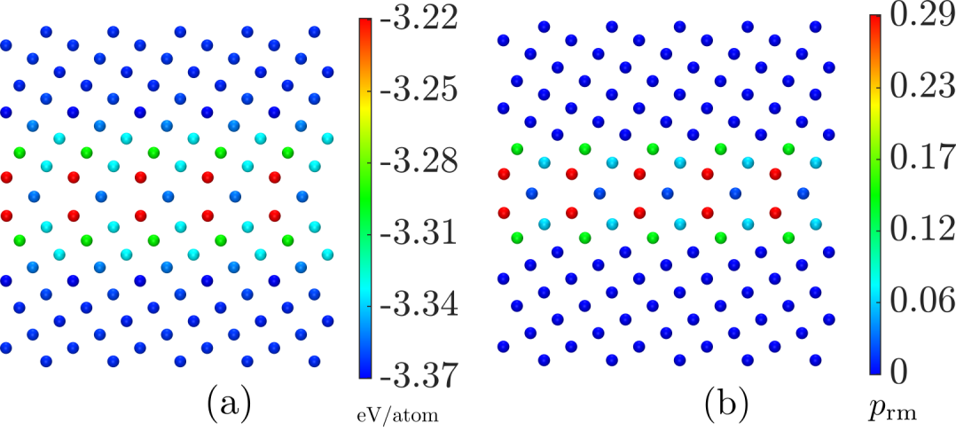
Figure 1: Illustration of removal probabilities. (a) The atomistic structure of $\Sigma 5(0\,\bar{2}\,1)$ GB, where the atoms are colored according to their energies. (b) The same $\Sigma 5(0\,\bar{2}\,1)$ GB structure is shown with the atoms colored according to their removal probabilities.

Similarly, the sites for atom insertion are also chosen stochastically within the GB. The importance of the insertion step has been highlighted in a Cu-Al binary alloy system [campbell2004copper], where the copper atoms preferentially segregate to the interstitial sites in the $\Sigma 5(3\,1\,0)$ Aluminum GB. This result underscores the importance of considering atom insertion steps during the Monte-Carlo simulation for achieving faster energy convergence.

The potential interstitial sites for inserting an atom in the GB region are determined through a Delaunay triangulation [lee1980two] of the GB atomistic structure. The circumcenters of the Delaunay tetrahedra provide the locations of the interstitial voids. For example, Figure 2(a) shows the voids that are identified at the circumcenters of the Delaunay tetrahedra of the $\Sigma 3(1\,0\,\bar{1})$ GB . To simplify presentation, we show only one Delaunay tetrahedron within the GB. A magnified version of this tetrahedron and the void is shown in Figure 2(b). The radius of the interstitial void is given by $r_{in}=r_{s}-r_{a}$, where $r_{s}$ is the radius of the circumsphere of the Delaunay tetrahedron and $r_{a}$ is the radius of the atom.

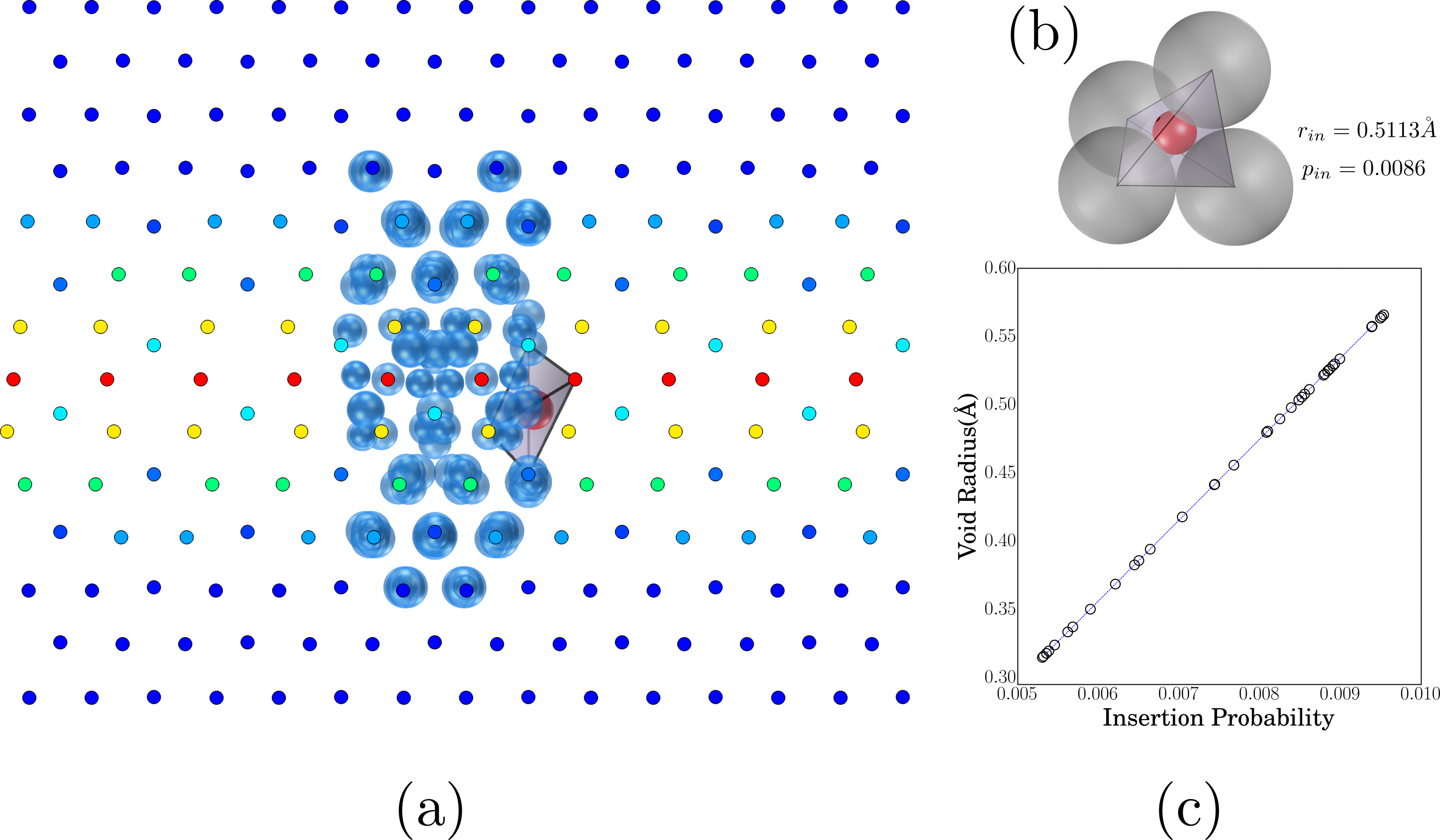
Figure 2: Illustration of insertion probabilities. (a) The atomistic structure of an asymmetric tilt GB, $\Sigma 3(1\,0\,\bar{1})$, is shown along with the voids present in the GB structure. The voids are obtained by meshing the GB structure and computing the circumcenters of the Delaunay tetrahedra. One such tetrahedron is shown in the GB structure and its magnified version is illustrated in (b). The radius of the void is given by the difference between the radius of the circumsphere and the atom radius. The probability of atom insertion is directly proportional to the void radius, as shown in (c).

In a recent study, we showed that the interstitial voids, determined using the circumcenters of the Delaunay tetrahedra, accurately predict the sites of hydrogen segregation in certain Ni GBs (refer to Figure S30 in [banadaki2017three]). Once the radii of all the interstitial voids within the GB region are computed, one of the sites is chosen stochastically with the probability:

$$p_{\text{in},i}=\frac{r_{v,i}}{\sum_{j=1}^{N_{v}}(r_{v,j})}$$ (2)

where $r_{v,i}$ is the radius of the $i^{th}$ void, $N_{v}$ is the total number of GB interstitial sites considered, and $\sum p_{\text{in},i}=1$. Figure 2(c) shows the insertion probabilities $p_{in}$ for the voids in $\Sigma 3(1\,0\,\bar{1})$ GB, and, as expected, $p_{in}$ is proportional to $r_{v,i}$. In summary, the trial moves consist of stochastically choosing either an atom to remove or an interstitial site for atom insertion. After the appropriate trial move, the new structure is relaxed at $0\text{\,}\mathrm{K}$ in LAMMPS [plimpton1995lammps]. If the difference in the GB energy before and after the trial move is denoted by $\Delta\gamma$, the new GB configuration is accepted if $\Delta\gamma<0$. If $\Delta\gamma>0$, the new GB configuration is accepted with a probability of $\exp\left(\frac{-\Delta\gamma\times A_{\text{GB}}}{k_{B}T_{R}}\right)$, where $A_{\text{GB}}$ is the area of the GB in the simulation box, $k_{B}$ is the Boltzmann constant and $T_{R}$ is the material specific reference temperature. Upon acceptance of a trial perturbation, the GB energy and configuration are updated and the perturbations are repeated for the new structure. Otherwise, the perturbed structure is discarded and the trial moves are repeated. As a summary, the MC algorithm is illustrated as a flowchart in Figure 3.

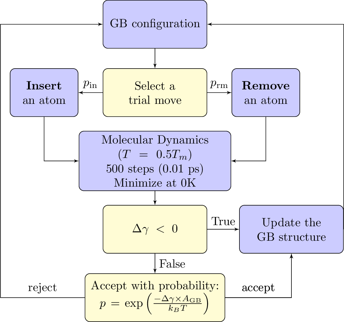
Figure 3: A flowchart of different steps involved in simulating a GB using the proposed Monte-Carlo simulation technique.

Results and Discussion

To test the efficiency of this Monte Carlo scheme, we simulated the set of 388 GBs in Aluminum and Nickel from Olmsted et al. [olmsted2009survey] and the set of 408 GBs in $\alpha$-Iron from Ratanaphan et al. [ratanaphan2015grain]. The interatomic potentials used to simulate these GBs are also identical with the exception of Aluminum where a more accurate Embedded Atom Method (EAM) potential developed by Mishin et al. [mishin1999interatomic] is utilized. This EAM potential function has been shown to reproduce the material parameters crucial for interface simulations - the cohesive energy, lattice parameter and the stable and metastable stacking fault energies - with reasonable accuracy when compared to density functional theory computations. For Al, to account for the change in EAM potential, we repeated the brute force energy calculations for the 388 GBs.

For the Monte Carlo simulations, the initial configuration for each GB is generated by choosing a random set of the microscopic DOF (i.e., the relative bicrystal displacement and boundary-plane translation along the normal vector). The bicrystallographic aspects, required for simulating the GBs in LAMMPS, are computed using the the GBpy software (https://pypi.python.org/pypi/GBpy) developed by the authors [banadaki2015efficient].

We find that, in most cases, the proposed Monte Carlo scheme finds the lowest-energy structure (as compared to the energies reported in [olmsted2009survey] and [ratanaphan2015grain]) for GBs in FCC (Al and Ni) and BCC ($\alpha$-Fe) metallic systems in just $\mathbf{5000}$ steps for the chosen reference temperature $T_{R}=0.5T_{m}$, where $T_{m}$ is the melting temperature, and a value of $p_{\text{rm}}=0.5$. The $5000$ steps include both accepted and rejected trial moves in the Monte Carlo scheme. We tried the values of $T_{R}=(0.25,0.5,0.75)T_{m}$ and $p_{\text{rm}}=0.25,0.5,0.75$ while optimizing the MC algorithm. The parameters finally chosen ($T_{R}=0.5T_{m}$ and $p_{\text{rm}}=0.5$) had the highest rate of energy convergence when compared to the brute-force algorithm.

In Figure 4, we compare the performance of the proposed algorithm by plotting a histogram of the error percentage defined as:

$$\text{\% Error}=\frac{\gamma^{\text{Monte-Carlo}}-\gamma^{\text{Brute-Force}}}{\gamma^{\text{Brute-Force}}}\times 100$$ (3)

That is, % Error the difference in the energies obtained from the MC and the brute-force techniques divided by the brute-force energy. The histogram reports the % Error for all the 1184 simulated interfaces (388 Al, 388 Ni and 408 $\alpha$-Fe GBs). This figure illustrates the accuracy with which the minimum energy GB structures are realized in the Monte Carlo scheme—approximately 96% of the 1184 GBs simulated have an error less than 1% and only about 0.6% of the GBs exhibited an error greater than 3%. The maximum error is $\sim 4.8\%$ for $\Sigma 315(2\,1\,3)(\bar{1}\,\bar{2}\,\bar{3})$ GB of $\alpha$-Fe. About 11% of the GBs show an error less than $-1\%$, which indicates that, in some cases, the Monte Carlo scheme results in lower energy structures than the ones obtained through the brute force simulations. Finally, in Figures S1, S2 and S3, the % error is illustrated in the complete 5-D phase space of the GBs (i.e. as a function of the five macroscopic crystallographic DOF of GBs). It is evident from these figures that there are no obvious correlations between GB crystallography and % Error.

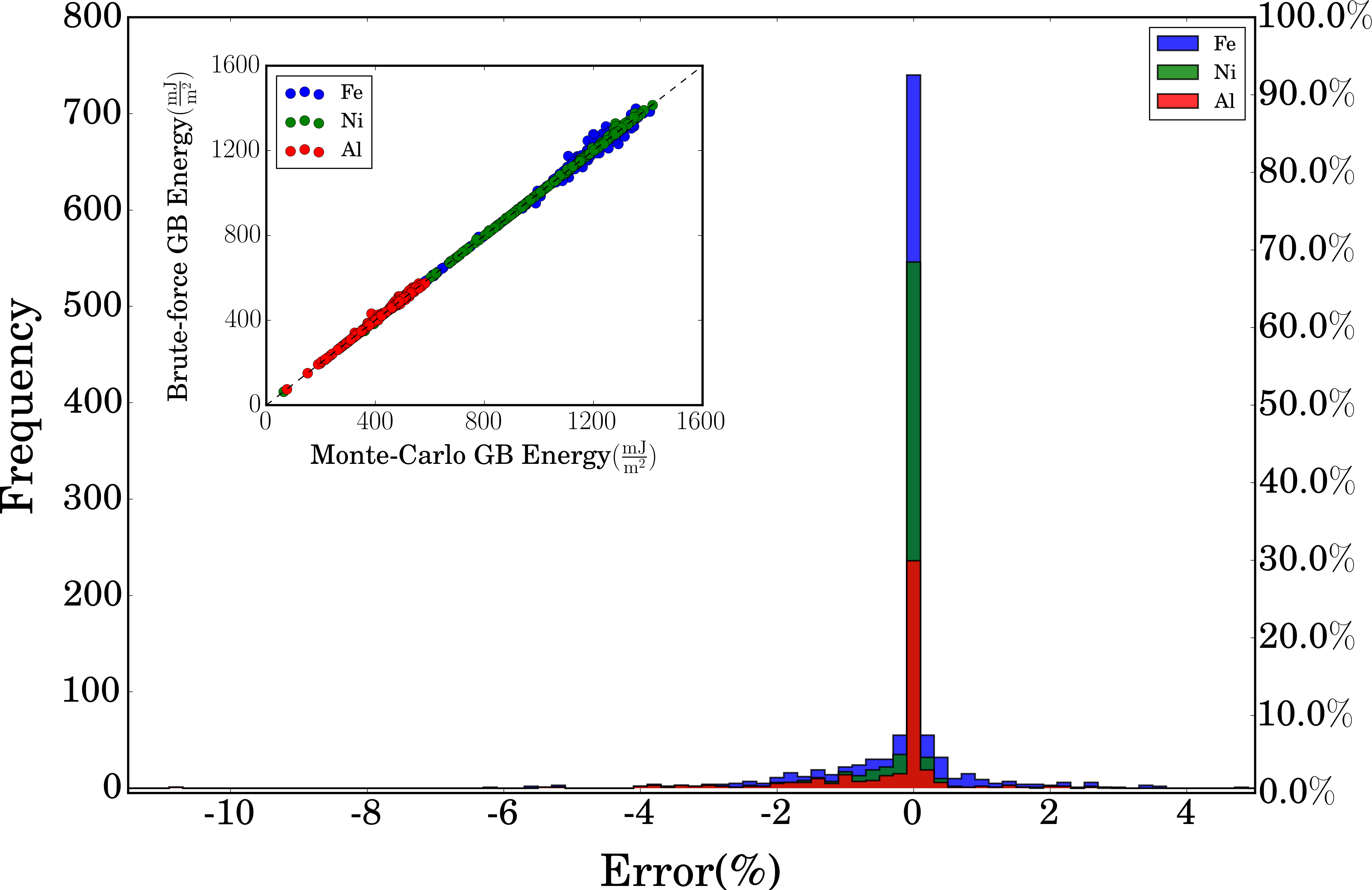
Figure 4: A stacked histogram of the Error (%) for the 388 GBs of Aluminum, 388 GBs of Nickel and 408 GBs of $\alpha$-Iron is shown. A negative value indicates that the energy obtained through the Monte Carlo scheme is lower than that obtained using the brute-force algorithm (i.e., the MC scheme provides a better estimate for the lowest-energy structure of the GB for these cases). Also shown in the inset is a correlation plot between the energies obtained through the MC vs. the brute-force algorithm.

We also tested the influence of the initial configuration on the performance of the MC simulations for Aluminum GBs (as we have access to a diverse set of GB structures from the brute-force simulations). In addition to the random configuration, we performed the MC simulations with two additional configurations as the initial state:

• Maximum-energy: GB structure corresponding to the highest-energy configuration from the brute-force simulations.

• Most-frequent: GB configuration that occurs with highest frequency in the brute-force simulations but does not correspond to the lowest-energy state. This structure may represent a deep local minimum in the energy landscape.

In Figure 5, we plotted the error percentages for MC simulations with random initial configurations. In Figures 6 and 7, the error percentages for the MC simulations with initial configuration as maximum-energy and most-frequent structures are plotted, respectively. The maximum-energy structure performs poorly compared to the random or the most-frequent structure. To compare the performance of these simulations with different initial structures, we will use the sum of the errors greater than zero. That is, we use the quantity $\sum_{i}\max\left(0,\gamma_{\tiny{\mbox{MC}}}-\gamma_{\tiny{\mbox{BF}}}\right)$, where $\gamma_{\tiny{\mbox{MC}}}$ and $\gamma_{\tiny{\mbox{BF}}}$ are the GB energies obtained using the Monte-Carlo and Brute-Force simulations, respectively. For the maximum-energy, the most-frequent, and the random initial structures, this quantity results in 109.5 mJ/m², 89.5 mJ/m² and 26.4 mJ/m², respectively. That is, the simulations where the initial structures correspond to the maximum-energy configurations perform the worst, but the most-frequent initial structure is not far behind. These results are not unexpected given that the simulations with the maximum-energy structure as the initial configuration can be interpreted as the worst-case scenario for the MC algorithm. For the most-frequent initial structure case, the larger errors may be due to the fact that the GB structure is getting stuck in a local minimum.

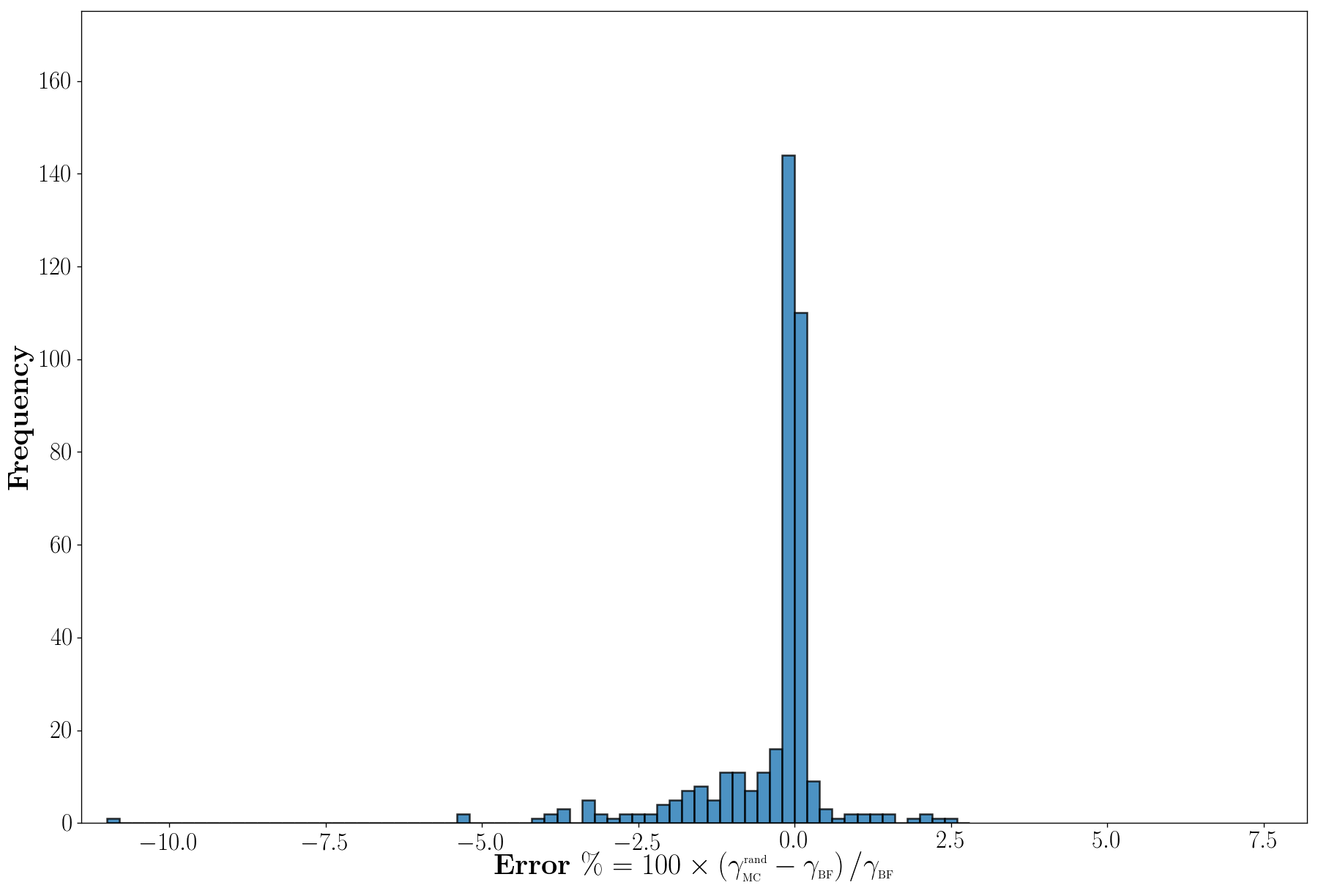
Figure 5: Histogram of the Error (%) for the 388 GBs of Aluminum is shown. The initial configurations for the MC simulations are constructed with random microscopic DOF.

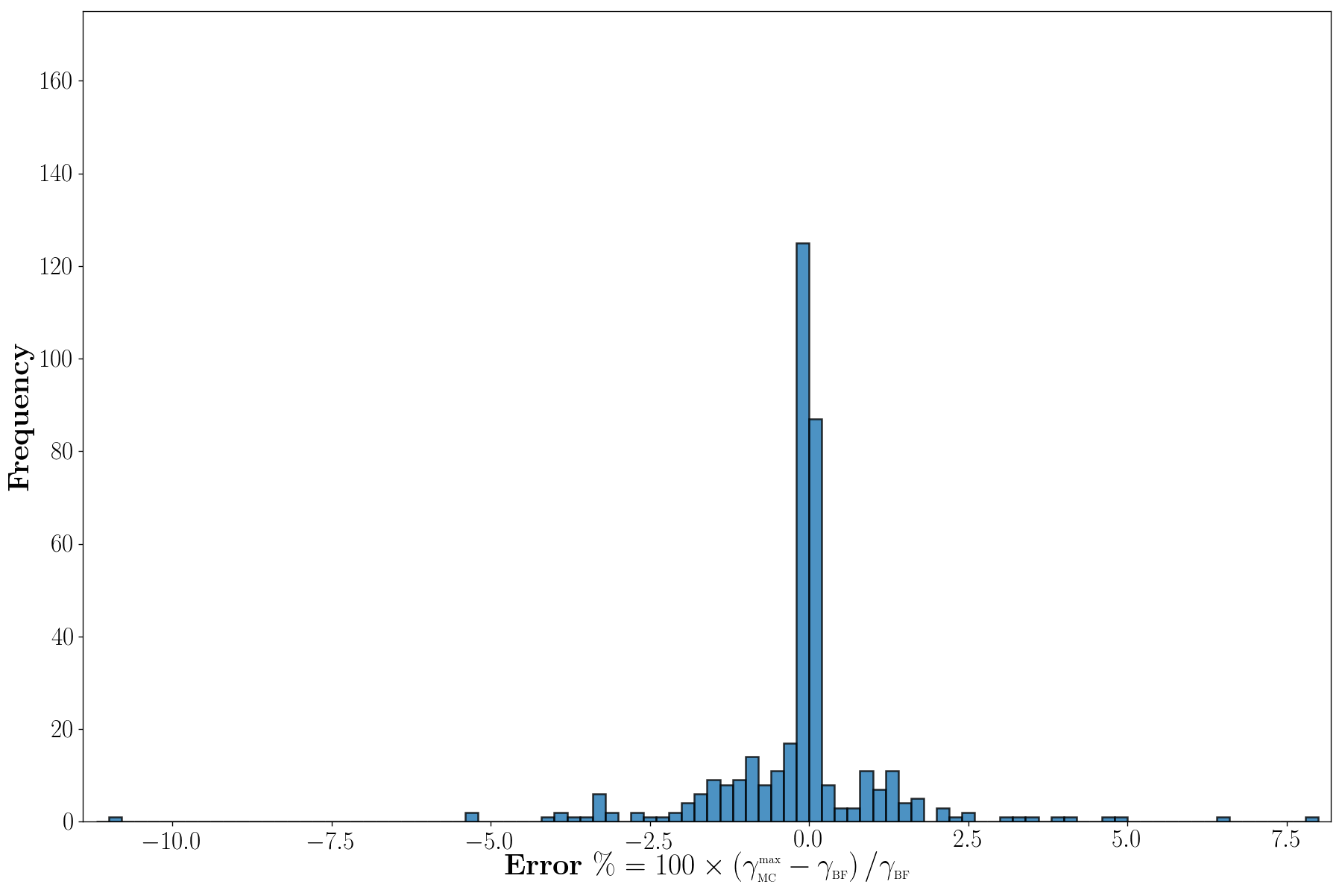
Figure 6: Histogram of the Error (%) for the 388 GBs of Aluminum is shown. The initial configurations are the maximum energy structures obtained from the brute-force simulations performed for Aluminum GBs.

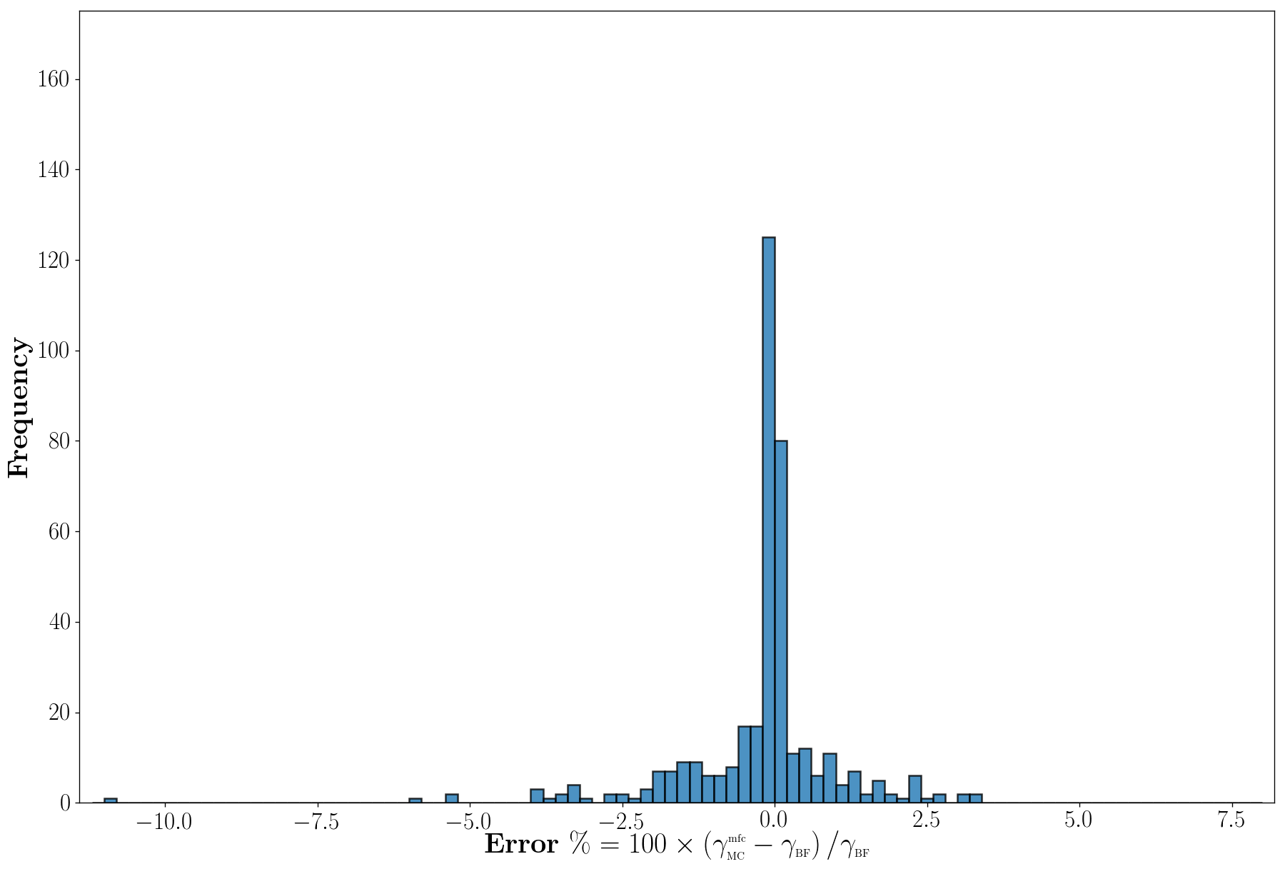
Figure 7: Histogram of the Error (%) for the 388 GBs of Aluminum is shown. The initial configurations correspond the most frequent structures (other than the minimum energy structure). These structures are obtained from the brute-force simulations performed for Aluminum GBs.

To better understand the influence of atom insertion and removal on GB structures, we provided a comparison of the range of excess-volumes sampled by the GB structures obtained through the Monte-Carlo and the brute-force simulations. For this analysis, we chose three Aluminum GBs: (a) $\Sigma 3\left(1\,0\,\bar{1}\right)$, (b) $\Sigma 17\left(1\,0\,0\right)$ and (c) $\Sigma 77\left(9\,\bar{5}\,2\right)$ and, in Figure 8, plotted the GB energies vs. the excess-volume per unit area (in units of lattice constant). In (i) and (ii), the excess-volumes of the Monte-Carlo and brute-force simulations are plotted, respectively. It is evident from the scatter in these plots, the diversity of the GB structures sampled is much more pronounced than those observed in the brute-force simulations. Therefore, it is reasonable to infer that a diverse set of GB structures are sampled by simply applying the atom removal and insertion perturbations. Furthermore, the effect of the trial perturbations on GB energies is evaluated by plotting the evolution of GB energies during the MC simulation for a few exemplary cases in section S2. The atom removal and insertion moves are, in some sense, drastic enough that they change both the GB energies and structures considerably. While we refer the reader to section S2 for a complete discussion on the trends in the energy evolution during the MC simulations, we would like to point out that the MC simulations not only provide the lowest-energy GB structure but also sample important metastable states [han2016grain].

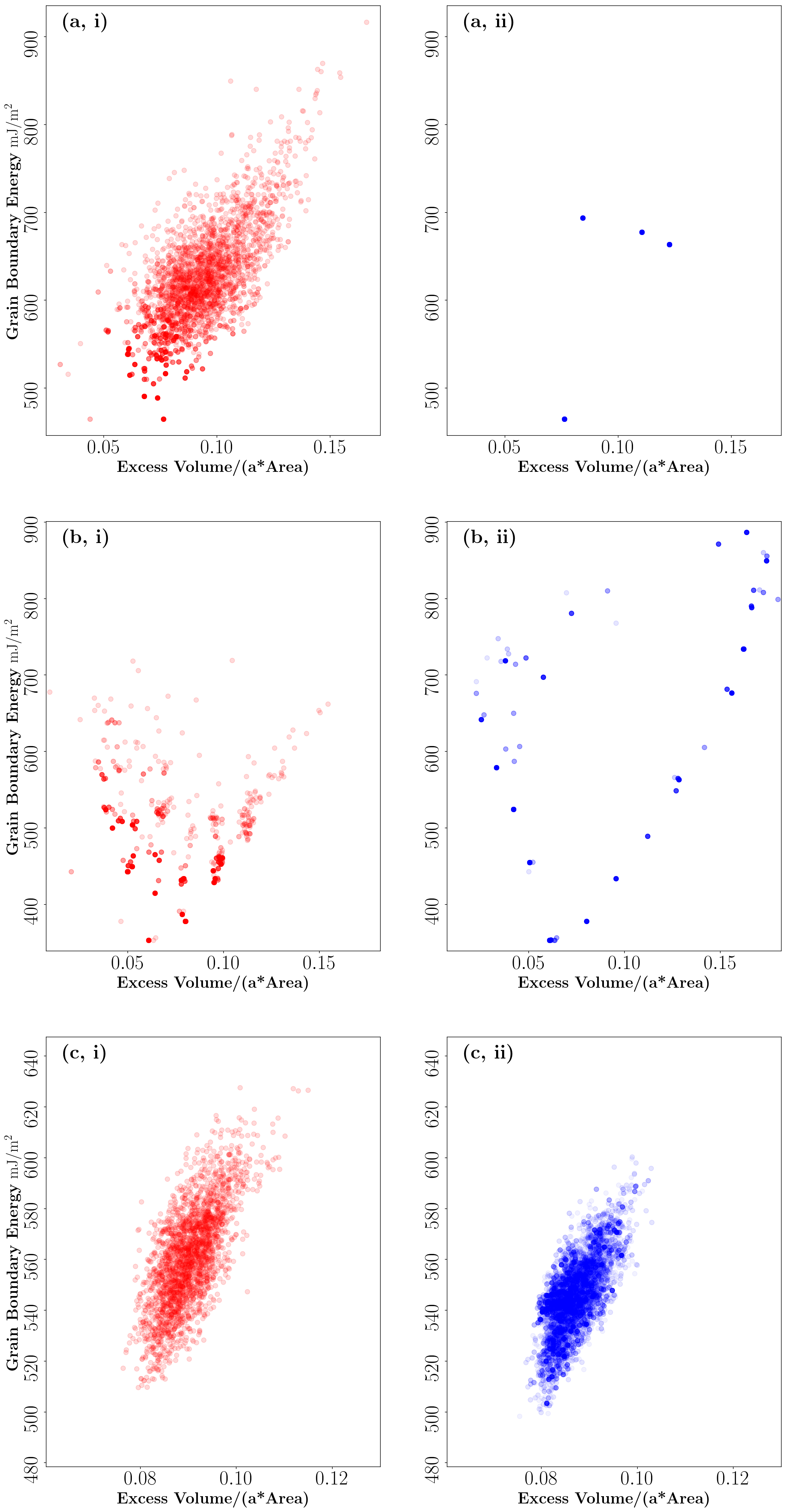
Figure 8: The energies are plotted against the normalized excess volume per unit area for three Aluminum GBs: (a) $\Sigma 3\left(1\,0\,\bar{1}\right)$, (b) $\Sigma 17\left(1\,0\,0\right)$ and (c) $\Sigma 77\left(9\,\bar{5}\,2\right)$. In (i), the excess volume of the GB structures from the Monte-Carlo simulation are plotted. The structures are the relaxed structures of the accepted trail perturbations. As a comparison, the excess-volume of the relaxed GB structures obtained from the brute-force simulations are plotted in (ii).

We use the example of the evolution of structures and energies of $\Sigma 5\left(0\bar{1}3\right)$ GB, in Nickel, to illustrate how the MC simulations could shed light on GB metastability. The structural aspects of $\Sigma 5\left(0\bar{1}3\right)$ GB have been analyzed as function of temperature [frolov2013effect, frolov2013structural, frolov2014effect, freitas2018free] and, more recently, it has been shown that, in Copper, this GB exhibits a phase-transition at approximately 184 $\pm$ 4 Kelvin [freitas2018free] from a structure that contains “normal-kites” to a structure that contains “split-kites” [frolov2013effect]. To compute the phase-transition temperature using the technique developed in [freitas2018free], both the 0K lowest-energy and the relevant metastable structures have to be determined a priori. In the MC simulations, GBs that are sampled frequently but do not correspond to the lowest-energy structure can be considered as relevant metastable structures. For example, consider the plot of the energies vs. MC step number for the $\Sigma 5\left(0\bar{1}3\right)$ Nickel GB shown in Figure 9. In this plot, we highlight three GB structures, labeled (a), (b) and (c), that correspond to the top three most sampled structures during the MC simulation.

The lowest-energy GB structure with normal-kite units is shown in Figure 10(a) and has been observed about 307 times (out of 5000) during the Monte-Carlo simulation. However, there are two other structures with higher energies that are observed more frequently than the lowest-energy structure. These GBs are labeled (b) and (c) in Figure 9 and are shown in Figure 10 (b) and (c), respectively. The structure in Figure 10(b) is obtained by simply introducing an interstitial in one of the normal-kite units and has been observed about 326 times. The structure in Figure 10(c) exhibits the split-kite structure, has the highest frequency, and has been observed about 388 times during the Monte-Carlo simulation. The split-kite structure may very well have been the equilibrium structure, for the $\Sigma 5\left(0\bar{1}3\right)$ GB, at the temperature used in the Boltzmann acceptance probability (T = 0.5T_m). Therefore, it is important to note that the MC algorithm introduced in this article not only generates the lowest-energy structures but also provides the most relevant metastable structures. Once these metastable structures are determined, techniques such as thermodynamic integration [frolov2015segregation, freitas2018free] could be used to determine the phase transitions of GBs.

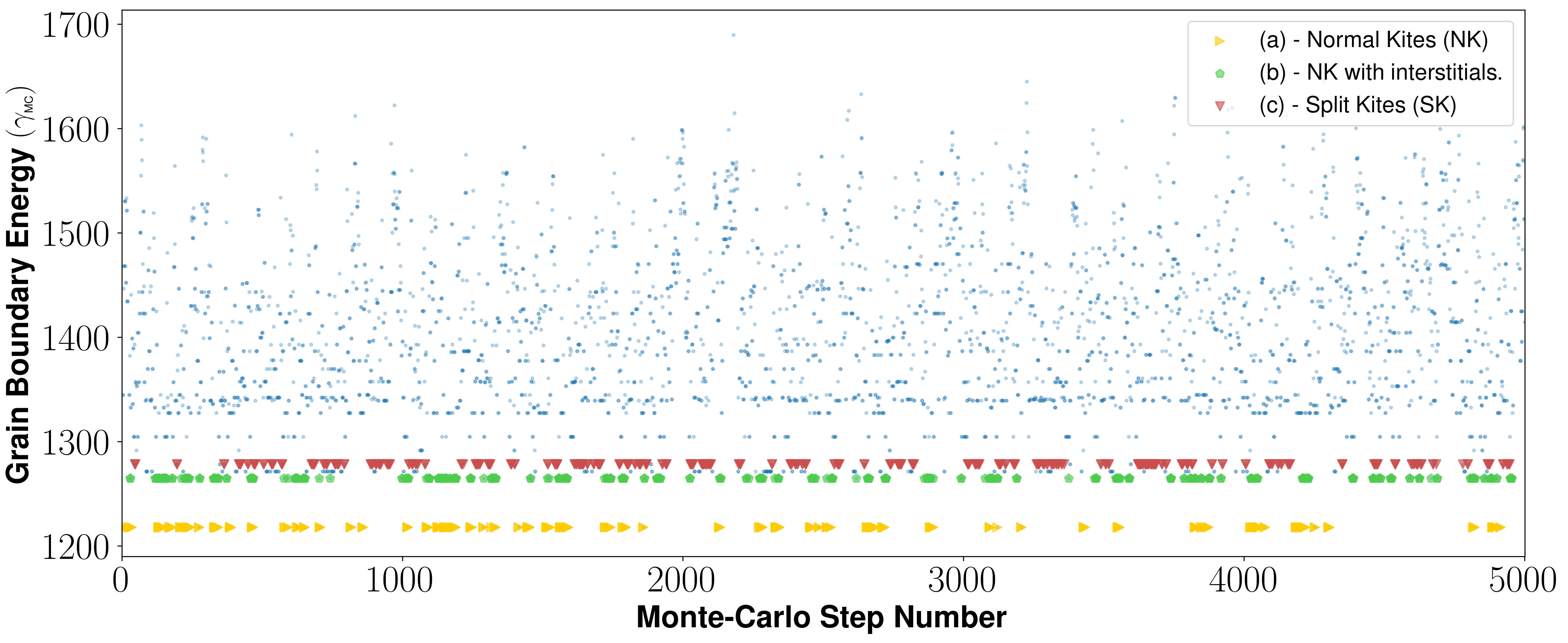
Figure 9: A scatter plot of GB energies vs. the Monte-Carlo step number is shown. Highlighted are the three most frequently observed GB structures during the Monte Carlo simulation. (a), (b) and (c) were observed 307, 326 and 388 times, respectively during the simulation. The structures of these GBs are shown in Figure 10.

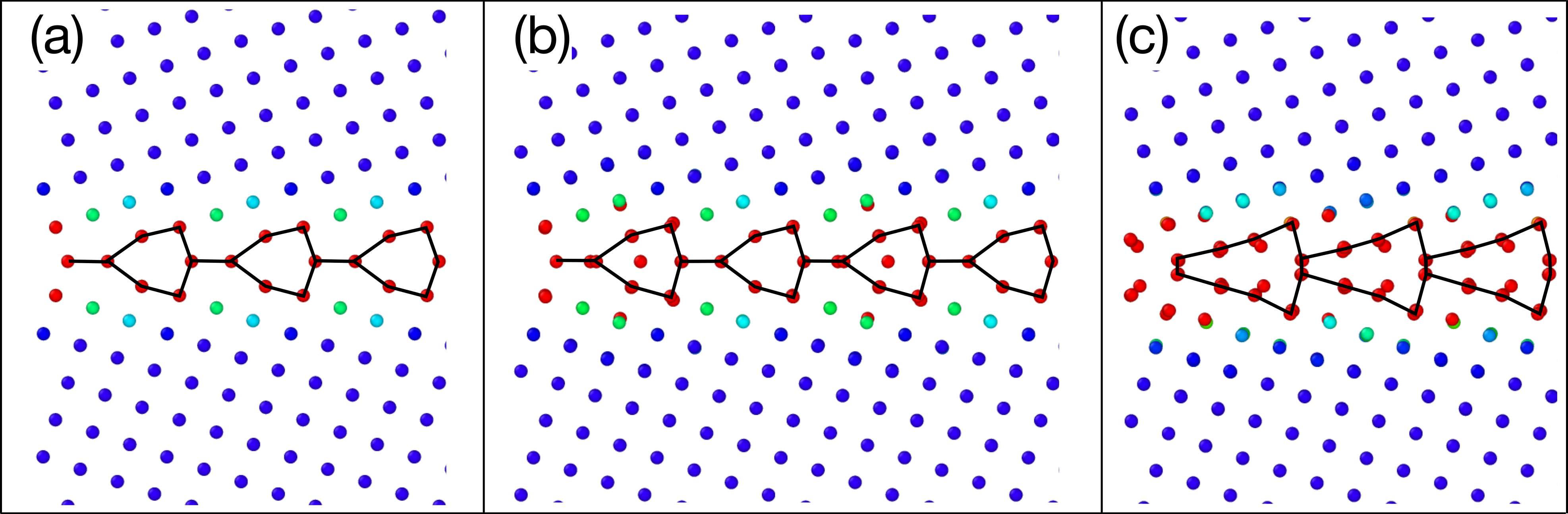
Figure 10: Three structures of $\Sigma 5\left(0\bar{1}3\right)$ GBs are illustrated in the decreasing order of frequency with which they are observed during the Monte-Carlo simulation. (a) The structure with the lowest energy exhibits normal-kites and is observed approximately 307 times of the 5000 Monte-Carlo steps. (b) This structure is observed approximately 326 times, has one normal-kite unit and another with an interstitial. (c) This GB structure has the split-kite units and has been observed approximately 388 times.

Finally, as mentioned in the introductory paragraphs of the article, the MC algorithm is computationally more efficient than the brute-force technique in generating low-energy GB structures. To give an indication of the improved computational efficiency, Table 1 provides the amount of time required to generate low-energy structures for 15 GBs, ordered according to computational expense, with differing bicrystallography. Since the number of simulation steps required in the brute-force algorithm depends on the bicrystallographic symmetry, the relative performance also depends on the GB type. In this table, explicit comparisons for the time required to generate the minimum energy structures for 15 GBs, with computation times varying from minimum to maximum, are shown.

Table 1: The efficiency of the Monte-Carlo simulation, as compared to the brute-force algorithm, is illustrated by tabulating the time (in mins) taken by each algorithm to generate the low energy GB structure. Both the brute-force and the Monte-Carlo simulations for each GB were performed on a single compute node with 16 cores, and 64 GB memory.

GB Crystallography	Brute-Force (mins)	Monte-Carlo (mins)	Relative Performance
$\Sigma 3(1\,1\,1)(\bar{1}\,\bar{1}\,\bar{1})$	813	166	4.89
$\Sigma 27(1\,\bar{1}\,5)(1\,\bar{1}\,\bar{5})$	1875	119	15.76
$\Sigma 101(1\,0\,0)(\bar{1}\,0\,0)$	5563	319	17.44
$\Sigma 29(0\,\bar{2}\,5)(0\,\bar{2}\,\bar{5})$	1438	154	9.33
$\Sigma 105(3\,1\,5)(\bar{1}\,\bar{3}\,\bar{5})$	2188	140	15.63
$\Sigma 63(\bar{1}\,10\,\bar{5})(\bar{1}\,\bar{5}\,10)$	1875	200	9.37
$\Sigma 111(11\,\bar{10}\,\bar{1})(\bar{10}\,11\,\bar{1})$	2750	1526	1.80
$\Sigma 57(3\,\bar{5}\,2)(\bar{2}\,5\,\bar{3})$	4438	158	28.09
$\Sigma 93(5\,\bar{6}\,1)(\bar{1}\,6\,\bar{5})$	4625	197	23.48
$\Sigma 111(1\,1\,1)(\bar{1}\,\bar{1}\,\bar{1})$	4719	165	28.60
$\Sigma 55(\bar{3}\,\bar{1}\,0)(3\,1\,0)$	9563	158	60.52
$\Sigma 99(\bar{4}\,1\,1)(4\,\bar{1}\,1)$	9844	166	59.30
$\Sigma 95(0\,\bar{1}\,3)(1\,0\,\bar{3})$	5125	193	26.55
$\Sigma 77(\bar{9}\,5\,2)(9\,\bar{5}\,2)$	4438	287	15.46
$\Sigma 109(1\,0\,0)(\bar{1}\,0\,0)$	5156	325	15.87

On average the Monte Carlo simulations (for 5000 trial moves) were about 20 times more efficient. One reason for the efficiency is the fewer number of minimization steps required in the MC scheme. The other is related to the local nature of the MC perturbations. The computational time, to minimize a structure in the MC scheme, is a lot less than that required to minimize the bicrystal configurations created in brute force algorithms.

It is important to note that the 5000 steps correspond to the total energy minimizations, including accepted and rejected moves, performed for each GB. Therefore, 5000 is not an ensemble average of many GBs but it is the maximum number of steps required to get within 5% of the brute-force energy for all 1184 GBs. In the plot below (Figure 11), we show a histogram of the step number (corresponding to the first Monte Carlo step when the minimum GB energy was obtained) for all the 388 Aluminum grain boundaries. The initial structure for the GBs is the maximum energy structure from the brute-force simulations. It is clear from this plot that for most of the GBs, the minimum energy structure is recovered within the first 2000-3000 steps.

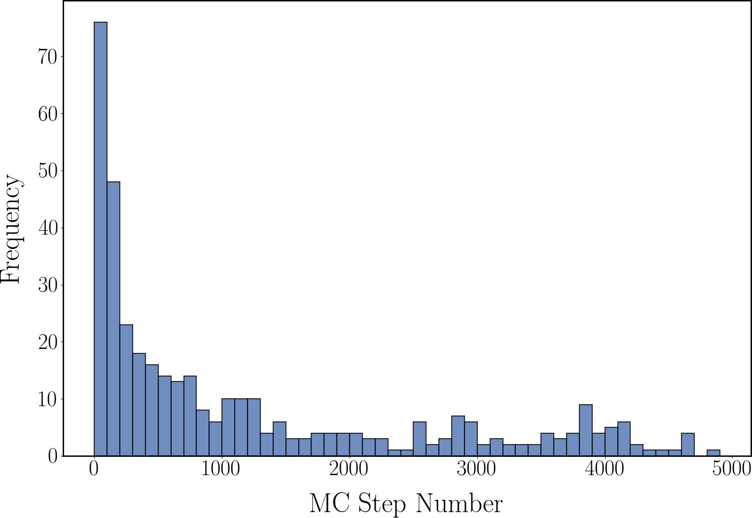
Figure 11: The frequency of the Monte Carlo step numbers when the minimum energy structure is encountered for the 388 GBs in Aluminum. The initial structure is the maximum energy GB from the brute-force simulations.

Conclusions

In conclusion, we present a novel and efficient technique for generating the low-energy $0\text{\,}\mathrm{K}$ structures for both FCC and BCC metallic GBs. It is observed that the Monte Carlo algorithm developed in this article is on average an order of magnitude faster than the traditional brute-force technique. Since the number of simulations in a brute-force algorithm depends on the symmetry aspects of the interface, the efficiency achieved by the MC simulation is shown for fifteen exemplary cases in Table 1. While it is well recognized that it is necessary to change the number of atoms in an interface to access the different energetic states, prior techniques have relied primarily on removal [von2006structures], swapping of atoms [sadigh2012scalable, pan2016effect], or on the insertion of atoms randomly in the GB structure [zhu2018predicting, frolov2018grain]. The novel aspect of our algorithm is the geometrically-informed atom insertion as a perturbation step, which results in an efficient convergence to lower energy states of the GB.

More recently, the importance of analyzing metastable GB states has been highlighted by Han et al. [han2016grain]. The proposed MC algorithm will also help sample these meta-stable states as the trial perturbations visit a large and diverse range of GB structures. Therefore, this algorithm not only allows for an efficient simulation of low-energy GB structures, but also provides a means to compute thermodynamic equilibrium properties. To this end, we are currently extending the MC framework to a hybrid Monte-Carlo/Molecular-Dynamics scheme [sadigh2012scalable]. Compared to the genetic algorithms that perform grand-canonical based optimization of GB structures [chua2010genetic, zhu2018predicting, frolov2018grain], the Monte-Carlo technique has the advantage that the acceptance probabilities can be tailored to satisfy detailed balance equations for different ensembles. For example, in [hudson2006grand], detailed balance equations, for performing grand canonical Monte Carlo simulations, have been developed for inter-granular glassy films. Similar equations can be extended to the GBs and thermodynamic equilibrium properties, such as the free energy as a function of temperature, can be computed in a variety of relevant statistical ensembles.

This MC simulation scheme is general enough and can be easily extended to multi-component systems. We anticipate that adding the atom-insertion step to the traditional hybrid Monte-Carlo/Molecular-Dynamics algorithm [sadigh2012scalable], which only contains the atom swapping events, will result in a faster convergence, particularly when the size difference between the solute and solvent atoms is large.

Data availability

The raw/processed data required to reproduce these findings cannot be shared at this time as the data also forms part of an ongoing study.

References

Supplemental Materials:
An Efficient Monte-Carlo Algorithm for Extracting the Minimum Energy Structure of Metals

S1 Error in the Five-Parameter GB Space

In Figures S1, S2 and S3, the % Error is plotted for all the GBs simulated for Aluminum, Nickel and $\alpha-$Iron, respectively. The complete crystallography of the GB is provided by specifying the GB in the boundary-plane fundamental zone for each misorientation. Please refer to [patala2013symmetries] for further details on GB representation.

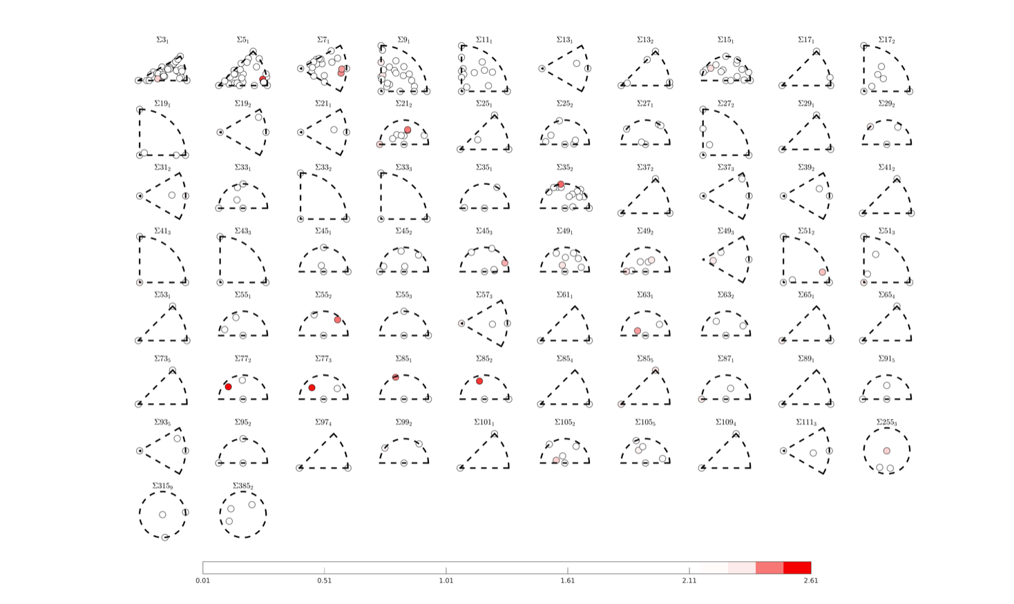
Figure S1: An illustration of the level of error for Aluminum simulations based on the location of the stereographic projection of the boundary plane of the GB on the fundamental zones of each $\Sigma$ rotation that has been included in the data-set.

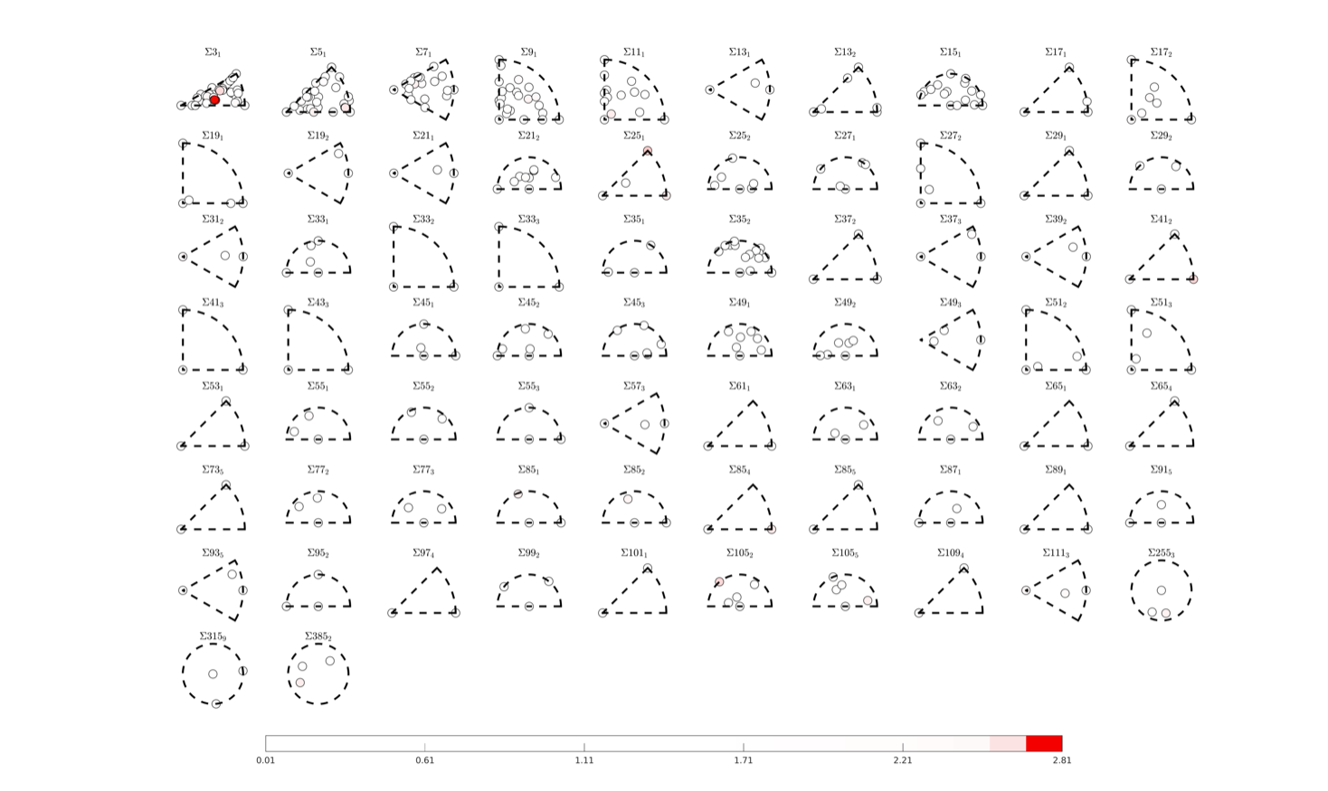
Figure S2: An illustration of the level of error for Nickel simulations based on the location of the stereographic projection of the boundary plane of the GB on the fundamental zones of each $\Sigma$ rotation that has been included in the data-set.

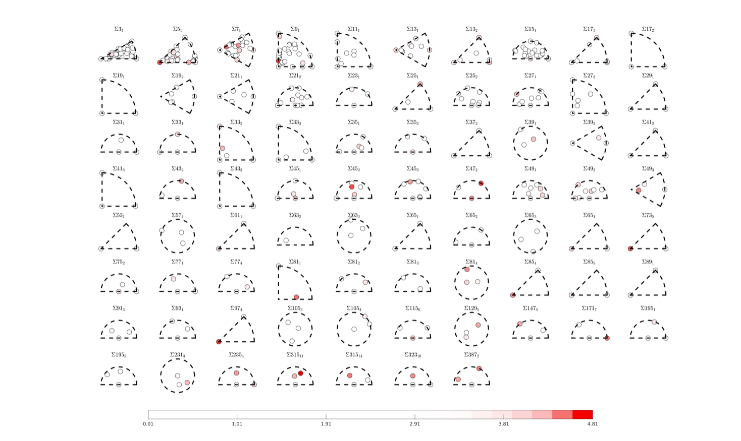
Figure S3: An illustration of the level of error for $\alpha$-Iron simulations based on the location of the stereographic projection of the boundary plane of the GB on the fundamental zones of each $\Sigma$ rotation that has been included in the data-set.

S2 Evolution of GB Energy in the Monte Carlo Scheme

The Monte Carlo perturbations (corresponding to either the removal or the insertion of atoms) change the structure enough that, we believe, the GB jumps from one local minima to another. For example, shown in figures S4 to S6 are three different cases that reflect the evolution of energy as a function of Monte-Carlo steps. These simulations correspond to the Aluminum GBs with the maximum-energy structure as the initial configuration. In general, the energy fluctuates a lot with each perturbation corresponding to atom removal or insertion. Qualitatively, we classified the trends in energy fluctuations, for the 388 GBs of Aluminum, into the following categories:

1. GBs where the lowest energy state is visited reasonably frequently. These GBs visited the lowest energy structure about 5 to 500 times during the MC simulation. This seems to be the most likely case for the evolution of GB energies, i.e. there are about 267 GBs ($\sim 69\%$) that show this behavior. Three examples are shown in figure S4.

2. The cases where the lowest energy state is visited very frequently. These GBs visited the lowest energy structure more than 500 times during the MC simulation. There are about 26 GBs ($\sim 7\%$) that show this behavior. Three examples of such evolution are shown in figure S5.

3. GBs where the lowest energy state is visited very infrequently. These GBs visited the lowest energy structure less than 5 times during the MC simulation. There are about 95 GBs ($\sim 24\%$) that show this behavior. Three examples of such behavior are shown in figure S6.

We also show a few cases where a large increase in the energy is observed during the MC simulation (figure S7). This is not unexpected in MC simulations because of a finite (albeit very low) probability of acceptance of perturbations that lead to a large increase in energy.

Finally, in figures S8, S9, S10, and S11, we plotted the energy evolution during MC simulations with distinct initial configurations (maximum-energy, most-frequent and random), for $\Sigma 21(7\,5\,\bar{4})$, $\Sigma 21(\bar{1}\,0\,\bar{3})$, $\Sigma 35(8\,\bar{5}\,\bar{11})$, and $\Sigma 5(5\,\bar{11}\,8)$ GBs, respectively. As such there is no discernible difference in the evolution of energies after a few initial MC trial moves. The specific GBs are chosen to show a diversity in the minimum energy configurations obtained.

• The maximum-energy initial configuration resulted in the lowest energy structure for $\Sigma 21(7\,5\,\bar{4})$ GB (Figure S8)

• For $\Sigma 21(\bar{1}\,0\,\bar{3})$ GB, (Figure S9), the random configuration gave the lowest energy structure.

• For $\Sigma 35(8\,\bar{5}\,\bar{11})$ and $\Sigma 5(5\,\bar{11}\,8)$ GBs (Figures S10 and S11), starting with the most-frequent configuration gave the lowest energy structure.

(a) $\Sigma 41(0\,\bar{1}\,9)(0\,\bar{1}\,\bar{9})$

(b) $\Sigma 25(5\,\bar{4}\,\bar{3})(\bar{4}\,5\,\bar{3})$

(c) $\Sigma 9(1\,\bar{1}\,1)(\bar{1}\,1\,\bar{5})$

Figure S4: The low energy state is visited with reasonable frequency. This seems to be the most likely case.

(a) $\Sigma 3\left(1\,1\,1\right)\left(\bar{1}\,\bar{1}\,\bar{1}\right)$

(b) $\Sigma 5\left(10\,\bar{1}\,3\right)\left(\bar{10}\,\bar{1}\,\bar{3}\right)$

(c) $\Sigma 21\left(1\,1\,1\right)\left(\bar{1}\,\bar{1}\,\bar{1}\right)$

Figure S5: The lowest energy structure is visited very frequently.

(a) $\Sigma 15(\bar{2}\,\bar{1}\,0)(2\,1\,0)$

(b) $\Sigma 17(0\,\bar{1}\,4)(0\,\bar{1}\,\bar{4})$

(c) $\Sigma 9(8\,1\,5)(\bar{5}\,\bar{4}\,\bar{7})$

Figure S6: The lowest energy structure is rarely visited.

(a) $\Sigma 21(5\,\bar{4}\,\bar{1})(\bar{4}\,5\,\bar{1})$

(b) $\Sigma 17(1\,5\,5)(\bar{1}\,\bar{7}\,\bar{1})$

(c) $\Sigma 3(3\,1\,0)(\bar{8}\,1\,\bar{5})$

Figure S7: A few cases where the local perturbation results in a large increase in energy. Such a behavior is not unexpected in Monte Carlo simulations.

(a) Maximum Energy Structure; minimum energy found = 530.7 mJ/m²

(b) Most Frequent Structure; minimum energy found = 539.1 mJ/m²

(c) Random Structure; minimum energy found = 542.4 mJ/m²

Figure S8: The evolution of energies during the MC simulation for three initial configurations (a) the maximum energy structure, (b) the most frequent structure and (c) the random structure, for $\Sigma 21(7\,5\,\bar{4})(\bar{3}\,0\,1)$. The minimum energies found in each simulation are provided in the captions.

(a) Maximum Energy Structure; minimum energy found = 514.3 mJ/m²

(b) Most Frequent Structure; minimum energy found = 507.1 mJ/m²

(c) Random Structure; minimum energy found = 500.1 mJ/m²

Figure S9: The evolution of energies during the MC simulation for three initial configurations (a) the maximum energy structure, (b) the most frequent structure and (c) the random structure, for $\Sigma 21(\bar{1}\,0\,\bar{3})(1\,5\,8)$. The minimum energies found in each simulation are provided in the captions.

(a) Maximum Energy Structure; minimum energy found = 524.0 mJ/m²

(b) Most Frequent Structure; minimum energy found = 513.3 mJ/m²

(c) Random Structure; minimum energy found = 519.0 mJ/m²

Figure S10: The evolution of energies during the MC simulation for three initial configurations (a) the maximum energy structure, (b) the most frequent structure and (c) the random structure, for $\Sigma 35(8\,\bar{5}\,\bar{11})(\bar{8}\,11\,5)$. The minimum energies found in each simulation are provided in the captions.

(a) Maximum Energy Structure; minimum energy found = 490.6 mJ/m²

(b) Most Frequent Structure; minimum energy found = 488.4 mJ/m²

(c) Random Structure; minimum energy found = 493.3 mJ/m²

Figure S11: The evolution of energies during the MC simulation for three initial configurations (a) the maximum energy structure, (b) the most frequent structure and (c) the random structure, for $\Sigma 5(5\,\bar{11}\,8)(\bar{5}\,4\,\bar{13})$. The minimum energies found in each simulation are provided in the captions.

Supplemental References