The Betelgeuse Project II: Asteroseismology

Abstract

We explore the question of whether the interior state of massive red supergiant supernova progenitors can be effectively probed with asteroseismology. We have computed a suite of ten models with ZAMS masses from 15 to 25 M_⊙ in intervals of 1 M_⊙  including the effects of rotation, with the stellar evolutionary code MESA. We estimate characteristic frequencies and convective luminosities of convective zones at two illustrative stages, core helium burning and off-center convective carbon burning. We also estimate the power that might be delivered to the surface to modulate the luminous output considering various efficiencies and dissipation mechanisms. The inner convective regions should generate waves with characteristic periods of $\sim$ 20 days in core helium burning, $\sim$10 days in helium shell burning, and 0.1 to 1 day in shell carbon burning. Acoustic waves may avoid both shock and diffusive dissipation relatively early in core helium burning throughout most of the structure. In shell carbon burning, years before explosion, the signal generated in the helium shell might in some circumstances be weak enough to avoid shock dissipation, but is subject to strong thermal dissipation in the hydrogen envelope. Signals from a convective carbon-burning shell are very likely to be even more severely damped by within the envelope. In the most optimistic case, early in core helium burning, waves arriving close to the surface could represent luminosity fluctuations of a few millimagnitudes, but the conditions in the very outer reaches of the envelope suggest severe thermal damping there.

1 Introduction

Betelguese ($\alpha$ Orionis) is a massive red supergiant (RSG) that is destined to explode as a Type IIP supernova (some speculate explosion as a blue supergiant) and leave behind a neutron star. It is thus a touchstone for a broad range of issues of the evolution and explosion of massive stars. One of the outstanding issues is that we do not have tight constraints on the evolutionary state of Betelgeuse and hence when it might explode. Closely related issues are uncertainties about the internal rotational state and associated mixing. Understanding Betelgeuse in greater depth will yield benefits to the entire subject of massive star evolution.

As commanding as its presence is in the evening sky, its brightness limits certain aspects of the study of Betelgeuse. The distance is currently known to only 20% ($D=197\pm 45$ pc; Harper et al. 2008, 2017), and it is too bright to be observed by Gaia. This leaves key properties such as radius and luminosity somewhat uncertain. On the other hand, its closeness allows other key measurements since its image can be resolved (Haubois et al. 2009). A particularly interesting potential constraint on Betelgeuse is the rotational velocity ($\sim 15$ km s^-1) measured with $HST$ Dupree et al. (1987). Betelgeuse shows a 420 day period Dupree et al. (1987) that is most likely a first overtone radial pulsation mode that has not been broadly exploited as a constraint on Betelgeuse. It also shows variance on timescales of 2000 days that is associated with overturn of convective plumes. Many apparently single massive stars have undergone mergers. Could that be true of Betelgeuse?

For a judicious choice of distance, Betelgeuse might be brought into agreement with observations of $L$, $R$, and $T_{eff}$ at either the minimum–luminosity base of the red supergiant branch (RSB) or at the tip of the RSB. Single–star models give a rotational velocity of about that observed only near the minimum luminosity with the velocity at the tip of the giant branch being far below the suggested observed value. The former seems very improbable, and this phase disagrees with estimates of log $g$ and with the possible observed rate of contraction of the radius of Betelgeuse. The latter comports with standard assumptions, but cannot easily account for the claimed rotational velocity. In the first paper of The Betelgeuse Project (Wheeler et al., 2017), we showed that single-star models have difficulty accounting for the rapid equatorial rotation and suggested that Betelgeuse might have merged with a companion of about 1 M_⊙ to provide the requisite angular momentum to the envelope. Recent observations of Betelgeuse with ALMA are consistent with a rapid equatorial velocity (Kervella et al., 2018). This reinforces the notion that the results of Dupree et al. (1987) are due to systematic rotational motion rather than the motion of convective plumes and hence the need to understand this remarkably high equatorial velocity. Nevertheless, the convective plumes are real, as revealed also in the RSG Antares (Montargès et al., 2017), and Betelgeuse shows a variety of complex motion on its surface that calls for deeper understanding before the rotational velocity can be solidly confirmed.

We need another means to determine the inner evolutionary state of Betelgeuse and, by extension, any massive RSG. Specifically, to resolve the uncertainties of the mass and evolutionary state of Betelgeuse, we need to peer inside. The most logical tool is asteroseismology (Aerts, 2015). Stellar structure and evolution still is mostly pursued with spherical models not far removed from pioneering work by Hoyle, Schwarzschild and others. We should be prepared to find that the innards of real 3D RSG are interestingly different, as we have found for the Sun.

This work is an extension of Wheeler et al. (2017) and hence presented in the context of models for Betelgeuse, but the principles should apply to RSG more broadly. Section 2 presents our model evolutionary computations, §3 gives our results for characteristic frequencies generated near the base and the tip of the RSB, §4 addresses the possibility of detecting evidence of these waves at the surface, and §5 presents a discussion of our results.

2 Computations

We evolved a grid of models from the Zero Age Main Sequence (ZAMS) to near the onset of core collapse using the stellar evolution code Modules for Experiments in Stellar Astrophysics (MESA; Paxton et al. 2011, 2013). We computed models of solar metallicity with ZAMS masses from 15 to 25 M_⊙ at intervals of 1 M_⊙ primarily using MESA version 6208. Most of the rotating models employed version 7624. One suite of models were non–rotating and another suite with the same ZAMS masses began with an initial rotation of $\sim$ 200 km s^-1, corresponding to about 25% of the Keplerian velocity on the ZAMS. Because our principal goal was to explore the promise of an asterosesimological probe, we chose only the default prescriptions in MESA, Schwarzschild convection and an overshoot parameter of $\alpha=0.2$. For the rotating models, we again chose MESA default values of mechanisms of angular momentum transport and mixing. We did not include magnetic effects (Wheeler et al., 2015). We employed the “Dutch" mass–loss prescriptions with $\eta=0.8$. We used nuclear reaction network approx21. The inlist we employed is available upon request from the authors. For each ZAMS mass, the models were computed to the onset of core collapse. We present here data during early core helium burning at the base of the RSB and at the first episode of off-center carbon shell burning. The formal criterion we adopted in the latter case was that the central mass fraction of carbon be less than $10^{-5}$. By that criterion, a couple of the models were in a phase without convective carbon burning. We then chose models at slightly different times such that they did have off-center convective carbon burning for the sake of homogeneity of sampling the associated convective frequencies. Given the richness of the interior structure of massive stars and its sensitive variation with time, these choices are purely illustrative. Figure 1 illustrates the structure of the helium-burning stage for the non-rotating and rotating models of 20 M_⊙ and Figure 2 the non-rotating and rotating models in off-center carbon shell burning. Rotation as we have invoked it has relatively little effect on the inner structure. In the later stages there is relatively little difference in the outer, observable, characteristics as the models evolve (Wheeler et al., 2017). There are significant differences in the inner convective motions that change rapidly with time that might give asteroseismological clues to the evolutionary state. In the following discussion, we refer to specific models by their ZAMS mass.

Figure 1 and panel (b) of Figure 2 are characteristic of many of the models by showing a convective region around $10^{6}$ K that is separated from the outer convective envelope by a radiative region. This convective region could generate gravity waves and acoustic flux, but the frequencies tend to be low, so such signals are unlikely to propagate to the surface (§3). The “radiative" region around $10^{5}$ K in panel (a) of Figure 1 is ephemeral with low convective velocity. In our work, we have basically classified this region as convective; this has little impact on our results.

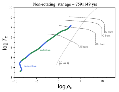
(a)

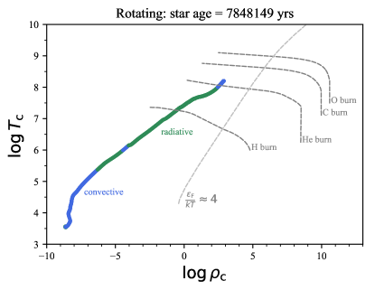
(b)

Figure 1: Structure of the 20 M_⊙ model in the temperature/density plane in core helium burning near the luminosity minimum for the non-rotating model (panel a) and for the rotating model (panel b). The blue regions are convective, the green regions, radiative. The dashed line corresponding to $\epsilon_{F}/(kT)\approx 4$ represents the non-degenerate/degenerate boundary. Note in both models the convective region around $10^{6}$ K that is separated from the outer convective envelope by a radiative region.

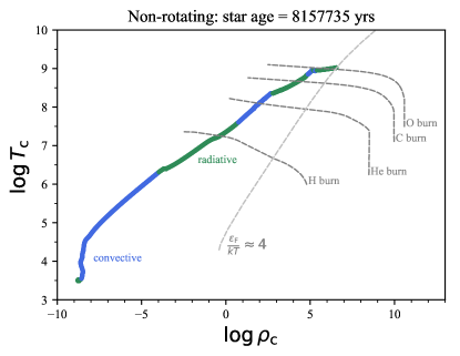
(a)

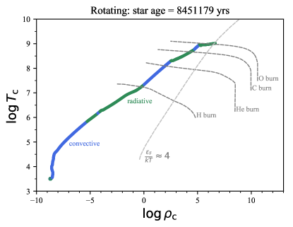
(b)

Figure 2: Structure of the 20 M_⊙ model in the temperature/density plane in the phase of off-center convective carbon burning for the non-rotating model (panel a) and for the rotating model (panel b). The blue regions are convective, the green regions, radiative.

3 Characteristic Frequencies

We estimated characteristic frequencies that might send acoustic signals to the surface. While it is conceivable that Betelgeuse is subject to opacity or nuclear–driven p–mode and g–mode pulsations and that this is the origin of the 420 day pulsation (§5), for this work we made estimates guided by the notion that the inner regions of a RSG will be characterized by turbulent noise associated with strong convection in the late stages of evolution as explored by Arnett & Meakin (2011), Smith & Arnett (2014), and Couch et al. (2015). Several works have employed these notions to explore the possibility that strong acoustic flux generated late in the evolution can lead to envelope expansion or even mass loss (Quataert & Shiode, 2012; Shiode & Quataert, 2014; Fuller, 2017a). Here we address earlier, gentler phases in an attempt to seek clues to the the evolutionary state of RSG prior to the final collapse.

We followed the techniques and methods outlined by Shiode & Quataert (2014) and Fuller (2017a) to determine convective and cutoff frequencies and dissipative processes. $MESA$ computes the distribution of convective velocities in convective regions. The distribution is not symmetric about the midpoint of typical convective zones, but nearly so. We thus estimated a characteristic angular frequency for the overturn of a convective eddy as

$$\omega_{conv}\approx\frac{v_{conv}}{H_{p}}$$ (1)

where $v_{conv}$ is the convective velocity in the middle of a convective core or shell, determined to be the half–way point in radius between boundaries of a shell or half the radius of a central convective core, and ${H_{p}}$ is the pressure scale height at the radial mid–point of the convective core or shell. A characteristic timescale associated with this frequency is thus

$$T_{conv}=\frac{2\pi}{\omega_{conv}}\approx\frac{2\pi H_{p}}{v_{conv}}.$$ (2)

We note that Fuller (2017a) defines the convective frequency to be $2\pi v_{conv}/2\alpha H_{p}$ with $\alpha=2$ and hence larger than adopted here and by Shiode & Quataert (2014) by a factor of $\pi/2$.

We must also consider the cutoff frequency in the outer envelope. If the frequency of a wave generated within the core is too low, that wave will not be able to propagate through the envelope. Shiode & Quataert (2014) estimated the cut–off frequency of the outer convective envelope as

$$\omega_{cut}\approx\frac{c_{s}}{H_{p}}$$ (3)

where $c_{s}$ is the sound speed and $H_{p}$ the pressure scale height in the envelope measured at 1/2 of the radius of the model. In order to propagate to the surface, $\omega_{conv}>\omega_{cut}$. While this prescription gives a useful guideline, we note that the cutoff frequency can be a rather sensitive function of position in the envelope. Figure 3 gives the distribution of $\omega_{cut}$ in the envelope of the non-rotating 20 M_⊙ model at the luminosity minimum and in the stage of carbon shell burning; the rotating models are virtually indistinguishable in this regard. In this figure, the X marks the frequency of $\omega_{cut}$ at the half-radius point. Horizontal lines correspond to the frequencies generated by various features, as presented below. The low frequencies generated in the outer envelope or the isolated H convective shell will not propagate, though large convective plumes may reach the surface. Frequencies generated by the helium-burning core or the later convective helium shell may not propagate. The frequencies estimated for the carbon-burning shell are expected to propagate through the envelope by this criterion. In the analysis below, we present the frequencies generated by these various features as a function of the mass of the stellar model and display them in comparison with $\omega_{cut}$ as computed by equation 3 at the half-radius point. The qualitative results for the lowest and highest frequencies are rather clear; the issue of the propagation of waves produced in the helium convective regions may be marginal. For the current discussion we ignore issues of wave dissipation; we return to this issue in §4.

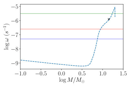
(a)

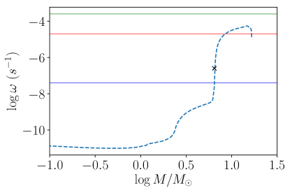
(b)

Figure 3: The wave propagation cutoff frequency given by equation 3 (dashed line) is given as a function of mass for the non-rotating 20 M_⊙ model in panel a at the minimum in luminosity at the base of the RSB (Figure 1) and in panel b in shell carbon burning (Figure 2). The X marks the cutoff frequency evaluated at half the radius of the star. In panel a, the blue line at $log~{}\omega\sim-7.3$ gives the frequency of the outer convective envelope, the red line at $log~{}\omega\sim-6.7$ gives the frequency generated by the inner convective hydrogen shell, and the green line at $log~{}\omega\sim-5.5$ gives the frequency generated in the helium core (see Figure 4). In panel b, the blue line at $log~{}\omega\sim-7.5$ gives the frequency of the outer convective envelope, the red line at $log~{}\omega\sim-4.7$ gives the frequency generated by the helium shell, and the green line at $log~{}\omega\sim-3.7$ gives the frequency generated in the carbon shell (see Figure 6).

Figure 4 gives the distribution of convective frequencies and the half-radius envelope cut-off frequency as a function of ZAMS mass at the point of minimum luminosity at the base of the RSB for the non–rotating models. These models are early in core helium burning. The outer convective envelope shows the characteristic timescale, $T\sim$ years, that is characteristic of the 420 day pulsation and slow overturn of the convective plumes. As illustrated in Figures 1 and 2, models of the type we are studying often have a deeper hydrogen convective shell at $T\sim 10^{6}$ K that is separated from the outer convective envelope by a radiative region. This deeper convective hydrogen–rich region has a characteristic timescale of $T\sim$ months. The timescale corresponding to the cut–off frequency varies from 20 to 70 days. Only the inner helium–burning convective core with a characteristic time of $T_{conv}\sim 20$ d might have the possibility to generate pressure waves that could propagate to the surface. The frequency of this mode varies by about 20% over the range of our models, too small to be seen easily on this log plot.

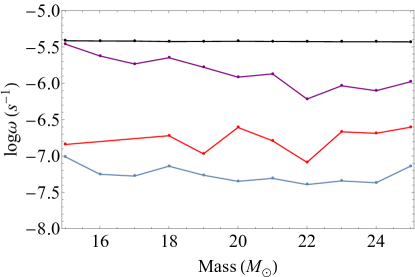
Figure 4: The distribution of convective frequencies and the half-radius envelope cut–off frequency as a function of ZAMS mass at the point of minimum luminosity at the base of the RSB for the non–rotating models. Similar convective structures are connected by the solid lines. The purple curve around $log~{}\omega\sim-6$ denotes the cut-off frequency, below which none of the characteristic convective frequencies are expected to propagate to the surface. The blue curve around $log~{}\omega\sim-7.3$ corresponds to the outer convective envelope with a characteristic period, $T_{conv}$, of years. The red curve around $log~{}\omega\sim-7$ corresponds to a separate convective shell with $T\sim 10^{6}$ K that has a period about 3 times less. Only the convection in the helium core with a frequency $log~{}\omega\sim-5.5$ denoted by the black line might be observable at the surface with an overturn time of $\sim$ 20 d.

Figure 5 gives the distribution of convective frequencies and the half-radius envelope cut-off frequency as a function of ZAMS mass at the point near where the rotational velocity is $\sim 15$ km s^-1 near the base of the RSB for rotating models (Wheeler et al., 2017). Figures 1 and 2 show that while there is some difference in the structure of the outer envelope in the rotating model, there is relatively little difference in the deeper interior. The outer convective envelope of the rotating model shows a characteristic period of about a year, similar to that in Figure 4, but somewhat shorter since the evolution is at a slightly earlier phase. The deeper convective hydrogen shell at $T\sim 10^{6}$ K has nearly the same period as in Figure 4 and very similar to that of the outer envelope. The inner helium–burning convective core again has a characteristic period of $\sim 20$ d, but so too does the cut-off frequency that does not show the increase in period with mass that characterized the cut-off frequency in Figure 4. Taken at face value, the models that formally match the observed rotation velocity might be expected to reveal no inner signals. In principle, the detection of such signals with a period of about 20 days might allow discrimination of non-rotating from rotating models early in the core helium–burning phase.

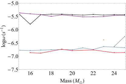
Figure 5: Similar to Figure 4 for the rotating models at the base of the RSB where they have rotational velocity $\sim 15$ km s^-1. The purple curve around $log~{}\omega\sim-5.5$ denotes the cut-off frequency. The blue curve around $log~{}\omega\sim-6.8$ corresponds to the outer convective envelope with a characteristic period of years. The red curve around $log~{}\omega\sim-6.8$ corresponds to the convective hydrogen shell at $T\sim 10^{6}$ K. Even the convection in the helium core with a frequency $log~{}\omega\sim-5.4$ and a period of $\sim$ 20 d denoted by the black line might not be observable at the surface.

Figure 6 gives the distribution of convective frequencies and the half-radius envelope cut–off frequency as a function of ZAMS mass at the carbon shell-burning phase for the non–rotating models. Here the structure of the convective regions is more complex. We have attempted to identify similar regions in each ZAMS mass but note that there are some models that do not display a particular structure when adjacent masses do (hence a missing “dot" in the figure) and others where a given structure is displayed by only a limited mass range. We have only attempted to capture regions of full convection and have neglected regions of semi–convection on the grounds that their slower overturn will lead to low frequencies and low power. The outer envelope again shows a period of years. The timescale corresponding to the cut–off frequency is about 70 days. The characteristic period of the separate hydrogen–rich convective shell with $T\sim 10^{6}$ K again has a period of months, is quite close to the cutoff frequency for many models, and is manifest for a restricted set of models, 17, 18, and 21. A principle feature of these models is the convective helium–burning shell with a period at about 10 d and the convective carbon–burning shell at about 1 d or less (both with significant variation with mass) that could, in principle, produce waves that propagate to the surface, indicating the presence of those structures. Model 19 has two inner convective regions with nearly the same frequency, one at $m_{r}=1.30$ M_⊙ and one at slightly higher frequency at $m_{r}=1.13$ M_⊙. Models 17 and 19 have an intermediate convective layer at about $m_{r}=2.5$ M_⊙, somewhat deeper than the helium convective shell and with somewhat higher frequency.

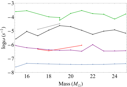
Figure 6: Similar to Figure 4 for carbon shell burning for the non–rotating models. The purple curve around $log~{}\omega\sim-6.2$ denotes the cut-off frequency. The blue curve around $log~{}\omega\sim-7.2$ corresponds to the outer convective envelope with a characteristic period of years. The red curve around $log~{}\omega\sim-6$ corresponds to the separate convective hydrogen shell with $T\sim 10^{6}$ K. The black curve around $log~{}\omega\sim-5$ corresponds to the helium–burning convective shell. The green curve around $log~{}\omega\sim-4$ corresponds to the carbon–burning shell. Intermediate convective structures are formed at some masses (gray curve). The convection in the deeper convective helium- and carbon-burning shells might generate gravity and pressure waves that propagate to the surface with periods of about 10 d and 1d, respectively.

Figure 7 gives the distribution of convective frequencies and the half-radius envelope cut–off frequency as a function of ZAMS mass at the carbon shell-burning phase for the rotating models. The outer envelope shows the characteristic period of years. The hydrogen shell at $T=10^{6}$ K appears only sporadically in the models but with characteristic period of months. The characteristic period of the convective helium shell is again about 10 d. The inner carbon shell has a period of a few tenths of a day. With the exception of the outer convective envelope, all the convective regions illustrated could, in principle, produce waves that propagate to the surface. As for the non–rotating models, the structure near carbon burning is expected to produce a more complex spectrum with generally higher frequencies than the models near the base of the giant branch.

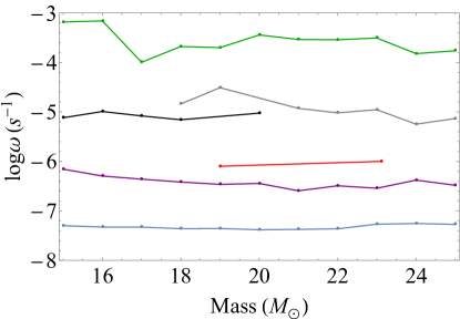
Figure 7: Similar to Figure 6 at carbon shell burning for the rotating models. The purple curve around $log~{}\omega\sim-6.2$ denotes the cut-off frequency. The blue curve around $log~{}\omega\sim-7.2$ corresponds to the outer convective envelope with a characteristic period of years. The red points correspond to the convective hydrogen shell at $T\sim 10^{6}$ K. The black and gray curves around $log~{}\omega\sim-5$ correspond to the convective helium–burning shell. The green curve at $log~{}\omega\sim-3$ to -4 corresponds to the carbon–burning shell. The convection in the convective helium– and carbon–burning shells might generate gravity and pressure waves that propagate to the surface with periods of about 10 d and 0.1 to 1 d, respectively. The intermediate hydrogen convective structures might also have potentially observable frequencies.

4 Detectability

Generating gravity waves in convective regions is one thing, getting a signal to the surface is quite another. There are several stages in the process as discussed by Quataert & Shiode (2012), Shiode & Quataert (2014) and Fuller (2017a). Only a fraction of the convective energy is converted to gravity waves that propagate in radiative regions where their frequency is less than the Brunt-Vaisala frequency. These waves must then pass through outer convective regions where they evanesce with a certain damping rate (Unno et al., 1989). Note that these outer convective regions can generate their own gravity waves. Eventually, the gravity waves will reach a position in the star at which their frequency exceeds the Lamb frequency, $\sqrt{\ell(\ell+1)}c_{s}/r$, where $c_{s}$ is the local sound speed and $\ell$ is the mode order. At that point, the waves will be converted to acoustic waves. In practice, this conversion occurs around the outer boundary of the helium core where the density and sound speed drop significantly. These acoustic waves will strengthen as they propagate down the density gradient into the outer envelope. If they develop into shocks or lose their energy to thermal diffusion, they will be dissipated and not reach the surface. There are a variety of other effects that must be taken into account, such as neutrino damping in the core, and wave reflections from composition boundaries in which the density gradient is steep and hence the WKB approximation breaks down.

Here we will address a few of the major factors, especially the efficiency of converting convective power into gravity waves and the thermal dissipation in the envelope. Following Shiode & Quataert (2014) and Fuller (2017a), we will only consider modes of angular frequency given by equation 1 and with $\ell=1$ since lower frequency waves tend to be more highly damped by shocks (but see the discussion on thermal diffusion which is less for low frequency; equation 12) and higher frequencies from a given source contain less power, and waves with larger values of $\ell$ both contain less power and are more strongly damped. Fuller (2017a) finds that the loss of power due to evanescence is a factor between 2 and 10. This is a significant factor, but small compared to other uncertainties. We omit this factor from our formal calculations, but note its role and return to a discussion of this factor in §4.4.2. The acoustic waves that might propagate to the surface have frequencies much higher than the envelope pulsation mode of 420 days or the longer envelope convective overturn time. These structures are effectively “frozen" on the timescales of the inner convective regions.

In the following discussion we focus on the non-rotating model with ZAMS mass of 20 M_⊙. This mass is the most likely value for Betelgeuse (but not, of course, for other RSG), and we find that rotation does not substantially affect the issues involved.

4.1 Convective Power

To estimate the possible detectability of the characteristic frequency from the convective noise, we first estimated the power associated with convective kinetic energy in each convective region as

$$L_{conv}\sim\frac{1}{2}\Delta M_{conv}v_{conv}^{2}T_{conv}^{-1}\sim\frac{1}{4\pi}\Delta M_{conv}\frac{v_{conv}^{3}}{H_{p}}$$ (4)

where $\Delta M_{conv}$ is the mass in the convective region. Following Cox & Giuli (1968) (§§14.2, 14.3, equations 14.113 and 14.114), a more rigorous estimate allowing for radiative losses yields

$$L_{conv}\approx 4\frac{dm}{dr}v_{conv}^{3},$$ (5)

which agrees with equation 4 within factors of a few.

Interestingly, for the RSG models we study here, these prescriptions give a value of $L_{conv}$ that is smaller than the value computed directly by $MESA$ by a factor $\sim 100$. The estimates in equations 4 and 4 assumed that a factor $c_{p}\rho T/P$ was of order unity. Closer inspection revealed that not to be the case. This factor averages of order 10 to 20 both at the base of the RSB and in carbon shell burning and spikes to close to 50 at certain locations in the latter case. Figure 8 shows the convective luminosity as a function of mass estimated by the three methods, equation 4 and equation 5, using the values of $v_{conv}$, $H_{P}$, and $dm/dr$ computed by $MESA$, and the $MESA$ value for $L_{conv}$ in core helium burning at the base of the RSB and in carbon shell burning for the model of 20 M_⊙. For the subsequent discussion, we employ the $MESA$ value for $L_{conv}$. Figure 8 also gives the total luminosity at the photosphere for the model at the base of the RSB and in carbon shell burning. Note that the convective luminosity in the helium-burning core is less than the radiated luminosity while that in the helium-burning shell is comparable to the radiated luminosity. The convective luminosity in the carbon-burning shell substantially exceeds the radiated luminosity. For illustration, we take the value of the convective luminosity at the radial midpoint in each region in the following discussion.

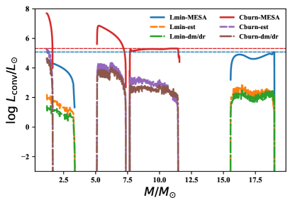
Figure 8: Three estimates of the convective luminosity are given as a function of mass for the 20 M_⊙ non-rotating model. The solid lines present the parameter $L_{conv}$ computed by $MESA$ using mixing-length theory; blue represents core helium burning near the base of the RSB, red the phase of shell carbon burning. The lower estimates that roughly agree with one another given by the dashed lines are based on equations 4 (orange and purple for core helium burning and carbon shell burning, respectively) and 5 (green and brown for core helium burning and carbon shell burning, respectively) employing the value of $v_{conv}$, $H_{P}$ and $dm/dr$ computed by $MESA$. The horizontal dashed lines (blue for the base of the RSB and red for carbon shell burning) indicate the level of the total luminosity radiated at the photosphere.

Table 1 gives the period, $T_{conv}=2\pi/\omega_{conv}$, and convective luminosity for a representative sample of convective zones for the non-rotating 20 M_⊙ model in order of increasing depth in the model. Only modes with frequencies comparable to or above the envelope cut–off frequency are presented. Goldreich & Kumar (1990) argued that the efficiency of conversion of convective energy into the energy of gravity waves is approximately $\mathcal{M}$, the mean Mach number in the convective region. Lecoanet & Quataert (2013) estimate that the efficiency might be higher, scaling as $\mathcal{M}^{5/8}$. Table 1 also gives estimated power in gravity waves for this model using these two efficiency factors.

Taking the results of Table 1 at face value, the inner convection could deliver appreciable power to the surface of the star. The helium core could produce $\sim 10^{36}$ erg s^-1 and the convective carbon shell phase up to $\sim 10^{38}$ erg s^-1, especially if the convection is efficient in producing acoustic waves. Such changes might produce interesting effects. At this point, we have not yet accounted for various efficiency and dissipation factors. More important, to be significant in an asteroseismic context, the critical factor is not an increment in power radiated, but whether the acoustic waves can perturb the surface luminosity in a manner that carries information about the deep convective layers.

Table 1: Estimated Gravity-Wave Power Generated at the Radial Midpoint in Convective Regions for the Non-rotating 20 M_⊙ Model.

	$T_{conv}$	$L_{conv}$	$\mathcal{M}$	$L_{conv}$$\mathcal{M}$	$L_{conv}$$\mathcal{M}^{5/8}$
	days	$10^{36}$	$10^{-4}$	$10^{36}$	$10^{36}$
		erg s-1		erg s-1	erg s-1
$L_{min}$
He core	21.1	133	2.04	0.0271	0.656
C burn
He shell	13.8	3470	24.6	8.55	81.4
C shell	0.14	7620	1.25	0.953	27.7

4.2 Wave Amplitudes

The acoustic waves gain in amplitude as they run down density gradients, especially the sharp gradient that marks the passage from the outer helium core to the hydrogen envelope. Defining $\xi$ to be the amplitude or radial displacement of the wave, the luminosity of the wave can be written

$$L_{wave}=4\pi r^{2}\rho(\xi\omega)^{2}c_{s}$$ (6)

so that with wavenumber $k=\omega/c_{s}$ the dimensionless quantity $k\xi$, the displacement relative to the wavelength, can be written

$$k\xi=\left(\frac{L_{wave}}{4\pi r^{2}\rho c_{s}^{3}}\right)^{1/2}\approx 8.9\times 10^{-5}\left(\frac{L_{wave,36}}{r_{11}^{2}\rho c_{s,7}^{3}}\right)^{1/2}$$ (7)

where $L_{wave,36}$ is the wave amplitude in units of $10^{36}$ erg s^-1, a typical luminosity for the weak waves we consider here (Table 1), $r_{11}$ is the radius in units of $10^{11}$ cm that is characteristic of the helium core, and $c_{s,7}$ is the sound speed in units of $10^{7}$ cm s^-1. Quataert & Shiode (2012) give a similar expression. This shows that the initial amplitude of the waves is small.

Figure 9 shows the relative displacement, $k\xi$, versus radius for waves generated in the convective helium core when near the base of the RSB and in the convective helium and carbon shells when in the carbon shell-burning phase for the non-rotating 20 M_⊙  model. In the outer part of the helium core, $r_{11}\sim 4$, the density is near 1 g cm^-3, and the sound speed is $c_{s,7}\sim 10$. The value of $k\xi$ is of order $10^{-6}$ for all models. From this low value, the outer edge of the model corresponding to the base of the RBG is reached before $k\xi$ reaches unity. In the carbon shell-burning phase, $k\xi$ exceeds unity in the outer reaches of the model.

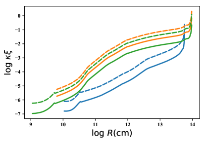
Figure 9: The relative displacement, $k\xi$, (equation 7) is given as a function of radius for gravity waves emitted from the convective helium-burning core at the base of the RSB (blue) and from the carbon (green) and helium (orange) convective burning shells in carbon shell burning for the non-rotating 20 M_⊙ model. The corresponding gravity-wave luminosities in each case are given in Table 1; values of $k\xi$ corresponding to the convective luminosity reduced by the Mach number, $L_{conv}$$\mathcal{M}$, are given by the solid lines and the dashed lines correspond to $L_{conv}$$\mathcal{M}^{5/8}$.

4.3 Modulation of Surface Luminosity

The modulation of the luminosity due to linear adiabatic modulation by acoustic waves is very roughly given by (Unno et al., 1989)

$$\frac{|\Delta L|}{L}\sim k\xi.$$ (8)

The perturbation of the luminosity radiated at the surface due to perturbations in the temperature, density, and surface area can be approximated by evaluating equation 7 at the location in the envelope where $\omega\tau_{therm}\sim 1$, where $\tau_{therm}$ is the local thermal timescale,

$$\tau_{therm}=\frac{4\pi r^{2}H_{p}\rho c_{P}T}{L}$$ (9)

and where $c_{P}$ is the specific heat at constant pressure and $L$ is the radiated flux (Pfahl et al., 2008; Fuller, 2017b).

We sought to evaluate equation 8 by computing $\omega\tau_{therm}$ as a function of $r$ for a given frequency of interest as given in Table 2 and then evaluating equation 7 at that radius. The perturbation to the luminosity in magnitudes due to the modulation by the convective noise would then be

$$\delta m=\left|-2.5{\rm log}\left(\frac{L_{rad}+|\Delta L_{surf}|}{L_{rad}}\right)\right|\approx 1.1\frac{|\Delta L_{surf}|}{L_{rad}}$$ (10)

where $|\Delta L_{surf}|<<L_{rad}$ is the absolute value of our estimate of the observable perturbation of the luminosity at the surface.

Table 2: Frequencies¹ Employed to Compute Wave Amplitudes and Damping Masses

Model Mass	Helium Core	Helium Shell	Carbon Shell
15	$3.5\times 10^{-6}$	$5.3\times 10^{-6}$	$5.2\times 10^{-4}$
20	$3.8\times 10^{-6}$	$2.0\times 10^{-5}$	$1.8\times 10^{-4}$
25	$3.7\times 10^{-6}$	$6.9\times 10^{-6}$	$1.7\times 10^{-4}$
1 in units of $s^{-1}$

In practice, we found this prescription difficult to implement in a straightforward manner. For the non-rotating 20 M_⊙ model at the base of the RSB, we found that $\omega\tau_{therm}=1$ only very close to the surface. For the model in carbon shell burning, $\omega\tau_{therm}$ did not reach unity with the resolution of the current model. The implication is that inasmuch as $\omega\tau_{therm}$ nears unity, it is at a radius that is essentially equal to the outer radius of the model. We can then evaluate Equation 8 at the outer radius of the model. For the models we consider here, typical values for the density and sound speed in the outer layers are $10^{-8}$ g cm^-3 and $10^{6}$ cm $s^{-1}$ so we can estimate

$$\frac{|\Delta L_{surf}|}{L}\sim 2.8\times 10^{-2}\left(\frac{L_{wave,36}}{R_{14}^{2}\rho_{-8}c_{s,6}^{3}}\right)^{1/2}$$ (11)

For the non-rotating 20 M_⊙ model, the ratio of the amplitude of the perturbed luminosity to the total luminosity (neglecting any subsequent damping between the source and the surface for now) estimated in this way is given in Table 3 (the parameter $d_{a}$ is discussed below, equation 14), assuming all the factors in the denominator of equation 11 are unity. The estimated variation in magnitudes would be larger than $\Delta L_{surf}/L$ by about 10%, according to equation 10. At this point, the results are encouraging, ranging from potential perturbations of order several millimagnitudes up to a few tenths of a magnitude, well within the range of astronomical detection.

Table 3: Estimated Perturbation of the Surface Luminosity, $\frac{|\Delta L_{surf}|}{L}$, by Acoustic Waves for the Non-rotating 20 M_⊙ Model.

	$L_{conv}$$\mathcal{M}$	$L_{conv}$$\mathcal{M}^{5/8}$	${\rm log}~{}d_{a}$
$L_{min}$
He core	0.0047	0.023	1.6
C burn
He shell	0.083	0.26	220
C shell	0.028	0.15	22,000

4.4 Wave Dissipation Processes

Even if the wave powers estimated in Table 1 are appropriate, the acoustic waves have yet another gauntlet to run before imparting any perturbation to the surface luminosity as estimated in Table 3. They must avoid dissipation in the envelope either by growing to non-linear amplitudes and becoming shocks or losing their energy to thermal diffusion.

4.4.1 Shock dissipation

In our models, the density typically drops from $\rho\sim 10$ g cm^-3 in the outer helium envelope to $\rho\sim 10^{-6}$ g cm^-3 at the base of the hydrogen envelope. For the latter density, equation 7 gives $k\xi\sim 0.1$, suggesting that these relatively weak waves may escape shock formation at that point. The density continues to decline in the hydrogen envelope, but the radius increases so there is a tradeoff that helps preserve the waves.

Figure 9 gives the quantitative prediction of the profile of $k\xi$ for characteristic phases of the 20 M_⊙ model. The relative displacement remains less than $10^{-2}$ until the outermost layers. This suggests that shocks will not necessarily form already at the base of the hydrogen envelope. According to Ro & Matzner (2017), shocks may form even more robustly than we have estimated here by examining the behavior of $k\xi$. This will exacerbate the likelihood that gravity waves from the carbon-burning shell will dissipate in shocks at the base of the outer convective envelope, but might still mean that the weak waves from core helium burning survive that process.

4.4.2 Thermal Dissipation

The other factor that imperils the propagation of the waves is the dissipation by thermal diffusion (Quataert & Shiode, 2012; Shiode & Quataert, 2014). Fuller (2017a) expresses this as a damping mass

$$M_{damp}=\frac{3\pi\rho^{3}r^{2}c_{s}^{3}c_{p}\kappa}{4\sigma T^{3}\omega^{2}}\approx 7\times 10^{5}M_{\rm\odot}\frac{\rho_{-6}^{3}r_{12}^{2}c_{s,7}^{3}}{T_{4}^{3}\omega_{-6}^{2}},$$ (12)

where $c_{p}$ is the specific heat at constant pressure, $\kappa\sim 0.4$ cm^-2 g^-1 is the opacity, $\sigma$ is the Stefan-Boltzmann constant, $r_{12}$ is the radius in units of $10^{12}$ cm that is more characteristic of the hydrogen envelope, $\rho_{-6}$ is the density in units of $10^{-6}$ g cm^-3, $T_{4}$ is the temperature in units of $10^{4}$ K, and $\omega_{-6}$ is the frequency in units of $10^{-6}$ s^-1. This damping mass is an especially sensitive function of the density. If the density plummets to a sufficiently low value in the hydrogen envelope, the wave energy will be rapidly dissipated. The resulting heating can cause the envelope to expand (Fuller, 2017a) or even dynamically eject some of the envelope (Shiode & Quataert, 2014). There is an implied threshold such that once the waves begin to dissipate and expand the envelope, the envelope density will decrease, increasing the tendency for the waves to dissipate.

The weak waves we consider here may or may not dissipate. To check this, we have examined the density structure and hence the variation of $M_{damp}$ for models in which the heating from dissipation is ignored, leading to relatively large envelope densities. Figures 10 and 11 give the distribution of the damping mass as a function of the mass of the model (that is subject to mass loss) at the given stage of evolution for our models of 15 and 20 M_⊙, respectively, for core helium burning near the base of the RSB and in the stage of the first off-center convective shell carbon-burning for non-rotating models. The corresponding frequencies are given in Table 2. We also computed a 25 M_⊙ model, but had problems with model convergence with the default mass loss. Halving the “Dutch" mass-loss rate from $\eta=0.8$ to $\eta=0.4$ yielded a converged model, but at the expense of a somewhat different model prescription. We show the results of this model in Figure 12.

The models illustrated in Figures 10, 11, and 12 show that in the unlikely circumstance that a star is near the base of the RGB at the epoch of observation, the damping masses in the envelope remain substantially larger than the envelope mass throughout the bulk of the envelope. These waves may make it to near the surface. These figures also show that the low-frequency waves of shell helium burning may escape diffusive damping in the envelope. For the 15 M_⊙ model in the stage of shell carbon burning, $M_{damp}$ for waves from the helium shell remains well above 1 M_⊙ to the outer reaches of the envelope. The damping mass plummets there, a point we return to below. The 20 M_⊙ model shows a peak in $M_{damp}$ for the helium shell in the outer portions of the envelope, but $M_{damp}$ is substantially less than 1 M_⊙ over much of the envelope. The 25 M_⊙ model shows that $M_{damp}$ for the helium shell exceeds the mass of the envelope through much of the envelope, but with a minimum that dips to close to the envelope mass. Acoustic waves from a star that reflected this model’s properties might make it to the surface. This model had a decreased rate of mass loss compared to the lower-mass models. Whether adjustment of mass loss or other model parameters would yield more dissipation in the 25 M_⊙ or less in the 20 M_⊙ model requires further investigation. For all three models, the high-frequency waves from carbon shell burning are strongly damped in the extended, dilute envelope corresponding to the tip of the RGB and are unlikely to make it to the surface despite the greater power generated compared to the helium shell.

It is also important to keep in mind that while we have estimated characteristic frequencies, the inner convective regions will each produce a broad spectrum of acoustic frequencies. Some of these will be more prone to dissipation, some less so.

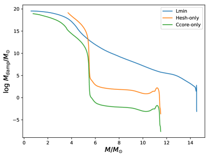
Figure 10: The distribution of the damping mass $M_{damp}$ from equation 12 at two evolutionary stages for the non-rotating model of 15 M_⊙. Blue corresponds to the model in convective core helium burning at the base of the RGB, yellow to the helium burning shell during the first stage of off-center convective carbon burning and green to that carbon-burning shell.

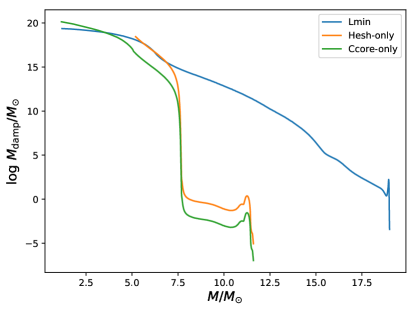
Figure 11: Similar to figure 10, but for the non-rotating model of 20 M_⊙.

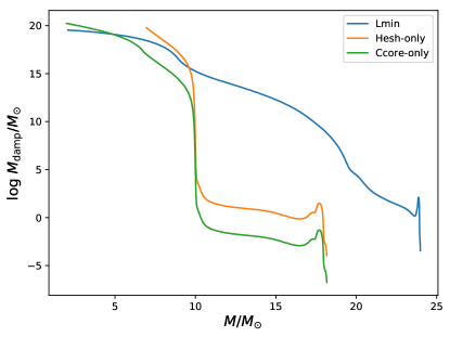
Figure 12: Similar to figure 10, but for the non-rotating model of 25 M_⊙.

Another perspective on thermal dissipation can be obtained by taking

$$\frac{dL}{m}=-\frac{L}{M_{damp}}$$ (13)

(Fuller, 2017a), so we can write

$$ln\frac{L}{L_{0}}=-\int\frac{dm}{M_{damp}}$$ (14)

where $L_{0}$ is the generated acoustic power and $L$ is evaluated at a given mass coordinate. The energy in the waves is thus dissipated by a factor $exp(-2d_{a})$, and the amplitude of the waves by a factor $exp(-d_{a})$. Figure 13 gives the quantity, $2d_{a}$, as a function of mass for the non-rotating 20 M_⊙ model, again in core helium burning at the base of the RGB and in the carbon shell-burning phase. This attenuation is less than unity for most of the core helium burning model until the very outer portions of the envelope where it might somewhat exceed unity in the amplitude, consistent with Figure 11 (neglecting the very outer spike for now). Table 3 also gives the log of the amplitude of the dissipation factor, $d_{a}$, for three relevant cases evaluated in the outer envelope but prior to the very outer spike in $M_{damp}$ for the non-rotating 20 M_⊙ model. While the small amplitudes of the acoustic waves from the early core helium burning may be dissipated by a factor of order 10, the waves from both the helium and carbon shells in the later phases are severely dissipated in the 20 M_⊙ model, even before encountering the spike in $M_{damp}$. We note from Figures 10 and 12 that the dissipation of acoustic waves from the helium-burning shell is especially severe for the 20 M_⊙ model and that the attenuation for those waves may be less for other masses.

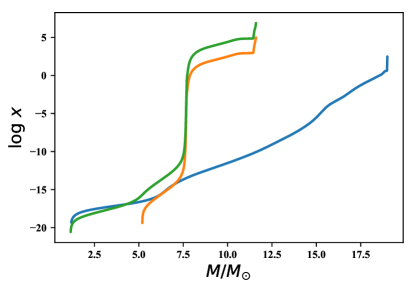
Figure 13: The quantity $x=\int\frac{dm}{M_{damp}}\equiv 2d_{a}$ is presented as a function of mass for the non-rotating 20 M_⊙ model for the convective helium core at the base of the RGB (blue line), the helium shell in carbon shell burning (orange line) and the carbon shell (green line).

4.4.3 Effects of Outer Envelope

To this point, we have ignored the behavior of the wave amplitude, the damping mass, and the attenuation factor in the very outermost layers, where Figures 10, 11, and 12, all show a peak and then a steep drop and Figures 9 and 13 show a spike for all three cases illustrated. Concerned that this was some numerical issue, we examined this outer structure more carefully. To this end, we present in Figure 14 a plot of $M_{damp}$ as a function of optical depth from the surface for the same three cases represented in Figure 13. This shows that the peak in $M_{damp}$ in Figures 10, 11, and 12 occurs at large optical depth, $\tau\sim 10^{4.5}$, not in the outer atmosphere. For reference, the small outer ledge in $M_{damp}$ that can be discerned in Figures 10 through 12 occurs at $\tau\sim 20$.

The outer peak in $M_{damp}$ typically occurs at a mass depth of about 1 M_⊙ from the surface. The damping mass rapidly plummets outward from the peak. The outer steep declines in $M_{damp}$ in Figures 10, 11, and 12 and the outer spikes in Figures 9 and 13 are real and ubiquitous. These features are associated with the strong negative gradient in $\rho$ (see equation 12) in the outer, but still optically-thick layers. This implies that even if acoustic waves reached the location of the outer peak in $M_{damp}$, they are likely to thermally dissipate before reaching the surface.

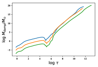
Figure 14: The damping mass for thermal diffusion at a given radius is given as function of optical depth from that position to the surface for the non-rotating model of 20 M_⊙ for the convective helium core at the base of the RGB (blue line), the helium shell in carbon shell burning (orange line) and the carbon shell (green line).

5 Discussion

There is potential to determine the mass, the rotation, the internal structure, and the evolutionary state of Betelgeuse and other red supergiants, if any faint, fast, acoustic perturbations could be detected. By the time the models have reached the tip of the giant branch, the outer, extended convective envelope is well established, but the inner structure is quite variable, with convective regions developing and vanishing and with different configurations at different times for different ZAMS masses. That Betelgeuse is in some phase of core helium burning is most probable, but later stages are not precluded. The inner convective regions should generate gravity waves that convert to acoustic waves with characteristic periods of 20 days in core helium burning, 10 days in helium shell burning, and 0.1 to 1 day in shell carbon burning.

Whereas Shiode & Quataert (2014) and Fuller (2017a) focused on very late stages where acoustic flux could be strong enough to drive envelope expansion or mass loss, here we sought conditions where acoustic waves might give some diagnostic of the inner properties of red supergiants like Betelgeuse. Shiode & Quataert (2014) and Fuller (2017a) caution that dissipation may prevent any acoustic waves from propagating to the surface. Although our models in this survey are a sparse sample of the evolutionary states, we largely confirm these pessimistic results. We find that acoustic waves may propagate to near the surface, avoiding both shock and diffusive dissipation relatively early in core helium burning with a luminosity amplitude of about a millimagnitude. By the time the models are in shell carbon burning, the signals leaving the helium and carbon shells have more power, but shock and especially thermal dissipation and attenuation cause damping in the outer convective envelope. This damping may be less for acoustic waves generated by the helium-burning shells in the the 15 M_⊙ and 25 M_⊙ models than for the 20 M_⊙ model, but it is severe in all the models for the waves from the carbon-burning shell.

In all the models we investigated, the rapid decline in density in the outermost, but still optically thick, layers, seemed to provide a last blockade against observable perturbations to the surface luminosity, dissipating any impinging acoustic wave by some combination of thermal dissipation and shock formation. Other factors are neutrino losses in the core or wave reflection, both of which we have ignored here.

We have presented rudimentary theory here that is subject to manifest uncertainties. Betelgeuse and most other massive RSG are most likely to be in mid to late core helium burning – the longest-lived phase after the main sequence – for which we predict little observable signal. On the other hand if Betelgeuse were in core silicon burning with only days to live, there would be no time for waves to reach the surface and hence little to see (Fuller, 2017a). Absence of evidence does not mean things might not get exciting very quickly.

It would be interesting to do a more careful study of structure while near the tip of the RSB. Of interest would be to establish the phase of core helium burning when evidence for that core convection first becomes observable in principle, with the convective frequency greater than the envelope cutoff frequency and to probe the evolving structure at and beyond core helium burning. The nature of the inner convective regions, their characteristic frequencies and power, and how they vary in time, require a dedicated study. We have not explored basic model sensitivity to issues like mixing length, overshoot, etc. We have done a basic exploration of the effects of rotation and associated mixing. Taking the possible effects of magnetic dynamos into account would add more complexity, but is within the capabilities of $MESA$. Even if acoustic wave perturbations cannot be observed directly, there may be some observable change in the structure of the outer envelope, its radius or its mass loss.

As mentioned in the Introduction, another potentially important constraint on Betelguese specifically is the observed 420 day pulsation mode. The pulsation period for convective envelopes scales as $P\propto R^{2}/M$ (Gough et al. 1965), so the period provides an important independent constraint on $R$ and $M$, depending on the proportionality constant. From the models of Heger et al. (1997), the envelope pulsation of Betelgeuse is most likely to correspond to a first overtone. For its mass and luminosity, the fundamental period for Betelgeuse would be several times larger than the observed period. In these models, the pulsation grows to a non-linear limit and then has the potential to expel a super wind (Yoon & Cantiello, 2010). Betelgeuse is not doing that. It remains of great interest to try to establish the conditions, that may depend on rotation, magnetic fields, and whether a companion has been ingested, that will yield a stable non-linear pulsation with the observed period.

Shiode & Quataert (2014) and Fuller (2017a) have argued that dissipation of acoustic waves in the envelope may lead to expansion of the envelope and mass loss of various intensities. There is evidence that Betelgeuse has a region of extended material out to perhaps 10 stellar radii beyond the photosphere (Kervella et al., 2011) and that upward and downward flows extend into that material (Ohnaka et al., 2011). Dessart et al. (2017) argue that this material may routinely affect the breakout properties of a supernova shock. It is possible that this outer, dynamical shell is the result of dissipation of acoustic energy from the inner convective regions. If this is so, then it may be that there is no asteroseismological signal to be seen from Betelgeuse because the inevitable waves have been dissipated to expand the envelope.

On the other hand, it may be that the propagation of acoustic waves is more complex than has yet been explored. For instance, there may be percolation properties whereby outgoing acoustic waves selectively permeate cooler, denser, down-flowing plumes on their inward journey. Even if acoustic waves percolate, their effect on the surface might average out over the surface. Perhaps individual surface plumes would need to be studied for their asteroseismological properties.

We have treated the acoustic flux as if it had a single frequency from a single convective region, but every convective region will emit a spectrum of waves; perhaps some wavelengths are more penetrating that others. Another possibility might be to examine the surface properties in different wavelengths where the opacity is less (E. Levesque, private communication, 2018).

We have also seen suggestions that some masses may be more amenable to propagating acoustic waves than others. If, at some masses, one could discern acoustic perturbations from early and later core or shell helium burning, that stage of helium burning could be diagnosed.

It may very well be that there are no acoustic signals from the inner convective structure of RSG that reach the surface yielding clues to the inner structure and hence nothing to observe. Yet detection of such perturbations could provide a rich new way to probe the inner structure of supernova progenitors. Any detection would require an immense amount of work to quantitatively interpret the data – we have barely scratched model parameter space here – but it seems a shame not to try.

References

- Aerts (2015) Aerts, C. 2015, Astronomische Nachrichten, 336, 477
- Arnett & Meakin (2011) Arnett, W. D., & Meakin, C. 2011, ApJ, 733, 78
- Couch et al. (2015) Couch, S. M., Chatzopoulos, E., Arnett, W. D., & Timmes, F. X. 2015, ApJL, 808, L21
- Cox & Giuli (1968) Cox, J. P., & Giuli, R. T. 1968, Principles of stellar structure, by J.P. Cox and R. T. Giuli. New York: Gordon and Breach, 1968,
- Dessart et al. (2017) Dessart, L., Hillier, D. J., & Audit, E. 2017, arXiv:1704.01697
- Dolan et al. (2016) Dolan, M. M., Mathews, G. J., Lam, D. D., et al. 2016, ApJ, 819, 7
- Dupree et al. (1987) Dupree, A. K., Baliunas, S. L., Hartmann, L., et al. 1987, ApJL, 317, L85
- Fuller (2017a) Fuller, J. 2017a, MNRAS, 470, 1642
- Fuller (2017b) Fuller, J. 2017b, MNRAS, 472, 1538
- Goldreich & Kumar (1990) Goldreich, P., & Kumar, P. 1990, ApJ, 363, 694
- Gough et al. (1965) Gough, D. O., Ostriker, J. P., & Stobie, R. S. 1965, ApJ, 142, 1649
- Haubois et al. (2009) Haubois, X., Perrin, G., Lacour, S., et al. 2009, A&A, 508, 923
- Harper et al. (2008) Harper, G. M., Brown, A., & Guinan, E. F. 2008, AJ, 135, 1430
- Harper et al. (2017) Harper, G. M., Brown, A., Guinan, E. F., et al. 2017, AJ, 154, 11
- Kervella et al. (2011) Kervella, P., Perrin, G., Chiavassa, A., et al. 2011, A&A, 531, A117
- Kervella et al. (2018) Kervella, P., Decin, L., Richards, A. M. S., et al. 2018, A&A, 609, A67
- Lecoanet & Quataert (2013) Lecoanet, D., & Quataert, E. 2013, MNRAS, 430, 2363
- Montargès et al. (2017) Montargès, M., Chiavassa, A., Kervella, P., et al. 2017, A&A, 605, A108
- Ohnaka et al. (2011) Ohnaka, K., Weigelt, G., Millour, F., et al. 2011, A&A, 529, A163
- Paxton et al. (2011) Paxton, B., Bildsten, L., Dotter, A., et al. 2011, ApJS, 192, 3
- Paxton et al. (2013) Paxton, B., Cantiello, M., Arras, P., et al. 2013, ApJS, 208, 4
- Paxton et al. (2015) Paxton, B., Marchant, P., Schwab, J., et al. 2015, ApJS, 220, 15
- Pfahl et al. (2008) Pfahl, E., Arras, P., & Paxton, B. 2008, ApJ, 679, 783-796
- Quataert & Shiode (2012) Quataert, E., & Shiode, J. 2012, MNRAS, 423, L92
- Ro & Matzner (2017) Ro, S., & Matzner, C. D. 2017, ApJ, 841, 9
- Shiode & Quataert (2014) Shiode, J. H., & Quataert, E. 2014, ApJ, 780, 96
- Smith & Arnett (2014) Smith, N., & Arnett, W. D. 2014, ApJ, 785, 82
- Wheeler et al. (2015) Wheeler, J. C., Kagan, D., & Chatzopoulos, E. 2015, ApJ, 799, 85
- Wheeler et al. (2017) Wheeler, J. C., Nance, S., Diaz, M., et al. 2017, MNRAS, 465, 2654
- Unno et al. (1989) Unno, W., Osaki, Y., Ando, H., Saio, H., & Shibahashi, H. 1989, Nonradial oscillations of stars, Tokyo: University of Tokyo Press, 1989, 2nd ed.
- Decin et al. (2012) Decin, L., Cox, N. L. J., Royer, P., et al. 2012, A&A, 548, A113
- de Mink et al. (2014) de Mink, S. E., Sana, H., Langer, N., Izzard, R. G., & Schneider, F. R. N. 2014, ApJ, 782, 7
- Yoon & Cantiello (2010) Yoon, S.-C., & Cantiello, M. 2010, ApJL, 717, L62