Reversibility vs local creation/destruction

Abstract.

Consider a network that evolves reversibly, according to nearest neighbours interactions. Can its dynamics create/destroy nodes? On the one hand, since the nodes are the principal carriers of information, it seems that they cannot be destroyed without jeopardising bijectivity. On the other hand, there are plenty of global functions from graphs to graphs that are non-vertex-preserving and bijective. The question has been answered negatively—in three different ways. Yet, in this paper we do obtain reversible local node creation/destruction—in three relaxed settings, whose equivalence we prove for robustness. We motivate our work both by theoretical computer science considerations (reversible computing, cellular automata extensions) and theoretical physics concerns (basic formalisms for discrete quantum gravity).

1. Outline

The question. Consider a network that evolves reversibly, according to nearest neighbours interactions. Can its dynamics create/destroy nodes?

Issue 1. Consider a network that evolves according to nearest neighbours interactions only. This means that the same, local causes must produce the same, local effects. If the neighbourhood of a node $u$ looks the same as that of a node $v$, then the same must happen at $u$ and $v$.
Therefore the names of the nodes must be irrelevant to the dynamics. By far the most natural way to formalize this invariance under isomorphisms is as follows. Let $F$ be the function from graphs to graphs that captures the time evolution; we require that for any renaming $R$, $F\circ R=R\circ F$. But it turns out that this commutation condition forbids node creation, even in the absence any reversibility condition—as proven in [1]. Intuitively, say that a node $u\in G$ infants a node $u^{\prime}\in G^{\prime}$ through $F$, and consider an $R$ that maps $u^{\prime}$ into some fresh $v^{\prime}$. Then $F(RG)=F(G)$, which has no $v^{\prime}$, differs from $RF(G)$, which has a $v^{\prime}$.

Issue 2. The above issue can be fixed by asking that new names be constructed from the locally available ones (e.g. $u^{\prime}$ from $u$), and that renaming available names (e.g. $u$ into $v$) through $R$ leads to renaming constructed ones ($u^{\prime}$ into $v^{\prime}$) through $R^{\prime}$. Then invariance under isomorphisms is formalized by requiring that for any renaming $R$, there exists $R^{\prime}$, such that $F\circ R=R^{\prime}\circ F$. But it turns out that this conjugation condition, taken together with reversibility, still forbids node creation, as proven in [4]. Intuitively, say that a node $u$ infants two nodes $u.l$ and $u.r$. Then $F^{-1}$ should merge these back into a single node $u$. However, we expect $F^{-1}$ to have the same conjugation property that for any renaming $S$, there exists $S^{\prime}$, such that $F^{-1}\circ S=S^{\prime}\circ F^{-1}$. Consider an $S$ that leaves $u.l$ unchanged, but renames $u.r$ into some fresh $v^{\prime}$. What should $S^{\prime}$ do upon $u$? Generally speaking, node creation between $G$ and $F(G)$ augments the naming space and endangers the bijectivity that should hold between $\{RG\}$ the set of renamings of $G$ and $\{RF(G)\}$ the set of renamings of $F(G)$.

Issue 3. Both the above no-go theorems rely on naming issues. In order to bypass them, one may drop names altogether, and work with graphs modulo isomorphisms. Doing this however is terribly inconvenient. Basic statements such as “the neighbourhood of $u$ determines what will happen at $u$”—needed to formalize the fact the network evolves according to nearest-neighbours interactions—are no longer possible if we cannot speak of $u$.
Still, because these are networks and not mere graphs, we can designate a node relative to another by giving a path from one to the other (the successive ports that lead to it). It then suffices to have one privileged pointed vertex acting as the origin, to be able to designate any vertex relative to it. Then, the invariance under isomorphisms is almost trivial, as nodes have no name. All we need is to enforce invariance under shifting the origin. If $X_{u}$ stands for $X$ with its origin shifted along path $u$, then there must exist some successor function $R_{X}:V(X)\longrightarrow V(F(X))$ such that $F(X_{u})=F(X)_{R_{X}(u)}$. But it turns out that this even milder condition, taken together with reversibility, again forbids node creation but for a finite number of graphs—as was proven in [7].
Intuitively, node creation between $X$ and $F(X)$ augments the number of ways in which the graph can be pointed at. This again endangers the bijectivity that should hold between the sets of shifts $\{X_{u}\}_{u\in X}$ and $\{F(X)\}_{u^{\prime}\in F(X}$.

Three solutions and a plan. In [17], Hasslacher and Meyer describe a wonderful example of a nearest-neighbours driven dynamics, which exhibits a rather surprising thermodynamical behaviour in the long-run. This toy example is non-vertex-preserving, but also reversible, in some sense which is left informal.
The most direct approach to formalizing the HM example and its properties, is to work with pointed graphs modulo just when they are useful, e.g. for stating causality, and to drop the pointer everywhen else, e.g. for stating reversibility. This relaxed setting reconciles reversibility and local creation/destruction—it can be thought of as a direct response to Issue 3. Section 4 presents this solution.
A second approach is to simulate the HM example with a strictly reversible, vertex-preserving dynamics, where each ‘visible’ node of the network is equipped with its own reservoir of ‘invisible’ nodes—in which it can tap in order to infant an visible node. The obtained relaxed setting thus circumvents the above three issues. Section 5 presents this solution.
A third approach is to work with standard, named graphs. Remarkably it turns out that naming our nodes within the algebra of variables over everywhere-infinite binary trees directly resolves Issue 2. Section 6 presents this solution.
The question of reversibility versus local creation/destruction, is thus, to some extent, formalism-dependent. Fortunately, we were able to prove the three proposed relaxed settings are equivalent, as synthesized in Section 7. Thus we have reached a robust formalism allowing for both the features. Section 2 recalls the context and motivations of this work. Section 3 recalls the definitions and results that constitute our point of departure. Section 8 summarizes the contributions and perspectives. This paper is an extended abstract designed to work on its own, but the full-blown details and proofs are made available in the appendices.

2. Motivations

Cellular Automata (CA) constitute the most established model of computation that accounts for euclidean space: they are widely used to model spatially-dependent computational problems (self-replicating machines, synchronization…), and multi-agents phenomena (traffic jams, demographics…). But their origin lies in Physics, where they are constantly used to model waves or particles (e.g. as numerical schemes for Partial Differential Equations). In fact they do have a number of in-built physics-like symmetries: shift-invariance (the dynamics acts everywhere the same) and causality (information has a bounded speed of propagation). Since small scale physics is reversible, it was natural to endow CA with this other, physics-like symmetry. The study of Reversible CA (RCA) is further motivated by the promise of lower energy consumption in reversible computation. RCA have turned out to have a beautiful mathematical theory, which relies on a topological characterization in order to prove for instance that the inverse of a CA is a CA [18]—which clearly is non-trivial due to [19]. Another fundamental property of RCA is that they can be expressed as a finite-depth circuits of local reversible permutations or ‘blocks’ [20, 21, 12].

Causal Graph Dynamics (CGD) [1, 4, 2, 25, 24] are a twofold extension of CA. First, the underlying grid is extended to arbitrary bounded-degree graphs. Informally, this means that each vertex of a graph $G$ may take a state among a set $\Sigma$, so that configurations are in $\Sigma^{V(G)}$, whereas edges dictate the locality of the evolution: the next state of a $v$ depends only upon the subgraph $G_{u}^{r}$ induced by the vertices lying at graph distance at most $r$ of $u$. Second, the graph itself is allowed to evolve over time. Informally, this means that configurations are in the union of $\Sigma^{V(G)}$ for all possible bounded-degree graph $G$, i.e. $\bigcup_{G}\Sigma^{V(G)}$. This leads to a model where the local rule $f$ is applied synchronously and homogeneously on every possible sub-disk of the input graph, thereby producing small patches of the output graphs, whose union constitutes the output graph. Figure 1 illustrates the concept.

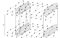
Figure 1. Informal illustration of Causal Graph Dynamics.

CGD were motivated by the countless situations featuring nearest-neighbours interactions with time-varying neighbourhood (e.g. agents exchange contacts, move around…). Many existing models (of complex systems, computer processes, biochemical agents, economical agents, social networks…) fall into this category, thereby generalizing CA for their specific sake (e.g. self-reproduction as [30], discrete general relativity à la Regge calculus [28], etc.). CGD are a theoretical framework, for these models. Some graph rewriting models, such as Amalgamated Graph Transformations [9] and Parallel Graph Transformations [13, 29], also work out rigorous ways of applying a local rewriting rule synchronously throughout a graph, albeit with a different, category-theory-based perspective, of which the latest and closest instance is [24].

In [7, 6] one of the authors studied CGD in the reversible regime. Specific examples of these were described in [17, 22]. From a theoretical Computer Science perspective, the point was to generalize RCA theory to arbitrary, bounded-degree, time-varying graphs. Indeed the two main results were the generalizations of the two above-mentioned fundamental properties of RCA.

From a mathematical perspective, questions related to the bijectivity of CA over certain classes of graphs (more specifically, whether pre-injectivity implies surjectivity for Cayley graphs generated by certain groups [8, 14, 15]) have received quite some attention. The present paper on the other hand provides a context in which to study “bijectivity of CA over time-varying graphs”. We answer the question: Is it the case that bijectivity necessarily rigidifies space (i.e. forces the conservation of each vertex)?

From a theoretical physics perspective, the question whether the reversibility of small scale physics (quantum mechanics, micro-mechanical), can be reconciled with the time-varying topology of large scale physics (relativity), is a major challenge. This paper provides a rigorous discrete, toy model where reversibility and time-varying topology coexist and interact—in a way which does allow for space expansion. In fact these results open the way for Quantum Causal Graph Dynamics [5] allowing for vertex creation/destruction—which could provide a rigorous basic formalism to use in Quantum Gravity [23, 16].

3. In a nutshell : Reversible Causal Graph Dynamics

The following provides an intuitive introduction to Reversible CGD. A thorough formalization was given in [2], and is reproduced in Appendix A [ArrighiIMRCGD].

Networks. Whether for CA over graphs [26], multi-agent modeling [11] or agent-based distributed algorithms [10], it is common to work with graphs whose nodes have numbered neighbours. Thus our ’graphs’ or networks are the usual, connected, undirected, possibly infinite, bounded-degree graphs, but with a few additional twists:

• The set $\pi$ of available ports to each vertex is finite.

• The vertices are connected through their ports: an edge is an unordered pair $\{u:a,v:b\}$, where $u,v$ are vertices and $a,b\in\pi$ are ports. Each port is used at most once: if both $\{u:a,v:b\}$ and $\{u:a,w:c\}$ are edges, then $v=w$ and $b=c$. As a consequence the degree of the graph is bounded by $|\pi|$.

• The vertices and edges can be given labels taken in finite sets $\Sigma$ and $\Delta$ respectively, so that they may carry an internal state.

• These labeling functions are partial, so that we may express our partial knowledge about part of a graph.

The set of all graphs (see Figure 2$(a)$) is denoted $\mathcal{G}_{\Sigma,\Delta,\pi}$.

Compactness. In order to both drop the irrelevant names of nodes and obtain a compact metric space of graphs, we need ’pointed graphs modulo’ instead:

• The graphs has a privileged pointed vertex playing the role of an origin.

• The pointed graphs are considered modulo isomorphism, so that only the relative position of the vertices can matter.

The set of all pointed graphs modulo (see Figure 2$(c)$) is denoted $\mathcal{X}_{\Sigma,\Delta,\pi}$.
If, instead, we drop the pointers but still take equivalence classes modulo isomorphism, we obtain just graphs modulo, aka ’anonymous graphs’. The set of all anonymous graphs (see Figure 2$(d)$) is denoted $\mathcal{\widetilde{X}}_{\Sigma,\Delta,\pi}$.

Figure 2. The different types of graphs. (a) A graph $G$. (b) A pointed graph $(G,1)$. (c) A pointed graph modulo $X$. (d) An anonymous graph $\widetilde{X}$.

Operations over graphs. Given a pointed graph modulo $X$, $X^{r}$ denotes the sub-disk of radius $r$ around the pointer. The pointer of $X$ can be moved along a path $u$, leading to $Y=X_{u}$. We use the notation $X_{u}^{r}$ for $(X_{u})^{r}$ i.e., first the pointer is moved along $u$, then the sub-disk of radius $r$ is taken.

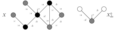
Figure 3. Operations over pointed graphs modulo. The pointer of $X$ is shifted along edge $ad$, yielding $X_{ad}$, and then the disk of radius $0$ around the pointer, yielding $X^{0}_{ad}$.

Causal Graph Dynamics. We will now recall their topological definition. It is important to provide a correspondence between the vertices of the input pointed graph modulo $X$, and those of its image $F(X)$, which is the role of $R_{X}$:

Definition 3.1 (Dynamics).

A dynamics $(F,R_{\bullet})$ is given by

• a function $F\colon{\cal X}_{\Sigma,\Delta,\pi}\to{\cal X}_{\Sigma,\Delta,\pi}$;

• a map $R_{\bullet}$, with $R_{\bullet}\colon X\mapsto R_{X}$ and $R_{X}:V(X)\to V(F(X))$.

Next, continuity is the topological way of expressing causality:

Definition 3.2 (Continuity).

A dynamics $(F,R_{\bullet})$ is said to be continuous if and only if for any $X$ and $m$, there exists $n$, such that

$$\bullet\ F(X)^{m}=F(X^{n})^{m}\qquad\bullet\ \textrm{dom}\,R_{X}^{m}\subseteq V(X^{n})\textrm{ and }R_{X}^{m}=R_{X^{n}}^{m}$$

where $R_{X}^{m}$ denotes the partial map obtained as the restriction of $R_{X}$ to the co-domain $F(X)^{m}$, using the natural inclusion of $F(X)^{m}$ into $F(X)$.

Notice that the second condition states the continuity of $R_{\bullet}$ itself. A key point is that by compactness, continuity entails uniform continuity, meaning that $n$ does not depend upon $X$—so that the above really expresses that information has a bounded speed of propagation of information.
We now express that the same causes lead to the same effects:

Definition 3.3 (Shift-invariance).

A dynamics $(F,R_{\bullet})$ is said to be shift-invariant if for every $X$, $u\in X$, and $v\in X_{u}$,

$$\bullet\ F(X_{u})=F(X)_{R_{X}(u)}\qquad\bullet\ R_{X}(u.v)=R_{X}(u).R_{X_{u}}(v)$$

Finally we demand that graphs do not expand in an unbounded manner:

Definition 3.4 (Boundedness).

A dynamics $(F,R_{\bullet})$ is said to be bounded if there exists a bound $b$ such that for any $X$ and any $w^{\prime}\in F(X)$, there exists $u^{\prime}\in\textrm{Im}(R_{X})$ and $v^{\prime}\in F(X)_{u^{\prime}}^{b}$ such that $w^{\prime}=u^{\prime}.v^{\prime}$.

Putting these conditions together yields the topological definition of CGD:

Definition 3.5 (Causal Graph Dynamics).

A CGD is a shift-invariant, continuous, bounded dynamics.

Reversibility. Invertibility is imposed in the most general and natural fashion.

Definition 3.6 (Invertible dynamics).

A dynamics $(F,R_{\bullet})$ is said to be invertible if $F$ is a bijection.

Unfortunately, this condition turns out to be very limiting. It is the following limitation that the present paper seeks to circumvent:

Theorem 3.7 (Invertible implies almost-vertex-preserving [7]).

Let $(F,R_{\bullet})$ be an invertible CGD. Then there exists a bound $p$, such that for any graph $X$, if $|V(X)|>p$ then $R_{X}$ is bijective.

On the face of it reversibility is stronger a stronger condition than invertibility:

Definition 3.8 (Reversible Causal Graph Dynamics).

A CGD $(F,R_{\bullet})$ is reversible if there exists $S_{\bullet}$ such that $(F^{-1},S_{\bullet})$ is a CGD.

Fortunately, invertibility gets you reversibility:

Theorem 3.9 (Invertible implies reversible [7]).

If $(F,R_{\bullet})$ is an invertible CGD, then $(F,R_{\bullet})$ is reversible.

As a simple example we provide an original, general scheme for propagating particles on an arbitrary network in a reversible manner:

Example 3.10 (General reversible advection).

Consider $\pi=\{a,b,\ldots\}$ a finite set of ports, and let $\Sigma={\cal P}(\pi)$ be the set of internal states, where: $\varnothing$ means ‘no particle is on that node’; $\{a\}$ means ‘one particle is set to propagate along port $a$’; $\{a,b\}$ means ‘one particle is set to propagate along port $a$ and another along port $b$’…. Let $s$ be a bijection over the set of ports, standing for the successor direction. Fig. 4$(a)$ specifies how individual particles propagate. Basically, when reaching its destination, the particle set to propagate along the successor of the port it came from. Missing edges behave like self-loops. Applying this to all particles synchronously specifies the ACGD.

4. The anonymous solution

Having a pointer is essential in order to express causality, but cumbersome when it comes to reversibility. Here is the direct way to get the best of both worlds.

Definition 4.1 (Anonymous Causal Graph Dynamics).

Consider $\widetilde{F}$ a function over $\mathcal{\widetilde{X}}_{\Sigma,\Delta,\pi}$. We say that $\widetilde{F}$ is an ACGD if and only if there exists $(F,R_{\bullet})$ a CGD such that $F$ over $\mathcal{X}_{\Sigma,\Delta,\pi}$ naturally induces $\tilde{F}$ over $\mathcal{\widetilde{X}}_{\Sigma,\Delta,\pi}$.

Invertibility, then, just means that $\widetilde{F}$ is bijective. Fortunately, this time the condition is not so limiting, and we are able to implement non-vertex-preserving dynamics, as can be seen from this slight generalization of the HM example:

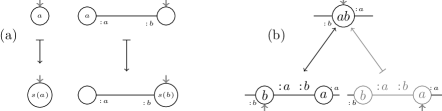
Figure 4. $(a)$ General reversible advection. $(b)$ The HM example’s collision step. The anonymous dynamics is in plain black, the underlying regular dynamics is in grey.

Example 4.2 (Anonymous HM).

. Consider the state space of Example 3.10 and alternate: 1. a step of advection as in Fig. 4$(a)$, 2. a step of collision, where the collision is the specific graph replacement provided in Fig. 4$(b)$. The composition of these two specifies the ACGD.

So, ACGD feature local vertex creation/destruction. Yet they are clearly less constructive than CGD, as $R_{\bullet}$ is no longer explicit. In spite of this lack of constructiveness, we still have

Theorem 4.3 (Anonymous invertible implies reversible).

If an ACGD in invertible, then the inverse function is an ACGD.

Proof outline. By Th. 7.1 the invertible ACGD $\widetilde{F}$ can be directly simulated by an invertible IMCGD, see next. By Th. 5.5 the inverse IMCGD is also an IMCGD. Dropping the invisible matter of this inverse provides the CGD that underlines $\widetilde{F}^{-1}$. $\square$

5. The Invisible Matter solution

Reversible CGD are vertex-preserving. Still, we could think of using them to simulate a non-vertex-preserving dynamics by distinguishing ‘visible’ and ‘invisible matter’, and making sure that every visible node is equipped with its own reservoir of ‘invisible’ nodes—in which it can tap. For this scheme to iterate, and for the infanted nodes to be able to create nodes themselves, it is convenient to shape the reservoirs as everywhere infinite binary trees.

Definition 5.1 (Invisible Matter Graphs).

Consider ${\cal X}={\cal X}_{\Sigma,\Delta,\pi}$, ${\cal T}={\cal X}_{\{m\},\emptyset,\{m,l,r\}}$ and ${\cal X}^{\prime}={\cal X}_{\Sigma\cup\{m\},\Delta,\pi\cup\{m,l,r\}}$, assuming that $\{m\}\cap\Sigma=\emptyset$ and $\{m,l,r\}\cap\pi=\emptyset$. Let $T\in{\cal T}$ be the infinite binary tree whose origin $\varepsilon$ has a copy of $T$ at vertex $lm$, and another at vertex $rm$. Every $X\in{\cal X}$ can be identified to an element of ${\cal X}^{\prime}$ obtained by attaching an instance of $T$ at each vertex through path $mm$. The hereby obtained graphs will be denoted ${\cal Y}$ and referred to as invisible matter graphs.

We will now consider those CGD over ${\cal X^{\prime}}$ that leave ${\cal Y}$ stable. In fact we want them trivial as soon as we dive deep enough into the invisible matter:

Definition 5.2 (Invisible-matter quiescence).

A dynamic $(F,R_{\bullet})$ over ${\cal Y}$ is said invisible matter quiescent if there exists a bound $b$ such that, for all $X_{{{{\bullet}}}s}$, and for all $t$ in $\{lm,rm\}^{*}$, we have $|s|\geq b\implies R_{X_{{{{\bullet}}}s}}(t)=t$.

Definition 5.3 (Invisible Matter Causal Graph Dynamics).

A CGD over ${\cal Y}$ is said to be an IMCGD if and only if it is vertex-preserving and invisible matter quiescent.

Fortunately, we are indeed able to encode non-vertex-preserving dynamics in the visible sector of an invertible IMCGD:

Figure 5. HM example’s collision step with pointers and invisible matter. Black vertices are ‘invisible’. The dotted lines show where to place the pointer in the image according to its position in the antecedent.

Example 5.4 (Invisible Matter HM).

Consider X as in Example 3.10 and extend it to Y. Alternate: 1. a step of advection as in Example 3.10 and 4$(a)$, 2. a step of collision, where the collision is the specific graph replacement provided in Fig. 5. The composition of these two specifies the invertible IMCGD.

Notice how the graph replacement of Fig. 4$(b)$—with the grey color taken into account—would fail to be invertible, due to the collapsing of two pointer positions into one.
Fortunately also, invertibility still implies reversibility:

Theorem 5.5 (Invertible implies reversible).

If $(F,R_{\bullet})$ is an invertible IMCGD, then $(F^{-1},R_{F^{-1}(\bullet)}^{-1})$ is an IMCGD.

Proof outline. Intuitively this property is inherited from that of CGD over ${\cal X}^{\prime}$. Th. 3.9, however, relies on the compactness of ${\cal X}^{\prime}$, and as matter of fact ${\cal Y}$ is not compact. Still it admits a compact closure $\overline{{\cal Y}}$, over which IMCGD have a natural, continuous extension, see Appendix B of [ArrighiIMRCGD]. $\Box$

6. The Name Algebra solution

So far we worked with (pointed) graphs modulo. But named graphs are often more convenient e.g. for implementation, and sometimes mandatory e.g. for studying the quantum case[5]. In this context, being able to locally create a node implies being able to locally make up a new name for it—just from the locally available ones. For instance if a dynamics $F$ splits a node $u$ into two, a natural choice is to call these $u.l$ and $u.r$. Now, apply a renaming $R$ that maps $u.l$ into $v$ and $u.r$ into $w$, and apply $F^{-1}$. This time the nodes $v$ and $w$ get merged into one; in order not to remain invertible a natural choice is to call the resultant node $(v\wedge w)$. Yet, if $R$ is chosen trivial, then the resultant node is $(u.l\wedge u.r)$, when $F^{-1}\circ F=Id$ demands that this to be $u$ instead. This suggests considering a name algebra where $u=(u.l\wedge u.r)$.

Definition 6.1 (Name Algebra).

Let ${\cal N}$ be a countable set (eg ${\cal N}=\mathbb{N}$). Consider the terms produced by the grammar $V::={\cal N}\,|\,V.\{l,r\}^{*}\,|\,V\wedge V$ together with the equivalence induced by the term rewrite systems

$$\bullet\quad(u\wedge v).l\longrightarrow u\qquad(u\wedge v).r\longrightarrow v\qquad(S)\qquad\textrm{and}\qquad\bullet\quad(u.l\wedge u.r)\longrightarrow u\qquad(M)$$

i.e. $u$ and $v$ are equivalent if and only if their normal forms $u\!\downarrow_{S\cup M}$ and $v\!\downarrow_{S\cup M}$ are equal.

Well-foundedness outline. The TRS was checked terminating and locally confluent using CiME, hence its confluence and the unicity of normal forms via Church-Rosser. $\Box$
This is the algebra of symbolic everywhere infinite binary trees. Indeed, each element $x$ of ${\cal N}$ can be thought of as a variable representing an infinite binary tree. The $.l$ (resp. $.r$) projection operation recovers the left (resp. right) subtree. The ‘join’ operation $\wedge$ puts a node on top of its left and right trees to form another—it is therefore not commutative nor associative. This infinitely splittable/mergeable tree structure is reminiscent of Section 5, later we shall prove that named graphs arise by abstracting away the invisible matter.
No graph can have two distinct nodes called the same. Nor should it be allowed to have a node called $x$ and two others called $x.r$ and $x.l$, because the latter may merge and collide with the former.

Definition 6.2 (Intersectant).

Consider $G,G^{\prime}$ in ${\cal W}$. Two vertices $v$ in $G$ and $v^{\prime}$ in $G^{\prime}$ are said to be intersectant if and only if there exists $t,t^{\prime}$ in $\{l,r\}^{*}$ such that $v.t=v^{\prime}.t^{\prime}$. We then write $\iota(v,v^{\prime})$. We also write $\iota(v,V(G^{\prime}))$ if and only if there exists $v^{\prime}$ in $G^{\prime}$ such that $\iota(v,v^{\prime})$.

Definition 6.3 (Well-named graphs.).

We say that a graph $G$ is well-named if and only if for all $v,v^{\prime}$ in $G$ and $t,t^{\prime}$ in $\{l,r\}^{*}$ then $v.t=v^{\prime}.t^{\prime}$ implies $v=v^{\prime}$ and $t=t^{\prime}$. We denote by ${\cal W}$ the subset of well-named graphs.

We now have all the ingredients to define Named Causal Graph Dynamics.

Definition 6.4 (Continuity).

A function $\overline{F}$ over ${\cal W}$ is said to be continuous if and only if for any $G$ and any $n\geq 0$, there exists $m\geq 0$, such that for all $v^{\prime}$, for all $\iota(v,v^{\prime})$, $\overline{F}(G)^{n}_{v^{\prime}}=\overline{F}(G^{m}_{v})^{n}_{v^{\prime}}$

Definition 6.5 (Renaming).

Consider $R$ an injective function from ${\cal N}$ to $V$ such that for any $x,y\in{\cal N}$, $R(x)$ and $R(y)$ are not intersectant. The natural extension of $R$ to the whole of $V$, according to

$$R(u.l)=R(u).l\qquad R(u.r)=R(u).r\qquad R(u\wedge v)=R(u)\wedge R(v)$$

is referred to as a renaming.

Definition 6.6 (Shift-invariance).

A function $\overline{F}$ over ${\cal W}$ is said to be shift-invariant if and only if for any $G\in{\cal W}$ and any renaming $R$, $F(RG)=RF(G)$.

Our dynamics may split and merge names, but not drop them:

Definition 6.7 (Name-preservation).

Consider $\overline{F}$ a function over ${\cal W}$. The function $\overline{F}$ is said to be name-preserving if and only if for all $u$ in $V$ and $G$ in ${\cal W}$ we have that $\iota(u,V(G))$ is equivalent to $\iota(u,V(\overline{F}(G)))$.

Definition 6.8 (Named Causal Graph Dynamics).

A function $\overline{F}$ over ${\cal W}$ is said to be a Named Causal Graph Dynamics (NCGD) if and only if is shift-invariant, continuous, and name-preserving.

Fortunately, invertible NCGD do allow for local creation/destruction of vertices:

Figure 6. The HM example’s collision step for Named CGD.

Example 6.9 (Named HM example).

Consider W with ports and labels as in Example 3.10. Alternate: 1. a step of advection as in Example 3.10 and 4$(a)$, 2. a step of collision, where the collision is the specific graph replacement provided in Fig. 6 That the latter is an involution follows from the three equalities holding in $V$.

Fortunately also, invertibility still implies reversibility.

Theorem 6.10 (Named invertible implies reversible).

If an NCGD in invertible, then the inverse function is an NCGD.

Proof outline. By Th. 7.3 the invertible NCGD $\overline{F}$ can be directly simulated by an invertible IMCGD $(F,R_{\bullet})$, whose pointer mimics the behaviour of atomic names. Its inverse $(F^{-1},R_{F^{-1}(\bullet)}^{-1})$ thus captures the full behaviour of $\overline{F}^{-1}$ over graphs including vertex names. By Th. 5.5 $(F^{-1},R_{F^{-1}(\bullet)}^{-1})$ is continuous, and thus so is $\overline{F}^{-1}$. $\square$

7. Robustness

Previous works gave three negative results about the ability to locally create/destroy nodes in a reversible setting. But we just described three relaxed settings in which this is possible. The question is thus formalism-dependent. How sensitive is it to changes in formalism, exactly? We show that the three solutions directly simulate each other. They are but three presentations, in different levels of details, of a single robust solution.

In what follows $\alpha$ is the natural, surjective map from ${\cal Y}$ to ${\cal\widetilde{X}}$, which (informally) : 1. Drops the pointer and 2. Cuts out the invisible matter. Whatever an ACGD does to a $\alpha(Y)$, an IMCGD can do to $Y$—moreover the notions of invertibility match:

Theorem 7.1 (IMCGD simulate ACGD).

Consider $\widetilde{F}$ an ACGD. Then there exists $(F,R_{\bullet})$ an IMCGD such that for all but a finite number of graphs $Y$ in ${\cal Y}$, $\widetilde{F}(\alpha(Y))=\alpha(F(Y))$. Moreover if $\widetilde{F}$ is invertible, then this $(F,R_{\bullet})$ is invertible.

Proof outline. Any ACGD $\widetilde{F}$ has an underlying CGD $(F,R_{\bullet})$. We show it can be extended to invisible matter, an then mended to make $R_{\bullet}$ bijective, thereby obtaining an IMCGD. The precise way this is mended relies on the fact vertex creation/destruction cannot happen without the presence of a local asymmetry—except in a finite number of cases. Next, bijectivity upon anonymous graphs induces bijectivity upon pointed graphs modulo. $\square$
Similarly, whatever an IMCGD does to a $Y$, a ACGD can do to $\alpha(Y)$:

Theorem 7.2 (ACGD simulate IMCGD).

Consider $(F,R_{\bullet})$ an IMCGD. Then there exists an ACGD such that $\widetilde{F}\circ\alpha=\alpha\circ F$. Moreover if $(F,R_{\bullet})$ is invertible, then this $\widetilde{F}$ is invertible.

Proof outline. The ACGD is obtained by dropping the pointer and the invisible matter. $\square$
In what follows, if $G$ is a graph in $\cal W$, then $G^{\prime}$ is the graph obtained from $G$ by attaching invisible–matter trees to each vertex, and naming the attached vertices in $V(G).\{l,r\}^{*}$ according to Fig. 7. $\square$

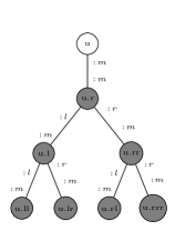
Figure 7. Conventions for naming the invisible–matter.

Theorem 7.3 (IMCGD simulate NCGD).

Consider $\overline{F}$ an NCGD. There exists $\overline{R}_{\bullet}$ such that for all $G$, $\overline{R}_{G}$ is a bijection from $V(G).\{l,r\}^{*}$ to $V(F(G)).\{l,r\}^{*}$. This induces an IMCGD $(F,R_{\bullet})$ via

• $F(\widetilde{(G^{\prime},u.t)})=\widetilde{(\overline{F}(G)^{\prime},\overline{R}_{G}(u.t))}$.

• $R_{\widetilde{(G^{\prime},u.t)}}(p)$ is the path between $\overline{R}_{G}(u.t)$ and $\overline{R}_{G}(v.s)$ in $\overline{F}(G)^{\prime}$, where $v.s$ is obtained by following path $p$ from $u.t$ in $G^{\prime}$.

Moreover if $\overline{F}$ is invertible, then this $(F,R_{\bullet})$ is invertible.

Proof outline. The names $V(\overline{F}(G))$ can be understood as keeping track of the splits and mergers that have happened through the application of $\overline{F}$ to $G$, as in Fig. 6. $\overline{R}_{\bullet}$ uses this to build a bijection from $V(G^{\prime})$ to $V(\overline{F}(G)^{\prime})$, following conventions as in Fig. 5. $\square$

Theorem 7.4 (NCGD simulate IMCGD).

Consider $(F,R_{\bullet})$ an IMCGD. Then there exists $\overline{F}$ an NCGD such that for all graphs $Y=\widetilde{(G,u)}$ in $\cal Y$, $F(Y)=\widetilde{(\overline{F}(G),u)}$. Moreover $F$ is invertible if and only if $\overline{F}$ is invertible.

Proof outline. Each vertex of $Y$ can be named so that the resulting graph $G$ is well-named. Then $R_{\bullet}$ is used to construct the behaviour of $\overline{F}$ over names of vertices. As $(F,R_{\bullet})$ does not merge nor split vertices, $F$ preserves the name of each vertex. $\square$

Thus, NCGD are more detailed than IMCGD, which are more detailed than ACGD. But, if one is thought of as retaining just the interesting part of the other, it does just what the other would do to this interesting part—and no more.

8. Conclusion

Summary of contributions. We have raised the question whether parallel reversible computation allows the local creation/destruction of nodes. Different negative answers had been given in [1, 4, 7] which inspired us with three relaxed settings: Causal Graph Dynamics over fully-anonymized graphs (ACGD); over pointer graphs modulo with invisible matter reservoirs (IMCGD); and finally CGD over graphs whose vertex names are in the algebra of ‘everywhere infinite binary trees’ (NCGD). For each of these formalism, we proved non-vertex-preservingness by implementing the Hasslacher-Meyer example [17]—see Examples 4.2,5.4, 6.9. We also proved that we still had the classic Cellular Automata (CA) result that invertibility (i.e. mere bijectivity of the dynamics) implies reversibility (i.e. the inverse is itself a CGD)—via compactness—see Theorems 4.3,5.5, 6.10. The answer to the question of reversibility versus local creation/destruction is thus formalism-dependent to some extent. We proceeded to examine the extent in which this is the case, and were able to show that (Reversible) ACGD, IMCGD and NCGD directly simulate each other—see Theorems 7.1, 7.2, 7.3, 7.4. They are but three presentations, in different levels of details, of a single robust setting in which reversibility and local creation/destruction are reconciled.

Perspectives. Just like Reversible CA were precursors to Quantum CA [27, 3], Reversible CGD have paved the way for Quantum CGD [5]. Toy models where time-varying topologies are reconciled with quantum theory, are of central interest to the foundations of theoretical physics [23, 16]—as it struggles to have general relativity and quantum mechanics coexist and interact. The ‘models of computation approach’ brings the clarity and rigor of theoretical CS to the table, whereas the ‘natural and quantum computing approach’ provides promising new abstractions based upon ‘information’ rather than ‘matter’. Quantum CGD [5], however, lacked the ability to locally create/destroy nodes—which is necessary in order to model physically relevant scenarios. Our next step will be to apply the lessons learned, to fix this.

Appendix A Formalism

This appendix provides formal definitions of the kinds of graphs we are using, together with the operations we perform upon them. None of this is specific to the reversible case; it can all be found in [2] and is reproduced here only for convenience.

A.1. Graphs

Let $\pi$ be a finite set, $\Pi=\pi^{2}$, and $V$ some universe of names.

Definition A.1 (Graph non-modulo).

A graph non-modulo $G$ is given by

• An at most countable subset $V(G)$ of $V$, whose elements are called vertices.

• A finite set $\pi$, whose elements are called ports.

• A set $E(G)$ of non-intersecting two element subsets of $V(G):\pi$, whose elements are called edges. In other words an edge $e$ is of the form $\{u:a,v:b\}$, and $\forall e,e^{\prime}\in E(G),e\cap e^{\prime}\neq\emptyset\Rightarrow e=e^{\prime}$.

• A partial function $\sigma$ from $V(G)$ to a finite set $\Sigma$;

• A partial function $\delta$ from $V(G)$ to a finite set $\Delta$;

The graph is assumed to be connected: for any two $u,v\in V(G)$, there exists $v_{0},\ldots,v_{n}\in V(G)$, $a_{0},b_{0}\ldots,a_{n-1},b_{n-1}\in\pi$ such that for all $i\in\{0\ldots n-1\}$, one has $\{v_{i}:a_{i},v_{i+1}:b_{i}\}\in E(G)$ with $v_{0}=u$ and $v_{n}=v$.
The set of graphs with states in $\Sigma,\Delta$ and ports $\pi$ is written ${\cal G}_{\Sigma,\Delta,\pi}$.

We single out a vertex as the origin:

Definition A.2 (Pointed graph non-modulo).

A pointed graph is a pair $(G,p)$ with $p\in G$. The set of pointed graphs with states in $\Sigma,\Delta$ and ports $\pi$ is written ${\cal P}_{\Sigma,\Delta,\pi}$.

Here is when graph differ only up to names of vertices:

Definition A.3 (Isomorphism).

An isomorphism $R$ is a function from ${\cal G}_{\pi}$ to ${\cal G}_{\pi}$ which is specified by a bijection $R(.)$ from $V$ to $V$. The image of a graph $G$ under the isomorphism $R$ is a graph $RG$ whose set of vertices is $R(V(G))$, and whose set of edges is $\{\{R(u):a,R(v):b\}\;|\;\{u:a,v:b\}\in E(G)\}$. Similarly, the image of a pointed graph $P=(G,p)$ is the pointed graph $RP=(RG,R(p))$. When $P$ and $Q$ are isomorphic we write $P\approx Q$, defining an equivalence relation on the set of pointed graphs. The definition extends to pointed labeled graphs.

(Pointed graph isomorphism rename the pointer in the same way as it renames the vertex upon which it points; which effectively means that the pointer does not move.)

Definition A.4 (Pointed graphs modulo).

Let $P$ be a pointed (labeled) graph $(G,p)$. The pointed graph modulo $X(P)$ is the equivalence class of $P$ with respect to the equivalence relation $\approx$. The set of pointed graphs modulo with ports $\pi$ is written ${\cal X}_{\pi}$. The set of labeled pointed Graphs modulo with states $\Sigma,\Delta$ and ports $\pi$ is written ${\cal X}_{\Sigma,\Delta,\pi}$.

A.2. Paths and vertices

Vertices of pointed graphs modulo isomorphism can be designated by a sequence of ports in $\Pi^{*}$ that leads, from the origin, to this vertex.

Definition A.5 (Path).

Given a pointed graph modulo $X$, we say that $\alpha\in\Pi^{*}$ is a path of $X$ if and only if there is a finite sequence $\alpha=(a_{i}b_{i})_{i\in\{0,...,n-1\}}$ of ports such that, starting from the pointer, it is possible to travel in the graph according to this sequence. More formally, $\alpha$ is a path if and only if there exists $(G,p)\in X$ and there also exists $v_{0},\ldots,v_{n}\in V(G)$ such that for all $i\in\{0\ldots n-1\}$, one has $\{v_{i}:a_{i},v_{i+1}:b_{i}\}\in E(G)$, with $v_{0}=p$ and $\alpha_{i}=a_{i}b_{i}$. Notice that the existence of a path does not depend on the choice of $(G,p)\in X$. The set of paths of $X$ is denoted by $V(X)$.

Paths can be seen as words on the alphabet $\Pi$ and thus come with a natural operation ‘.’ of concatenation, a unit $\varepsilon$ denoting the empty path, and a notion of inverse path $\overline{\alpha}$ which stands for the path $\alpha$ read backwards. Two paths are equivalent if they lead to same vertex:

Definition A.6 (Equivalence of paths).

Given a pointed graph modulo $X$, we define the equivalence of paths relation $\equiv_{X}$ on $V(X)$ such that for all paths $\alpha,\alpha^{\prime}\in V(X)$, $\alpha\equiv_{X}\alpha^{\prime}$ if and only if, starting from the pointer, $\alpha$ and $\alpha^{\prime}$ lead to the same vertex of $X$. More formally, $\alpha\equiv_{X}\alpha^{\prime}$ if and only if there exists $(G,p)\in X$ and $v_{1},\ldots,v_{n},v^{\prime}_{1},\ldots,v^{\prime}_{n^{\prime}}\in V(G)$ such that for all $i\in\{0\ldots n-1\}$, $i^{\prime}\in\{0\ldots n^{\prime}-1\}$, one has $\{v_{i}:a_{i},v_{i+1}:b_{i}\}\in E(G)$, $\{v^{\prime}_{i^{\prime}}:a^{\prime}_{i^{\prime}},v^{\prime}_{i^{\prime}+1}:b^{\prime}_{i^{\prime}}\}\in E(G)$, with $v_{0}=p$, $v^{\prime}_{0}=p$, $\alpha=(a_{i}b_{i})_{i\in\{0,...,n-1\}}$, $\alpha^{\prime}=(a^{\prime}_{i^{\prime}}b^{\prime}_{i^{\prime}})_{i\in\{0,...,n^{\prime}-1\}}$ and $v_{n}=v_{n^{\prime}}$. We write $\hat{\alpha}$ for the equivalence class of $\alpha$ with respect to $\equiv_{X}$.

It is useful to undo the modulo, i.e. to obtain a canonical instance $(G(X),\varepsilon)$ of the equivalence class $X$.

Definition A.7 (Associated graph).

Let $X$ be a pointed graph modulo. Let $G(X)$ be the graph such that:

• The set of vertices $V(G(X))$ is the set of equivalence classes of $V(X)$;

• The edge $\{\hat{\alpha}:a,\hat{\beta}:b\}$ is in $E(G(X))$ if and only if $\alpha.ab\in V(X)$ and $\alpha.ab\equiv_{X}\beta$, for all $\alpha\in\hat{\alpha}$ and $\beta\in\hat{\beta}$.

We define the associated graph to be $G(X)$.

Notations. The following are three presentations of the same mathematical object:

• a graph modulo $X$,

• its associated graph $G(X)$

• the algebraic structure $\langle V(X),\equiv_{X}\rangle$

Each vertex of this mathematical object can thus be designated by

• $\hat{\alpha}$ an equivalence class of $V(X)$, i.e. the set of all paths leading to this vertex starting from $\hat{\varepsilon}$,

• or more directly by $\alpha$ an element of an equivalence class $\hat{\alpha}$ of $X$, i.e. a particular path leading to this vertex starting from $\varepsilon$.

These two remarks lead to the following mathematical conventions, which we adopt for convenience:

• $\hat{\alpha}$ and $\alpha$ are no longer distinguished unless otherwise specified. The latter notation is given the meaning of the former. We speak of a “vertex” $\alpha$ in $V(X)$ (or simply $\alpha\in X$).

• It follows that ‘$\equiv_{X}$’ and ‘$=$’ are no longer distinguished unless otherwise specified. The latter notation is given the meaning of the former. I.e. we speak of “equality of vertices” $\alpha=\beta$ (when strictly speaking we just have $\hat{\alpha}=\hat{\beta}$).

A.3. Operations over pointed Graphs modulo

Sub-disks. For a pointed graph $(G,p)$ non-modulo:

• the neighbours of radius $r$ are just those vertices which can be reached in $r$ steps starting from the pointer $p$;

• the disk of radius $r$, written $G^{r}_{p}$, is the subgraph induced by the neighbours of radius $r+1$, with labellings restricted to the neighbours of radius $r$ and the edges between them, and pointed at $p$.

For a graph modulo, on the other hand, the analogous operation is:

Definition A.8 (Disk).

Let $X\in{\cal X}_{\Sigma,\Delta,\pi}$ be a pointed graph modulo and $G$ its associated graph. Let $X^{r}$ be $X(G^{r}_{\varepsilon})$. The graph modulo $X^{r}\in{\cal X}_{\Sigma,\pi}$ is referred to as the disk of radius $r$ of $X$. The set of disks of radius $r$ with states $\Sigma,\Delta$ and ports $\pi$ is written ${\cal X}^{r}_{\Sigma,\Delta,\pi}$.

Definition A.9 (Size).

Let $X\in{\cal X}_{\Sigma,\Delta,\pi}$ be a pointed graph modulo. We say that a vertex $u\in X$ has size less or equal to $r+1$, and write $|u|\leq r+1$, if and only if $u\in X^{r}$.

Shifts just move the pointer vertex:

Definition A.10 (Shift).

Let $X\in{\cal X}_{\Sigma,\Delta,\pi}$ be a pointed graph modulo and $G$ its associated graph. Consider $u\in X$ or $X^{r}$ for some $r$, and consider the pointed graph $(G,u)$, which is the same as $(G,\varepsilon)$ but with a different pointer. Let $X_{u}$ be $X(G,u)$. The pointed graph modulo $X_{u}$ is referred to as $X$ shifted by $u$.

Appendix B IMCGD : compactness & reversibility

Notations. In the rest of the paper, $X$ ranges over arbitrary elements of ${\cal X}$ and their natural identification in ${\cal Y}$, as given by Definition 5.1. Let $s$ be a word in $\{lm,rm\}^{*}$, we use $X_{{{{\bullet}}}s}$ as a shorthand notation for $X_{mms}$, i.e. the graph $X$ but pointed at $s$ within the nearest attached tree. Let $w$ be a word, then $[w]$ means either $w$ or the empty word $\varepsilon$.

B.1. Compactness

The main result of this subsection is that, although ${\cal Y}$ is not a compact subset of ${\cal X}^{\prime}$ by itself, IMCGD can be extended continuously over the compact closure of ${\cal Y}$ in ${\cal X}^{\prime}$.
Indeed ${\cal Y}$ is not a compact subset of ${\cal X}^{\prime}$, for instance the sequence $(X_{{{{\bullet}}}(lm)^{r}})_{r\in\mathbb{N}}$, pointing ever further into the invisible matter, has no convergent subsequence in ${\cal Y}$ but has one in $\mathcal{X}^{\prime}$.

Definition B.1 (Closure).

The compact closure of ${\cal Y}$ in ${\cal X}^{\prime}$, denoted $\overline{{\cal Y}}$, is the subset of elements $Y^{\prime}$ of ${\cal X}^{\prime}$ such that, for all $r$, there exists a $Y(r)$ in ${\cal Y}$ satisfying $Y(r)^{r}=Y^{\prime r}$.

Lemma B.2 (Visible starting paths).

Consider $Y^{\prime}$ in $\overline{{\cal Y}}$ with $\varepsilon$ visible, and $v$ in $Y^{\prime}$. Then $v$ can be decomposed as $u[{{{\bullet}}}t]$, with $u$ in $\Pi^{*}$, and $t$ in $\{lm,rm\}^{*}$. When $[{{{\bullet}}}t]$ is non-empty, $v$ is invisible. Moreover, for any $s,t$ in $\{lm,rm\}^{*}$, we have that ${{{\bullet}}}s,{{{\bullet}}}t$ are in $Y^{\prime}$, and ${{{\bullet}}}s\equiv_{Y^{\prime}}{{{\bullet}}}t$ if and only if $s=t$.

Proof B.3.

First consider $Y\in{\cal Y}$ with $\varepsilon$ visible. Clearly ${{{\bullet}}}s$ is in $Y$ and is the minimal path to ${{{\bullet}}}s$. Clearly also, $v$ can be minimally decomposed into $u[{{{\bullet}}}t]$ with $t$ in $\{lm,rm\}^{*}$, and when $t$ is non-empty, $v$ is invisible.
The same holds in the closure. Indeed consider $Y^{\prime}$ in $\overline{{\cal Y}}$ with $\varepsilon$ visible. Let $n=\max(|v|,|s|+1,|t|)$ and pick $Y$ in ${\cal Y}$ such that $Y^{\prime n}=Y^{n}$. By definition of $|v|$ we have that $p$ is a shortest path from $\varepsilon$ to $v$ in $Y$ if and only if it is one in $Y^{\prime}$. Therefore the form of the decomposition of $v$, and its invisibility when $t$ is not empty, carry through to $Y^{\prime}$. So does the existence of ${{{\bullet}}}s$. Finally, we have that ${{{\bullet}}}s\equiv_{Y^{\prime}}{{{\bullet}}}t$ implies ${{{\bullet}}}s\equiv_{Y}{{{\bullet}}}t$, which implies $s=t$, due to the tree structure of the invisible matter in $Y$.

Lemma B.4 (Invisible starting paths).

Consider $Y^{\prime}$ in $\overline{{\cal Y}}$ with $\varepsilon$ invisible, and $v$ in $Y^{\prime}$. Then $v$ can be decomposed as $\overline{s}{{{\bullet}}}u$, in which case $v$ is visible, or as $\overline{s}[{{{\bullet}}}u{{{\bullet}}}]t$, in which case $v$ is invisible—with $u$ in $\Pi^{*}$, and $s,t$ in $\{lm,rm\}^{*}$. Moreover, any $s,t$ in $\{lm,rm\}^{*}$, are also in $Y^{\prime}$, and we have that $s\equiv_{Y^{\prime}}t$ if and only if $s=t$.

Proof B.5.

Same proof scheme as in Lemma B.2.

Proposition B.6 (Closure of visible).

Consider $Y^{\prime}$ in $\overline{{\cal Y}}$ with $\varepsilon$ visible. Then $Y^{\prime}$ is in ${\cal Y}$.

Proof B.7.

Consider $v$ visible in $Y^{\prime}$. By the first part of Lemma B.2 the shortest path from $\varepsilon$ to $v$ is of the form $u{{{\bullet}}}t$ with $u$ in $\Pi^{*}$ and $t$ in $\{lm,rm\}^{*}$. But this $t$ needs be the empty word, otherwise $v$ would be invisible. Therefore visible nodes form a $\Pi^{*}$-connected component, call it $X$. By the second part of Lemma B.2 each vertex of $X$ has, in $Y^{\prime}$, an invisible matter tree attached to it—and no other invisible matter due again to the first part of Lemma B.2. Finally, there is no other invisible matter in $Y^{\prime}$ altogether, because $Y^{\prime}$ is connected.

Lemma B.8 (Finite invisible root).

Consider $Y^{\prime}$ in $\overline{{\cal Y}}$. If $Y^{\prime}$ has no visible matter, then, for all $n$, there exists a unique word $u_{n}$ in $\{lm,rm\}^{n}$ such that $Y^{n}=T_{u_{n}}^{n}$. As a consequence, $\overline{u}_{n}$ is the unique word in $\{ml,mr\}^{n}$ such that $\overline{u}_{n}$ is in $Y^{\prime}$. Moreover, if $p\leq n$, then $u_{p}$ is a suffix of $u_{n}$.

Proof B.9.

Consider $Y^{\prime}$ in $\overline{{\cal Y}}$. Pick $Y$ in ${\cal Y}$ such that $Y^{n}=Y^{\prime n}$. Since $Y^{\prime}$ has no visible vertex, $Y^{\prime}=Y_{{{{\bullet}}}s}$ with $|s|>n$, and we can take $u$ to be the suffix of length $n$ of $s$, and $t$ the complementary prefix, such that $s=tu$. $Y^{\prime n}$ is included in the invisible matter tree rooted in $Y_{{{{\bullet}}}t}$, hence $Y^{n}=Y^{\prime n}=(Y_{{{{\bullet}}}t})_{u}^{n}=T_{u}^{n}$.
For uniqueness, notice that for any two words $u,v$ of length $n$, $T_{u}^{n}=T_{v}^{n}$ implies $u=v$.
Since $\overline{u}_{n}$ is the only word of length $n$ in $\{ml,mr\}^{n}$ to represent a valid path of $Y^{\prime}$, its prefix of length $p$ is the only word of length $p$ in $\{ml,mr\}^{p}$ to represent a valid path of $Y^{\prime}$, which we know is $\overline{u}_{p}$.

Proposition B.10 (Closure of invisible).

$Y^{\prime}$ is in $\overline{{\cal Y}}$ and has no visible matter if and only if there exists $(u_{n})$ a sequence of path in $\{lm,rm\}^{n}$ such that $u_{n}$ suffix of $u_{n+1}$, $Y^{\prime n}=T_{u_{n}}^{n}$, and

$$Y^{\prime}=\bigcup\limits_{n=1}^{\infty}\nearrow T_{u_{n}}$$

i.e. $Y^{\prime}$ is the non-decreasing union of the $(T_{u_{n}})$.

Proof B.11.

First notice that $T_{v}$ is a sub-graph of $T_{uv}$. Indeed, by definition of $T$, the vertex $u$ in $T$ is the root of a copy of $T$, thus $T$ is a subgraph of $T_{u}$. Shifting this statement by $v$, $T_{v}$ is a sub-graph of $T_{uv}$. Thus it makes sense to speak about their non-decreasing union.
Next, for any $Y$, $Y=\bigcup\limits_{n=1}^{\infty}\nearrow Y^{n}$. So if $Y^{\prime}$ is a graph of $\overline{{\cal Y}}$ with no point in the visible matter, then

$$Y^{\prime}=\bigcup\limits_{n=1}^{\infty}\nearrow Y^{\prime n}=\bigcup\limits_{n=1}^{\infty}\nearrow T_{u_{n}}^{n}.$$

Reciprocally, any such non-decreasing union is equal to $\lim_{n}(X_{{{{\bullet}}}u_{n}})$, for any graph $X$ of ${\cal X}$ seen as an element of ${\cal Y}$, thus it belongs to ${\cal\overline{Y}}$.

Definition B.12.

Let $Y^{\prime}$ be a graph in $\overline{{\cal Y}}$ with no point in the visible matter and let $(u_{n})$ be the sequence of $\{lm,rm\}^{*}$ such that $Y^{n}=T_{u_{n}}^{n}$ and $u_{n}$ suffix of $u_{n+1}$. $Y$ being totally determined by the sequence $u$, we can write $Y=T_{u}$. The sequence $u$, growing for the suffix relation, can be identified with an infinite word of $\{lm,rm\}^{-\mathbb{N}}$, id est an infinite word with an end but no beginning.

Based on the previous results we have

Theorem B.13.

$$\overline{\cal Y}={\cal Y}\cup\{T_{u}:u\in\{lm,rm\}^{-\mathbb{N}}\}$$

Now that we know what the closure of ${\cal Y}$ looks like, we can try to extend IMCGD to it.

Proposition B.14.

Consider $(F,R_{\bullet})$ a continuous and shift-invariant dynamics over ${\cal Y}$. We have that $(F,R_{\bullet})$ is invisible matter quiescent if and only if $(F,R_{\bullet})$ can be continuously extended to ${\cal\overline{Y}}$ by letting $F(T_{u})=T_{u}$ and $R_{T_{u}}=Id$ for any $u$ in $\{l,r\}^{-\mathbb{N}}$.

Proof B.15.

Notice how, for all $Y$ and $u_{k+1}\in\{lm,rm\}^{k+1}\in Y$, we have that $Y_{u_{k+1}}^{k}=T_{u}^{k}$.
$[\Rightarrow]$. Let $(F,R_{\bullet})$ be a continuous, shift-invariant and invisible matter quiescent dynamics. Take $u$ a left-infinite word in $\{lm,rm\}^{-\mathbb{N}}$. Continuity of $F$ over ${\cal Y}$ states that for all $m$ there is an $n\geq m$ such that $F(Y)^{m}=F(Y^{n})^{m}$. By invisible matter quiescence there is a $b$ such that for all $X,p\in\{lm,rm\}^{b},v\in\{lm,rm\}^{*}$, $R_{X}({{{\bullet}}}pv)=R_{X}({{{\bullet}}}p)R_{X_{{{{\bullet}}}p}}(v)=R_{X}({{{\bullet}}}p)v$. Combining these, $F(T_{u}^{n})^{m}=F(X_{{{{\bullet}}}u_{b+n+1}}^{n})^{m}=F(X_{{{{\bullet}}}u_{b+n+1}})^{m}=F(X)_{R_{X}({{{{\bullet}}}u_{b}})u_{n+1}}^{m}=T_{u}^{m}$. Hence, if we extend $F$ to ${\cal\overline{Y}}$ by $F(T_{u})=T_{u}$, we get $F(T_{u})^{m}=F(T_{u}^{n})^{m}$, and so $F$ remains continuous. Similarly, continuity of $R_{\bullet}$ over ${\cal Y}$ states that for all $m$ there is an $n\geq m$ such that $R_{X}^{m}=R_{X^{n}}^{m}$. Again combining it with invisible matter quiescence, $R_{T_{u}^{n}}^{m}=R_{X_{{{{\bullet}}}u_{b+n+1}}^{n}}^{m}=Id$. Hence, if we extend $R$ to ${\cal\overline{Y}}$ by $R_{T_{u}}=Id$, we get $R_{T_{u}}^{m}=R_{T_{u}^{n}}^{m}$, and so $F$ remains continuous.
We can thus continuously extend $(F,R_{\bullet})$ by setting $F(T_{u})=T_{u}$ and $R_{T_{u}}=Id$.
$[\Leftarrow]$. Reciprocally, no longer assume invisible matter quiescence, and suppose instead that $(F,R_{\bullet})$, when extended by $F(T_{u})=T_{u}$ and $R_{T_{u}}=Id$, is continuous over $\overline{{\cal Y}}$. Since $\overline{{\cal Y}}$ is compact, $(F,R_{\bullet})$ is uniformly continuous (by the Heine–Cantor theorem). Take $c$ such that for all $Y$, $a$ in $Y$, and $|a|$=1, we have $|R_{Y}(a)|\leq c$. Such a $c$ exists by Lemma 3 of [2]. Take $b$ such that, for all $Y$, we have

$$\bullet\ F(Y)^{c}=F(Y^{b})^{c}\quad\bullet\ \textrm{dom}\,{R_{Y}}^{c}\subseteq V(Y^{b})\quad\bullet\ {R_{Y}}^{c}={R_{Y^{b}}}^{c}$$

We prove, by recurrence, that $b+1$ is the bound for invisible matter quiescence. Indeed, our recurrence hypothesis is that for all $p$ in $\{lm,rm\}^{b+1}$ and $w$ in $\{lm,rm\}^{n}$, we have $R_{X_{{{{\bullet}}}p}}(w)=w$. The hypothesis holds for $n=0$, because a consequence of shift-invariance is that $R_{Y}(\varepsilon)=\varepsilon$ for any $Y$. Suppose it holds for some $n$. Take $a$ in $\{lm,rm\}$. We have $R_{X_{{{{\bullet}}}p}}(wa)=R_{X_{{{{\bullet}}}p}}(w)R_{X_{{{{\bullet}}}pw}}(a)$. Since $|p|=b+1$ and, we have $X_{{{{\bullet}}}pw}^{b}=T_{upw}^{b}$ for any left-infinite $u$ in $\{lm,rm\}^{-\mathbb{N}}$. By the choice of $c$ and $b$, $R_{X_{{{{\bullet}}}pw}}(a)=R_{X_{{{{\bullet}}}pw}}^{c}(a)=R_{X_{{{{\bullet}}}pw}^{b}}^{c}(a)=R_{T_{upw}^{b}}^{c}(a)=R_{T_{upw}}^{c}(a)=Id^{c}(a)=a$. Putting things together, we have $R_{X_{{{{\bullet}}}p}}(wa)=wa$.

Theorem B.16.

An IMCGD can be extended into a vertex-preserving invisible matter quiescent CGD over $\overline{\cal Y}$.

Proof B.17.

Consider $(F,R_{\bullet})$ an IMCGD. Extend it to $\overline{\cal Y}$ by setting $F(T_{u})=T_{u}$ and $R_{T_{u}}=Id$. By Proposition B.14 the extension is still continuous. It is still vertex-preserving since $R_{T_{u}}$ is bijective. Therefore it is still bounded. It is still shift-invariant since $R_{T_{u}}(vw)=R_{T_{u}}(v)R_{T_{uv}}(w)=vw$.

Corollary B.18.

An IMCGD $(F,R_{\bullet})$ is uniformly continuous. I.e. for all $m$, there exists $n$, such that for any $X$,

$$\bullet\ F(X)^{m}=F(X^{n})^{m}\qquad\bullet\ \textrm{dom}\,R_{X}^{m}\subseteq V(X^{n})\textrm{ and }R_{X}^{m}=R_{X^{n}}^{m}$$

where $R_{X}^{m}$ denotes the partial map obtained as the restriction of $R_{X}$ to the co-domain $F(X)^{m}$, using the natural inclusion of $F(X)^{m}$ into $F(X)$.

Proof B.19.

Extend the IMCGD to the compact metric space $\overline{\cal Y}$ and apply Heine’s theorem to find that continuity implies uniform continuity.

B.2. Reversibility

Theorem B.20.

(Th. 5.5) If $(F,R_{\bullet})$ is an invertible IMCGD, then $(F^{-1},R_{F^{-1}(\bullet)}^{-1})$ is an IMCGD.

Proof B.21.

Let $(F,R_{\bullet})$ be an invertible IMCGD. Extend it to $\overline{\cal Y}$ as in Proposition B.14, and notice that it is still invertible. Let $F^{-1}$ be the inverse of $F$, and $S_{\bullet}$ be $R_{F^{-1}(\bullet)}^{-1}$, i.e. the function that maps $v^{\prime}$ into $S_{Y}(v^{\prime})=R_{F^{-1}(Y)}^{-1}(v^{\prime})$.
$[$Shift-invariance$]$ Let $Y$ be in $\cal Y$ and $u$ be in $Y$. We have, by shift-invariance of $F$:

$$F(F^{-1}(Y)_{S_{Y}(u)})=F(F^{-1}(Y))_{R_{F^{-1}(Y)}(S_{Y}(u))}=Y_{R_{F^{-1}(Y)}\circ R_{F^{-1}(Y)}^{-1}(u)}=Y_{u}$$

Applying $F^{-1}$, on both sides we get $F^{-1}(Y)_{S_{Y}(u)}=F^{-1}(Y_{u})$.
Let $Y$ be in $\cal Y$ and $u,v$ be in $Y$. On the one hand, we have :

$$R_{F^{-1}(Y)}(S_{Y}(uv))=R_{F^{-1}(Y)}(R_{F^{-1}(Y)}^{-1}(uv))=uv$$

On the other hand, using the shift-invariance of $F$:

$$R_{F^{-1}(Y)}(S_{Y}(u)S_{Y_{u}}(v)) =R_{F^{-1}(Y)}(S_{Y}(u))R_{F^{-1}(Y)_{S_{Y}(u)}}(S_{Y_{u}}(v))$$

$$=R_{F^{-1}(Y)}\circ R_{F^{-1}(Y)}^{-1}(u)\,R_{F^{-1}(Y_{u})}\circ R_{F^{-1}(Y_{u})}^{-1}(v)=uv$$

Thus, $R_{F^{-1}(Y)}(S_{Y}(uv))=R_{F^{-1}(Y)}(S_{Y}(u)S_{Y_{u}}(v))$. Applying $R^{-1}_{F^{-1}(Y)}$, we get $S_{Y}(uv)=S_{Y}(u)S_{Y_{u}}(v).$ Therefore $(F^{-1},S_{\bullet})$ is shift-invariant.
$[$Vertex-preservation$]$ The bijectivity of $S_{Y}$ for any $Y$ follows form the bijectivity of $R_{Y}$ for any $Y$. Boundedness follows from vertex-preservation.
$[$Continuity$]$ $F$ is an invertible continuous function over a compact space, so its inverse $F^{-1}$ is also continuous.
$[$Invisible-matter quiescence$]$ We have extended $F$ to ${\cal\overline{Y}}$, by letting $F_{|\overline{\cal Y}\setminus{\cal Y}}=Id$ and $R_{|\overline{\cal Y}\setminus{\cal Y}}=Id$, therefore we have $F^{-1}_{|\overline{\cal Y}\setminus{\cal Y}}=Id$ and $S_{|\overline{\cal Y}\setminus{\cal Y}}=Id$. By applying the reciprocal of Proposition B.14, $F_{|{\cal Y}}^{-1}$ is invisible matter quiescent.
Altogether, we have proved that the inverse of $(F,R_{\bullet})$ is also an IMCGD.

Appendix C From IMCGD to ACGD and back

C.1. From IMCGD to CGD

Definition C.1 (Projection).

Let $(F,R_{\bullet})$ be a dynamics over ${\cal Y}$. We define a dynamics $(F^{\lrcorner},R^{\lrcorner}_{\bullet})$ over ${\cal X}$ by :

• $F^{\lrcorner}(X)=X^{\prime}$ if and only if $F(X)=X^{\prime}_{[{{{\bullet}}}t]}$ with $s\in\{lm,rm\}^{*}$

• $R^{\lrcorner}_{X}(u)=v$ if and only if $R_{X}(u)$ equals $\overline{s}{{{\bullet}}}v{{{\bullet}}}t$, $\overline{s}{{{\bullet}}}v$, $v{{{\bullet}}}t$ or $v$, and $R^{\lrcorner}_{X}(u)=\varepsilon$ if and only if $R_{X}(u)$ equals $\overline{s}t$, $\overline{s}$, or $t$

where $u,v$ are in $\Pi^{*}$, and $s,t$ are in $\{lm,rm\}^{*}$. We refer to $(F^{\lrcorner},R^{\lrcorner}_{\bullet})$ as the projection of $(F,R_{\bullet})$.

Definition C.2.

Let $X\in\mathcal{Y}$, $v$ a path of $X$ and $u\in\Pi^{*}$. We note $v^{\lrcorner}=u$ if there is $s,t\in\{lm,rm\}^{*}$ such as $X_{v}=X_{\overline{s}.u.t}$.

Remark C.3.

With this notation we have : $R^{\lrcorner}_{X}(u)=(R_{X}(u))^{\lrcorner}$;

Lemma C.4.

Let $Y\in\mathcal{Y}$, and $u,v$ two paths of $Y$. We have $(uv)^{\lrcorner}=u^{\lrcorner}v^{\lrcorner}$.

Proof C.5.

Let $Y\in\mathcal{Y}$ and $u,v\in V(Y)$. Let $p\in\{lm,rm\}^{*}$ such as $X=Y_{\overline{p}}$ and $X\in\mathcal{X}$. On one hand, we have, for some optional $.r\in\{lm,rm\}^{*}$ :

$$Y_{uv}=X_{(uv)^{\lrcorner}.r}$$

On the other hand, for the same $Y$ and some optional $.s$ and $.t$, we have :

$$Y_{uv}=(Y_{u})_{v}=(X_{u^{\lrcorner}}.s)v=(X_{u^{\lrcorner}})_{v^{\lrcorner}.t}=X_{u^{\lrcorner}v^{\lrcorner}.t}$$

Because $X_{(uv)^{\lrcorner}}\in\mathcal{X}$ and $X_{u^{\lrcorner}v^{\lrcorner}}\in\mathcal{X}$, we have by Lemma B.2 that $t=r$ and $(uv)^{\lrcorner}=u^{\lrcorner}v^{\lrcorner}$.

Proposition C.6.

The projection of a shift-invariant dynamics is shift-invariant.

Proof C.7.

Let $(F,R_{\bullet})$ be a shift-invariant dynamics over ${\cal Y}$. Let $X$ be in $\mathcal{X}$ and $u$ be a vertex of $X$. Let $S\in\mathcal{Y}$, and $s$ be in $\{lm,rm\}^{*}$ such that $F(X)=S_{.s}$. Let $v\in\Pi^{*}$ and $t\in\{lm,rm\}^{*}$ such as $F(X_{u})=F(X)_{R_{X}(u)}=S_{v.t}$. By definition, $F^{\lrcorner}(X)=S$ and $F^{\lrcorner}(X_{u})=S_{v}$. $R_{X}(u)=\overline{s}.v.t$, so $R^{\lrcorner}_{X}(u)=v$ and we have :

$$F^{\lrcorner}(X_{u})=S_{v}=F^{\lrcorner}(X)_{v}=F^{\lrcorner}(X)_{R^{\lrcorner}_{X}(u)}$$

By shift-invariance of $(F,R_{\bullet})$, $R_{X}(uv)=R_{X}(u)R_{X_{u}}(v)$, and the precedent Lemma :

$$R^{\lrcorner}_{X}(uv)=(R_{X}(uv))^{\lrcorner}=(R_{X}(u)R_{X_{u}}(v))^{\lrcorner}=R_{X}(u)^{\lrcorner}R_{X_{u}}(v)^{\lrcorner}=R^{\lrcorner}_{X}(u)R^{\lrcorner}_{X_{u}}(v)$$

So $(F^{\lrcorner},R^{\lrcorner}_{\bullet})$ is shift-invariant.

Lemma C.8.

Let $(F,R_{\bullet})$ be a IMCGD. There exist a $b\in\mathbb{N}$ such that, for all $X$ in ${\cal X}\subseteq{\cal Y}$, for all $S\in\mathcal{X}$, for all $s\in\{lm,rm\}^{*}$, $F(X)=S_{.s}$ implies $|s|\leq b$.

Proof C.9.

By contradiction Let $(F,R_{\bullet})$ be a IMCGD, and suppose that, for all $k\in\mathbb{N}$ there exists a $X_{k}\in{\cal X}$, $S_{k}\in\mathcal{X}$, and $s_{k}\in\{lm,rm\}^{*}$ such that $F(X_{k})=S_{.s_{k}}$ with $|s_{k}|>k$. By compactness, $(X_{k})_{k\in\mathbb{N}}$ admits a convergent subsequence in ${\overline{\cal Y}}$. Let $(X^{\prime}_{k})_{k\in\mathbb{N}}$ be one of this subsequence and $X^{\prime}$ be his limit. For all $k$, $(X^{\prime}_{k})^{0}$ is in the visible matter, so will be $X^{\prime 0}$, so $X^{\prime}\in{\cal Y}$ by Proposition B.6. Let $S\in{\cal X}$ and $s\in\{lm,rm\}^{*}$ such that $F(X^{\prime})=S_{.s}$. For $k>|s|$, $F(X_{k})^{|s|}$ has no visible matter because $|s_{k}|>|s|$, so necessarily does $F(X^{\prime})^{|s|}$, which contradicts $F(X^{\prime})=S_{.s}$.

Proposition C.10.

The projection of a causal dynamics is continuous.

Proof C.11.

Let $(F,R_{\bullet})$ be a invisible matter causal graph dynamics. Let $b$ be the bound given by the previous Lemma (C.8).

Let $X$ be in $\mathcal{X}$ and $m$ an integer. By continuity of $(F,R_{\bullet})$, there exists a $n\geq 0$ such that for all $Y\in{\cal Y}$, $X^{n}=Y^{n}$ implies both :

• $F(X)^{m+2b}=F(Y)^{m+2b}$.

• $\textrm{dom}\,{R_{X}}^{m+2b}\subseteq V(X^{n})$, $\textrm{dom}\,{R_{Y}}^{m+2b}\subseteq V(Y^{n})$, and ${R_{X}}^{m+2b}={R_{Y}}^{m+2b}$.

In particular, for $Y\in{\cal X}$, if we note $F(X)=F^{\lrcorner}(X)_{.s}$ with $s\in\{lm,rm\}^{*}$, we have, shifting by $\overline{s}.$ both side and by Lemma C.8 :

$$F^{\lrcorner}(X)^{m+b}=F^{\lrcorner}(Y)^{m+b}$$

a fortiori

$$F^{\lrcorner}(X)^{m}=F^{\lrcorner}(Y)^{m}$$

Let $v$ be in $F^{\lrcorner}(X)^{m}$. Let $u$ be an antecedent of $v$ by $R^{\lrcorner}_{X}$. There exists $s,t\in\{lm,rm\}^{*}$ such that $R_{X}(u)=\overline{s}.v.t\in F(X)^{m+2b}$. So $u\in\textrm{dom}\,{R_{X}}^{m+2b}\subseteq V(X^{n})$. Thus we have

$$\textrm{dom}\,{R^{\lrcorner}_{X}}^{m}\subseteq\textrm{dom}\,{R_{X}}^{m+2b}\subseteq V(X^{n})$$

Likewise,

$$\textrm{dom}\,{R^{\lrcorner}_{Y}}^{m}\subseteq\textrm{dom}\,{R_{Y}}^{m+2b}\subseteq V(Y^{n})$$

Let $u$ be in $\textrm{dom}\,{R^{\lrcorner}_{X}}^{m}$. $u$ also is in $\textrm{dom}\,{R_{X}}^{m+2b}$, so

$$\overline{s}.R^{\lrcorner}_{X}(u).t=R_{X}(u)=R_{X}^{m+2b}(u)=R_{Y}^{m+2b}(u)=\overline{s}.R^{\lrcorner}_{Y}(u).t$$

Finally, we proved

$${R^{\lrcorner}_{X}}^{m}={R^{\lrcorner}_{Y}}^{m}$$

Which finishes proving the continuity of $(F^{\lrcorner},R_{\bullet})$.

Lemma C.12 (bounded scattering).

For all CGD $(F,R_{\bullet})$, there is a bound $c$ such that $|u|=1\implies|R_{X}(u)|\leq c$

Proof C.13.

By contradiction : let $(F,R_{\bullet})$ be a dynamics and suppose for all $c$, there is a configuration $X_{c}$ and a vertex $u_{c}$ in $X$ such that $|u_{c}|=2$ (adjacent vertex, two ports away), and $R_{X}(u_{c})>c$. By finiteness of the set of ports $\pi$ and using the pigeon hole principle, we can extract a sequence of $(X_{c})$ in order to have $u$ constant. By compactness of ${\cal X}$, we can further extract a convergent sequence. We still note this convergent sequence $(X_{c})$, and its limit $X$ (a fortiori, $(X_{c})$ still satisfies $\forall s\geq 0,|R_{X_{c}}(u)|>c$).

The point is, $R_{X}(u)$ has to be infinitely far away.

Using continuity of $(F,R_{\bullet})$ at $X$, let us take $n$ such that, for all configuration $S$, $X^{n}=S^{n}$ implies, among other things, $R_{X}^{|R_{X}(u)|}=R_{S}^{|R_{X}(u)|}$. Then, we can take $p\in\mathbb{N}$ large enough such that $X_{p}^{n}=X^{n}$ and such that $|R_{X_{p}}(u)|>|R_{X}(u)|$ (eg $p>|R_{X}(u)|$), which leads to a contradiction, since $R_{X}(u)=R_{X}^{|R_{X}(u)|}(u)=R_{X_{p}}^{|R_{X}(u)|}(u)=R_{X_{p}}(u)$.

Remark C.14.

As we used the compactness of $\overline{{\cal X}}$, this Lemma does not necessarily apply to all the partial causal graph dynamics. As seen in Theorem B.13, it certainly does to Invisible Matter CGD.

Corollary C.15.

For all CGD $(F,R_{\bullet})$, there is a bound $s$ such that $|R_{X}(u)|\leq s\times|u|$

Proposition C.16.

The projection of a IMCGD satisfies boundedness. (There exists a bound $b$ such that for any $X$ and any $w^{\prime}\in F^{\lrcorner}(X)$, there exists $u^{\prime}\in\textrm{Im}(R^{\lrcorner}_{X})$ and $v^{\prime}\in F^{\lrcorner}(X)_{u^{\prime}}^{b}$ such that $w^{\prime}=u^{\prime}.v^{\prime}$.)

Proof C.17.

Let $(F,R_{\bullet})$ be a IMCGD.

Let $(F,R_{\bullet})$ be a causal invisible matter dynamics. Let $X$ be in $\mathcal{X}$ and $y$ be in $F^{\lrcorner}(X)$ but not in the image of $R^{\lrcorner}_{X}$. $y$ is also in $F(X)$, so, by name-preservation, it has an antecedent $u.s$ by $R_{X}$. By invisible matter quiescence, $s$ is bounded. By corollary C.15, it implies that the distance between $R_{X}(u)$ and $R_{X}(u.s)=y$ is bounded. And since $R_{X}(u)=\overline{t}.R^{\lrcorner}_{X}(u).t^{\prime}$ for some $t$ and $t^{\prime}$ bounded by lemma C.8, the distance between $y$ and some element $R^{\lrcorner}_{X}(u)$ in $\textrm{im}(R^{\lrcorner}_{X})$ is bounded, which proves boundedness.

Theorem C.18.

The projection of a IMCGD is a CGD.

Proof C.19.

It is a direct consequence of the three last propositions.

Remark C.20.

The first part of Theorem 7.2 is a corollary of this theorem.

C.2. From CGD to IMCGD

Lemma C.21 (Structure of symmetric graphs).

[7] Let $X\in{\cal X}_{\Sigma,\Delta,\pi}$ be a symmetric graph. Then

$$X=\bigcup_{u\in T}u.G$$

with

• $T$ vertex-transitive.

• $V\subseteq V(X)$ such that $\varepsilon\in V$ and $\{u.V\}_{u\in T}$ is a partition of $V(X)$.

• $G=G(X_{V}^{0})$.

• $w\sim w^{\prime}$ if and only if $w=u.v$, $w^{\prime}=u^{\prime}.v$, $u,u^{\prime}\in T$, and $v\in G$.

Lemma C.22.

Let $(F,R_{\bullet})$ be a CGD. Let $X\in\mathcal{X}$. If there exists $u,v\in\mathcal{X}$ such that $X_{u}=X_{v}$ and $R_{X}(u)=R_{X}(v)$ then for all $w$ such that $u.w\in X$ then $R_{X}(u.w)=R_{X}(u.w)$.

Proof C.23.

By shift-invariance, and $X_{u}=X_{v}$ we have : $R_{X}(u.w)=R_{X}(u).R_{X_{u}}(w)=R_{X}(v).R_{X_{v}}(w)=R_{X}(v.w)$

Lemma C.24 (Borned symmetrical fusion).

Let $(F,R_{\bullet})$ be a causal dynamics. There exists a bound $d$ such that, for all $X$ in ${\cal X}$ for all $u\in X,u\neq\epsilon$, ($R_{X}(u)=R_{X}(\epsilon)\wedge X_{u}=X)\implies X=X^{d}$.

Proof C.25.

Let $(F,R_{\bullet})$ be a causal dynamics on ${\cal X}_{\Sigma,\Delta,\pi}$. Let $n_{0}$ be the uniform continuity bound for $m=0$. By contradiction, let’s assume there exists a graph $X$ and $u\in X$ such that $R_{X}(u)=R_{X}(\epsilon)$, $X_{u}=X$ and $X^{2\times n_{0}}\neq X$.

Because $X^{2\times n_{0}}\neq X$, there exists $v$ such that $v\notin X_{2\times n_{0}}$ and $v$ is a simple path from $\epsilon$. Let $v^{\prime}$ be the shortest prefix of $v$ such as $v^{\prime}\notin X^{n_{0}}$. We have that $|v|>2\times n_{0}$ and $|v^{\prime}|=|n_{0}|$, so $|\overline{v^{\prime}}v|>n_{0}$. There exist a $w\in\mathcal{X}$ that is a prefix of $v$, such as $w\notin X^{n_{0}}$ and $u.w\notin X^{n_{0}}$.

Let $Y$ be the obtained from : 1) Cutting all edges $xy$ such as $x\in X^{n_{0}}ory\notin X^{n_{0}}$ but preserving the path of $w$ and $u.w$. 2) Dropping all the non-connected vertices. 3) $w$ and $uw$ have only one connected port $p_{1}$, so they have at least one free port $p_{2}$. Extend $w$ and $uw$ such that $w(p_{2}p_{1})^{n_{0}}\in Y$ and $uw(p_{2}p_{1})^{n_{0}}\in Y$. 4) Complete all half-edges with vertices.

We have that $X^{n_{0}}=Y^{n_{0}}$, so $R_{Y}(u)=R_{Y}^{n_{0}}(u)=R_{X}^{n_{0}}(u)=R_{X}^{n_{0}}(\varepsilon)=R_{Y}^{n_{0}}(u)=R_{Y}(\varepsilon)$. By the Lemma C.22, we have that $R(w(p_{2}p_{1})^{n_{0}})=R(uw(p_{2}p_{1})^{n_{0}}\in Y)$ which contradict the continuity of $(F,R_{\bullet})$ as $w(p_{2}p_{1})^{n_{0}}$ and $uw(p_{2}p_{1})^{n_{0}}$ are at a distance greater then $n_{0}$.

Definition C.26 (Asymmetric extension).

[7] Given a finite symmetric graph $X\in{\cal X}_{\Sigma,\Delta,\pi}$. We obtain an asymmetric extension ${}^{\Box}X$ by either:

• Choosing a vertex $w\in X$ having a free port and connecting an extra vertex $w.e$ onto it.

• Or choosing vertex $w\in X$ that is part of a cycle, removing an edge $e$ of the cycle $w$ that was connecting $w$ and $w^{\prime}$, and adding the two extra vertices $w.e$ and $w^{\prime}.\overline{e}$, having the same label as the removed edge.

Lemma C.27 (Asymmetry of asymmetric extension).

[7] Given a finite symmetric graph $X\in{\cal X}_{\Sigma,\Delta,\pi}$, its asymmetric extension ${}^{\Box}X$ is asymmetric, and $|{}^{\Box}X|\leq|X|+2$.

Lemma C.28 (local asymmetry2).

Let $(F,R_{\bullet})$ be a CGD, then for all graphs but a finite number of them, two fusing points are asymmetric.

Formally, if we take $d$ as given in the previous Lemma (C.24), then, for every graph $X$ of radius greater than $d$ ($X\neq X^{d}$), for all $u$, $v$ in $X$, $R_{X}(u)=R_{X}(v)$ and $u\neq v$ implies $X_{u}\neq X_{v}$

Proof C.29.

By contradiction. Suppose a graph $X$ of radius greater than $d$, and $u$, $v$ in $X$ such that $R_{X}(u)=R_{X}(v)$ and $u\neq v$ and $X_{u}=X_{v}$.

Without loss of generality, $v=\varepsilon$. Let be $n$ of uniform continuity of $(F,R_{\bullet})$, for $0$. In particular, $|u|\leq n$ and for every $Y$ in ${\cal X}$, $Y^{n}=X^{n}\implies R_{Y}(u)=\varepsilon$. Let ${}^{\Box}X$ be an asymmetric extension of $X$ obtained from considering the furthest away vertex. ${}^{\Box}X$ is thus asymmetric and verifies ${}^{\Box}X^{d}=X^{d}$. Since $d\geq n$, $R_{Y}(u)=\varepsilon$. By asymmetry of ${}^{\Box}X$, ${}^{\Box}X\neq{}^{\Box}X_{u}$, and the three last assertions together contradict the Lemma C.24.

Theorem C.30 (CGD extension into IMCGD).

For all CGD $(F,R_{\bullet})$, there exists a IMCGD $(G,S_{\bullet})$ whose projection $(G^{\lrcorner},S^{\lrcorner}_{\bullet})$ coincides with $(F,R_{\bullet})$ on all graphs but a finite number of them.

Proof C.31.

Let $(F,R_{\bullet})$ be a CGD. To extend it into a IMCGD, it suffices, for all graphs $(X,u)\in{\cal Y}$ to explicit the future of visible vertices of $X$, and the provenance of visible vertices of $F(X)$, in order to fix the non injectivity and the non surjectivity of $R$, respectively.
Necessarily, a vertex $u$ will be sent to $R_{X}(u)$ or to a point of its invisible matter. By continuity of $R$, only a finite number of vertices will want to fuse into the same vertex ($dom(R_{X}^{0})\subseteq V(X^{n})$, for some $n$). By boundedness, we are assured to find invisible matter to come from for every vertex without antecedent by $R_{X}$. The hard part is to make a shift-invariant choice without breaking other properties of causality.

Formally, the choice of the future of old vertices is a bijection $R_{1X}:(X,\varepsilon)\to(Im(R_{X}),\varepsilon)$, while the choice of the provenance of new (without antecedent) vertices is a bijection $R_{2X}:(X,\varepsilon)\to(X,\varepsilon)\cup(F(X)\backslash Im(R_{X}),\varepsilon)$. We then see that the two choices can be made independently as $S$ can be defined with $S_{X}=R_{1X}\circ R_{2X}$, by extending $R_{1X}$ to be the identity over $F(X)\backslash Im(R_{X}),\varepsilon$, and $S_{X}$ is bijective, and $S$ is shift-invariant, continuous and IMQ if both $R_{1X}$ and $R_{2X}$ are.

Future of visible vertices (defining $R_{1X}$) Let $y$ be in $F(X)$. If we have an absolute, local, shift-invariant order over $R_{X}^{-1}(y)$, we’re done : writing $R_{X}^{-1}(y)=\{x_{0},x_{1},...\}$, and invoking the continuity of $R$ to state that $R_{X}^{-1}(y)$ is finite, it suffices to define $R_{1X}(x_{0})=y$, $R_{1X}(x_{1+i})=y.m.l^{i}$, $R_{1X}(x_{1+i}.m)=y.m.l^{i}.r$ and $R_{1X}(x_{0}.m)=y.m.l^{\sharp R_{X}^{-1}(y)-1}$.

To order the elements of $R_{X}^{-1}(y)$, we can order $\{X_{x}|R_{X}(x)=y\}$, effectively ordering elements by there shift symmetry class (actually, nothing finer can be done without violating shift-invariance). The local asymmetry Lemma (C.24) exactly states that this ordering is local. The second asymmetry Lemma (C.28) states $x\mapsto X_{x}$ is injective, proving that an order over $\{X_{x}|R_{X}(x)=y\}$ actually provides an order over $R_{X}^{-1}(y)$. Both Lemma only apply for $X$ big enough.

Provenance of visible vertices (defining $R_{2X}$). Let $u$ be a point of $F(X)\backslash Im(R_{X})$. Let $u^{\prime}$ be the closest point form $u$ in $Im(R_{X})$, taking lexicographic order of paths to break ties. This choice is relative to $u$, thus independent from where X is pointed, or to put it shortly, shift-invariant. We want $u$ to come from the invisible matter of the antecedent of $u^{\prime}$ by $R_{1X}$. For $x$ in $R_{1X}^{-1}(Im(R_{X}))$, we can define $C_{x}=\{u|u^{\prime}=R_{X}(x)\}$ the set of new vertices that want to come from the invisible matter of $x$. We can order $C_{x}$ by distances from $R_{X}(x)$, once again breaking ties with lexicographic order. This ordering is shift-invariant. By boundedness of $(F,R_{\bullet})$, $C_{x}$ is finite. Writing $C_{x}=\{u_{0},u_{1},...\}$, we can give the provenance of vertices in it by setting, for $i<\sharp C_{x}$ : $R_{2X}(x.(lm)^{i})=u_{i}$ and give them a invisible matter tree : $R_{2X}(x.(lm)^{i}rm)=u_{i}mm$ and give $x$ an intact tree back with : $R_{2X}(x.(lm)^{\sharp C_{x}})=R_{X}(x)mm$.
To finish up the definition of $R_{2X}$ , we can set $R_{2X}(u.v)=R_{2X}(u).v$ if $u$ is the longest prefix of $u.v$ such that $R_{2X}(u)$ has been previously defined.

Remark C.32.

The first part of Theorem 7.1 is a corollary of this theorem.

C.3. From IMCGD to ACGD

Theorem C.33.

Let $(F,R_{\bullet})$ be an IMCGD. $(F,R_{\bullet})$ is invertible if and only if $\tilde{F\lrcorner}$ is invertible.

Proof C.34.

Let $(F,R_{\bullet})$ be an IMCGD. Suppose $(F,R_{\bullet})$ is invertible, thus reversible. With the proper implicit injection into $\mathcal{Y}$, we have for all $X$ in $\mathcal{X}$:

$$F^{\lrcorner}(X)\sim F(X)$$

So we have

$$\widetilde{F^{\lrcorner}}=\tilde{F}$$

And finally

$$\widetilde{F}\circ\widetilde{F^{-1\lrcorner}}=\widetilde{F}\circ\widetilde{F^{-1\lrcorner}}=\widetilde{F\circ F^{-1}}=Id$$

Likewise, $\widetilde{F^{-1\lrcorner}}\circ\tilde{F}=Id$, so $\tilde{F}$ is reversible.

Suppose $\tilde{F}$ is invertible. Let us construct $(G,S_{\bullet})$ to be the inverse of $(F,R_{\bullet})$. Let $Y$ be in $\mathcal{Y}$, $Y=X_{{{{\bullet}}}s}$ or $Y=X$. Let us take $u$ a vertex of the anonymous graph $\tilde{F}^{-1}(X)$, and consider the pointed graph modulo $\tilde{F}^{-1}(X)_{u}$. We have

$$F(\tilde{F}^{-1}(X)_{u})\sim F^{\lrcorner}(\tilde{F}^{-1}(X)_{u})\sim X$$

So $F(\tilde{F}^{-1}(X)_{u})$ equals some $X_{v}$ or some $X_{v.t}$. By bijectivity of $R_{\tilde{F}^{-1}(X)_{u}}$, there exists some $\varepsilon^{\prime}$ such that $F(\tilde{F}^{-1}(X)_{u\varepsilon^{\prime}})=X$ (namely, $\varepsilon^{\prime}$ is the antecedent of $v$ / $v.t$). We can then define $G(Y)$ to be $\tilde{F}^{-1}(X)_{u\varepsilon^{\prime}}$, and $S_{Y}$ to be $(R_{\tilde{F}^{-1}(X)_{u\varepsilon^{\prime}}})^{-1}$, which proves $(F,R_{\bullet})$ is invertible.

Remark C.35.

This is the second part of Theorems 7.1 and 7.2.

Theorem C.36.

An invertible ACGD is reversible.

Proof C.37.

Let $\widetilde{F}$ be an invertible ACGD. $\widetilde{F}$ has an underlying CGD which itself is the projection of an IMCGD $(F,R_{\bullet})$. By the previous Theorem C.33, $(F,R_{\bullet})$ is invertible. By Theorem B.20, $(F,R_{\bullet})$ is reversible, so it has a causal inverse $(G,S_{\bullet})$. One can simply verify that $\widetilde{G}$ is the (causal) inverse the $\widetilde{F}$, proving the theorem.

Appendix D From IMCGD to NCGD and back

In this section we will be focusing on the simulation between IMCGD and NCGD. The main idea is to provide a mapping between named graphs and invisible matter graphs, by giving a name to each node, including in the invisible matter. This way, the behaviour of the names of the vertices in the NCGD will mirror the behaviour of those of the invisible matter. The main obstacle for building such a mapping between the underlying name tree and the invisible matter tree has to do with the fact that invisible matter trees have a node at their root ($u.mm$).

D.1. NCGD to IMCGD

We first show that NCGD can be simulated by IMCGD. Hence, we are given a CGD over named graphs, without invisible matter, and want to use this in order to induce a CGD over pointed graphs modulo, with invisible matter, together with a notion of ‘successor of a node’, namely the bijection $R_{\bullet}$. The idea is that the behaviour of names will dictate the behaviour of $R_{\bullet}$. But how can we do this for the invisible matter, if it is not present in the named graph? Thus a first step is to attach invisible matter trees to named graphs $G$, and name the newly attached vertices. Notice that the resulting $G^{\vartriangle}$ is no longer ‘well-named’.

Definition D.1 (IMN–graphs).

Consider $G$ in ${\cal W}$. We construct its associated invisible matter named graph $G^{\vartriangle}$ by attaching invisible matter trees to each node, and naming each node $v$ of the invisible matter according to the conventions of Fig. 7. More precisely, let $u$ be a visible node and $t$ be a path $mm.\{lm,rm\}^{*}$ into the invisible matter. The node attained by $t$ starting from $u$ gets named $u.\eta(t)$, where $\eta:mm\{lm,rm\}^{*}\rightarrow\{l,r\}^{*}$ is the function such that:

• $\eta(mms)=r^{n+1}$ if $s=(rm)^{n}$,

• $\eta(mms)=\overline{s}$, i.e. $s$ with the letters $m$ removed, otherwise.

The behaviour of an NCGD upon such IMN–graphs naturally induces an IMCGD $(F,R_{\bullet})$ in the particular case where $V(G)=V(\overline{F}(G))$—but things become unclear as soon as $\overline{F}$ does splits and mergers. In order to keep track of names through splits and merges, we rely on the following functions:

Definition D.2 (Splitting names).

Consider $u$ in $V$. We define $V\rightarrow V$ to be the function such that

• $\sigma_{u}(u)=u.l$

• $\sigma_{u}(u.lr^{n})=u.lr^{n+1}$

• $\sigma_{u}(v.t)=v.t$, otherwise.

If $A$ is a set of names, we write $\sigma_{u}(A)=\{\sigma_{u}(a)\,|\,a\in A\}$.

This operation be understood as changing the name of $u$ into $u.l$ and, in order to preserve injectivity, shifting the branch $lr^{n}$ of the $\{l,r\}^{*}$ tree. Typically this could happen when an invisible matter tree of root $u$ gets splitted into two invisible matter trees of roots $u.l$ and $u.r$, as in Fig. 8. The following Lemma shows that the names of $G$ and those of $\overline{F}(G)$ are always related by such $\sigma$’s.

Figure 8. Split of an invisible matter tree $u.\{l,r\}^{*}$ by $\sigma_{u}$.

Lemma D.3.

Let $v\in V(G)$ and $v^{\prime}\in V(\overline{F}(G))$. There exists $S=\sigma_{u_{1}}\circ...\circ\sigma_{u_{n}}$ and $S^{\prime}=\sigma_{u^{\prime}_{1}}\circ...\circ\sigma_{u^{\prime}_{n}}$, such that for all $w$ in $S(v.\{l,r\}^{*})$ and $w^{\prime}$ in $S^{\prime}(v^{\prime}.\{l,r\}^{*})$ we have that $\iota(w,w^{\prime})$ implies that $w,w^{\prime}$ are in $S(v.\{l,r\}^{*})\cap S^{\prime}(v^{\prime}.\{l,r\}^{*})$.

Proof D.4.

We split the names of $G^{\vartriangle}$ and $\overline{F}(G)^{\vartriangle}$ using $\sigma$ until they become equal, with the following procedure :

$S:=\mathbf{I}$

$S^{\prime}:=\mathbf{I}$

while $\exists u\in S(V(G))$, $\exists{u^{\prime}}\in S^{\prime}(V(\overline{F}(G)))$ such that $u\neq{u^{\prime}}$ and $\iota(u,{u^{\prime}})$ do

     if $|t|\geq|t^{\prime}|$ then

         $S:=\sigma_{u}\circ S$

     else

         $S^{\prime}:=\sigma_{{u^{\prime}}}\circ S^{\prime}$

     end if

end while

The while terminate as for all $v,{v^{\prime}}$, $\max(|t|,|t^{\prime}|)$ only decreases.

From this remark we can induce a notion of ‘successor of a node’ of an IMN–graphs, as it evolves through an NCGD.

Definition D.5 (Induced name map).

Let $\overline{F}$ be a NCGD. For any $G$, we define the induced name map $\overline{R}_{G}$ as follows. For all $u.t\in V(G).\{l,r\}^{*}$, for all $u^{\prime}.t^{\prime}\in V(\overline{F}(G)).\{l,r\}^{*}$, $\overline{R}_{G}(u.t)=u^{\prime}.t^{\prime}$ if and only if $S(u.t)=S^{\prime}(u^{\prime}.t^{\prime})$, where $S$ and $S^{\prime}$ result from the application of the Lemma D.3 on $u$ and $u^{\prime}$.

Proof D.6.

We need to prove this definition is sound, i.e for all $u.t\in V(G).\{l,r\}^{*}$, there is atmost one $v$ and $s$ such that $S(u.t)=S^{\prime}(v.s)$ where $S$ and $S^{\prime}$ results from the application of the Lemma D.3. Let us suppose there exists $v_{1}.s_{1}$ and $v_{2}.t_{2}$ such that $S_{1}(u.t)=S_{1}^{\prime}(v_{1}.s_{1})$ and $S_{2}(u.t)=S^{\prime}_{2}(v_{2}.s_{2})$. By construction of $S_{1}$ and $S_{2}$, we have that there exists $t^{\prime}\in\{l,r\}^{*}$ such that $S_{1}(u.t)t^{\prime}=S_{2}(u.t)$ or $S_{1}(u.t)=S_{1}(u.t)t^{\prime}$. Without loss of generality suppose that $S_{1}(u.t)t^{\prime}=S_{2}(u.t)$, therefore we have the following equalities :

$$S^{\prime}_{1}(v_{1}.s_{1})t^{\prime}=S_{1}(u.t)t^{\prime}=S_{2}(u.t)=S^{\prime}_{2}(v_{2}.s_{2})$$

Then, remark that for all $u$, for all $S$, $u.t$ is a prefix of $S(u.t)$, so we can rewrite the precedent equality as $v_{1}.s_{1}s_{1}^{\prime}t^{\prime}=v_{2}.s_{2}s_{2}^{\prime}$ with some $s_{1}^{\prime},s_{2}^{\prime}\in\{l,r\}^{*}$. As $F(G)$ is a well-named graph, this implies $v_{1}=v_{2}$. $S_{1}=S_{2}$ and $S_{1}^{\prime}=S_{2}^{\prime}$ which gives us that $S_{1}^{\prime}(v_{1}.s_{1})=S_{1}^{\prime}(v_{1}.s_{2})$. For all $u$, $\sigma_{u}$ is injective, so $S_{1}$ is injective and we have $v_{1}.s_{1}=v_{1}.s_{2}$. Again, $F(G)$ is a well-named graph, so $s_{1}=s_{2}$.

Now that NCGD have been extended to act upon invisible–matter trees, and that we have learned how to track every single node through their evolution, it suffices to drop names in order to obtain an IMCGD.

Definition D.7 (Induced dynamics).

Let $\overline{F}$ be a NCGD. Its induced dynamics on invisible–matter graphs $(F,R_{\bullet})$ is such that for all $G$, for all $u.t$ in $V(G).\{l,r\}^{*}$ :

• $F(\widetilde{(G^{\vartriangle},u.t)})=\widetilde{(\overline{F}(G)^{\vartriangle},\overline{R}_{G}(u.t))}$.

• $R_{\widetilde{(G^{\vartriangle},u.t)}}(p)$ is the path between $\overline{R}_{G}(u.t)$ and $\overline{R}_{G}(v.s)$ in $\overline{F}(G)^{\vartriangle}$, where $v.s$ is obtained by following path $p$ from $u.t$ in $G^{\vartriangle}$.

Proof D.8.

We need to prove that this definition is sound, i.e for all $G,H\in\mathcal{W}$, for all $u\in V(G)$ and $v\in V(H)$, $\widetilde{(G^{\vartriangle},u)}=\widetilde{(H^{\vartriangle},v)}$ implies that $\widetilde{(\overline{F}(G)^{\vartriangle},\overline{R}_{G}(u))}=\widetilde{(\overline{F}(H)^{\vartriangle},\overline{R}_{H}(v))}$ and $R_{\widetilde{(G^{\vartriangle},u.t)}}(p)=R_{\widetilde{(H^{\vartriangle},v.t)}}(p)$.
First, notice that $\widetilde{(G^{\vartriangle},u)}=\widetilde{(H^{\vartriangle},v)}$ if and only if there exists a renaming $S$ such that $SG=H$ and $S(u)=v$. Notice also that $G$ and $SG$ have the same continuity radius $m$. Let us prove that for all $G$ and $u\in V(G)$, for all renaming $S$,

$$\widetilde{(\overline{F}(SG^{\vartriangle},\overline{R}_{SG}(S(u)))}=\widetilde{(S(\overline{F}(G))^{\vartriangle},S(\overline{R}_{G}(u)))}.$$

By the shift-invariance of $\overline{F}$, we have that $\overline{F}(SG)=S\overline{F}(G)$. Now, let us focus on $\overline{R}_{SG}(S(u))$. By definition of renamings, we have that for all $u.t,v.t^{\prime}$ in $V$, $S(u).t=S(v).t^{\prime}$ if and only if $u.t=v.t^{\prime}$. Therefore, if $\sigma_{u_{1}}\circ...\circ\sigma_{u_{n}}$ and $\sigma_{v_{1}}\circ...\circ\sigma_{v_{m}}$ is the result of the applying Lemma D.3 on $u$, then $\sigma_{S(u_{1})}\circ...\circ\sigma_{S(u_{n})}$ and $\sigma_{S(v_{1})}\circ...\circ\sigma_{S(v_{m})}$ must be the result of applying the Lemma D.3 on $S(u)$. Moreover, for all $u,v$ in $V$, $\sigma_{S(u)}(S(v))=S(\sigma_{u}(v))$. Therefore, by definition of $\overline{R}_{G}$ and $\overline{R}_{SG}$ we have that $\overline{R}_{SG}(S(u))=S(\overline{R}_{G}(u))$.
It also follows that, with $v.s$ obtained by following path $p$ from $u.t$ in $G^{\vartriangle}$, $\overline{R}_{SG^{\vartriangle}}(S(v).s)=S\overline{R}_{G^{\vartriangle}}(v.s)$, and therefore

$$R_{\widetilde{(G^{\vartriangle},u.t)}}(p)=R_{\widetilde{(SG^{\vartriangle},S(u).t)}}(p).$$

We still need to show that the induced dynamics is indeed an IMCGD.

Lemma D.9.

The induced dynamics of an NCGD is shift-invariant.

Proof D.10.

Let $Y$ be an invisible matter graph. Let $G\in\mathcal{W}$ and $a\in V(G).\{l,r\}^{*}$ such that $Y=\widetilde{(G^{\vartriangle},a)}$. Let $u$ be a path from $a$, and $b$ be the vertex obtained by following $u$ from $a$. By definition of $(F,R_{\bullet})$ we have the following equalities :

$$F(Y_{u})=F(\widetilde{(G^{\vartriangle},b)})=\widetilde{(\overline{F}(G)^{\vartriangle},\overline{R}(b))}=\widetilde{(\overline{F}(G)^{\vartriangle},\overline{R}(a))}_{R_{Y}(u)}=F(Y)_{R_{Y}(u)}$$

The equivalence between paths give us that $R_{Y}(u.v)=R_{Y}(u)R_{Y_{u}}(v)$, which concludes the shift-invariance of $(F,R)$.

Lemma D.11 (Nearby intersectants).

Consider $G$ a graph in $\mathcal{W}$ and $m$ its continuity radius. For all $v^{\prime}$ in $V(\overline{F}(G))$, for all $u,v$ in $G$ such that $\iota(u,v^{\prime})$ and $\iota(v,v^{\prime})$, $u$ lies in $V(G_{v}^{m})$.

Proof D.12.

By continuity, $\overline{F}(G_{v}^{m})^{0}_{v^{\prime}}=\overline{F}(G)^{0}_{v^{\prime}}$. Thus $\iota(u,V(\overline{F}(G_{v}^{m})))$. By name-preservation, $\iota(u,V(G_{v}^{m}))$. But, since $u$ is in $V(G)$ and $G$ is well-named, $u$ must be in $V(G_{v}^{m})$.

Lemma D.13.

The induced dynamics of an NCGD is vertex-preserving.

Proof D.14.

Injectivity : $G$ and $\overline{F}(G)$ have both a symmetrical role in the construction of $\overline{R}$. $\overline{R}$ is deterministic, so $\overline{R}$ is injective.

Surjectivity : Let $u^{\prime}.t^{\prime}$ in $V(\overline{F}(G))$. As $\overline{F}$ is name-preserving $u^{\prime}.t^{\prime}$, there exists $u$ in $V(G)$ such that $\iota(u,u^{\prime}.t^{\prime})$. Now let us remark that for all $S^{\prime}(u^{\prime}.t^{\prime})\in u^{\prime}.t^{\prime}\{l,r\}^{*}$. So there exists $t\in\{l,r\}^{*}$ such that $u.t=S^{\prime}(u^{\prime}.t^{\prime})$. But as stated above, $u.t$ is a prefix of $S(u.t)$ therefore, we have $\iota(S(u.t),S^{\prime}(u^{\prime}.t^{\prime})$. By Lemma D.3 we have that $S^{\prime}(u^{\prime}.t^{\prime})$ is in $S(u.\{l,r\}^{*})$ which concludes the surjectivity of $\overline{R}$.

Lemma D.15.

The induced dynamics of an NCGD is invisible matter quiescent.

Proof D.16.

We want to prove there exists a bound $b$ such that, for all $Y_{{{{\bullet}}}s}$, and for all $t$ in $\{lm,rm\}^{*}$, we have $|s|\geq b\implies R_{Y_{{{{\bullet}}}s}}(t)=t$. For $R$ induced by $\overline{R}$ this is implied by : for all $G$, for all $v\in G$ and $s,t$ in $\{l,r\}^{*}$ then $|s|\geq b$ implies $\overline{R}(v.st)=\overline{R}(v.s)t$.

First, let us prove there exists a bound $b\in\mathbb{N}$ such that for all $v\in V(G)$ and $v^{\prime}\in V(F(G))$, $\iota(v,v^{\prime})$ implies there exists $r,r^{\prime}\in\{l,r\}^{*}$ such that $|r|\leq b$, $|r^{\prime}|\leq b$ and $S(v.r)=S^{\prime}(v^{\prime}.r^{\prime})$. This comes from the fact that $\overline{R}$ is $S^{\prime-1}\circ S$ with $S$ and $S^{\prime}$ finite compositions of sigmas, whose overall length can be bounded by $b$. Indeed, $S$ and $S^{\prime}$ are computed from disks of radius $r$, and we have proven in the soundness of Def. D.7 that the length of $S$ and $S^{\prime}$ is invariant under renamings. Because there is a bounded of disks of radius $r$, we take $b$ to be the maximum of these lengths.

By definition of $S$ and $S^{\prime}$, we also have that for all $t\in\{l,r\}^{*}$, $S(v.rt)=S^{\prime}(v^{\prime}.r^{\prime}t)$ and so $\overline{R}(v.rt)=v^{\prime}.r^{\prime}t$.

Let $v\in V(G)$, and $s\in\{l,r\}^{*}$ such that $|s|\geq b$. As $F$ is name-preserving, there exists $v^{\prime}$ such that $\iota(v.s,v^{\prime})$. As stated above, there exists $r,r^{\prime}\in\{l,r\}^{*}$ such that $s=rs_{2}$, $|r|\leq b$, $|r^{\prime}|\leq b$, $S(v.r)=S^{\prime}(v^{\prime}.r^{\prime})$ and so $\overline{R}(v.r)=v^{\prime}.r^{\prime}$. But we also have that $S(v.rs_{2}t)=S^{\prime}(v^{\prime}.r^{\prime}s_{2}t)$, therefore $\overline{R}(v.st)=\overline{R}(v.rs_{2}t)=v^{\prime}.r^{\prime}s_{2}t=\overline{R}(v.r)s_{2}t$. For $t=\varepsilon$, we have that $\overline{R}(v.s)=\overline{R}(v.r)s_{2}$, which gives us to $\overline{R}(v.st)=R(v.r)s_{2}t=\overline{R}(v.s)t$.

Lemma D.17.

The induced dynamics of an NCGD is continuous.

Proof D.18.

First we prove that for all $Y\in\mathcal{Y}$, for all $m\in\mathbb{N}$ there exists $n\in\mathbb{N}$ such that $F(Y)^{m}=F(Y^{n})^{m}$. Let $Y\in\mathcal{Y}$, $G\in\mathcal{W}$ and $v\in G$ such that $Y=\widetilde{(G^{\vartriangle},v)}$. Notice the following equalities :

$$\widetilde{(G^{\vartriangle},v)^{m}}=\widetilde{((G^{\vartriangle})^{m}_{v},v)}=\widetilde{((G^{m\vartriangle}_{v})^{m}_{v},v)}$$

We have by definition of $F$ that $F(Y)^{m}=F\widetilde{(G^{\vartriangle},v)^{m}}=\widetilde{(F(G)^{\vartriangle},R(v))^{m}}$. Using the precedent remark, we have that $F(Y)^{m}=\widetilde{((\overline{F}(G)^{m\vartriangle}_{v})^{m}_{v},v)}$. By continuity of $\overline{F}$, for $v^{\prime}=v$ we have that there exists $n\in\mathbb{N}$ such that :

$$F(Y)^{m}=\widetilde{((\overline{F}(G^{n}_{v})^{m\vartriangle}_{v})^{m}_{v},\overline{R}_{G}(v))}=\widetilde{(\overline{F}(G^{n}_{v})^{\vartriangle}),\overline{R}_{G}(v))^{m}}=F(Y^{n})^{m}$$

Now let us focus on proving that for all $m\in\mathbb{N}$ there exists $n\in\mathbb{N}$, such as $\text{dom }\overline{R}^{m}_{\widetilde{(G^{\vartriangle},v)}}\subseteq V(\widetilde{(G^{\vartriangle},v)^{n}})$ and $\overline{R}^{m}_{\widetilde{(G^{\vartriangle},v)}}=\overline{R}^{m}_{\widetilde{(G^{\vartriangle},v)^{n}}}$.

Let $u.s\in V(G).\{l,r\}^{*}$ and $u^{\prime}.s^{\prime}\in V(G)$ such as $R(u.s)=u^{\prime}.s^{\prime}$. $S(u.s)=S^{\prime}(u.s^{\prime})$ so there exists $t,t^{\prime}\in\{l,r\}^{*}$ such as $u.st=u^{\prime}.s^{\prime}t^{\prime}$. As $\iota(u,u^{\prime})$ and by continuity of $\overline{F}$ we have that for all $m\in\mathbb{N}$ there exists $n\in\mathbb{N}$ such that if $u^{\prime}\in\overline{F}(G)^{m}_{v^{\prime}}$ then $u\in G^{n}_{v}$.

Let $b$ the invisible matter quiescence bound. As stated in the Lemma D.15, $S$ and $S^{\prime}$ are a bounded composition of sigmas, therefore for all $b\in\mathbb{N}$ there exists $b^{\prime}\in\mathbb{N}$ such that $|s|\leq b$ implies $|s^{\prime}|\leq b^{\prime}$. If $|s|>b$, then there exists $s_{1},s_{2}\in\{l,r\}^{*}$ such that $s=s_{1}s_{2}$, $|s_{1}|\leq b$ and $R(u.s_{1}s_{2})=R(u.s_{1})s_{2}$. Let $s_{1}^{\prime}$ such as $u.s_{1}=u^{\prime}.s_{1}^{\prime}$, then $s_{1}^{\prime}\leq b^{\prime}$. We have :

$$u^{\prime}s^{\prime}=R(u.s)=R(u.s_{1}s_{2})=R(u.s_{1})s_{2}=u^{\prime}.s_{1}^{\prime}s_{2}$$

$|s_{1}^{\prime}|\leq b^{\prime}$ and $s_{2}\leq|s|$ therefore $|s^{\prime}|\leq b^{\prime}+|s|$. Summarizing, we have that for all $d$, there exists a $d^{\prime}$ such that $|s|\leq d$ implies $|s^{\prime}|\leq d^{\prime}$. But the construction of $R$ is symmetrical, therefore we also have that for all $d^{\prime}$, there exists $d\in\mathbb{N}$ such that $|s^{\prime}|\leq d^{\prime}$ implies $|s|\leq d$.

Let $u.s\in V(G)$ and $u^{\prime}.s^{\prime}\in V(G)$ such as $R(u.s)=u^{\prime}.s^{\prime}$. If $u.s\in G^{n}_{v}$ then $u\in G^{n}_{v}$ as $v$ is in the visible matter and $|s|\leq n$. As stated above, there exists a bound $m$ such as $u\in V{\widetilde{(G^{\vartriangle},v)^{m}}}$ and there is a bound $d$ such as $|s|\leq d$ therefore $u.s\in V(\widetilde{(G^{\vartriangle},v)^{m+d}})$. Because $u\in V(\widetilde{(G^{\vartriangle},v)^{m+d}})$, and $\overline{R}(u.s)$ is only computed from $u$ we also have that $\overline{R}_{\widetilde{(G^{\vartriangle},v)}}(u.s)=\overline{R}_{\widetilde{(G^{\vartriangle},v)^{n}}}(u.s)$.

Theorem D.19.

The induced dynamics of a NCGD is a IMCGD.

Proof D.20.

This is a direct consequence from the precedents Lemmas.

Theorem D.21.

A NCGD is invertible if and only if its induced IMCGD is invertible.

Proof D.22.

First, let us prove that the associated dynamics of an invertible NCGD is an invertible IMCGD. Let $\overline{F}$ be an NCGD. As proven in the Lemma D.13, $\overline{R}$ is bijective. Let $\overline{F}^{-1}$ be such that $F^{-1}(\widetilde{(G^{\vartriangle},a)})=\widetilde{(\overline{F}^{-1}(G)^{\vartriangle},\overline{R}^{-1}(a))}$. We have the following equalities :

$$F(F^{-1}(\widetilde{(G^{\vartriangle},a)}))=F(\widetilde{({\overline{F}}^{-1}(G)^{\vartriangle},\overline{R}^{-1}(a))})=\widetilde{(F\circ{\overline{F}}^{-1}(G)^{\vartriangle},R\circ\overline{R}^{-1}(a))}=\widetilde{(G^{\vartriangle},a)}$$

Therefore $F$ is bijective and $(F,R_{\bullet})$ is invertible.

Now suppose $F$ is bijective. Let $G\neq H$ such that $\overline{F}(G)=\overline{F}(H)$. We have for all $y\in V(G)$ following equalities :

$$F(\widetilde{(G^{\vartriangle},\overline{R}_{G}^{-1}(y))})=\widetilde{(\overline{F}(G)^{\vartriangle},y)}=\widetilde{(\overline{F}(H)^{\vartriangle},y)}=F(\widetilde{(H^{\vartriangle},\overline{R}_{H}^{-1}(y))}$$

By injectivity of $F$ we have that $\widetilde{(G^{\vartriangle},\overline{R}_{G}^{-1}(y))}=\widetilde{(H^{\vartriangle},\overline{R}_{H}^{-1}(y))}$, therefore there is a renaming $S$ such that $G=SH$. Then by shift-invariance we have $\overline{F}(H)=\overline{F}(G)=\overline{F}(SH)=S\overline{F}(H)$, therefore for all $u\in V(F(H))=V(H)$, $S(u)=u$ and $G=SH=H$.

Let $H\in\mathcal{W}$, and $a\in V(H)$. As $F$ is surjective, there exists $G\in\mathcal{W}$ and $b\in V(G)$ such that :

$$\widetilde{(\overline{F}(G)^{\vartriangle},\overline{R}_{G}(b))}=F(\widetilde{(G^{\vartriangle},b)})=\widetilde{(H^{\vartriangle},a)}$$

So, there is a renaming $S$ such that $S\overline{F}(G)=H$. Then by shift-invariance, $\overline{F}(SG)=H$ and $\overline{F}$ is surjective. This concludes the bijectivity of $\overline{F}$.

D.2. IMCGD to NCGD

Definition D.23.

Let $(F,R_{\bullet})$ be an IMCGD. Its induced named dynamics $\overline{F}$ is the dynamics such that for all $G\in\mathcal{W}$:

• If there exists $Y\in\mathcal{Y}$ and $u\in V(G)$ with $Y=\widetilde{(G,u)}$, $F(Y)=\widetilde{(\overline{F}(G),u)}$ and for all $v\in V(F(G))$, $R_{Y}(v)$ is the path from $u$ to $v$ in $\overline{F}(G)$.

• $\overline{F}(G)=G$ otherwise.

Proof D.24.

We need to prove the soundness of this definition. 1) Let $G\in\mathcal{W}$. Let $Y,Y^{\prime}\in\mathcal{Y}$ and $u,u^{\prime}$ such as $Y=\widetilde{(G,u)}$ and $Y^{\prime}=\widetilde{(G,u^{\prime})}$. By definition we have $Y_{u^{\prime}}=Y^{\prime}$. Let $v,v^{\prime}\in V(G)$ be such that $v$ is the vertex reached by following $R_{Y}(u)$ from $u$ and $v^{\prime}$ is the vertex reached by following $R_{Y}^{\prime}(v)$ from $u^{\prime}$. By shift-invariance of $(F,R_{\bullet})$ and by equivalence between paths, we have that $v=v^{\prime}$. So we have that $\overline{F}$ is deterministic.

2) Let $\overline{F}_{1}$ et $\overline{F}_{2}$ such that both $\overline{F}_{1}$ and $\overline{F}_{2}$ are an induced name dynamics of $F$. Let $G\in\mathcal{W}$. Let $Y\in\mathcal{Y}$ and $u\in V(G)$ such that $Y\widetilde{(G,u)}$. Then $\widetilde{(\overline{F}_{1}(G),u)}=F(Y)=\widetilde{(\overline{F}_{2}(G),u)}$, therefore there exists a renaming $S$ such that $\overline{F}_{1}(G)=S\overline{F}_{2}(G)$. As $R_{\bullet}$ do not depend of the names, we have that $S=\text{Id}$.

Lemma D.25.

The induced named dynamics of an IMCGD is name-preserving.

Proof D.26.

As $(F,R_{\bullet})$ is name-preserving, we have that $F$ preserves the names, i.e $F(V(G))=V(G)$. Therefore, for all $v\in V$, we have that $\iota(v,V(G))$ if and only if $\iota(v,V(\overline{F}(G)))$.

Lemma D.27.

The induced named dynamics of an IMCGD is shift-invariant.

Proof D.28.

Consider a renaming $S$. We have that $\widetilde{(G,u)}=\widetilde{(SG,S(u))}$. For all $v\in V(G)$, the image of $v$ in $F(G)$ is the vertex obtained by following the path $R(v)$ from $u$. Because paths are invariant under renamings, this is the same vertex as following $R(v)$ from $S(u)$, so we have that $S\overline{F}(G)=\overline{F}(SG)$.

Lemma D.29.

The induced named dynamics of an IMCGD is continuous.

Proof D.30.

By continuity of $(F,R_{\bullet})$ we have that for all $m$, there exists an $n$ such that :

$$\widetilde{(\overline{F}(G),u)^{m}}=F(Y)^{m}=F(Y^{n})^{m}=\widetilde{(\overline{F}(G^{n}_{u}),u)^{m}}.$$

Now if we focus on names, by continuity we also have that $\text{dom }R_{Y}^{m}\in V(Y^{n})$ therefore for all $v\in{\overline{F}(G),u)}^{m}$, we have $v\in G^{n}_{u}$. This concludes the continuity of $\overline{F}$ as $\overline{F}(G)^{m}_{u}=\overline{F}(G^{n}_{u})^{m}_{u}$.

Theorem D.31.

The induced named dynamics of an IMCGD is an NCGD

Lemma D.32.

Let $(F,R_{\bullet})$ be an IMCGD and let $\overline{F}$ be its induced named dynamic. $(F,R_{\bullet})$ is invertible if and only if $\overline{F}$ is invertible.

Proof D.33.

Suppose that $\overline{F}$ is invertible, and let $\overline{F}^{-1}$ be its inverse function. Let $F^{-1}$ be such that for all $Y=\widetilde{(G,u)}$, $F^{-1}(Y)=\widetilde{(\overline{F}^{-1}(G),u)}$. We have the following equalities :

$$F\circ F^{-1}(Y)=\widetilde{(\overline{F}\circ\overline{F}^{-1}(G),u)}=\widetilde{(G,u)}=Y$$

$F\circ F^{-1}=\text{Id}$ so $F$ is bijective.

Suppose that $(F,R_{\bullet})$ is invertible, and let $F^{-1}$ be the inverse function of $F$. Let $\overline{F}^{-1}$ be the induced named dynamics of $(F^{-1},R_{\bullet}^{-1})$.

$$\widetilde{(G,u)}=Y=F\circ F^{-1}(Y)=\widetilde{(\overline{F}\circ\overline{F}^{-1}(G),u)}$$

Therefore there is a renaming $S$ such that $\overline{F}\circ\overline{F}^{-1}=S$. But as proven in the Lemma D.27, $\overline{F}$ is shift-invariant, so $\overline{F}\circ\overline{F}^{-1}=\text{ Id}$.

References

- [1] P. Arrighi and G. Dowek. Causal graph dynamics. In Proceedings of ICALP 2012, Warwick, July 2012, LNCS, volume 7392, pages 54–66, 2012.
- [2] P. Arrighi, S. Martiel, and V. Nesme. Generalized Cayley graphs and cellular automata over them. To appear in MSCS. Pre-print arXiv:1212.0027, 2017.
- [3] P. Arrighi, V. Nesme, and R. Werner. Unitarity plus causality implies localizability. J. of Computer and Systems Sciences, 77:372–378, 2010. QIP 2010 (long talk).
- [4] Pablo Arrighi and Gilles Dowek. Causal graph dynamics (long version). Information and Computation, 223:78–93, 2013.
- [5] Pablo Arrighi and Simon Martiel. Quantum causal graph dynamics. Phys. Rev. D, 96:024026, Jul 2017. URL: https://link.aps.org/doi/10.1103/PhysRevD.96.024026, doi:10.1103/PhysRevD.96.024026.
- [6] Pablo Arrighi, Simon Martiel, and Simon Perdrix. Block representation of reversible causal graph dynamics. In Proceedings of FCT 2015, Gdansk, Poland, August 2015, pages 351–363. Springer, 2015.
- [7] Pablo Arrighi, Simon Martiel, and Simon Perdrix. Reversible causal graph dynamics. In Proceedings of International Conference on Reversible Computation, RC 2016, Bologna, Italy, July 2016, pages 73–88. Springer, 2016.
- [8] L. Bartholdi. Gardens of eden and amenability on cellular automata. Journal of the European Mathematical Society, 12(1):241–248, 2010.
- [9] P. Boehm, H.R. Fonio, and A. Habel. Amalgamation of graph transformations: a synchronization mechanism. Journal of Computer and System Sciences, 34(2-3):377–408, 1987.
- [10] Jérémie Chalopin, Shantanu Das, and Peter Widmayer. Deterministic symmetric rendezvous in arbitrary graphs: overcoming anonymity, failures and uncertainty. In Search Theory, pages 175–195. Springer, 2013.
- [11] V. Danos and C. Laneve. Formal molecular biology. Theoretical Computer Science, 325(1):69 – 110, 2004. Computational Systems Biology. URL: http://www.sciencedirect.com/science/article/pii/S0304397504002336, doi:http://dx.doi.org/10.1016/j.tcs.2004.03.065.
- [12] J. O. Durand-Lose. Representing reversible cellular automata with reversible block cellular automata. Discrete Mathematics and Theoretical Computer Science, 145:154, 2001.
- [13] H. Ehrig and M. Lowe. Parallel and distributed derivations in the single-pushout approach. Theoretical Computer Science, 109(1-2):123–143, 1993.
- [14] Tullio Ceccherini-Silberstein; Francesca Fiorenzi and Fabio Scarabotti. The Garden of Eden Theorem for cellular automata and for symbolic dynamical systems. In Random walks and geometry. Proceedings of a workshop at the Erwin Schrödinger Institute, Vienna, June 18 – July 13, 2001. In collaboration with Klaus Schmidt and Wolfgang Woess. Collected papers., pages 73–108. Berlin: de Gruyter, 2004.
- [15] M. Gromov. Endomorphisms of symbolic algebraic varieties. Journal of the European Mathematical Society, 1(2):109–197, April 1999. URL: http://dx.doi.org/10.1007/pl00011162, doi:10.1007/pl00011162.
- [16] A. Hamma, F. Markopoulou, S. Lloyd, F. Caravelli, S. Severini, K. Markstrom, C. Brouder, Â. Mestre, F.P. JAD, A. Burinskii, et al. A quantum Bose-Hubbard model with evolving graph as toy model for emergent spacetime. Arxiv preprint arXiv:0911.5075, 2009.
- [17] Brosl Hasslacher and David A. Meyer. Modelling dynamical geometry with lattice gas automata. Expanded version of a talk presented at the Seventh International Conference on the Discrete Simulation of Fluids held at the University of Oxford, June 1998.
- [18] G. A. Hedlund. Endomorphisms and automorphisms of the shift dynamical system. Math. Systems Theory, 3:320–375, 1969.
- [19] J. Kari. Reversibility of 2D cellular automata is undecidable. In Cellular Automata: Theory and Experiment, volume 45, pages 379–385. MIT Press, 1991.
- [20] J. Kari. Representation of reversible cellular automata with block permutations. Theory of Computing Systems, 29(1):47–61, 1996.
- [21] J. Kari. On the circuit depth of structurally reversible cellular automata. Fundamenta Informaticae, 38(1-2):93–107, 1999.
- [22] A. Klales, D. Cianci, Z. Needell, D. A. Meyer, and P. J. Love. Lattice gas simulations of dynamical geometry in two dimensions. Phys. Rev. E., 82(4):046705, Oct 2010. doi:10.1103/PhysRevE.82.046705.
- [23] T. Konopka, F. Markopoulou, and L. Smolin. Quantum graphity. Arxiv preprint hep-th/0611197, 2006.
- [24] Luidnel Maignan and Antoine Spicher. Global graph transformations. In Proceedings of the 6th International Workshop on Graph Computation Models, L’Aquila, Italy, July 20, 2015., pages 34–49, 2015.
- [25] Simon Martiel and Bruno Martin. Intrinsic universality of causal graph dynamics. In Turlough Neary and Matthew Cook, editors, Proceedings, Machines, Computations and Universality 2013, Zürich, Switzerland, 9/09/2013 - 11/09/2013, volume 128 of Electronic Proceedings in Theoretical Computer Science, pages 137–149. Open Publishing Association, 2013. doi:10.4204/EPTCS.128.19.
- [26] C. Papazian and E. Remila. Hyperbolic recognition by graph automata. In Automata, languages and programming: 29th international colloquium, ICALP 2002, Málaga, Spain, July 8-13, 2002: proceedings, volume 2380, page 330. Springer Verlag, 2002.
- [27] B. Schumacher and R. Werner. Reversible quantum cellular automata. arXiv pre-print quant-ph/0405174, 2004.
- [28] R. Sorkin. Time-evolution problem in Regge calculus. Phys. Rev. D., 12(2):385–396, 1975.
- [29] G. Taentzer. Parallel high-level replacement systems. Theoretical computer science, 186(1-2):43–81, 1997.
- [30] K. Tomita, H. Kurokawa, and S. Murata. Graph automata: natural expression of self-reproduction. Physica D: Nonlinear Phenomena, 171(4):197 – 210, 2002. URL: http://www.sciencedirect.com/science/article/pii/S0167278902006012, doi:10.1016/S0167-2789(02)00601-2.